Dirac-mode expansion for confinement and chiral symmetry breaking

Abstract:

We develop a manifestly gauge-covariant expansion and projection using the eigen-mode of the QCD Dirac operator ${\ooalign{\hfil/\hfil\crcr$D$}}=\gamma^{\mu}D^{\mu}$. Applying this method to the Wilson loop and the Polyakov loop, we perform a direct analysis of the correlation between confinement and chiral symmetry breaking in SU(3) lattice QCD calculation on $6^{4}$ at $\beta$=5.6 at the quenched level. Notably, the Wilson loop is found to obey the area law, and the slope parameter corresponding to the string tension or the confinement force is almost unchanged, even after removing the low-lying Dirac modes, which are responsible to chiral symmetry breaking. We find also that the Polyakov loop remains to be almost zero even without the low-lying Dirac modes, which indicates the $Z_{3}$-unbroken confinement phase. These results indicate that one-to-one correspondence does not hold between confinement and chiral symmetry breaking in QCD.

1 Introduction: relation between confinement and chiral symmetry breaking

Quantum chromodynamics (QCD) exhibits interesting nonperturbative phenomena such as color confinement and chiral symmetry breaking [1] in the low-energy region. In particular, it is an important issue to investigate the correlation between confinement and chiral symmetry breaking [2, 3, 4]. However, their relation is not yet clarified directly from QCD, although the strong correlation between them has been suggested by the simultaneous phase transitions of deconfinement and chiral restoration in lattice QCD both at finite temperature [5] and in a small-volume box [5].

The close relation between confinement and chiral symmetry breaking has been also suggested in terms of the monopole degrees of freedom [2, 3], which topologically appears in QCD by taking the maximally Abelian gauge [6, 7, 8]. For example, by removing the monopoles, confinement and chiral symmetry breaking are simultaneously lost in lattice QCD [3], as schematically shown in Fig.1. This indicates an important role of the monopole to both confinement and chiral symmetry breaking, and these two nonperturbative QCD phenomena seem to be related via the monopole.

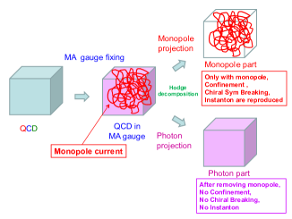
Figure 1: An illustration of the relevant role of monopoles to nonperturbative QCD. In the maximally Abelian gauge, QCD becomes Abelian-like due to the large off-diagonal gluon mass of about 1GeV [9], and there appears a global network of the monopole current [7, 8]. By the Hodge decomposition, the QCD system can be divided into the monopole part and the photon part. The monopole part has confinement [8], chiral symmetry breaking [3] and instantons [10], while the photon part does not have all of them.

However, as a possibility, removing the monopoles may be “too fatal” for most nonperturbative properties. If this is the case, nonperturbative QCD phenomena are simultaneously lost by their cut.

In fact, if only the relevant ingredient of chiral symmetry breaking is carefully removed, how will be confinement? To get the answer, we perform a direct investigation between confinement and chiral symmetry breaking, using the Dirac-mode expansion and projection [11].

2 Gauge-invariant formalism of Dirac-mode expansion and projection

In this paper, we develop a manifestly gauge-covariant expansion/projection of QCD operators such as the Wilson loop and the Polyakov loop, using the eigen-mode of the QCD Dirac operator ${\ooalign{\hfil/\hfil\crcr$D$}}=\gamma^{\mu}D^{\mu}$, and investigate the relation between confinement and chiral symmetry breaking [11].

2.1 Eigen-mode of Dirac operator in lattice QCD

In lattice QCD with spacing $a$, the Dirac operator ${\ooalign{\hfil/\hfil\crcr$D$}}=\gamma_{\mu}D_{\mu}$ is expressed with $U_{\mu}(x)$ as

$${\ooalign{\hfil/\hfil\crcr$D$}}_{x,y}\equiv\frac{1}{2a}\sum_{\mu=1}^{4}\gamma_{\mu}\left[U_{\mu}(x)\delta_{x+\hat{\mu},y}-U_{-\mu}(x)\delta_{x-\hat{\mu},y}\right],$$ (3)

with $U_{-\mu}(x)\equiv U^{\dagger}_{\mu}(x-\hat{\mu})$. Adopting hermitian $\gamma$-matrices $\gamma_{\mu}^{\dagger}=\gamma_{\mu}$, / $D$ is anti-hermitian and satisfies ${\ooalign{\hfil/\hfil\crcr$D$}}_{y,x}^{\dagger}=-{\ooalign{\hfil/\hfil\crcr$D$}}_{x,y}$. The normalized eigen-state $|n\rangle$ of the Dirac operator / $D$ is introduced as

$${\ooalign{\hfil/\hfil\crcr$D$}}|n\rangle=i\lambda_{n}|n\rangle$$ (6)

with $\lambda_{n}\in{\bf R}$. Because of $\{\gamma_{5},{\ooalign{\hfil/\hfil\crcr$D$}}\}=0$, the state $\gamma_{5}|n\rangle$ is also an eigen-state of / $D$ with the eigenvalue $-i\lambda_{n}$. The Dirac eigenfunction $\psi_{n}(x)\equiv\langle x|n\rangle$ obeys ${\ooalign{\hfil/\hfil\crcr$D$}}\psi_{n}(x)=i\lambda_{n}\psi_{n}(x)$, and its explicit form of the eigenvalue equation in lattice QCD is

$$\frac{1}{2a}\sum_{\mu=1}^{4}\gamma_{\mu}[U_{\mu}(x)\psi_{n}(x+\hat{\mu})-U_{-\mu}(x)\psi_{n}(x-\hat{\mu})]=i\lambda_{n}\psi_{n}(x).$$ (7)

The Dirac eigenfunction $\psi_{n}(x)$ can be numerically obtained in lattice QCD, besides a phase factor.

According to $U_{\mu}(x)\rightarrow V(x)U_{\mu}(x)V^{\dagger}(x+\hat{\mu})$, the gauge transformation of $\psi_{n}(x)$ is found to be

$$\psi_{n}(x)\rightarrow V(x)\psi_{n}(x),$$ (8)

which is the same as that of the quark field. To be strict, for the Dirac eigenfunction, there can appear an irrelevant $n$-dependent global phase factor as $e^{i\varphi_{n}[V]}$, according to the arbitrariness of the definition of $\psi_{n}(x)$.

From the Banks-Casher relation [12], the quark condensate $\langle\bar{q}q\rangle$, the order parameter of chiral symmetry breaking, is given by the zero-eigenvalue density $\rho(0)$ of the Dirac operator / $D$ :

$$\langle\bar{q}q\rangle=-\lim_{m\to 0}\lim_{V\to\infty}\pi\rho(0),$$ (9)

where the spectral density $\rho(\lambda)$ is given by $\rho(\lambda)\equiv\frac{1}{V}\sum_{n}\langle\delta(\lambda-\lambda_{n})\rangle$ with space-time volume $V$. Thus, the low-lying Dirac modes can be regarded as the essential modes responsible to spontaneous chiral-symmetry breaking in QCD.

2.2 Operator formalism in lattice QCD

The recent analysis of QCD with the Fourier expansion of the gluon field quantitatively reveals that quark confinement originates from low-momentum gluons below about 1GeV in both Landau and Coulomb gauges [13]. This method seems powerful but accompanies some gauge dependence. To keep the gauge symmetry manifestly, we take the “operator formalism” in lattice QCD [11].

We define the link-variable operator $\hat{U}_{\mu}$ by the matrix element of

$$\langle x|\hat{U}_{\mu}|y\rangle=U_{\mu}(x)\delta_{x+\hat{\mu},y}.$$ (10)

The Wilson-loop operator $\hat{W}$ is defined as the product of $\hat{U}_{\mu}$ along a rectangular loop,

$$\hat{W}\equiv\prod_{k=1}^{N}\hat{U}_{\mu_{k}}=\hat{U}_{\mu_{1}}\hat{U}_{\mu_{2}}\cdots\hat{U}_{\mu_{N}}.$$ (11)

For arbitrary loops, one finds $\sum_{k=1}^{N}\hat{\mu}_{k}=0$. We note that the functional trace of the Wilson-loop operator $\hat{W}$ is proportional to the ordinary vacuum expectation value $\langle W\rangle$ of the Wilson loop:

$${\rm Tr}\ \hat{W} = {\rm tr}\sum_{x}\langle x|\hat{W}|x\rangle={\rm tr}\sum_{x}\langle x|\hat{U}_{\mu_{1}}\hat{U}_{\mu_{2}}\cdots\hat{U}_{\mu_{N}}|x\rangle$$ (12)

$$= {\rm tr}\sum_{x_{1},x_{2},\cdots,x_{N}}\langle x_{1}|\hat{U}_{\mu_{1}}|x_{2}\rangle\langle x_{2}|\hat{U}_{\mu_{2}}|x_{3}\rangle\langle x_{3}|\hat{U}_{\mu_{3}}|x_{4}\rangle\cdots\langle x_{N}|\hat{U}_{\mu_{N}}|x_{1}\rangle$$

$$= {\rm tr}\sum_{x}\langle x|\hat{U}_{\mu_{1}}|x+\hat{\mu}_{1}\rangle\langle x+\hat{\mu}_{1}|\hat{U}_{\mu_{2}}|x+\sum_{k=1}^{2}\hat{\mu}_{k}\rangle\cdots\langle x+\sum_{k=1}^{N-1}\hat{\mu}_{k}|\hat{U}_{\mu_{N}}|x\rangle$$

$$= \sum_{x}{\rm tr}\{U_{\mu_{1}}(x)U_{\mu_{2}}(x+\hat{\mu}_{1})U_{\mu_{3}}(x+\sum_{k=1}^{2}\hat{\mu}_{k})\cdots U_{\mu_{N}}(x+\sum_{k=1}^{N-1}\hat{\mu}_{k})\}=\langle W\rangle\cdot{\rm Tr}\ 1.$$

Here, “Tr” denotes the functional trace, and “tr” the trace over SU(3) color index.

The Dirac-mode matrix element of the link-variable operator $\hat{U}_{\mu}$ can be expressed with $\psi_{n}(x)$:

$$\langle m|\hat{U}|n\rangle=\sum_{x}\langle m|x\rangle\langle x|\hat{U}_{\mu}|x+\hat{\mu}\rangle\langle x+\hat{\mu}|n\rangle=\sum_{x}\psi_{m}^{\dagger}(x)U_{\mu}(x)\psi_{n}(x+\hat{\mu}).$$ (13)

Although the total number of the matrix element is very huge, the matrix element is calculable and gauge invariant, apart from an irrelevant phase factor. Using the gauge transformation (8), we find the gauge transformation of the matrix element as [11]

$$\langle m|\hat{U}_{\mu}|n\rangle = \sum_{x}\psi^{\dagger}_{m}(x)U_{\mu}(x)\psi_{n}(x+\hat{\mu})$$ (14)

$$\rightarrow \sum_{x}\psi^{\dagger}_{m}(x)V^{\dagger}(x)\cdot V(x)U_{\mu}(x)V^{\dagger}(x+\hat{\mu})\cdot V(x+\hat{\mu})\psi_{n}(x+\hat{\mu})$$

$$= \sum_{x}\psi_{m}^{\dagger}(x)U_{\mu}(x)\psi_{n}(x+\hat{\mu})=\langle m|\hat{U}_{\mu}|n\rangle.$$

To be strict, there appears an $n$-dependent global phase factor, corresponding to the arbitrariness of the phase in the basis $|n\rangle$. However, this phase factor cancels as $e^{-i\varphi_{n}}e^{i\varphi_{n}}=1$ between $|n\rangle$ and $\langle n|$, and does not appear for QCD physical quantities including the Wilson loop.

2.3 Dirac-mode expansion and projection

From the completeness of the Dirac-mode basis, $\sum_{n}|n\rangle\langle n|=1$, arbitrary operator $\hat{O}$ can be expanded in terms of the Dirac-mode basis $|n\rangle$ as

$$\hat{O}=\sum_{n}\sum_{m}|n\rangle\langle n|\hat{O}|m\rangle\langle m|,$$ (15)

which is the theoretical basis of the Dirac-mode expansion [11]. Note here that this procedure is just the insertion of unity, and is of course mathematically correct.

Based on this relation, the Dirac-mode expansion and projection can be defined. We define the projection operator $\hat{P}$ which restricts the Dirac-mode space,

$$\hat{P}\equiv\sum_{n\in A}|n\rangle\langle n|,$$ (16)

where $A$ denotes arbitrary set of Dirac modes. In $\hat{P}$, the arbitrary phase cancels between $|n\rangle$ and $\langle n|$. One finds $\hat{P}^{2}=\hat{P}$ and $\hat{P}^{\dagger}=\hat{P}$. The typical projections are IR-cut and UV-cut of the Dirac modes:

$$\hat{P}_{\rm\ IR}\equiv\sum_{|\lambda_{n}|\geq\Lambda_{\rm IR}}|n\rangle\langle n|,\qquad\hat{P}_{\rm\ UV}\equiv\sum_{|\lambda_{n}|\leq\Lambda_{\rm UV}}|n\rangle\langle n|.$$ (17)

Using the projection operator $\hat{P}$, we define the Dirac-mode projected link-variable operator,

$$\hat{U}^{P}_{\mu}\equiv\hat{P}\hat{U}_{\mu}\hat{P}=\sum_{m\in A}\sum_{n\in A}|m\rangle\langle m|\hat{U}_{\mu}|n\rangle\langle n|.$$ (18)

During this projection, there appears some nonlocality in general, but it would not be important for the argument of large-distance properties such as confinement. From the Wilson-loop operator $\hat{W}\equiv\prod_{k=1}^{N}\hat{U}_{\mu_{k}}$, we define the Dirac-mode projected Wilson-loop operator $\hat{W}^{P}\equiv\prod_{k=1}^{N}\hat{U}^{P}_{\mu_{k}}$, and rewrite its functional trace in terms of the Dirac basis as [11]

$${\rm Tr}\ \hat{W}^{P} = {\rm Tr}\ \prod_{k=1}^{N}\hat{U}^{P}_{\mu_{k}}={\rm Tr}\ \hat{U}^{P}_{\mu_{1}}\hat{U}^{P}_{\mu_{2}}\cdots\hat{U}^{P}_{\mu_{N}}={\rm Tr}\ \hat{P}\hat{U}_{\mu_{1}}\hat{P}\hat{U}_{\mu_{2}}\hat{P}\cdots\hat{P}\hat{U}_{\mu_{N}}\hat{P}$$ (19)

$$= {\rm tr}\sum_{n_{1},n_{2},\cdots,n_{N}\in A}\langle n_{1}|\hat{U}_{\mu_{1}}|n_{2}\rangle\langle n_{2}|\hat{U}_{\mu_{2}}|n_{3}\rangle\cdots\langle n_{N}|\hat{U}_{\mu_{N}}|n_{1}\rangle,$$

which is manifestly gauge invariant. Here, the arbitrary phase factor cancels between $|n_{k}\rangle$ and $\langle n_{k}|$. Its gauge invariance is also numerically checked in the lattice QCD Monte Carlo calculation.

From ${\rm Tr}\ \hat{W}^{P}(R,T)$ on the $R\times T$ rectangular loop, we define Dirac-mode projected potential,

$$V^{P}(R)\equiv-\lim_{T\to\infty}\frac{1}{T}{\rm ln}\{{\rm Tr}\ \hat{W}^{P}(R,T)\}.$$ (20)

On a periodic lattice of $V=L^{3}\times N_{t}$, we define the Dirac-mode projected Polyakov loop [11]:

$$\langle L_{P}^{\rm proj.}\rangle\equiv\frac{1}{3V}{\rm Tr}\ \prod_{i=1}^{N_{t}}\hat{U}_{4}^{P}=\frac{1}{3V}{\rm Tr}\ (\hat{U}_{4}^{P})^{N_{t}}=\frac{1}{3V}{\rm tr}\sum_{n_{1},..,n_{N_{t}}\in A}\langle n_{1}|\hat{U}_{4}|n_{2}\rangle\langle n_{2}|\hat{U}_{4}|n_{3}\rangle\cdots\langle n_{N_{t}}|\hat{U}_{4}|n_{1}\rangle,~{}~{}~{}~{}~{}~{}~{}$$ (21)

which is also manifestly gauge-invariant.

3 Analysis of confinement in terms of Dirac modes in QCD

In this paper, we mainly consider the removal of low-lying Dirac modes, i.e., the IR-cut case. Using the Dirac-mode expansion and projection method, we calculate the IR-Dirac-mode-cut Wilson loop ${\rm Tr}~{}W^{P}(R,T)$, the IR-cut inter-quark potential $V^{P}(R)$, and the IR-Dirac-mode-cut Polyakov loop $\langle L_{P}\rangle_{\rm IR}$ in a gauge-invariant manner [11]. Here, we can directly investigate the relation between chiral symmetry breaking and confinement as the area-law behavior of the Wilson loop, since the low-lying Dirac modes are responsible to chiral symmetry breaking.

As a technical difficulty, we have to deal with huge dimensional matrices and their products. Actually, the total matrix dimension of $\langle m|\hat{U}_{\mu}|n\rangle$ is (Dirac-mode number)². On the $L^{4}$ lattice, the Dirac-mode number is $L^{4}\times N_{c}\times$ 4, which can be reduced to be $L^{4}\times N_{c}$, using the Kogut-Susskind technique [5]. Even for the projected operator, where the Dirac-mode space is restricted, the matrix is generally still huge. At present, we use a small-size lattice in the actual lattice QCD calculation.

We use SU(3) lattice QCD with the standard plaquette action at $\beta=5.6$ (i.e., $a\simeq 0.25{\rm fm}$) on $6^{4}$ at the quenched level. The periodic boundary condition is imposed for the gauge field. We show in Fig.2(a) the spectral density $\rho(\lambda)$ of the QCD Dirac operator / $D$ . The chiral property of / $D$ leads to $\rho(-\lambda)=\rho(\lambda)$. Figure 2(b) is the IR-cut Dirac spectral density $\rho_{\rm IR}(\lambda)\equiv\rho(\lambda)\theta(|\lambda|-\Lambda_{\rm IR})$ with the IR-cutoff $\Lambda_{\rm IR}=0.5a^{-1}\simeq 0.4{\rm GeV}$. By removing the low-lying Dirac modes, the chiral condensate is largely reduced as $\langle\bar{q}q\rangle_{\Lambda_{\rm IR}}/\langle\bar{q}q\rangle\simeq 0.02$ around the physical region of $m_{q}\simeq 5{\rm MeV}$.

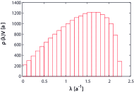
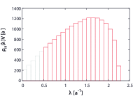
Figure 2: (a) The Dirac spectral density $\rho(\lambda)$ in lattice QCD at $\beta$=5.6 and $6^{4}$. The volume $V$ is multiplied. (b) The IR-cut Dirac spectral density $\rho_{\rm IR}(\lambda)\equiv\rho(\lambda)\theta(|\lambda|-\Lambda_{\rm IR})$ with the IR-cutoff $\Lambda_{\rm IR}=0.5a^{-1}\simeq 0.4{\rm GeV}$.

Figure 3 shows the IR-Dirac-mode-cut Wilson loop $\langle W^{P}(R,T)\rangle\equiv{\rm Tr}\hat{W}^{P}(R,T)$, the IR-cut inter-quark potential $V^{P}(R)$, and the IR-Dirac-mode-cut Polyakov loop $\langle L_{P}\rangle_{\rm IR}$, after the removal of the low-lying Dirac modes. These Dirac-mode projected quantities are obtained in lattice QCD with the IR-cut of $\rho_{\rm IR}(\lambda)\equiv\rho(\lambda)\theta(|\lambda|-\Lambda_{\rm IR})$ with the IR-cutoff $\Lambda_{\rm IR}=0.5a^{-1}\simeq 0.4{\rm GeV}$.

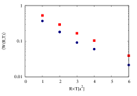
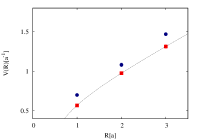
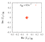
Figure 3: The attice QCD results after the removal of low-lying Dirac modes [11], which gives $\rho_{\rm IR}(\lambda)\equiv\rho(\lambda)\theta(|\lambda|-\Lambda_{\rm IR})$ with the IR-cutoff $\Lambda_{\rm IR}=0.5a^{-1}\simeq 0.4{\rm GeV}$. (a) The IR-cut Wilson loop ${\rm Tr}~{}W^{P}(R,T)$ (circle) after removing the IR Dirac modes, plotted against $R\times T$. The slope parameter $\sigma^{P}$ is almost the same as that of the original Wilson loop (square). (b) The IR-cut inter-quark potential (circle), which is almost unchanged from the original one (square), apart from an irrelevant constant. (c) The scatter plot of the IR-Dirac-mode-cut Polyakov loop $\langle L_{P}\rangle_{\rm IR}$: its zero-value indicates $Z_{3}$-unbroken confinement phase.

Remarkably, even after removing the coupling to the low-lying Dirac modes, which are responsible to chiral symmetry breaking, the IR-Dirac-mode-cut Wilson loop is found to obey the area law as $\langle W^{P}(R,T)\rangle\propto e^{-\sigma^{P}RT}$, and the slope parameter $\sigma^{P}$ corresponding to the string tension or the confinement force is almost unchanged as $\sigma^{P}\simeq\sigma$. Accordingly, as shown in Fig.3(b), the IR-cut inter-quark potential $V^{P}(R)$ is almost unchanged from the original one, apart from an irrelevant constant. Also from Fig.3(c), we find that the IR-Dirac-mode-cut Polyakov loop is almost zero, i.e., $\langle L_{P}\rangle_{\rm IR}\simeq 0$, which indicates $Z_{3}$-unbroken confinement phase. In fact, quark confinement is kept in the absence of the low-lying Dirac modes or the essence of chiral symmetry breaking [11]. This result seems consistent with Gattringer’s formula [4] and Lang-Schrock’s result [14].

We also investigate the UV-cut of Dirac modes in lattice QCD, and find that the confining force is almost unchanged by the UV-cut [11], which seems consistent with the lattice result of Synatschke-Wipf-Langfeld [15]. Furthermore, we examine “intermediate-cut” of Dirac modes, and obtain almost the same confining force [11]. Then, we conjecture that the “seed” of confinement is distributed not only in low-lying Dirac modes but also in a wider region of the Dirac-mode space.

Our lattice QCD results suggest some independence between chiral symmetry breaking and color confinement, which may lead to richer phase structure in QCD. For example, the phase transition point can be different between deconfinement and chiral restoration in the presence of strong electro-magnetic fields, because of their nontrivial effect on chiral symmetry [16].

References

• [1] Y. Nambu and G. Jona-Lasinio, Phys. Rev. 122 (1961) 345; ibid. 124 (1961) 246.
• [2] H. Suganuma, S. Sasaki and H. Toki, Nucl. Phys. B435 (1995) 207; Prog. Theor. Phys. 94 (1995) 373.
• [3] O. Miyamura, Phys. Lett. B353 (1995) 91; R.M. Woloshyn, Phys. Rev. D51 (1995) 6411.
• [4] C. Gattringer, Phys. Rev. Lett. 97 (2006) 032003; F. Bruckmann et al., Phys. Lett. B647 (2007) 56.
• [5] H.-J. Rothe, Lattice Gauge Theories, 4th edition, World Scientific, 2012.
• [6] Y. Nambu, Phys. Rev. D10 (1974) 4262; G. ’t Hooft, Nucl. Phys. B190 (1981) 455.
• [7] A.S. Kronfeld, G. Schierholz and U.-J. Wiese, Nucl. Phys. B293 (1987) 461.
• [8] J.D. Stack, S.D. Neiman and R.J. Wensley, Phys. Rev. D50 (1994) 3399 [hep-lat/9404014].
• [9] K. Amemiya and H. Suganuma, Phys. Rev. D60 (1999) 114509 [hep-lat/9811035];
S. Gongyo, T. Iritani and H. Suganuma, Phys. Rev. D86 (2012) [arXiv:1207.4377 [hep-lat]].
• [10] H. Suganuma, A. Tanaka, S. Sasaki and O. Miyamura, Nucl. Phys. Proc. Suppl. 47 (1996) 302.
• [11] S. Gongyo, T. Iritani and H. Suganuma, Phys. Rev. D86 (2012) 034510 [arXiv:1202.4130 [hep-lat]];
H. Suganuma, S. Gongyo, T. Iritani and A. Yamamoto, PoS (QCD-TNT-II), 044 (2011).
• [12] T. Banks and A. Casher, Nucl. Phys. B169 (1980) 103.
• [13] A. Yamamoto and H. Suganuma, Phys. Rev. Lett. 101 (2008) 241601; Phys. Rev. D79 (2009) 054504.
• [14] C.B. Lang and M. Schrock, Phys. Rev. D84 (2011) 087704 [arXiv:1107.5195 [hep-lat]];
L.Ya Glozman, C.B. Lang and M. Schrock, Phys. Rev. D86 (2012) 014507.
• [15] F. Synatschke, A. Wipf and K. Langfeld, Phys. Rev. D77 (2008) 114018 [arXiv:0803.0271 [hep-lat]].
• [16] H. Suganuma and T. Tatsumi, Ann. Phys. 208 (1991) 470; Prog. Theor. Phys. 90 (1993) 379.