NLO parton shower for LHC physics -
hard processes and beyond

Abstract:

The new methodology of adding QCD NLO corrections in the initial state Monte Carlo parton shower (hard process part) is presented using process of the heavy boson production at the LHC as an example. Despite the simplified model of the process, presented numerical results prove that the basic concept of the new methodology works correctly in the numerical environment of the Monte Carlo parton shower event generator. The presented method is an alternative to the well established methods, MC@NLO and POWHEG. Refinements of the new method with better computer CPU time efficiency are also discussed.

1 Introduction

The Large Hadron Collider (LHC) at CERN provides rich harvest of experimental data. The proper understanding and interpretation of these data, possibly leading to discovery of new phenomena, requires perfect mastering of the “trivial” effects due to the multiple emissions of soft and collinear gluons and quarks. Perturbative Quantum Chromodynamics (pQCD) [1, 2, 3], supplemented with clever modelling of the low energy nonperturbative effects, is an indispensable tool for disentangling the Standard Model physics component in the data. This work presents part of the global effort of improving quality of the pQCD calculations for LHC experiments.

Most of the results presented here are described in refs. [4] and [5]. Although this work elaborates on the improved method of the pQCD calculation combining NLO-corrected hard process and LO parton shower Monte Carlo (MC), it should be regarded as the first step towards NNLO-corrected hard process combined with the NLO parton shower MC [6].

2 Basic LO parton shower MC

The multigluon distribution of the single initial state ladder, which is a building block of our parton shower MC, is represented by the integrand of the “exclusive/unintegrated PDF”, which in the LO approximation is the following:

$$\begin{split}&D(t,x)=\int dx_{0}\;dZ\;\delta_{x=x_{0}Z}\;d_{0}(\hat{t}_{0},x_{0})\;G(t,\hat{t}_{0}-\ln x_{0}|Z),\\ &G(t,t_{0}|Z)=e^{-S_{F}}\sum_{n=0}^{\infty}\bigg{(}\prod_{i=1}^{n}\int d^{3}{\cal E}(\bar{k}_{i})\;\theta_{\xi_{i}>\xi_{i-1}}\frac{2C_{F}\alpha_{s}}{\pi^{2}}\bar{P}(z_{i})\bigg{)}\\ &\qquad\qquad\quad\times\theta_{t>\xi_{n}}\delta_{Z=\prod_{j=1}^{n}z_{j}},\end{split}$$ (1)

where evolution kernel is $\bar{P}(z)=\frac{1}{2}(1+z^{2})$, evolution time is $\hat{t}_{0}=\ln(q_{0}/\Lambda)$ and the “eikonal” phase space integration element is $d^{3}{\cal E}(k)=\frac{d^{3}k}{2k^{0}}\;\frac{1}{{\bf{k}}^{2}}=\pi\frac{d\phi}{2\pi}\frac{dk^{+}}{k^{+}}d\xi$ and $k^{\pm}=k^{0}\pm k^{3}$. We use rapidities $\xi_{i}=\frac{1}{2}\ln\frac{k^{-}_{i}}{k^{+}_{i}}\big{|}_{\rm Rh}$ in the hadron beam rest frame (Rh), and $\eta_{i}=\frac{1}{2}\ln\frac{k^{+}_{i}}{k^{-}_{i}}\big{|}_{\rm RFHP}$ defined in hard process rest frame (RFHP). They are related by $\xi_{i}=\ln\frac{\sqrt{s}}{m_{h}}-\eta_{i}$. Rapidity ordering is now $t=\xi_{\max}>\xi_{n}>\dots>\xi_{i}>\xi_{i-1}>\dots>\xi_{0}=t_{0}$, where $t_{0}=\xi_{0}=\ln(q_{0}/m_{h})-\ln x_{0}$. The direction of the $z$ axis in the RFHP is pointing out towards the hadron momentum. A lightcone variable of the emitted gluon is defined as $\alpha_{i}=\frac{2k_{i}^{+}}{\sqrt{s}}$ and of the emitter parton (quark) as $x_{i}=x_{0}-\sum_{j=0}^{i}\;\alpha_{j}$ (after $i$ emissions). We also use fractions $z_{i}=x_{i}/x_{i-1}$. The Sudakov formfactor $S_{F}$ comes from the “unitarity” condition $\int_{0}^{1}dZ\;G(t,t_{0}|Z)=1,$ which is also instrumental in the Markovian MC implementation used to obtain $D(t,x)$ at any value of $t>t_{0}$.

The initial distribution $d_{0}(q_{0},x_{0})$ related to experiment, to previous steps in the MC ladder, or to PDF in the standard $\overline{MS}$ system is not essential for the following discussion, we only note that the unitarity condition provides baryon number conservation sum rule $\int_{0}^{1}dx\;D(t,x)=\int_{0}^{1}dx_{0}\;d_{0}(t_{0},x_{0})$.

For testing our new method of correcting hard process to the NLO level we use the following simplified MC parton shower, implementing the DY process with two ladders and the hard process:

$$\begin{split}&\sigma_{0}=\int dx_{0F}dx_{0B}\;\;d_{0}(\hat{t}_{0},x_{0F})d_{0}(\hat{t}_{0},x_{0B})\sum_{n_{1}=0}^{\infty}\;\sum_{n_{2}=0}^{\infty}\int dx_{F}\;dx_{B}\;\\ &~{}~{}~{}~{}~{}~{}~{}~{}~{}\times e^{-S_{{}_{F}}}\int_{\Xi<\eta_{n_{1}}}\bigg{(}\prod_{i=1}^{n_{1}}d^{3}{\cal E}(\bar{k}_{i})\theta_{\eta_{i}<\eta_{i-1}}\frac{2C_{F}\alpha_{s}}{\pi^{2}}\bar{P}(z_{Fi})\bigg{)}\delta_{x_{F}=x_{0F}\prod_{i=1}^{n_{1}}z_{Fi}}\\ &~{}~{}~{}~{}~{}~{}~{}~{}~{}\times e^{-S_{{}_{B}}}\int_{\Xi>\eta_{n_{2}}}\bigg{(}\prod_{j=1}^{n_{2}}d^{3}{\cal E}(\bar{k}_{j})\theta_{\eta_{j}>\eta_{j-1}}\frac{2C_{F}\alpha_{s}}{\pi^{2}}\bar{P}(z_{Bj})\bigg{)}\delta_{x_{B}=x_{0B}\prod_{j=1}^{n_{2}}z_{Bj}}\\ &~{}~{}~{}~{}~{}~{}~{}~{}~{}\times d\tau_{2}(P-\sum_{j=1}^{n_{1}+n_{2}}k_{j};q_{1},q_{2})\;\frac{d\sigma_{B}}{d\Omega}(sx_{F}x_{B},\hat{\theta})\;W^{NLO}_{MC}.\end{split}$$ (2)

In the LO approximation $W^{NLO}_{MC}=1$. Rapidity $\xi$ is translated into $\eta$ – the center of mass system rapidity, in the forward part (F) of the phase space as $\xi_{i}=\ln\frac{\sqrt{s}}{m_{h}}-\eta_{i}$, $\eta_{0F}>\eta_{i}>\Xi$, and in the backward (B) part as $\xi_{i}=-\ln\frac{\sqrt{s}}{m_{h}}+\eta_{i}$, $\Xi>\eta_{i}>\eta_{0B}$. The rapidity boundary between the two hemispheres $\Xi=0$ is used, until a more sophisticated version related to rapidity of the produced $W/Z$ is introduced.

Analytical integration of eq. (2) results in the standard factorization formula ($W^{NLO}_{MC}=1$)

$$\sigma_{0}=\int_{0}^{1}dx_{F}\;dx_{B}\;D_{F}(t,x_{F})\;D_{B}(t,x_{B})\;\sigma_{B}(sx_{F}x_{B}).$$ (3)

The distributions $D_{F}(t,x_{F})=(d_{0}\otimes G_{F})(t,x_{F})$ and $D_{B}(t,x_{B})=(d_{0}\otimes G_{B})(t,x_{B})$ are obtained from separate Markovian LO Monte Carlo runs. The above LO formula is exact, and can be tested with an arbitrary numerical precision.

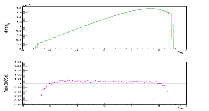
Figure 1: The upper plot shows the LO distribution of $\eta_{W}^{*}=\frac{1}{2}\ln(x_{F}/x_{B})$ from the CMC LO parton shower (purple) and from the strictly collinear formula (green). The lower plot shows the ratio of the two.

Figure 1 represents a “calibration benchmark” for the overall normalization at the LO level. We show there the properly normalized distribution of the variable $\eta_{W}^{*}=\frac{1}{2}\ln(x_{F}/x_{B})$, which in the collinear limit approximates the rapidity of $W$ boson. The distribution in the upper plot of Fig. 1, representing eq. (3), is obtained using the general purpose MC program FOAM [7]. The collinear PDF $D(t,x)$ there has been obtained from a separate high statistics run ($10^{10}$ events) of a Markovian MC (MMC), creating $D(t,x)$ in a form of the 2-dimensional look-up table. The other distribution in the upper plot of Fig. 1 represents eq. (2) in LO approximation. It comes from the full scale MC generation (with four-momenta conservation). The MC run with $10^{8}$ events was used. The constrained MC (CMC) technique of ref. [10] is used here because of the narrow Breit-Wigner peak due to a heavy boson propagator. Two CMC modules and FOAM are combined into one MC generating gluon emissions and the $W$ boson production. FOAM is taking care of the generation of the variables $x_{F},x_{B},x_{F0},x_{B0}$ and the sharp Breit-Wigner peak in $\hat{s}=sx_{F}x_{B}$, then two CMC modules are initialized and generate the gluon four-momenta $\bar{k}^{\mu}_{j}$. They are mapped into $k^{\mu}_{j}$, following the prescription defined in ref. [4], such that the overall energy-momentum conservation is achieved. Figure 1 demonstrates a very good numerical agreement between $d\sigma/d\eta_{W}^{*}$ from our full scale LO parton shower MC of eq. (2) and the simple formula of eq. (3), to within 0.5%, as seen from the ratio of the two results in the lower part of the figure.

3 Introducing NLO corrections to hard process

The NLO corrections to hard process are imposed on top of the LO distributions of eq. (2) using a single “monolithic” weight $W^{NLO}_{MC}$ defined exactly as in ref. [4]:

$$\begin{split}&W^{NLO}_{MC}=1+\Delta_{S+V}+\sum_{j\in F}\frac{{\tilde{\beta}}_{1}(q_{1},q_{2},\bar{k}_{j})}{\bar{P}(z_{Fj})\;d\sigma_{B}(\hat{s},\hat{\theta})/d\Omega}+\sum_{j\in B}\frac{{\tilde{\beta}}_{1}(q_{1},q_{2},\bar{k}_{j})}{\bar{P}(z_{Bj})\;d\sigma_{B}(\hat{s},\hat{\theta})/d\Omega},\end{split}$$ (4)

the NLO soft+virtual correction is $\Delta_{V+S}=\frac{C_{F}\alpha_{s}}{\pi}\;\left(\frac{2}{3}\pi^{2}-\frac{5}{4}\right)$, and the real correction reads:

$$\begin{split}&{\tilde{\beta}}_{1}(q_{1},q_{2},k)=\Big{[}\frac{(1-\beta)^{2}}{2}\frac{d\sigma_{B}}{d\Omega_{q}}(\hat{s},\theta_{F})+\frac{(1-\alpha)^{2}}{2}\frac{d\sigma_{B}}{d\Omega_{q}}(\hat{s},\theta_{B})\Big{]}\\ &~{}~{}~{}~{}~{}~{}~{}~{}~{}~{}~{}~{}~{}~{}~{}~{}~{}~{}~{}~{}-\theta_{\alpha>\beta}\frac{1+(1-\alpha-\beta)^{2}}{2}\frac{d\sigma_{B}}{d\Omega_{q}}(\hat{s},\hat{\theta})-\theta_{\alpha<\beta}\frac{1+(1-\alpha-\beta)^{2}}{2}\frac{d\sigma_{B}}{d\Omega_{q}}(\hat{s},\hat{\theta}).\end{split}$$ (5)

The above is the exact ME of the quark-antiquark annihilation into a heavy vector boson with additional single real gluon emission. The LO component, which is already included in the LO MC, is subtracted here. The variable $\hat{s}=sx_{F}x_{B}=(q_{1}+q_{2})^{2}$ is the effective mass squared of the heavy vector boson. The definition of angle $\hat{\theta}$ in the LO component is rather arbitrary. We define it in the rest frame of the heavy boson, where $\vec{q}_{1}+\vec{q}_{2}=0$, as an angle between the decay lepton momentum $\vec{q}_{1}$ and the difference of momenta of the incoming quark and antiquark $\hat{\theta}=\angle(\vec{q}_{1},\vec{p}_{0F}-\vec{p}_{0B})$. On the other hand the two angles in the NLO ME are defined quite unambiguously as $\hat{\theta}_{F}=\angle(\vec{q}_{1},-\vec{p}_{0B})$ and $\hat{\theta}_{B}=\angle(\vec{q}_{1},\vec{p}_{0F})$. In the above we only need directions of the $\vec{p}_{0F}$ and $\vec{p}_{0B}$ vectors, which are the same as the directions of the hadron beams. The lightcone variables $\alpha_{j}$ and $\beta_{j}$ of the emitted gluon are defined in the F and B parts of the phase space as follows:

$$\begin{split}&\alpha_{j}=1-z_{Fj},\quad\beta_{j}=\alpha_{j}\;e^{2(\eta_{j}-\Xi)},\quad~{}~{}{\rm for}~{}~{}~{}j\in F,\\ &\beta_{j}=1-z_{Bj},\quad\alpha_{j}=\beta_{j}\;e^{-2(\eta_{j}-\Xi)},\quad{\rm for}~{}~{}~{}j\in B.\end{split}$$

Again, the exact phase space integration of eq. (2) including $W^{NLO}_{MC}$ of eq. (4) is feasible, and the resulting compact expression for the total cross section is obtained [4]:

$$\begin{split}\sigma_{1}&=\int_{0}^{1}dx_{F}\;dx_{B}\;dz\;D_{F}(t,x_{F})\;D_{B}(t,x_{B})\;\sigma_{B}(szx_{F}x_{B})\big{\{}\delta_{z=1}(1+\Delta_{S+V})+C_{2r}(z)\big{\}},\end{split}$$ (6)

where $C_{2r}(z)=\frac{2C_{F}\alpha_{s}}{\pi}\;\left[-\frac{1}{2}(1-z)\right].$

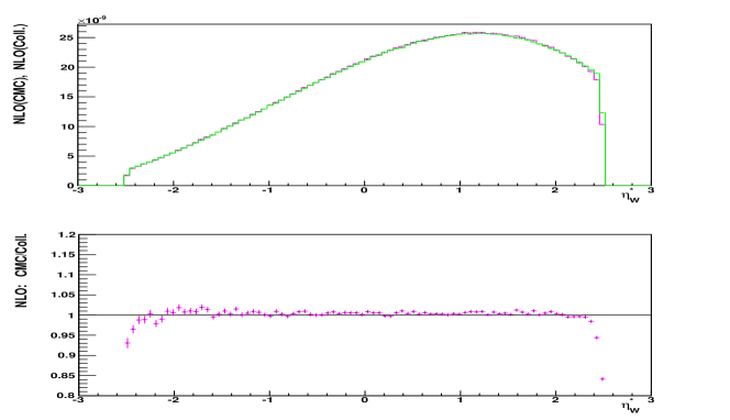
Figure 2: The upper plot shows $(-)$ NLO correction (alone) to the distribution of $\eta_{W}^{*}=\frac{1}{2}\ln(x_{F}/x_{B})$ from the parton shower (purple) and from the the strictly collinear formula (green). Their ratio is plotted below.

3.1 Numerical test of NLO correction

Figure 2 represents a principal proof of concept of our new methodology for implementing the NLO corrections to the hard process in the parton shower MC. The plotted NLO correction to the $\eta_{W}^{*}$ distribution comes from the parton shower MC with the NLO-corrected hard process according to eqs. (2) and (4). Additionally we also plot there result of a simple collinear formula of eq. (6), where two collinear PDFs are convoluted with the analytical coefficient function $C_{2r}(z)$ for the hard process. Both results coincide within the statistical error, see their ratio in the lower part of Fig. 2.

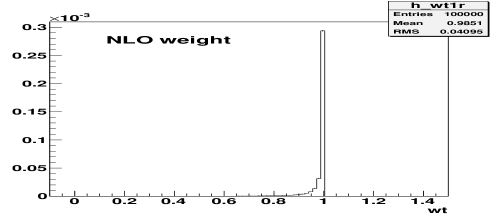
Figure 3: The distribution of the NLO weight $W^{NLO}_{MC}$ of eq. (4).

Technically, the inclusion of the NLO correction in our parton shower MC is rather straightforward, and is obtained by including $W^{NLO}_{MC}$ weight of eq. (4). MC is providing both LO and NLO-corrected results in a single run with weighted events. The NLO weight is strongly peaked near $W^{NLO}_{MC}=1$, positive, and without long-range tails. Its distribution is shown in Fig. 3.

In all numerical results we have set $\Delta_{V+S}=0$, as it is completely unimportant for the presented analysis. The initial distributions $d_{0}(q_{0},x_{0})$ are defined in ref. [5].

4 Simplification of the method and comparison with other methodologies

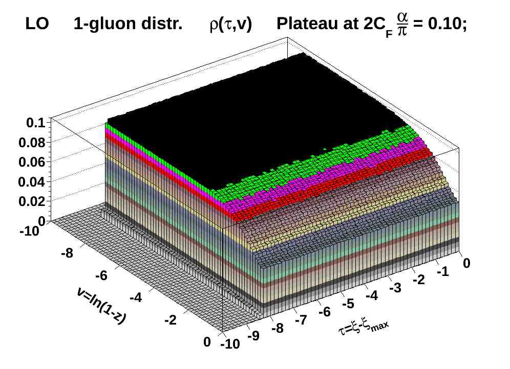
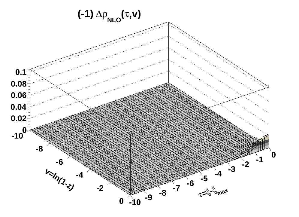
Figure 4: The inclusive distribution of gluons on the log Sudakov plane of rapidity $t=\xi$ and $v=\ln(1-z)$ (LHS). Contributions from all gluons weighted with the component weight $W^{NLO}_{j}$ (RHS).

Our new method for introducing NLO corrections in the hard process, proposed in ref. [4] and tested in ref. [5], is an alternative to the two well established MC@NLO [14] and POWHEG [15, 16] methodologies. With MC numerical implementation at hand, let us elaborate on the differences with the above two techniques in particular with the POWHEG technique. We shall also see that it is possible to make our method more efficient in terms of CPU time consumption. This improvement is not so critical in the present case of NLO corrected hard process, but may be quite useful in the case of correcting evolution kernels to the NLO in the ladder parts of the MC [6].

The most important differences with the POWHEG and MC@NLO techniques are:

• The summation over all emitted gluons, without deciding which gluon is the one involved in the NLO correction and which ones are merely “LO spectators” in the parton shower.

• The absence of $(1/(1-z))_{+}$ distributions in the real part of the NLO corrections (virtual+soft correction is kinematically independent).

To explain more clearly how $W^{NLO}_{MC}$ of eq. (4) is distributed over the multigluon phase space, we restrict now to single ladder (hemisphere) with a simplified weight:

$$\begin{split}&W^{NLO}_{MC}=1+\sum_{j\in F}W^{NLO}_{j},\qquad W^{NLO}_{j}=\frac{{\tilde{\beta}}_{1}(q_{1},q_{2},\bar{k}_{j})}{\bar{P}(z_{Fj})\;d\sigma_{B}(\hat{s},\hat{\theta})/d\Omega}.\end{split}$$ (7)

In order to find out the phase space regions specific for NLO corrections we consider inclusive distributions of gluons on the Sudakov logarithmic plane of rapidity $\xi$ and variable $v=\ln(1-z)$. In the left hand side (LHS) of Fig. 4 we show gluons inclusive distribution in the LO approximation. The flat plateau there represents IR/collinear singularity $2C_{F}\frac{\alpha_{S}}{\pi}d\xi\frac{dz}{1-z}$ with the drop by factor 1/2 towards $z=0$, due to $\frac{1+z^{2}}{2}$ factor in the LO kernel. In the right hand side (RHS) of Fig. 4 we show contributions from all gluons weighted with the component weight $-W^{NLO}_{j}$ of eq. (7). The NLO contribution is concentrated in the area near the hard process rapidity $t=\xi_{\max}$, which has to be true for the genuine NLO contribution. The completeness of the phase space near this important region ($z=0$, $\xi_{\max}$) is critical for the completeness of the NLO corrections. Both POWHEG and MC@NLO use standard LO MCs which feature an empty “dead zone” in this phase space corner.

Figure 4 suggests that the dominant contribution to $\sum_{j}W^{NLO}_{j}$ could be from the gluon with the maximum $\ln k_{j}^{T}\sim\xi_{j}+\ln(1-z_{j})$, which is closest to the hard process phase space corner. In the MC we may easily relabel generated gluons using new index $K$ such that they are ordered in the variable $\kappa_{K}=\xi_{K}+\ln(1-z_{K}),\;\kappa_{K+1}<\kappa_{K}$ with $K=1$ being the hardest one.

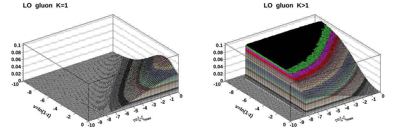
Figure 5: The inclusive LO distribution of Fig. 4 split into the hardest gluon (left) and the rest (right).

Figure 5 demonstrates a split of the LO inclusive distribution of Fig. 4 into the $K=1$ component and the rest $K>1$. The important point is that the $K=1$ component reproduces the original complete distribution over the whole region where the NLO correction is non-negligible! This is exactly the observation on which POWHEG technique is built. According to the POWHEG authors, taking the $K=1$ component is sufficient to reproduce the complete NLO correction (modulo NNLO).

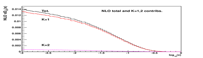
Figure 6: The original NLO correction from $\sum_{j}W^{NLO}_{j}$ and its two hardest gluon components, from $W^{NLO}_{K=1}$ and $W^{NLO}_{K=2}$, as a function of $x=\prod_{j}z_{j}$.

The above statement is checked numerically in Fig. 6, where we compare the NLO correction to the $x=\prod_{j}z_{j}$ distribution from the complete sum $\sum_{j}W^{NLO}_{j}$ and from $W^{NLO}_{K=1}$. As we see the $K=1$ component saturates the complete sum very well, with the $K=2$ component being negligible in the first approximation.

We can therefore speed up the calculation by means of taking only the $K=1$ contribution. The price will be that the formula of eq. (6) will not be exact any more. Our method differs, however, from the POWHEG scheme, where the $K=1$ gluon is generated separately in the first step, and other gluons are generated (by the LO parton shower MC) in the next step. That is easy for LO MC with $k^{T}$-ordering, while in case of the LO MC with angular-ordering POWHEG requires additional effort of generating the so called vetoed and truncated showers. In our method, there is no need for such vetoed/truncated showers in case of angular ordering.

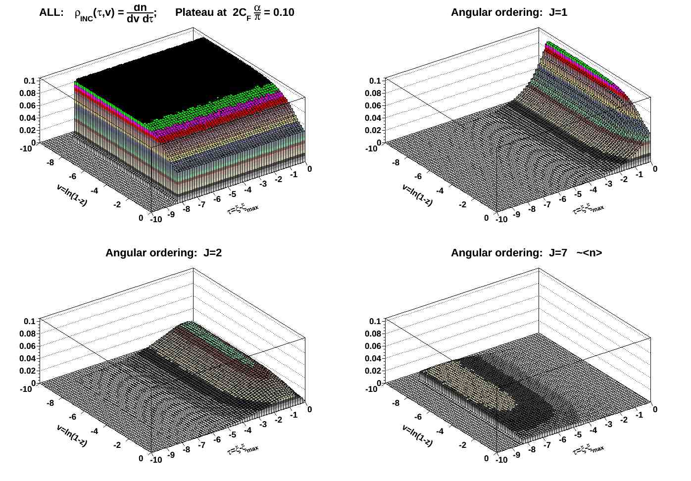
Figure 7: The distribution of gluons ordered in rapidity, as in our basic LO MC.

The reason why POWHEG technique is complicated in case of the angular ordering is illustrated in Fig. 7. We show there the distribution of gluons ordered in rapidity, starting from the gluon with the maximum rapidity, the closest to hard process. The gluon distribution with the highest rapidity $\xi\sim\xi_{\max}$ ($J=1$) has a ridge extending towards the soft region. Notice that, when the IR cut-off $\epsilon\to 0$ in $(1-z)<\epsilon$, the width of this ridge also goes to zero. Consequently, the gluon with the highest $\xi$ is unable to reproduce the gluon distribution in the NLO corner, close to hard process. This is why in this case POWHEG requires truncated and vetoed showers, which are not needed in our method.

5 Summary and outlook

A new method of adding the QCD NLO corrections to the hard process in the initial state Monte Carlo parton shower is tested numerically showing that the basic concept of the new methodology works correctly in the numerical environment of a Monte Carlo parton shower. The differences with the well established methods of MC@NLO and POWHEG are briefly discussed. Also, variants of the new method with better efficiency in terms of CPU time are proposed.

References

-
[1]
D. J. Gross and F. Wilczek, Phys. Rev. Lett. 30 (1973) 1343;
H. D. Politzer, Phys. Rev. Lett. 30 (1973) 1346;
D. J. Gross and F. Wilczek, Phys. Rev. D8 (1973) 3633;
H. D. Politzer, Phys. Rep. 14 (1974) 129. - [2] D. J. Gross and F. Wilczek, Asymptotically Free Gauge Theories. 2, Phys. Rev. D9 (1974) 980–993.
- [3] H. Georgi and H. D. Politzer, Electroproduction scaling in an asymptotically free theory of strong interactions, Phys. Rev. D9 (1974) 416–420.
- [4] S. Jadach, A. Kusina, W. Placzek, M. Skrzypek, and M. Slawinska, On the inclusion of the QCD NLO corrections in the quark– gluon Monte Carlo shower, 1103.5015.
- [5] S. Jadach, M. Jezabek, A. Kusina, W. Placzek, and M. Skrzypek, NLO corrections to hard process in QCD shower – proof of concept, 1209.4291.
- [6] S. Jadach, A. Kusina, and Skrzypek, NLO corrections to ladder part of the initial state shower in QCD, 2012. Report IFJPAN-IV-2012-7, in preparation.
- [7] S. Jadach, Foam: A general purpose cellular Monte Carlo event generator, Comput. Phys. Commun. 152 (2003) 55–100, [physics/0203033].
- [8] S. Jadach, W. Placzek, M. Skrzypek, and P. Stoklosa, Markovian Monte Carlo program EvolFMC v.2 for solving QCD evolution equations, Comput. Phys. Commun. 181 (2010) 393–412, [0812.3299].
- [9] K. Golec-Biernat, S. Jadach, W. Płaczek, and M. Skrzypek, Markovian Monte Carlo solutions of the NLO QCD evolution equations, Acta Phys. Polon. B37 (2006) 1785–1832, [hep-ph/0603031].
- [10] S. Jadach, W. Placzek, M. Skrzypek, P. Stephens, and Z. Was, Constrained MC for QCD evolution with rapidity ordering and minimum kT*, Comput.Phys.Commun. 180 (2009) 675–698, [hep-ph/0703281].
- [11] T. Sjostrand, A model for initial state parton showers, Phys. Lett. B157 (1985) 321.
- [12] F. A. Berends and R. Kleiss, Initial State Radiation for e+ e- Annihilation Into Jets, Nucl.Phys. B178 (1981) 141.
- [13] S. Alioli, K. Hamilton, and E. Re, Practical improvements and merging of POWHEG simulations for vector boson production, JHEP 1109 (2011) 104, [1108.0909].
- [14] S. Frixione and B. R. Webber, Matching NLO QCD computations and parton shower simulations, JHEP 06 (2002) 029, [hep-ph/0204244].
- [15] P. Nason, A new method for combining NLO QCD with shower Monte Carlo algorithms, JHEP 11 (2004) 040, [hep-ph/0409146].
- [16] S. Frixione, P. Nason, and C. Oleari, Matching NLO QCD computations with Parton Shower simulations: the POWHEG method, JHEP 0711 (2007) 070, [0709.2092].