Radiative natural supersymmetry
with mixed axion/higgsino cold dark matter

Abstract

Models of natural supersymmetry seek to solve the little hierarchy problem by positing a spectrum of light higgsinos $\stackrel{{\scriptstyle<}}{{\sim}}200$ GeV and light top squarks $\stackrel{{\scriptstyle<}}{{\sim}}500$ GeV along with very heavy squarks and TeV-scale gluinos. Such models have low electroweak finetuning and are safe from LHC searches. However, in the context of the MSSM, they predict too low a value of $m_{h}$ and the relic density of thermally produced higgsino-like WIMPs falls well below dark matter (DM) measurements. Allowing for high scale soft SUSY breaking Higgs mass $m_{H_{u}}>m_{0}$ leads to natural cancellations during RG running, and to radiatively induced low finetuning at the electroweak scale. This model of radiative natural SUSY (RNS), with large mixing in the top squark sector, allows for finetuning at the 5-10% level with TeV-scale top squarks and a 125 GeV light Higgs scalar $h$. If the strong CP problem is solved via the PQ mechanism, then we expect an axion-higgsino admixture of dark matter, where either or both the DM particles might be directly detected.

I Introduction

The recent fabulous discovery by Atlas and CMS of a Higgs-like resonance at 125 GeVatlas_h ; cms_h adds credence to supersymmetric models (SUSY) of particle physics in that the mass value falls squarely within the narrow predicted MSSM window: $m_{h}\sim 115-135$ GeVmhiggs . At the same time, a lack of a SUSY signal at LHC7 and LHC8 implies squarks and gluinos beyond the 1 TeV rangeatlas_susy ; cms_susy , exacerbating the little hierarchy problem (LHP):

• how do multi-TeV values of SUSY model parameters conspire to yield a $Z$-boson mass of just 91.2 GeV?

Models of natural supersymmetrykn address the LHP by positing a spectrum of light higgsinos $\stackrel{{\scriptstyle<}}{{\sim}}200$ GeV and light top squarks $\stackrel{{\scriptstyle<}}{{\sim}}500$ GeV along with very heavy first/second generation squarks and TeV-scale gluinosah ; others ; bbht . Such a spectrum allows for low electroweak finetuning while at the same time keeping sparticles safely beyond LHC search limits. In these models, the radiative corrections to $m_{h}$, which increase with $m_{\tilde{t}_{i}}^{2}$, are somewhat suppressed and have great difficulty in generating a light SUSY Higgs scalar with mass $m_{h}\sim 125$ GeVh125 . Thus, we are faced with a new conundrum: how do we reconcile low electroweak finetuning with such a large value of $m_{h}$hpr ? In addition, the light higgsino-like WIMP particles predicted by models of natural SUSY lead to a thermally-generated relic density which is typically a factor 10-15 belowbbh ; bbht the WMAP measured value of $\Omega_{CDM}h^{2}\simeq 0.11$.

One solution to the finetuning/Higgs problem is to add extra matter to the theory, thus moving beyond the MSSMhpr . For example, adding an extra singlet as in the NMSSM adds further quartic terms to the higgs potential thus allowing for increased values of $m_{h}$nmssm . One may also add extra vector-like matter to increase $m_{h}$ while maintaining light top squarksvecmatter . In the former case of the NMSSM, adding extra gauge singlets may lead to re-introduction of destabilizing divergences into the theorybpr . In the latter case, one might wonder about the ad-hoc introduction of extra weak scale matter multiplets and how they might have avoided detection A third possibility, which is presented below, is to re-examine EWFT and to ascertain if there do exist sparticle spectra within the MSSM that lead to $m_{h}\sim 125$ GeV while maintaining modest levels of electroweak finetuning.

II Electroweak finetuning

One way to evaluate EWFT in SUSY models is to examine the minimization condition on the Higgs sector scalar potential which determines the $Z$ boson mass. (Equivalently, one may examine the mass formula for $m_{h}$ and draw similar conclusions.) One obtains the well-known tree-level expression

$$\frac{m_{Z}^{2}}{2}=\frac{m_{H_{d}}^{2}-m_{H_{u}}^{2}\tan^{2}\beta}{\tan^{2}\beta-1}-\mu^{2}\;.$$ (1)

To obtain a natural value of $M_{Z}$ on the left-hand-side, one would like each term $C_{i}$ (with $i=H_{d},\ H_{u}$ and $\mu$) on the right-hand-side to be of order $m_{Z}^{2}/2$. This leads to a finetuning parameter definition

$$\Delta\equiv max_{i}\left(C_{i}\right)/(m_{Z}^{2}/2)$$ (2)

where $C_{H_{u}}=|-m_{H_{u}}^{2}\tan^{2}\beta/(\tan^{2}\beta-1)|/$, $C_{H_{d}}=|m_{H_{d}}^{2}/(\tan^{2}\beta-1)|/$ and $C_{\mu}=|-\mu^{2}|$ . Since $C_{H_{d}}$ is suppressed by $\tan^{2}\beta-1$, for even moderate $\tan\beta$ values this expression reduces approximately to

$$\frac{m_{Z}^{2}}{2}\simeq-m_{H_{u}}^{2}-\mu^{2}.$$ (3)

The question then arises: what is the model, what are the input parameters, and how do we interpret Eq’s 1 and 3?

Suppose we have a model with input parameters defined at some high scale $\Lambda\gg m_{SUSY}$, where $m_{SUSY}$ is the SUSY breaking scale $\sim 1$ TeV. Then

$$m_{H_{u}}^{2}(m_{SUSY})=m_{H_{u}}^{2}(\Lambda)+\delta m_{H_{u}}^{2}$$ (4)

where

$$\delta m_{H_{u}}^{2}\simeq-\frac{3f_{t}^{2}}{8\pi^{2}}\left(m_{Q_{3}}^{2}+m_{U_{3}}^{2}+A_{t}^{2}\right)\ln\left(\frac{\Lambda}{m_{SUSY}}\right).$$ (5)

The usual lore is that in a model defined at energy scale $\Lambda$, then both $m_{H_{u}}^{2}(\Lambda)$ and $\delta m_{H_{u}}^{2}$ must be of order $m_{Z}^{2}/2$ in order to avoid finetuning. In fact, requiring $\delta m_{H_{u}}^{2}\stackrel{{\scriptstyle<}}{{\sim}}m_{Z}^{2}/2$ has been used to argue for a sparticle mass spectra of natural SUSY. Taking $\Delta=10$ corresponds to

• $|\mu|\stackrel{{\scriptstyle<}}{{\sim}}200\ {\rm GeV}$,

• $m_{\tilde{t}_{i}},\ m_{\tilde{b}_{1}}\stackrel{{\scriptstyle<}}{{\sim}}500\ {\rm GeV}$,

• $m_{\tilde{g}}\stackrel{{\scriptstyle<}}{{\sim}}1.5\ {\rm TeV}$.

Since first/second generation squarks and sleptons hardly enter into Eq. 1, these can be much heavier: beyond LHC reach and also possibly providing a (partial) decoupling solution to the SUSY flavor and CP problems:

• $m_{\tilde{q},\tilde{\ell}}\sim 10-50$ TeV.

The natural SUSY solution reconciles lack of a SUSY signal at LHC with allowing for electroweak naturalness. It also predicts that the $\tilde{t}_{1,2}$ and $\tilde{b}_{1}$ may soon be accessible to LHC searches. New limits from direct top and bottom squark pair production searches, interpreted within the context of simplified models, are biting into the NS parameter spacelhc_stop . Of course, if $m_{\tilde{t}_{1,2}},\ m_{\tilde{b}_{1}}\simeq m_{\widetilde{Z}_{1}}$, then the visible decay products from stop and sbottom production will be soft and difficult to see at LHC. A more worrisome problem is that, with such light top squarks, the radiative corrections to $m_{h}$ are not large enough to yield $m_{h}\simeq 125$ GeV. This problem has been used to argue that additional multiplets beyond those of the MSSM must be present in order to raise up $m_{h}$ while maintaining very light third generation squarkshpr . A third issue is that the relic abundance of higgsino-like WIMPs, calculated in the standard MSSM-only cosmology, is typically a factor 10-15 below measured values. These issues have led some people to grow increasingly skeptical of weak scale SUSY, even as occurs in the natural SUSY incarnation.

One resolution to the above finetuning problem is to merely invoke a SUSY particle spectrum at the weak scale, as in the pMSSM model. Here, $\Lambda\sim m_{SUSY}$ so $\delta m_{H_{u}}^{2}\sim 0$ and we may select parameters $m_{H_{u}}^{2}\sim\mu^{2}\sim m_{Z}^{2}$. While a logical possibility, this solution avoids the many attractive features of a model which is valid up to a high scale such as $\Lambda\sim m_{GUT}$, with gauge coupling unification and radiative electroweak symmetry breaking driven by a large top quark mass.

Another resolution is to impose Eq. 1 as a condition on high scale models, but using only weak scale parameters. In this case, we will differentiate the finetuning measure as $\Delta_{EW}$, while the finetuning measure calculated using high scale input parameters we will refer to as $\Delta_{HS}$. The weaker condition of allowing only for $\Delta_{EW}\stackrel{{\scriptstyle<}}{{\sim}}20$ allows for possible cancellations in $m_{H_{u}}^{2}(m_{SUSY})$. This is precisely what happens in what is known as the hyperbolic branch or focus point region of mSUGRAhb_fp : $m_{H_{u}}^{2}(\Lambda)\simeq-\delta m_{H_{u}}^{2}\sim m_{Z}^{2}$ and consequently a value of $\mu^{2}\sim m_{Z}^{2}$ is chosen to enforce the measured value of $m_{Z}$ from Eq. 1. The HB/FP region of mSUGRA occurs for small values of trilinear soft parameter $A_{0}$. Small $A_{0}$ leads to small $A_{t}$ at the weak scale, which leads to $m_{h}\sim 115-120$ GeV, well below the Atlas/CMS measured value of $m_{h}\simeq 125$ GeV. Scans over parameter space show the HB/FP region is nearly excluded if one requires both low $|\mu|\sim m_{Z}$ and $m_{h}\sim 123-127$ GeVbbm2 ; sug .

The cancellation mechanism can also be seen from an approximate analytic solution of the EWSB minimation by Kane et al.kane :

$$m_{Z}^{2}\simeq = -1.8\mu^{2}+5.9M_{3}^{2}-0.4M_{2}^{2}-1.2m_{H_{u}}^{2}+0.9m_{Q_{3}}^{2}$$ (6)

$$+0.7m_{U_{3}}^{2}-0.6A_{t}M_{3}+0.4M_{2}M_{3}+\cdots$$

(which adopts $\tan\beta=5$ although similar expressions may be gained for other $\tan\beta$ values). All parameters on the RHS are GUT scale parameters. We see one solution for obtaining $m_{Z}$ on the left-hand side is to have all GUT scale parameters of order $m_{Z}$ (this is now excluded by recent LHC limits). The other possibility– if some terms are large (like $M_{3}\stackrel{{\scriptstyle>}}{{\sim}}0.4$ TeV in accord with recent LHC limits)– is to have large cancellations. The simplest possibility– using $M_{3}\stackrel{{\scriptstyle>}}{{\sim}}0.4$ TeV– is then to raise up $m_{H_{u}}^{2}$ beyond $m_{0}$ such that there is a large cancellation. This possibility is allowed in the non-universal Higgs modelsnuhm2 ; nuhm1 .

In mSUGRA, the condition that $m_{H_{u}}^{2}=m_{H_{d}}^{2}=m_{\tilde{q}}^{2}=m_{\tilde{\ell}}^{2}\equiv m_{0}^{2}$ at the high scale is anyways hard to accept. One might expect that all matter scalars in each generation are nearly degenerate since the known matter in each generation fills out complete 16-dimensional representations of $SO(10)$. However, the distinguishing feature of the Higgs multiplets is that they would live in 10-dimensional representations, and we then would not expect $m_{10}=m_{16}$ at $m_{GUT}$. A more likely choice would be to move to the non-universal Higgs model, which comes in several varieties. It was shown in Ref. nuhm1 that by adopting a simple one-parameter extension of mSUGRA– known as the one extra parameter non-universal Higgs model (NUHM1), with parameter space

$$m_{H_{u}}^{2}=m_{H_{d}}^{2}\equiv m_{\phi}^{2},\ m_{0},\ m_{1/2},\ A_{0},\ \tan\beta,\ sign(\mu)$$ (7)

– then for any spectra one may raise $m_{\phi}$ up beyond $m_{0}$ until at some point $m_{H_{u}}^{2}(m_{SUSY})$ drops in magnitude to $\sim m_{Z}^{2}$. The EWSB minimization condition then also forces $|\mu|\sim m_{Z}$. The worst of the EWFT is eliminated due to a large cancellation between $m_{H_{u}}^{2}(\Lambda=m_{GUT})$ and $\delta m_{H_{u}}^{2}$ leading to low $\Delta_{EW}$ and a model which enjoys electroweak naturalness.

The cancellation obviously can also be implemented in the 2-extra-parameter model NUHM2 where both $m_{H_{u}}^{2}(m_{GUT})$ and $m_{H_{d}}^{2}(m_{GUT})$ may be taken as free parameters (as in an $SU(5)$ SUSY GUT) or– using the EWSB minimization conditions– these may be traded for weak scale values of $\mu$ and $m_{A}$ as alternative inputsnuhm2 . A third possibility that will allow for an improved decoupling solution to the SUSY flavor and CP problems would occur if we allow for split generations $m_{0}(3)$ and $m_{0}(1)\simeq m_{0}(2)\equiv m_{0}(1,2)$ (SGNUHM). The latter condition need not require exact degeneracy, since with $m_{0}(1)\sim m_{0}(2)\sim 10-20$ TeV we obtain only a partial decoupling solution to the flavor problem. Taking $m_{0}(1,2)\sim 10-20$ TeV solves the SUSY CP problemsusyflcp .

III Radiative natural SUSY

Motivated by the possibility of cancellations occuring in $m_{H_{u}}^{2}(m_{SUSY})$, we go back to the EWSB minimization condition and augment it with radiative corrections $\Sigma_{u}^{u}$ and $\Sigma_{d}^{d}$ since if $m_{H_{u}}^{2}$ and $\mu^{2}$ are suppressed, then these may dominate:

$$\frac{m_{Z}^{2}}{2}=\frac{(m_{H_{d}}^{2}+\Sigma_{d}^{d})-(m_{H_{u}}^{2}+\Sigma_{u}^{u})\tan^{2}\beta}{\tan^{2}\beta-1}-\mu^{2}\;.$$ (8)

Here the $\Sigma_{u}^{u}$ and $\Sigma_{d}^{d}$ terms arise from derivatives of the radiatively corrected Higgs potential evaluated at the potential minimum. At the one-loop level, $\Sigma_{u}^{u}$ contains the contributionsan $\Sigma_{u}^{u}(\tilde{t}_{1,2})$, $\Sigma_{u}^{u}(\tilde{b}_{1,2})$, $\Sigma_{u}^{u}(\tilde{\tau}_{1,2})$, $\Sigma_{u}^{u}(\widetilde{W}_{1,2})$, $\Sigma_{u}^{u}(\widetilde{Z}_{1-4})$, $\Sigma_{u}^{u}(h,H)$, $\Sigma_{u}^{u}(H^{\pm})$, $\Sigma_{u}^{u}(W^{\pm})$, $\Sigma_{u}^{u}(Z)$, and $\Sigma_{u}^{u}(t)$. $\Sigma_{d}^{d}$ contains similar terms along with $\Sigma_{d}^{d}(b)$ and $\Sigma_{d}^{d}(\tau)$ while $\Sigma_{d}^{d}(t)=0$ bbhmmt . There are also contributions from $D$-term contributions to first/second generation squarks and sleptons which nearly cancel amongst themselves (due to sum of weak isospins/hypercharges equaling zero). Once we are in parameter space where $m_{H_{u}}^{2}(m_{SUSY})\sim\mu^{2}\sim m_{Z}^{2}$, then the radiative corrections $\Sigma_{u}^{u}$ may give the largest contribution to $\Delta_{EW}$.

The largest of the $\Sigma_{u}^{u}$ almost always come from top squarks, where we find

$$\Sigma_{u}^{u}(\tilde{t}_{1,2}) = \frac{3}{16\pi^{2}}F(m_{\tilde{t}_{1,2}}^{2})\times$$ (9)

$$\left[f_{t}^{2}-g_{Z}^{2}\mp\frac{f_{t}^{2}A_{t}^{2}-8g_{Z}^{2}(\frac{1}{4}-\frac{2}{3}x_{W})\Delta_{t}}{m_{\tilde{t}_{2}}^{2}-m_{\tilde{t}_{1}}^{2}}\right]$$

where $\Delta_{t}=(m_{\tilde{t}_{L}}^{2}-m_{\tilde{t}_{R}}^{2})/2+m_{Z}^{2}\cos 2\beta(\frac{1}{4}-\frac{2}{3}x_{W})$, $g_{Z}^{2}=(g^{2}+g^{\prime 2})/8$, $x_{W}\equiv\sin^{2}\theta_{W}$ and $F(m^{2})=m^{2}\left(\log(m^{2}/Q^{2})-1\right)$. In Ref. ltr , it is shown that for the case of the $\tilde{t}_{1}$ contribution, as $|A_{t}|$ gets large there is a suppression of $\Sigma_{u}^{u}(\tilde{t}_{1})$ due to a cancellation between terms in the square brackets of Eq. (9). For the $\tilde{t}_{2}$ contribution, a large splitting between $m_{\tilde{t}_{2}}$ and $m_{\tilde{t}_{1}}$ yields a large cancellation within $F(m_{\tilde{t}_{2}}^{2})$ $\left(\log(m_{\tilde{t}_{2}}^{2}/Q^{2})\rightarrow\log(m_{\tilde{t}_{2}}/m_{\tilde{t}_{1}})\rightarrow 1\right)$ for $Q^{2}=m_{\tilde{t}_{1}}m_{\tilde{t}_{2}}$, leading also to suppression. So while large $|A_{t}|$ values suppress both top squark contributions to $\Sigma_{u}^{u}$, at the same time they also lift up the value of $m_{h}$, which is near maximal for large, negative $A_{t}$. Combining all effects, one sees that the same mechanism responsible for boosting the value of $m_{h}$ into accord with LHC measurements can also suppress the $\Sigma_{u}^{u}$ contributions to EWFT, leading to a model with electroweak naturalness.

To illustrate these ideas, we adopt a simple benchmark point from the 2-parameter non-universal Higgs mass SUSY model NUHM2nuhm2 , but with split generations, where $m_{0}(3)<m_{0}(1,2)$. In Fig. 1, we take $m_{0}(3)=5$ TeV, $m_{0}(1,2)=10$ TeV, $m_{1/2}=700$ GeV, $\tan\beta=10$ with $\mu=150$ GeV, $m_{A}=1000$ GeV and $m_{t}=173.2$ GeV. We allow the GUT scale parameter $A_{0}$ to vary, and calculate the sparticle mass spectrum using Isajet 7.83isajet , which includes the new EWFT measure. In frame a), we plot the value of $m_{h}$ versus $A_{0}$. While for $A_{0}\sim 0$ the value of $m_{h}\sim 120$ GeV, as $A_{0}$ moves towards $-2m_{0}(3)$, the top squark radiative contributions to $m_{h}$ increase, pushing its value up to 125 GeV. (There is an expected theory error of $\pm 2$ GeV in our RGE-improved effective potential calculation of $m_{h}$, which includes leading 2-loop effectshh .) At the same time, in frame b), we see the values of $m_{\tilde{t}_{1,2}}$ versus $A_{0}$. In this case, large values of $A_{0}$ suppress the soft terms $m_{Q_{3}}^{2}$ and $m_{U_{3}}^{2}$ via RGE running. But also large weak scale values of $A_{t}$ provide large mixing in the top squark mass matrix which suppresses $m_{\tilde{t}_{1}}$ and leads to an increased splitting between the two mass eigenstates which suppresses the top squark radiative corrections $\Sigma_{u}^{u}(\tilde{t}_{2})$. The EWFT measure $\Delta\equiv\Delta_{EW}$ is shown in frame c), where we see that while $\Delta\sim 50$ for $A_{0}=0$, when $A_{0}$ becomes large, then $\Delta$ drops to 10, or $\Delta^{-1}=10\%$ EWFT. In frame d), we show the weak scale value of $A_{t}$ versus $A_{0}$ variation. While the EWFT is quite low– in the range expected for natural SUSY models– we note that the top squark masses remain above the TeV level, and in particular $m_{\tilde{t}_{2}}\sim 3.5$ TeV, in contrast to previous natural SUSY expectations.

Figure 1: Plot of a) $m_{h}$, b) $m_{\tilde{t}_{1,2}}$, c) $\Delta$ and d) $A_{t}$ versus variation in $A_{0}$ for a model with $m_{0}(1,2)=10$ TeV, $m_{0}(3)=5$ TeV, $m_{1/2}=700$ GeV, $\tan\beta=10$ and $\mu=150$ GeV and $m_{A}=1$ TeV.

IV Sparticle spectrum

The sparticle mass spectrum for this radiative NS benchmark point (RNS1) is shown in Table 1 for $A_{0}=-7300$ GeV. The heavier spectrum of top and bottom squarks seem likely outside of any near-term LHC reach, although in this case gluinobblt and possibly heavy electroweak-inowh pair production may be accessible to LHC14. Dialing the $A_{0}$ parameter up to $-8$ TeV allows for $m_{h}=125.2$ GeV but increases EWFT to $\Delta=29.5$, or 3.4% fine-tuning. Alternatively, pushing $m_{t}$ up to 174.4 GeV increases $m_{h}$ to $124.5$ GeV with 6.2% fine-tuning; increasing $\tan\beta$ to 20 increases $m_{h}$ to 124.6 GeV with 3.3% fine-tuning. We show a second point RNS2 with $m_{0}(1,2)=m_{0}(3)=7.0$ TeV and $\Delta=11.5$ with $m_{h}=125$ GeV; note the common sfermion mass parameter at the high scale. For comparison, we also show in Table 1 the NS2 benchmark from Ref. bbht ; in this case, a more conventional light spectra of top squarks is generated leading to $m_{h}=121.1$ GeV, but the model– with $\Delta=23.7$– has higher EWFT than RNS1 or RNS2.

parameter	RNS1	RNS2	NS2
$m_{0}(1,2)$	10000	7025.0	19542.2
$m_{0}(3)$	5000	7025.0	2430.6
$m_{1/2}$	700	568.3	1549.3
$A_{0}$	-7300	-11426.6	873.2
$\tan\beta$	10	8.55	22.1
$\mu$	150	150	150
$m_{A}$	1000	1000	1652.7
$m_{\tilde{g}}$	1859.0	1562.8	3696.8
$m_{\tilde{u}_{L}}$	10050.9	7020.9	19736.2
$m_{\tilde{u}_{R}}$	10141.6	7256.2	19762.6
$m_{\tilde{e}_{R}}$	9909.9	6755.4	19537.2
$m_{\tilde{t}_{1}}$	1415.9	1843.4	572.0
$m_{\tilde{t}_{2}}$	3424.8	4921.4	715.4
$m_{\tilde{b}_{1}}$	3450.1	4962.6	497.3
$m_{\tilde{b}_{2}}$	4823.6	6914.9	1723.8
$m_{\tilde{\tau}_{1}}$	4737.5	6679.4	2084.7
$m_{\tilde{\tau}_{2}}$	5020.7	7116.9	2189.1
$m_{\tilde{\nu}_{\tau}}$	5000.1	7128.3	2061.8
$m_{\widetilde{W}_{2}}$	621.3	513.9	1341.2
$m_{\widetilde{W}_{1}}$	154.2	152.7	156.1
$m_{\widetilde{Z}_{4}}$	631.2	525.2	1340.4
$m_{\widetilde{Z}_{3}}$	323.3	268.8	698.8
$m_{\widetilde{Z}_{2}}$	158.5	159.2	156.2
$m_{\widetilde{Z}_{1}}$	140.0	135.4	149.2
$m_{h}$	123.7	125.0	121.1
$\Omega_{\widetilde{Z}_{1}}^{std}h^{2}$	0.009	0.01	0.006
$BF(b\rightarrow s\gamma)\times 10^{4}$	$3.3$	3.3	$3.6$
$BF(B_{s}\rightarrow\mu^{+}\mu^{-})\times 10^{9}$	$3.8$	3.8	$4.0$
$\sigma^{SI}(\widetilde{Z}_{1}p)$ (pb)	$1.1\times 10^{-8}$	$1.7\times 10^{-8}$	$1.8\times 10^{-9}$
$\Delta$	9.7	11.5	23.7

Table 1: Input parameters and masses in GeV units for two radiative natural SUSY benchmark points and one NS point with $\mu=150$ GeV and $m_{t}=173.2$ GeV.

The RNS model shares some features of generic NS models, but also includes important differences. The several benchmark points shown in Table 1 imply that RNS is characterized by:

• a higgsino mass $\mu\sim M_{Z}\sim 100-300$ GeV,

• a light top squark $m_{\tilde{t}_{1}}\sim 1-2$ TeV,

• a heavier top-squark $m_{\tilde{t}_{2}}\sim em_{\tilde{t}_{1}}\sim 2-4$ TeV (here, $e\equiv 2.718...$),

• $m_{\tilde{g}}\sim 1-5$ TeV,

• first/second generation sfermions $\sim 5-20$ TeV.

While $\mu\sim m_{Z}$ as in usual NS models, the heavier top squarks and gluinos implied by RNS allow for $m_{h}\simeq 125$ GeV but may make this model more difficult to detect at LHC than usual NS.

To illustrate how low EWFT comes about even with rather heavy top squarks, we show in Fig. 2 the various third generation contributions to $\Sigma_{u}^{u}$, where the lighter mass eigenstates are shown as solid curves, while heavier eigenstates are dashed. The sum of all contributions to $\Sigma_{u}^{u}$ is shown by the black curve marked total. From the figure we see that for $A_{0}\sim 0$, indeed both top squark contributions to $\Sigma_{u}^{u}$ are large and negative, leading to a large value of $\Sigma_{u}^{u}(total)$, which will require large fine-tuning in Eq. (8). As $A_{0}$ gets large negative, both top squark contributions to $\Sigma_{u}^{u}$ are suppressed, and $\Sigma_{u}^{u}(\tilde{t}_{1})$ even changes sign, leading to cancellations amongst the various $\Sigma_{u}^{u}$ contributions.

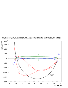
Figure 2: Plot of third generation contributions to $\Sigma_{u}^{u}$ versus $A_{0}$ for benchmark point RNS1 where solid curves come form the lighter mass eigenstate and dashed curves from the heavier. The black solid curve is $\Sigma_{u}^{u}$ which has summed over all contributions.

V Radiative natural SUSY at colliders:

What chance does LHC have of detecting RNS? Unlike previous NS models, RNS has top and bottom squarks more typically in the $m_{\tilde{t}_{1}}\sim 1-2$ TeV and $m_{\tilde{t}_{2}}\sim 2-4$ TeV range, likely beyond LHC reach. It also has light higgsinos $\widetilde{W}_{1}^{\pm}$, $\widetilde{Z}_{1,2}$. While these latter particles can have substantial production cross sections at LHC, the mass gaps $m_{\widetilde{W}_{1}}-m_{\widetilde{Z}_{1}}$ and $m_{\widetilde{Z}_{2}}-m_{\widetilde{Z}_{1}}$ are typically in the $10-50$ GeV range. Thus, the visible decay products from $\widetilde{W}_{1}^{+}\widetilde{W}_{1}^{-}$ and $\widetilde{W}_{1}^{\pm}\widetilde{Z}_{2}$ production tend to be at rather low energies, making observability difficult. The best bet may be if gluinos lie in the lower half of their expected range $m_{\tilde{g}}\sim 1-5$ TeV. In this case, $\tilde{g}\rightarrow tb\widetilde{W}_{1}$ or $t\bar{t}\widetilde{Z}_{i}$ decays occur, and one might expect an observable rate for $\tilde{g}\tilde{g}\rightarrow 4t+E_{T}^{miss}$ signals. A portion of these events will contain cascade decays to $\widetilde{Z}_{2}\rightarrow\widetilde{Z}_{1}\ell^{+}\ell^{-}$ and if the OS/SF dilepton pair can be reconstructed, then its distinctive invariant mass distribution bounded by $m_{\widetilde{Z}_{2}}-m_{\widetilde{Z}_{1}}$ may point to the presence of light higgsinos.

The hallmark of RNS and other NS models is the presence of light higgsinos with mass $m_{\widetilde{W}_{1}},\ m_{\widetilde{Z}_{1,2}}\stackrel{{\scriptstyle<}}{{\sim}}200-300$ GeV. In this case, a linear $e^{+}e^{-}$ collider operating with $\sqrt{s}\stackrel{{\scriptstyle>}}{{\sim}}2m_{\widetilde{W}_{1}}$ would be a higgsino factory in addition to a Higgs factorybbh ; bl ! The soft decay products from $\widetilde{W}_{1}\rightarrow\widetilde{Z}_{1}f\bar{f}^{\prime}$ decay are not problematic for detection at an ILC, and will even be boosted as $\sqrt{s}$ increases well beyond threshold energy for creating charginos pairs. The reaction $e^{+}e^{-}\rightarrow\widetilde{Z}_{1}\widetilde{Z}_{2}$ will also be distinctive.

VI Mixed axion-higgsino cold dark matter:

In $R$-parity conserving SUSY models with higgsino-like WIMPsbbh , the relic density is usually a factor $10-15$ below the WMAP measured value of $\Omega_{CDM}h^{2}\simeq 0.11$. This is due to a high rate of higgsino annihilation into $WW$ and $ZZ$ final states in the early universe. Thus, the usual picture of thermally produced WIMP-only dark matter is inadequate for the case of models with higgsino-like WIMPs.

A variety of non-standard cosmological models have been proposed which can ameliorate this situation. For instance, at least one relatively light modulus field is expected from string theoryacharya , and if the scalar field decays after neutralino freeze-out with a substantial branching fraction into SUSY particles then it will typically augment the neutralino abundancemr .

Alternatively, or in addition, if the strong $CP$ problem is solved by the Peccei-Quinn mechanism in a SUSY context, then we expect the presence of axions in addition to $R$-parity odd spin $\frac{1}{2}$ axinos $\tilde{a}$ and $R$-parity even spin-0 saxions $s$. In this case, dark matter could consist of two particles: an axion-higgsino admixtureckls ; blrs ; bls . The neutralinos are produced thermally as usual, but are also produced via thermal production followed by cascade decays of axinos at high $T_{R}$. The late decay of axinos into higgsinos can cause a re-annihilation of neutralinos at temperatures below freeze-out, substantially augmenting the relic abundance. In addition, saxions can be produced both thermally at lower range of PQ breaking parameter $f_{a}$, and via coherent oscillations at high $f_{a}$, and in fact may temporarily dominate the energy density of the universe. Their decay $s\rightarrow aa$ is expected to dominate and would add to the measured $N_{eff}(\nu)$. Their decay $s\rightarrow\tilde{g}\tilde{g}$ or $\tilde{a}\tilde{a}$ would augment the neutralino abundance, while late decays into SM particles such as $gg$ would dilute all relics present at the time of decay. Exact dark matter abundances depend on the specific SUSY axion model and choices of PQMSSM parameters. It is possible one could have either axion or higgsino dominance of the relic abundance, or even a comparable mixture. In the latter case, it may be possible to directly detect both an axion and a higgsino-like WIMP.

VII Conclusions:

Models of Natural SUSY are attractive in that they enjoy low levels of EWFT, which arise from a low value of $\mu$ and possibly a sub-TeV spectrum of top squarks and $\tilde{b}_{1}$. In the context of the MSSM, such light top squarks are difficult to reconcile with the LHC Higgs boson discovery which requires $m_{h}\sim 125$ GeV. By imposing naturalness using $\Delta_{EW}$ with weak scale parameter inputs, we allow for large cancellations in $m_{H_{u}}^{2}$ as it is driven to the weak scale. In this case, for some range of $m_{H_{u}}^{2}(m_{GUT})>m_{0}$ (as in NUHM models), the weak scale value of $m_{H_{u}}^{2}$ will be $\sim m_{Z}^{2}$ thus generating the natural SUSY model radiatively. Models with a large negative trilinear soft-breaking parameter $A_{t}$ can maximize the value of $m_{h}$ into the $125$ GeV range without recourse to adding exotic matter into the theory. The large value of $A_{t}$ also suppresses 1-loop top squark contributions to the scalar potential minimization condition leading to models with low EWFT and a light Higgs scalar consistent with LHC measurements. (More details on the allowable parameter space of RNS will be presented in Ref. bbhmmt .) The large negative $A_{t}$ parameter can arise from large negative $A_{0}$ at the GUT scale.

While RNS may be difficult to detect at LHC unless gluinos, third generation squarks or the heavier electroweak-inos are fortuitously light, a linear $e^{+}e^{-}$ collider with $\sqrt{s}\stackrel{{\scriptstyle>}}{{\sim}}2|\mu|$ would have enough energy to produce the hallmark light higgsinos which are expected in this class of models. Since the model predicts a lower abundance of higgsino-like WIMP dark matter in the standard cosmology, there is room for mixed axion-higgsino cold dark matter. The axions are necessary anyway if one solves the strong $CP$ problem via the PQ mechanism.

- (1) G. Aad et al. [ATLAS Collaboration], Phys. Lett. B 716, 2012 (1).
- (2) S. Chatrchyan et al. [CMS Collaboration], Phys. Lett. B 716, 2012 (30).
- (3) M. S. Carena and H. E. Haber, Prog. Part. Nucl. Phys.50 (2003) 63 [hep-ph/0208209].
- (4) G. Aad et al. (ATLAS collaboration), Phys. Lett. B 710, 2012 (67).
- (5) S. Chatrchyan et al. (CMS collaboration), Phys. Rev. Lett. 1072011221804.
- (6) R. Kitano and Y. Nomura, Phys. Lett. B 631, 2005 (58) and Phys. Rev. D732006095004.
- (7) N. Arkani-Hamed, talk at WG2 meeting, Oct. 31, 2012, CERN, Geneva.
- (8) M. Papucci, J. T. Ruderman and A. Weiler, J. High Energy Phys. 1209, 2012 (035); C. Brust, A. Katz, S. Lawrence and R. Sundrum, J. High Energy Phys. 1203, 2012 (103); R. Essig, E. Izaguirre, J. Kaplan and J. G. Wacker, J. High Energy Phys. 1201, 2012 (074).
- (9) H. Baer, V. Barger, P. Huang and X. Tata, J. High Energy Phys. 1205, 2012 (109).
- (10) H. Baer, V. Barger and A. Mustafayev, Phys. Rev. D852012075010; H. Baer, V. Barger, P. Huang and A. Mustafayev, Phys. Rev. D842011091701.
- (11) L. Hall, D. Pinner and J. Ruderman, J. High Energy Phys. 1204, 2012 (131).
- (12) H. Baer, V. Barger and P. Huang, JHEP 1111 (2011) 031.
- (13) S. F. King, M. Muhlleitner and R. Nevzorov, Nucl. Phys. B 860 (2012) 207; J. F. Gunion, Y. Jiang and S. Kraml, Phys. Lett. B 710 (2012) 454; K. J. Bae, K. Choi, E. J. Chun, S. H. Im, C. B. Park and C. S. Shin, arXiv:1208.2555 [hep-ph].
- (14) S. P. Martin, Phys. Rev. D 81 (2010) 035004and Phys. Rev. D 82 (2010) 055019;K. J. Bae, T. H. Jung and H. D. Kim, arXiv:1208.3748 [hep-ph].
- (15) J. Bagger, E. Poppitz and L. Randall, Nucl. Phys. B 455 (1995) 59 [hep-ph/9505244].
- (16) G. Aad et al. [ATLAS Collaboration], arXiv:1209.2102 [hep-ex].
- (17) K. L. Chan, U. Chattopadhyay and P. Nath, Phys. Rev. D581998096004; J. Feng, K. Matchev and T. Moroi, Phys. Rev. Lett. 8420002322 and Phys. Rev. D612000075005; see also H. Baer, C. H. Chen, F. Paige and X. Tata, Phys. Rev. D5219952746 and Phys. Rev. D5319966241; H. Baer, C. H. Chen, M. Drees, F. Paige and X. Tata, Phys. Rev. D591999055014; for a model-independent approach, see H. Baer, T. Krupovnickas, S. Profumo and P. Ullio, J. High Energy Phys. 0510, 2005 (020).
- (18) O. Lebedev, H. P. Nilles and M. Ratz, hep-ph/0511320.
- (19) H. Baer, V. Barger and A. Mustafayev, JHEP 1205 (2012) 091.
- (20) H. Baer, V. Barger, P. Huang, D. Mickelson, A. Mustafayev and X. Tata, arXiv:1210.3019.
- (21) G. L. Kane, J. D. Lykken, B. D. Nelson and L. -T. Wang, Phys. Lett. B 551 (2003) 146.
- (22) J. Ellis, K. Olive and Y. Santoso, Phys. Lett. B 539, 2002 (107); J. Ellis, T. Falk, K. Olive and Y. Santoso, Nucl. Phys. B 652 (2003) 259; H. Baer, A. Mustafayev, S. Profumo, A. Belyaev and X. Tata, J. High Energy Phys. 0507, 2005 (065).
- (23) H. Baer, A. Mustafayev, S. Profumo, A. Belyaev and X. Tata, Phys. Rev. D712005095008
- (24) F. Gabbiani, E. Gabrielli, A. Masiero and L. Silvestrini, Nucl. Phys. B 477 (1996) 321.
- (25) R. Arnowitt and P. Nath, Phys. Rev. D4619923981.
- (26) H. Baer et al., in preparation.
- (27) H. Baer, V. Barger, P. Huang, A. Mustafayev and X. Tata, arXiv:1207.3343 [hep-ph].
- (28) ISAJET, by H. Baer, F. Paige, S. Protopopescu and X. Tata, hep-ph/0312045.
- (29) H. Haber and R. Hempfling, Phys. Rev. D4819934280.
- (30) H. Baer, V. Barger, A. Lessa and X. Tata, J. High Energy Phys. 1006, 2010 (102) and Phys. Rev. D852012051701.
- (31) H. Baer, V. Barger, A. Lessa, W. Sreethawong and X. Tata, Phys. Rev. D 85 (2012) 055022.
- (32) N. Arkani-Hamed and H. Murayama, Phys. Rev. D 56 (1997) 6733.
- (33) H. Baer, C. Balazs, P. Mercadante, X. Tata and Y. Wang, Phys. Rev. D 63 (2001) 015011.
- (34) H. Baer and J. List, arXiv:1205.6929 [hep-ph].
- (35) B. S. Acharya, G. Kane and E. Kuflik, arXiv:1006.3272 [hep-ph].
- (36) T. Moroi and L. Randall, Nucl. Phys. B 570 (2000) 455; G. Gelmini and P. Gondolo, Phys. Rev. D742006023510; G. Gelmini, P. Gondolo, A. Soldatenko and C. Yaguna, Phys. Rev. D742006083514; G. Gelmini, P. Gondolo, A. Soldatenko and C. Yaguna, Phys. Rev. D762007015010; B. Acharya, K. Bobkov, G. Kane, P. Kumar and J. Shao, Phys. Rev. D762007126010 and Phys. Rev. D782008065038; B. Acharya, P. Kumar, K. Bobkov, G. Kane, J. Shao and S. Watson, J. High Energy Phys. 0806, 2008 (064).
- (37) K-Y. Choi, J. E. Kim, H. M. Lee and O. Seto, Phys. Rev. D772008123501.
- (38) H. Baer, A. Lessa, S. Rajagopalan and W. Sreethawong, JCAP1106 (2011) 031.
- (39) H. Baer, A. Lessa and W. Sreethawong, JCAP1201 (2012) 036.