Top quark spin and $Htb$ interaction in charged Higgs and top quark associated production at LHC

Abstract

We study the charged Higgs production at LHC via its associated production with top quark. The kinematic cuts are optimized to suppress the background processes so that the reconstruction of the charged Higgs and top quark is possible. The angular distributions with respect to top quark spin are explored to study the $Htb$ interaction at LHC.

I Introduction

The Standard Model (SM) of particle physics, with great success, is based on two cornerstones: gauge symmetry and electroweak spontaneous symmetry breaking mechanism(EWSB). The gauge group $SU(3)_{C}\times SU(2)_{L}\times U(1)_{Y}$ of the SM has been confirmed by the discovery of $W/Z$ bosons and lots of precision measurements. As the other cornerstone, the mechanism of EWSB is implemented by introducing only one complex Higgs doublet $\Phi$ in the SM and then triggering EWSB after the neutral component of $\Phi$ developing a vacuum expectation value (vev). In the meanwhile, the masses of weak gauge bosons and fermions are generated. In the SM, there is only one physical neutral Higgs boson $H$ after EWSB. The discovery of the Higgs boson will help to unveil the mysteries of EWSB and mass generation of SM particles. Recently, one Higgs-like particle around 126 GeV has been discovered at LHC by ATLAS and CMS collaborationsHiggs_ATLAS ; Higgs_CMS . It is important to further confirm the identity of this particle. In the SM, only one complex scalar doublet is introduced based on the ”minimal principle”. It is natural to consider more complex scalars, for example, the two Higgs doublet structure. Especially, there are many motivations to study the two Higgs doublet model (2HDM). Such as, in the supersymmetric models, a single Higgs doublet is unable to give mass simultaneously to the charge 2/3 and charge -1/3 quarks and the anomaly cancellation also require an additional Higgs doublet. Another motivation for 2HDM is that it could generate a baryon asymmetry of the universe of sufficient size. Interestingly, ATLAS and CMS announced that there is an enhancement in the di-photon channel of Higgs decay $h\to\gamma\gamma$ Higgs_ATLAS ; Higgs_CMS . This enhancement can also be explained by charged Higgs from 2HDMcomprehensive .

There are many scenarios in 2HDM structure higgs hunter's guide ; 2hdm_review . Without imposing any discrete symmetry, the 2HDM suffers serious flavour changing neutral currents (FCNC) at tree-level. For the suppression of leading order FCNC as well as CP violation in the Higgs sector, we consider CP-conserving 2HDMs with extra discrete symmetry. Popular Type I and II 2HDMs belong to this kind. As one of the minimal extensions of the SM, 2HDMs higgs hunter's guide ; 2hdm_review , has five physical Higgs scalars after the spontaneous symmetry breaking, i.e., two neutral CP-even bosons $h_{0}$ and $H_{0}$, one neutral CP-odd boson $A$, and two charged bosons $H^{\pm}$. In diverse models, different scalar multiplets and singlets could generate neutral scalars and there exists mixing between neutral scalars which makes it difficult to unentangle the Higgs properties and confirm the existence of extended Higgs sector. However, the discovery of the charged Higgs boson could provide an unambiguous signature of the extended Higgs sector and help to further distinguish from different models.

Motivated by above reasons, the charged Higgs $H^{\pm}$ has been searched for at colliders in recent years. One model-independent direct limit is from the LEP experiments gives $M>78.6$ GeV at 95% C.L., where $M$ represents the mass of charged Higgs by exclusive decay channels of $H^{+}\to c\bar{s}$ and $H^{+}\to\tau^{+}\nu$LEP Higgs . At hadron colliders, the search approaches for the charged Higgs are different in low mass range $M<m_{t}$ and in large mass range $M>m_{t}$. In the low mass range $M<m_{t}-m_{b}$, the search for the signal mainly focus on the top quark decay $t\to H^{+}b$ followed by decay mode $H^{+}\to\bar{\tau}\nu$. On the other hand, for large mass range $M>m_{t}+m_{b}$, the signal is from the dominant production process, the $gb$ fusion process $gb\to tH^{-}$, followed by dominant decay modes $H^{-}\to t\bar{b}$ and $H^{-}\to\tau\bar{\nu}$. The Tevatron has put a constraint on 2HDM in the small $\tan\beta$ and large $\tan\beta$ regions for a charged Higgs boson with mass up to $\sim 160$ GeV Tevatron . In addition, the indirect constraints can be extracted from B-meson decays since the charged Higgs contributes to the FCNC at one loop level. In Type II 2HDM, a limit on the charged Higgs mass $M>316~{}{\rm GeV}$ at $95\%$ C.L. is obtained dominantly from $b\to s\gamma$ branching ratio measurement irrespective of the value of $\tan\beta$ typeII_constraints . However, in Type III or general 2HDM the phases of the Yukawa couplings are free parameters so that $M$ can be as low as 100 GeVbtosgamma1 . For more detailed discussions on phenomenological constraints on charged Higgs, we refer to Ref. PDG2012 .

Along with the experimental search for the charged Higgs boson, extensive phenomenological studies on charged Higgs boson production have been carried out collider higgs ; collider higgs2 ; dominate process ; tripleb ; fourb ; pt ; dominate process3 ; Kidonakis:2004ib . Especially, the $gb$ fusion process $gb\rightarrow tH^{-}$ for $M>m_{t}+m_{b}$ dominate process ; tripleb ; fourb ; pt ; dominate process3 ; Kidonakis:2004ib ; H+Jetsub has drawn more attentions due to the large couplings of $Htb$ interaction. The next-to-leading QCD corrections to this process has also been performed in order to make the theoretical predictions more reliableNLO .

In this work, we revisit this process at the LHC and take a method similar to Ref. Gopalakrishna:2010xm to distinguish the signal from backgrounds. As demonstrated in Ref. Gopalakrishna:2010xm , the angular distribution related to top quark spin is efficient to disentangle the chiral coupling of the $W^{\prime}$ boson to SM fermions. The left-right asymmetry induced by top quark spin for $pp\to tH^{-}$ process has been analyzed in Ref.Baglio:2011ap . Here we further investigate this kind of effects after including the decay information of charged Higgs and top quark, and we employ the angular distributions of the top quark and the lepton resulting from top and charged Higgs decay to disentangle $Htb$ couplings at LHC.

This paper is organized as follows. In Section II., the corresponding theoretical framework is briefly introduced. Section III. is devoted to the numerical analysis of top quark and charged Higgs associated production. Specifically, the correlated angular distributions are investigated to identify the interaction of top-bottom quark and charged Higgs. Finally, a short summary is given.

II Theoretical Framework

II.1 Lagrangian related to the interaction of Higgs and quarks

We start with a brief introduction to the two-Higgs-Doublet Model (2HDM) which is one of the minimal extensions of SM. Different from SM, 2HDM involves two complex ${SU(2)_{L}}$ doublet scalar fields.

$$\Phi_{i}=\left(\begin{array}[]{c}H_{i}^{+}\\ (H_{i}^{0}+iA_{i}^{0})/\sqrt{2}\end{array}\right),$$ (1)

where $i=1,2$. Imposing CP invariance and ${\rm U(1)_{EM}}$ gauge symmetry, the minimization of potential gives

$$\langle\Phi_{i}\rangle=\displaystyle{\frac{1}{\sqrt{2}}}\left(\begin{array}[]{c}0\\ v_{i}\end{array}\right),$$ (4)

with $v_{i}~{}(i=1,2)$ is non-zero vev. One important parameter in 2HDM ${\displaystyle{\tan\beta\equiv{v_{2}}/{v_{1}}}}$ is defined accordingly, which determines the interactions of the various Higgs fields with the vector bosons and fermions, it has substantial meaning in discussing phenomenology. The most severe constraints on $\tan\beta$ and $M$ come from flavour physics including $B$ and $D$ mesons, $\Delta M_{B_{d}}$, $b\to s\gamma$ and $Z\to b\bar{b}$typeII_constraints ; 2HDM_constraints . Large $\tan\beta$ is favored by $B$ meson rare decaysHewett:1992is ; Barger:1992dy ; Bertolini:1990if . Specifically, for the Type II model, the upper bound on $\tan\beta$ from $D_{s}\to\tau\nu_{\tau}$ is $\tan\beta\leq 50$ with charged Higgs mass $M=600$ GeV comprehensive .

In this work we aim to study the charged Higgs phenomenology with large $\tan\beta$ and choose the Type II Yukawa couplings as the working model

$$-\mathcal{L} = -\cot\beta\frac{m_{u}}{v}\bar{u}_{L}(H+iA)u_{R}$$ (5)

$$+\tan\beta\frac{m_{d}}{v}\bar{d}_{L}(H-iA)d_{R}$$

$$-\sqrt{2}\cot\beta\frac{m_{u}}{v}V_{ud}^{{\dagger}}\bar{d}_{L}H^{-}u_{R}$$

$$-\sqrt{2}\tan\beta\frac{m_{d}}{v}V_{ud}\bar{u}_{L}H^{+}d_{R}+{\rm h.c.}.$$

The vev of SM Higgs is related as $v=\sqrt{v_{1}^{2}+v_{2}^{2}}$. $t\bar{b}H^{-}$ vertex given in Ref.higgs hunter's guide can be written as

$$g_{H^{-}t\bar{b}} = g_{a}+g_{b}\gamma_{5}.$$ (6)

Within the type II 2HDM,

$$g_{a,b}=g({\rm cot}\beta m_{t}\pm{\rm tan}\beta m_{b})/(2\sqrt{2}m_{{\rm W}}).$$

In the specific discussions below in Sec. III, we will investigate various combinations of $(g_{a}g_{b})$ accordingly not limited in type II 2HDM.

II.2 Charged Higgs production associated with single top quark at hadron colliders

We begin to consider the following process(Fig. 1)

$$g(p_{1})+b(p_{2}) \to t(p_{3},s_{t})+H^{-}(p_{4})$$ (7)

$$\to t(p_{3},s_{t})+b(p_{5})+\bar{t}(p_{6},s_{\bar{t}}),$$

where $p_{i}$ denotes the 4-momentum of the corresponding particle. $s_{t}$($s_{\bar{t}}$) is the top(antitop) quark spin in 4-dimension and $s_{t}^{2}=s_{\bar{t}}^{2}=-1$, $p_{3}\cdot s_{t}=p_{6}\cdot s_{\bar{t}}=0$.

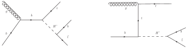
Figure 1: Feynman diagrams for $gb\to tH^{-}\to t\bar{t}b$ process.

Under the narrow width approximation of the charged Higgs, i.e., the charged Higgs is produced on-shell,

$$\lim_{\Gamma\to 0}\frac{1}{(p_{4}^{2}-M^{2})^{2}+\Gamma^{2}M^{2}}\longrightarrow\frac{\pi}{\Gamma M}\,\delta(p_{4}^{2}-M^{2}),$$ (8)

where $\Gamma$ and $M$ respectively denote the decay width and mass of the charged Higgs boson. The matrix element squared including top quark spin information for the process (7) can be written as follows

$$|{\cal M}(s_{t},s_{\bar{t}})|^{2}= |{\cal M}_{gb\to tH^{-}}(s_{t})|^{2}|{\cal M}_{H^{-}\to b\bar{t}}(s_{\bar{t}})|^{2}$$ (9)

$$\times\frac{\pi}{\Gamma M}\delta(p_{4}^{2}-M^{2}),$$

where

$$|{\cal M}_{gb\to tH^{-}}(s_{t})|^{2}=\frac{g_{s}^{2}}{2N_{c}}\Big{\{}{\cal A}+{\cal B}_{1}(p_{1}\cdot s_{t})+{\cal B}_{2}(p_{2}\cdot s_{\bar{t}})\Big{\}},$$ (10)

and

$$|{\cal M}_{H^{-}\to b\bar{t}}(s_{\bar{t}})|^{2} = (g_{a}^{2}+g_{b}^{2})(M^{2}-m_{b}^{2}-m_{t}^{2})$$ (11)

$$-2(g_{a}^{2}-g_{b}^{2})m_{b}m_{t}$$

$$-4g_{a}g_{b}m_{t}(p_{5}\cdot s_{\bar{t}}).$$

The formula for ${\cal A}$, ${\cal B}_{1}$ and ${\cal B}_{2}$ are listed in the following

$${\cal A}=(g_{a}^{2}+g_{b}^{2})\,A_{1}\,+\,m_{b}m_{t}(g_{b}^{2}-g_{a}^{2})\,A_{2},$$ (12)

with

$$A_{1} = \displaystyle{\frac{\hat{s}(p_{1}\cdot p_{3})-m_{b}^{2}(4p_{1}\cdot p_{3}+3p_{2}\cdot p_{3})}{(\hat{s}-m_{b}^{2})^{2}}}$$ (13)

$$+\frac{\hat{s}(p_{1}\cdot p_{3})+m_{t}^{2}(\hat{s}-2p_{2}\cdot p_{3})}{4(p_{1}\cdot p_{3})^{2}}$$

$$-\frac{1}{2(p_{1}\cdot p_{3})(\hat{s}-m_{b}^{2})}\big{\{}m_{t}^{2}(\hat{s}-2m_{b}^{2})-2(p_{1}\cdot p_{3})m_{b}^{2}$$

$$+2(\hat{s}-2p_{2}\cdot p_{3})(p_{1}\cdot p_{3}+p_{2}\cdot p_{3})\big{\}},$$

$$A_{2} = \frac{(\hat{s}+2m_{b}^{2})}{(\hat{s}-m_{b}^{2})^{2}}+\frac{m_{t}^{2}-p_{1}\cdot p_{3}}{2(p_{1}\cdot p_{3})^{2}}$$ (14)

$$-\frac{2p_{1}\cdot p_{3}+4p_{2}\cdot p_{3}-\hat{s}}{2(p_{1}\cdot p_{3})(\hat{s}-m_{b}^{2})},$$

and

$$B_{1} = 2g_{a}g_{b}m_{t}[\frac{4m_{b}^{2}-\hat{s}}{(\hat{s}-m_{b}^{2})^{2}}+\frac{2p_{2}\cdot p_{3}-\hat{s}}{4(p_{1}\cdot p_{3})^{2}}+\frac{1}{p_{1}\cdot p_{3}}$$ (15)

$$-\frac{p_{2}\cdot p_{3}}{(p_{1}\cdot p_{3})(\hat{s}-m_{b}^{2})}],$$

$$B_{2} = 2g_{a}g_{b}m_{t}[\frac{3m_{b}^{2}}{(\hat{s}-m_{b}^{2})^{2}}+\frac{m_{t}^{2}-p_{1}\cdot p_{3}}{2(p_{1}\cdot p_{3})^{2}}$$ (16)

$$+\frac{\hat{s}-p_{1}\cdot p_{3}-2p_{2}\cdot p_{3}}{(p_{1}\cdot p_{3})(\hat{s}-m_{b}^{2})}].$$

The matrix element squared for the process $g\bar{b}\to\bar{t}H^{+}\to t\bar{t}\bar{b}$ can be obtained from the above equations by using CP-invariance. Obviously, the top quark spin effects are related to the product $(g_{a}g_{b})$ and disappear for a pure scalar or pseudo-scalar charged Higgs boson. In particular, for $pp\to tH^{-}\to t\bar{t}b$ process, this feature can be reflected by the following spin observable

$$<{\cal{O}}_{t}>=2<\bf{{S_{t}}}\cdot{\bf\hat{a}}>={\sigma(\uparrow)-\sigma(\downarrow)\over\sigma(\uparrow)+\sigma(\downarrow)},\\$$ (17)

where $\bf{{S_{t}}}$ is top quark spin vector in its rest frame, and the arrows on the right-hand side refer to the spin state of the top quark with respect to the quantization axis ${\bf\hat{a}}$. At LHC, the helicity basis is a better choice, i.e., ${\bf\hat{a}}={\bf{\hat{p}}}_{t}^{*}$ with the unit 3-momentum ${\bf{\hat{p}}}_{t}^{*}$ in the $tH^{-}$ center-of-mass frame. Similarly, we can also define the spin observable with respect to antitop quark

$$<{\cal{O}}_{\bar{t}}>=2<\bf{{S}_{\bar{t}}}\cdot{\bf\hat{b}}>,$$ (18)

where $\bf{\hat{b}}$ is the spin quantization axis related to antitop quark. At LHC, we can choose ${\bf\hat{b}}={\bf{\hat{p}}}_{\bar{t}}^{*}$ with the unit 3-momentum ${\bf{\hat{p}}}_{\bar{t}}^{*}$ in the charged Higgs rest frame.

For the subsequent polarized top quark decay

$$t({\bf{S_{t}}})\to c(p_{c})+X,$$

where $c$ represents a final state particle or jet and $p_{c}$ is its momentum, the corresponding differential distribution is obtained as followsBrandenburg:2002xr

$$\frac{1}{\Gamma_{t}}\frac{d\Gamma_{t}}{d\cos\vartheta}=\frac{1}{2}\left(1+\kappa_{c}\cos\vartheta\right),$$ (19)

where $\vartheta$ is the angle between the top quark spin and the moving direction of $c$ in top quark rest frame. $\kappa_{c}$ is the so-called spin analysing power of the corresponding particle or jet $c$. For the charged lepton in the semileptonic top quark decay within SM, $\kappa_{l^{+}}=1$ at the tree level.

III Numerical Results and discussion

Figure 2: The total cross section as a function of $M$ for $pp\to tH^{-}$ process at LHC for (a) 8 TeV and (b) 14 TeV.

For the processes $pp\to tH^{-}$, the total cross section can be expressed as

$$\sigma=\int f_{g}(x_{1})f_{b}(x_{2})\hat{\sigma}_{gb\to tH^{-}}(x_{1}x_{2}s)dx_{1}dx_{2},$$ (20)

where $f_{g}(x_{1})(f_{b}(x_{2}))$ is the parton distribution function(PDF) of gluon(quark), $\sqrt{s}$ is the center of mass energy ($c.m.$) of parton-parton collision, and $\hat{\sigma}$ is the partonic level cross section for $gb\to tH^{-}$ process. In our numerical calculations we set $V_{tb}=1$, $m_{W}=80.399$ GeV, $m_{b}=4.70$ GeV and $m_{t}=173.1$ GeV. For PDF, we use CTEQ6L1Pumplin:2002vw . In Fig. 2, the total cross sections for the process $pp\to tH^{-}$ are shown as a function of charged Higgs mass for $\tan\beta=10$, 30, and 50 in 2HDM at the LHC with 8 TeV and 14 TeV. Obviously, the $tH^{-}$ production rate at 14 TeV is much higher than that at 8 TeV. In the following, we investigate the processes

$$pp\to tH^{-}\,\to\,t\bar{t}b\,\to\,bl^{+}\,+\,b\bar{b}jj\,+\,\displaystyle{\not}E_{T},$$ (21)

$$pp\to tH^{-}\,\to\,t\bar{t}b\,\to\,bjj\,+\,b\bar{b}l^{-}\,+\,\displaystyle{\not}E_{T}.$$ (22)

In process (21), the top quark produced associated with $H^{-}$ decays semi-leptonically, and the anti-top quark from charged Higgs decays hadronically, i.e., $t\to bl^{+}\nu_{l}$ and $\bar{t}\to\bar{b}jj$. While in process (22), ${t}\to{b}jj$ and $\bar{t}\to\bar{b}l^{-}\bar{\nu}_{l}$. The charged lepton can be used to trigger the event. The dominant background for the above processes is $pp\to t\bar{t}j$ events.

To be more realistic, the simulation at the detector is performed by smearing the leptons and jets energies according to the assumption of the Gaussian resolution parameterization

$$\frac{\delta(E)}{E}=\frac{a}{\sqrt{E}}\oplus b,$$ (23)

where $\delta(E)/E$ is the energy resolution, $a$ is a sampling term, $b$ is a constant term, and $\oplus$ denotes a sum in quadrature. We take $a=5\%$, $b=0.55\%$ for leptons and $a=100\%$, $b=5\%$ for jets respectivelyatlas0901 .

For our signal process, one top quark which decays hadronically can be reconstructed from the three jets by demanding $|M_{jjj}-m_{t}|\leq 30$GeV, while to reconstruct another top that is leptonical decay, the 4-momentum of the neutrino should be known. But the neutrino is an unobservable particle, so we have to utilize kinematical constraints to reconstruct its 4-momentum. Its transverse momentum can be obtained by momentum conservation from the observed particles

$${\bf p}_{\nu T}=-({\bf p}_{lT}+\sum_{j=1}^{5}{\bf p}_{jT}),$$ (24)

while its longitudinal momentum can not be determined in this way due to the unknown boost of the partonic $c.m.$ system. Alternatively, it can be solved with twofold ambiguity through the on shell condition for the W-boson

$$m_{W}^{2}=(p_{\nu}+p_{l})^{2}.$$ (25)

Furthermore one can remove the ambiguity through the reconstruction of another top quark. For each possibility we evaluate the invariant mass

$$M_{jl\nu}^{2}=(p_{l}+p_{\nu}+p_{j})^{2},$$ (26)

where $j$ refers to the any one of the two left jets and pick up the solution which is closest to the top quark mass. With such a solution, one can reconstruct the 4-momentum of the neutrino and that of another top quark.

In our following numerical calculations, we apply the basic acceptance cuts(refered to as cut I)

$$p_{lT}>20~{}{\rm GeV},~{}~{}~{}~{}p_{jT}>20~{}{\rm GeV},~{}~{}~{}~{}\displaystyle{\not}E_{T}>20~{}{\rm GeV},$$

$$|\eta_{l}|<2.5,~{}~{}~{}~{}|\eta_{j}|<2.5,~{}~{}~{}~{}\Delta R_{jj(lj)}>0.4,$$

$$|M_{j_{a}l\nu}-m_{t}|\leq 30~{}{\rm GeV},~{}~{}~{}~{}|M_{j_{b}j_{c}j_{d}}-m_{t}|\leq 30~{}{\rm GeV},$$

$$|M_{j_{b}j_{c}}-m_{W}|<10~{}{\rm GeV}.$$ (27)

Once the events were fully reconstructed after smearing and including the cut I, we can further reconstruct the invariant mass between the reconstructed top (antitop) and the remaining jet. We display the distributions $1/\sigma(d\sigma/dM_{tb}+d\sigma/dM_{\bar{t}b})$ in Fig. 3, where the resonance peak can easily be seen for different charged Higgs masses. Due to the existence of the resonance peak, we further employ another cut(refered to as cut II)

• Cut II: $|M_{jj_{b}j_{c}j_{d}}-M|\leq 10\%\,M$ or $|M_{jj_{a}l\nu}-M|\leq 10\%\,M$.

Comparing our signal process with the dominant background process $pp\to t\bar{t}j$, it is easy to notice that, after reconstructing the top and antitop quarks, the remaining jet is a b-jet for our signal while it is a light jet for the background with large probability. Therefore to further purify the signal, we adopt the following cut(refered to as cut III)

• Cut III: We demand the remaining jet that cannot be used to reconstruct top quarks to be a b-jet.

The $b$-tagging efficiency is assumed to be 60% while the miss-tagging efficiency of a light jet as a $b$ jet is taken as transverse momentum dependent atlas0901 :

$$\epsilon_{l}=\left\{\begin{array}[]{ll}\displaystyle{\frac{1}{150}},&P_{T}<100\,{\rm GeV},\\ \displaystyle{\frac{1}{450}}\,[\frac{P_{T}}{25\,{\rm GeV}}-1],&100\,{\rm GeV}\leq P_{T}<250\,{\rm GeV},\\ \displaystyle{\frac{1}{50}},&P_{T}\geq 250\,{\rm GeV}.\end{array}\right.$$ (28)

The cross sections for the signal processes (21) and (22) with different charged Higgs mass after each cuts at LHC 8 and 14 TeV are respectively listed in Table. 1 and 2. The dominant SM background related to the signal is $pp\to t\bar{t}j\to l^{\pm}+5jets+\displaystyle{\not}E_{T}$ process. We employ MadEventMadevent to simulate the background processes. The other SM background processes, e.g., $Wjjjjj$, $WWjjj$ and $WZjjj$, etc. are dramatically reduced by the acceptance cuts we adopt and therefore we neglected them here. Supposing the integral luminosity to be 20 $fb^{-1}$ at $\sqrt{s}=8$ TeV, one can notice that it is difficult for the charged Higgs associated with a top quark to be detected when its mass is above 500 GeV. While with $300fb^{-1}$ integral luminosity at 14 TeV, the $tH^{-}$ production is easier to be observed. Detailed analysis shows that for $pp\to tH^{-}\to t\bar{t}b\to l^{+}(or~{}l^{-})+bb\bar{b}jj+\displaystyle{\not}E_{T}$ process at 14 TeV , the significance of signal to background can also be above three sigma for the charged Higgs mass $M\leq 1$ TeV. Therefore, in the following, we will focus on the $tH^{-}$ production at $\sqrt{s}=14$ TeV.

From Eqs. (10) and (11), one can notice that top quark spin effect is related to the product $(g_{a}g_{b})$. Using the same method as in Ref.bbsu , we find that this kind of top quark spin effects can be translated into the angular distributions of the charged lepton. Corresponding to the process (21) and (22), we obtain two kinds of angular distributions

$$\frac{1}{\sigma}\,\frac{d\sigma}{d\cos\theta^{*}}\,=\,\frac{1}{2}\,[1\,+\,A_{FB}\cos\theta^{*}],$$

$$\frac{1}{\sigma}\,\frac{d\sigma}{d\cos\bar{\theta}^{*}}\,=\,\frac{1}{2}\,[1\,+\,\bar{A}_{FB}\cos\bar{\theta}^{*}],$$ (29)

with

$$\cos\theta^{*}={{\bf\hat{p}}_{l^{+}}^{*}\cdot{\bf\hat{p}}_{t}^{*}},~{}~{}~{}~{}~{}\cos\bar{\theta}^{*}={{\bf\hat{p}}_{l^{-}}^{*}\cdot{\bf\hat{p}}_{\bar{t}}^{*}},$$ (30)

where ${\bf\hat{p}}_{l^{+}}^{*}$ is the unit 3-momentum of charged lepton in the top quark rest frame, and ${\bf\hat{p}}_{l^{-}}^{*}$ is the unit 3-momentum of charged lepton in the anti-top quark rest frame. Without smearing effect and any acceptance cuts, $A_{FB}$($\bar{A}_{FB}$) can be related to the top quark spin observables ${\cal{O}}_{t}$(${\cal{O}}_{\bar{t}}$), i.e.,

$$A_{FB}=\kappa_{c}<{\cal O}_{t}>=2\kappa_{c}<\bf{{S_{t}}}\cdot{\bf\hat{p}}_{t}^{*}>,$$ (31)

$$\bar{A}_{FB}=\kappa_{c}<{\cal O}_{\bar{t}}>=2\kappa_{c}<\bf{{S}_{\bar{t}}}\cdot{\bf\hat{p}}_{\bar{t}}^{*}>.$$ (32)

Obviously for the charged lepton in semileptonic top quark decay, $A_{FB}=<{\cal O}_{t}>$ and $\bar{A}_{FB}=<{\cal O}_{\bar{t}}>$ before smearing effect and cuts.

According to Eq.(29), $A_{FB}$ and $\bar{A}_{FB}$ can also be determined as follows

$$A_{FB}=\frac{\sigma(\cos\theta^{*}>0)-\sigma(\cos\theta^{*}<0)}{\sigma(\cos\theta^{*}>0)+\sigma(\cos\theta^{*}<0)},$$

$$\bar{A}_{FB}=\frac{\sigma(\cos\bar{\theta}^{*}>0)-\sigma(\cos\bar{\theta}^{*}<0)}{\sigma(\cos\bar{\theta^{*}}>0)+\sigma(\cos\bar{\theta}^{*}<0)}.$$ (33)

As discussed above, these observables can be used to discriminate different $Htb$ interactions. Within the framework of type II 2HDM, the form of the Yukawa coupling is fixed with only one free parameter $\tan\beta$. As displayed in Fig. 4, we calculate the values of $A_{FB}$ before any acceptance cuts with respect to $\tan\beta$ for M=300, 500 and 800 GeV at LHC 14TeV. The results for $\bar{A}_{FB}$ before any acceptance cuts are also shown in Fig. 5. $\bar{A}_{FB}$ is related to the charged Higgs boson decay and we find it does not depend on the charged Higgs mass. Combining the results of the $tH^{-}$ production cross section together with the forward-backward asymmetry $A_{FB}$ and $\bar{A}_{FB}$, one can abstract the useful information of $\tan\beta$ related to the $Htb$ coupling. Next, we extend our discussions beyond 2HDM and investigate the $Htb$ coupling in a general model where the Yukawa coupling of the charged Higgs bosons to fermions is a free parameter and so one can regard the scalar and pseudo-scalar parts of the Yukawa coupling as completely independent and free parameters. In the following, as an example, we choose $\tan\beta=30$ and investigate the charged lepton angular distributions for three different combinations of $(g_{a}g_{b})$:

• $(g_{a}g_{b})>0$, e.g.,
  $g_{a}=\pm g({\rm cot}\beta m_{t}+{\rm tan}\beta m_{b})/(2\sqrt{2}m_{{\rm W}})$,
  $g_{b}=\pm g(\cot\beta m_{t}-\tan\beta m_{b})/(2\sqrt{2}m_{{\rm W}})$.

• $(g_{a}g_{b})=0$, e.g.,
  $g_{a}=0$, $g_{b}=g(\cot\beta m_{t}-\tan\beta m_{b})/(2\sqrt{2}m_{{\rm W}})$ or $g_{a}=g({\rm cot}\beta m_{t}+{\rm tan}\beta m_{b})/(2\sqrt{2}m_{{\rm W}})$, $g_{b}=0$.

• $(g_{a}g_{b})<0$, e.g.,
  $g_{a}=\pm g({\rm cot}\beta m_{t}+{\rm tan}\beta m_{b})/(2\sqrt{2}m_{{\rm W}})$,
  $g_{b}=\mp g(\cot\beta m_{t}-\tan\beta m_{b})/(2\sqrt{2}m_{{\rm W}})$.

The charged lepton angular distributions with respect to $\cos\theta^{*}$ and $\cos\bar{\theta}^{*}$ before and after all cuts are respectively shown in Figs. 6 and 7. The related predictions for $A_{FB}$ and $\bar{A}_{FB}$ are listed in Table 3. Due to the fact that the contribution from the $s$-channel(Fig.1(a)) decreases as the charged Higgs mass increases, before all the acceptance cuts, the $\cos\theta^{*}$ distribution and the related results for $A_{FB}$ which are related to $tH^{-}$ production also depend on $M$; while the $\cos\bar{\theta}^{*}$ distribution and the related results for $\bar{A}_{FB}$ which are related to the charged Higgs decay do not depend on $M$. The $\cos\theta^{*}=-1$($\cos\bar{\theta}^{*}=-1$) region corresponds to lepton that is emitted into the hemisphere opposite to the top(antitop) direction of flight in the $tH^{-}$ $c.m.$ frame. These leptons are therefore less energetic on average and thus more strongly affected by the acceptance cuts than those in the remaining regionbreuthersi . Therefore the presence of the acceptance cuts severely distort these distributions in the vicinity of $\cos\theta^{*}=-1$($\cos\bar{\theta}^{*}=-1$) region as shown in Figs. 6 and 7. Therefore for $A_{FB}$ and $\bar{A}_{FB}$ after all acceptance cuts, we choose $\cos\theta$ ranging from $-0.5$ to $0.5$. It seems that after the acceptance cuts, the angular distribution with respect to $\cos\theta^{*}$($\cos\bar{\theta}^{*}$) and $A_{FB}$($\bar{A}_{FB}$) is more helpful to investigate the $Htb$ interaction for light(heavy) charged Higgs production associated with top quark at LHC.

Figure 3: The distributions $1/\sigma(d\sigma/dM_{tb}+d\sigma/dM_{\bar{t}b})$ with respect to the invariant mass between the reconstructed top (antitop) and the remaining jet for the process of $pp\to tH^{-}\to l^{+}+5jets+\displaystyle{\not}E_{T}$ after cut I at LHC for (a) 8 TeV and (b) 14 TeV.

Figure 4: The $A_{FB}$ before any acceptance cuts with respect to $\tan\beta$ at LHC 14TeV.

Figure 5: The $\bar{A}_{FB}$ before any acceptance cuts with respect to $\tan\beta$.

Figure 6: The angle distribution of the charged lepton for $M=$ 300, 800 GeV with nocut and all cuts at $\sqrt{s}=14$ TeV respectively for the process of $pp\to tH^{-}\to l^{+}+5jets+\displaystyle{\not}E_{T}$.The solid line represents $(g_{a}g_{b})>0$. The dashed line represents $(g_{a}g_{b})=0$. The dotted line represents $(g_{a}g_{b})<0$.

Figure 7: The angle distribution of charged lepton for $M=$ 300, 800 GeV with nocut and all cuts at $\sqrt{s}=14$ TeV respectively for the process of $pp\to tH^{-}\to l^{-}+5jets+\displaystyle{\not}E_{T}$.The solid line represents $(g_{a}g_{b})>0$. The dashed line represents $(g_{a}g_{b})=0$. The dotted line represents $(g_{a}g_{b})<0$.

Signal	$\sigma(pp\to tH^{-}\to t\bar{t}b\to l^{\pm}+5jets+\displaystyle{\not}E_{T})$ (fb)
$M$(TeV)	0.3	0.5	0.8	1.0
No cuts	45.18	8.62	1.02	0.30
Cut I	11.72	2.20	0.25	0.07
+Cut II	9.59	1.73	0.20	0.05
+Cut III	5.76	1.04	0.12	0.03
Background	$\sigma(pp\to t\bar{t}j\to l^{\pm}+5jets+\displaystyle{\not}E_{T})$ (fb)
Cuts I+II+III	10.25	3.85	0.97	0.46
$S/B$	0.56	0.27	0.12	0.07
$S/\sqrt{B}$	8.05	2.37	0.54	0.20

Table 1: The cross section of the signal process $pp\to tH^{-}\to l^{\pm}+5jets+\displaystyle{\not}E_{T}$ and the background process of $pp\to t\bar{t}j\to l^{\pm}+5jets+\displaystyle{\not}E_{T}$ at $\sqrt{s}=8$ TeV after each cut.

Signal	$\sigma(pp\to tH^{-}\to t\bar{t}b\to l^{\pm}+5jets+\displaystyle{\not}E_{T})$ (fb)
$M$(TeV)	0.3	0.5	0.8	1.0
No cuts	262.82	65.96	11.56	4.28
Cut I	65.79	16.41	2.75	0.95
+Cut II	54.12	13.00	2.20	0.77
+Cut III	32.47	7.80	1.32	0.46
Background	$\sigma(pp\to t\bar{t}j\to l^{\pm}+5jets+\displaystyle{\not}E_{T})$ (fb)
Cuts I+II+III	43.54	18.97	5.95	3.22
$S/B$	0.75	0.41	0.22	0.14
$S/\sqrt{B}$	85.23	31.02	9.37	4.44

Table 2: The cross section of the signal process $pp\to tH^{-}\to l^{\pm}+5jets+\displaystyle{\not}E_{T}$ and the background process of $pp\to t\bar{t}j\to l^{\pm}+5jets+\displaystyle{\not}E_{T}$ at $\sqrt{s}=14$ TeV after each cut.

$A_{FB}$ $\bar{A}_{FB}$ without cuts and smearing effect $M$(TeV) 0.3 0.5 0.8 1.0 0.3 0.5 0.8 1.0 $(g_{a}g_{b})>0$ 0.124 0.075 0.023 -0.003 -0.173 -0.173 -0.172 -0.173 $(g_{a}g_{b})=0$ 0.0 0.0 0.0 0.0 0.0 0.0 0.0 0.0 $(g_{a}g_{b})<0$ -0.125 -0.076 -0.024 0.001 0.172 0.173 0.174 0.173 with cuts and smearing effect $(g_{a}g_{b})>0$ 0.002 -0.015 -0.031 -0.041 -0.014 -0.050 -0.054 -0.061 $(g_{a}g_{b})=0$ -0.028 -0.030 -0.033 -0.041 -0.022 0.007 0.006 -0.006 $(g_{a}g_{b})<0$ -0.056 -0.048 -0.037 -0.040 -0.033 0.081 0.077 0.065

Table 3: The forward-backward asymmetry $A_{FB}$($\bar{A}_{FB}$) for $pp\to tH^{-}\to l^{+}(l^{-})+5jets+\displaystyle{\not}E_{T}$ at LHC $\sqrt{s}=14$ TeV before and after all cuts.

IV Summary

The observation of charged Higgs would be an unambiguous signal for the existence of new physics beyond SM. Therefore it is important to study the related phenomena both at theory and experiments. In this paper, we study the $tH^{-}$ associated production via $pp\to tH^{-}\to t\bar{t}b\to l^{\pm}+bb\bar{b}jj+\displaystyle{\not}E_{T}$ process at LHC. It is found that with 300 $fb^{-1}$ integral luminosity at $\sqrt{s}=14$ TeV, the signal can be distinguished from the backgrounds for the charged Higgs mass up to 1 TeV or even larger. If the $tH^{-}$ production is observed at LHC, one of the key questions is to identify the $Htb$ interaction. For this aim, we investigate the angular distributions of the charged leptons and the related forward-backward asymmetry induced by top quark spin. It is found that these distributions and observables are sensitive to the product $(g_{a}g_{b})$, so that they can be used to identify the $Htb$ interaction. Though further studies are still necessary both at theory and experiments, the $Htb$ interaction can be studied by the help of the charged lepton angular distribution and the related forward-backward asymmetry in the charged Higgs and top quark associated production at LHC. Our analyses are helpful to discriminate the $Htb$ interaction in the 2HDM or the other new physics models including the charged Higgs.

References

- (1) G. Aad et al. [ATLAS Collaboration], Phys. Lett. B 716, 1 (2012) [arXiv:1207.7214 [hep-ex]].
- (2) S. Chatrchyan et al. [CMS Collaboration], Phys. Lett. B 716, 30 (2012) [arXiv:1207.7235 [hep-ex]].
- (3) S. Chang, S. K. Kang, J. -P. Lee, K. Y. Lee, S. C. Park and J. Song, arXiv:1210.3439 [hep-ph].
- (4) J. F. Gunion, H. E. Haber, G. L. Kane and S. Dawson, Front. Phys. 80, 1 (2000).
- (5) G. C. Branco, P. M. Ferreira, L. Lavoura, M. N. Rebelo, M. Sher and J. P. Silva, Phys. Rept. 516, 1 (2012) [arXiv:1106.0034 [hep-ph]].
- (6) [LEP Higgs Working Group for Higgs boson searches and ALEPH and DELPHI and L3 and OPAL Collaborations], hep-ex/0107031.
- (7) A. Abulencia et al. [CDF Collaboration], Phys. Rev. Lett. 96, 042003 (2006) [hep-ex/0510065]; V. M. Abazov et al. [D0 Collaboration], Phys. Lett. B 682, 278 (2009) [arXiv:0908.1811 [hep-ex]]; T. Aaltonen et al. [CDF Collaboration], Phys. Rev. Lett. 103, 101803 (2009) [arXiv:0907.1269 [hep-ex]]; V. M. Abazov et al. [D0 Collaboration], Phys. Rev. D 80, 051107 (2009) [arXiv:0906.5326 [hep-ex]].
- (8) O. Deschamps, S. Descotes-Genon, S. Monteil, V. Niess, S. T’Jampens and V. Tisserand, Phys. Rev. D 82, 073012 (2010) [arXiv:0907.5135 [hep-ph]].
- (9) V. D. Barger, M. S. Berger and R. J. N. Phillips, Phys. Rev. Lett. 70, 1368 (1993) [hep-ph/9211260]. S. -S. Bao, F. Su, Y. -L. Wu and C. Zhuang, Phys. Rev. D 77, 095004 (2008) [arXiv:0801.2596 [hep-ph]].
- (10) J. Beringer et al. [Particle Data Group Collaboration], Phys. Rev. D 86, 010001 (2012).
- (11) E. Eichten, I. Hinchliffe, K. D. Lane and C. Quigg, Rev. Mod. Phys. 56, 579 (1984) [Addendum-ibid. 58, 1065 (1986)]. N. G. Deshpande, X. Tata and D. A. Dicus, Phys. Rev. D 29, 1527 (1984). S. S. D. Willenbrock, Phys. Rev. D 35, 173 (1987). A. Krause, T. Plehn, M. Spira and P. M. Zerwas, Nucl. Phys. B 519, 85 (1998) [hep-ph/9707430].
- (12) A. A. Barrientos Bendezu and B. A. Kniehl, Phys. Rev. D 59, 015009 (1999) [hep-ph/9807480]; S. Moretti and K. Odagiri, Phys. Rev. D 59, 055008 (1999) [hep-ph/9809244]; S. -S. Bao, X. Gong, H. -L. Li, S. -Y. Li and Z. -G. Si, Phys. Rev. D 85 (2012) 075005 [arXiv:1112.0086 [hep-ph]].
- (13) J. F. Gunion, H. E. Haber, F. E. Paige, W. -K. Tung and S. S. D. Willenbrock, Nucl. Phys. B 294, 621 (1987). R. M. Barnett, H. E. Haber and D. E. Soper, Nucl. Phys. B 306, 697 (1988). F. I. Olness and W. -K. Tung, Nucl. Phys. B 308, 813 (1988).
- (14) V. D. Barger, R. J. N. Phillips and D. P. Roy, Phys. Lett. B 324, 236 (1994) [hep-ph/9311372]; J. F. Gunion, Phys. Lett. B 322, 125 (1994) [hep-ph/9312201]; A. Czarnecki and J. L. Pinfold, Phys. Lett. B 328, 427 (1994) [hep-ph/9402212].
- (15) D. J. Miller, S. Moretti, D. P. Roy and W. J. Stirling, Phys. Rev. D 61, 055011 (2000) [hep-ph/9906230];
- (16) S. Moretti, D.P. Roy, Phys. Lett. B 470, 209 (1999) [hep-ph/9909435];
- (17) S. Moretti, K. Odagiri, Phys. Rev. D 55, 5627 (1997) [hep-ph/9611374]; C. S. Huang and S. -H. Zhu, Phys. Rev. D 60, 075012 (1999) [hep-ph/9812201].
- (18) N. Kidonakis, JHEP 0505, 011 (2005) [hep-ph/0412422].
- (19) S. Yang and Q. -S. Yan, JHEP 1202, 074 (2012) [arXiv:1111.4530 [hep-ph]].
- (20) T. Plehn, Phys. Rev. D 67, 014018 (2003) [hep-ph/0206121]; S. -h. Zhu, Phys. Rev. D 67, 075006 (2003) [hep-ph/0112109]; C. Weydert, S. Frixione, M. Herquet, M. Klasen, E. Laenen, T. Plehn, G. Stavenga and C. D. White, Eur. Phys. J. C 67, 617 (2010) [arXiv:0912.3430 [hep-ph]];M. Klasen, K. Kovarik, P. Nason and C. Weydert, Eur. Phys. J. C 72, 2088 (2012) [arXiv:1203.1341 [hep-ph]].
- (21) S. Gopalakrishna, T. Han, I. Lewis, Z. G. Si and Y. -F. Zhou, Phys. Rev. D 82, 115020 (2010) [arXiv:1008.3508 [hep-ph]];S. D. Rindani and P. Sharma, JHEP 1111, 082 (2011) [arXiv:1107.2597 [hep-ph]].
- (22) J. Baglio, M. Beccaria, A. Djouadi, G. Macorini, E. Mirabella, N. Orlando, F. M. Renard and C. Verzegnassi, Phys. Lett. B 705, 212 (2011) [arXiv:1109.2420 [hep-ph]]; K. Huitu, S. Kumar Rai, K. Rao, S. D. Rindani and P. Sharma, JHEP 1104, 026 (2011) [arXiv:1012.0527 [hep-ph]];
- (23) F. Mahmoudi and O. Stal, Phys. Rev. D 81, 035016 (2010) [arXiv:0907.1791 [hep-ph]].
- (24) J. L. Hewett, Phys. Rev. Lett. 70, 1045 (1993) [arXiv:hep-ph/9211256].
- (25) V. D. Barger, M. S. Berger and R. J. N. Phillips, Phys. Rev. Lett. 70, 1368 (1993) [arXiv:hep-ph/9211260].
- (26) S. Bertolini, F. Borzumati, A. Masiero and G. Ridolfi, Nucl. Phys. B 353, 591 (1991).
- (27) A. Brandenburg, Z. G. Si and P. Uwer, Phys. Lett. B 539, 235 (2002) [hep-ph/0205023]. A. Czarnecki, M. Jezabek and J. H. Kuhn, Nucl. Phys. B 351, 70 (1991).
- (28) J. Pumplin, D. R. Stump, J. Huston, H. L. Lai, P. M. Nadolsky and W. K. Tung, JHEP 0207, 012 (2002) [arXiv:hep-ph/0201195].
- (29) G. Aad et al. [ATLAS Collaboration], arXiv:0901.0512 [hep-ex].
- (30) J. Alwall, M. Herquet, F. Maltoni, O. Mattelaer and T. Stelzer, JHEP 1106, 128 (2011) [arXiv:1106.0522 [hep-ph]].
- (31) W. Bernreuther, A. Brandenburg, Z. G. Si and P. Uwer, Phys. Lett. B 509,53 (2001) [hep-ph/0104096]. W. Bernreuther, A. Brandenburg, Z. G. Si and P. Uwer, Nucl. Phys. B 690,81 (2004) [hep-ph/0403035]. W. Bernreuther, A. Brandenburg, Z. G. Si and P. Uwer, Phys. Rev. Lett. 87,242002 (2001) [hep-ph/0107086].
- (32) W. Bernreuther and Z. -G. Si, Nucl. Phys. B 837,90 (2010) [arXiv:1003.3926 [hep-ph]].