Effect of Dirac Spinons on ARPES signatures of Herbertsmithite

Abstract

The spinon continues to be an elusive elementary excitation of frustrated antiferromagnets. To solidify evidence for its existence, we address the question of what will be the Angle Resolved Photoemission Spectroscopy (ARPES) signatures of single crystal samples of Herbertsmithite assuming it is described by the Dirac spin liquid state. In particular, we show that the electron spectral function will have a linear in energy dependence near specific wave vectors and that this dependence is expected even after fluctuations to the mean field values are taken into account. Observation of this unique signature in ARPES will provide very strong evidence for the existence of spinons in greater than one dimension.

I Introduction

Frustrated quantum magnetism is of active current interest because of the possibility of supporting exotic ground states and excitations. One of the central issue that is driving the field of frustrated magnetism is the search for such exotic objects in Nature. A prime example of an exotic excitation is a Spinon - a spin-1/2 fermion that is charge neutral - which is also the main object of our study. The existence of a spin-1/2 fermion particle that can be excited out of a ground state of ordinary spins would indeed be remarkable; thus, it is important and appropriate to flesh out what would consitute as concrete evidence of the existence of the spinon.

In one dimensional systems, there is substantial evidence for the existence of spin 1/2 solitons 1DSpinons , though these are different types of excitations than the spin 1/2 spinon proposed in frustrated magnetsMudry . One remarkable source of this evidence is from ARPES experiments performed on SrCuO₂KimUchida , a tool which has been successfully applied to a number of Mott insulatorsARPESreview . Even though ARPES experiments require single crystals in order to have good momentum resolution, they are feasible with smaller crystals than what is required for neutron diffraction studies. ARPES may also thus provide an additional avenue to falsify any of the various ground state proposals in the frustrated antiferromagnets.

One exciting candidate material for a future ARPES experiment is Herbertsmithite (ZnCu${}_{3}($OH$)_{6}$Cl₂) which has got a lot of attention in recent years. The absence of magnetic orderShores down to 50 mK despite a Curie-Weiss temperature extracted from susceptibility measurements of around 300 K makes it one of the promising candidates for a quantum spin liquid in two dimensions. Herbertsmithite is a layered Mott insulator with the Copper atoms arranged in a Kagome lattice each carrying a spin 1/2 moment much like in undoped cuprates. As is well known the Kagome lattice is the most frustrated lattice having the least number of neighbours among two-dimensional lattices with triangular plaquettes which provide geometrical frustration. In multiple magnetic susceptibilty and heat capacity experimentsShores ; Helton1 ; Vries ; Helton2 , the strong magnetic field dependence of the linear-in-(low)temperature specific heat suggests that the heat carriers are spin-1/2 fermions thereby making a possible case for Herbertsmithite being a gapless spin liquid. Also, neutron scattering measurements on powder samples have found no evidence of a spin gapHelton1 . Perhaps the strongest evidence for spinons, however, comes from a recent neutron scattering studyYSLeeTalk on single crystalsLeeSingleCrystal1 ; LeeSingleCrystal2 which found evidence for a spinon continuum but little evidence of a threshold for spinon production in momentum space. If ARPES could be applied to this material then it could provide complimentary evidence for spinons and solidify the case for their existence.

There is also substantial evidence for spinons in Kagome antiferromagnets from theoretical calculations. Recently, Kagome antiferromagnets have been shown to have a $Z_{2}$ spin liquid ground state in large scale DMRG calculations with a gap to all excitationsYanHuse . This strongly suggests that the excitations are spinons. However, these spinons may not be the spinons observed in the above experiments since they have not seen any evidence for a gap. Likely, this implies that Herbertsmithite is far enough away from the ideal nearest-neighbor Kagome Heisenberg AFM with its putative gapped ground state through the presence of perturbations such as those due to Dzyaloshinskii-Moriya (DM) interactions and impuritiesShores ; Helton1 ; Vries ; Helton2 . Two natural candidates for a description of the phenomenology of Herbertsmithie are then a quantum critical point on the verge of magnetic ordering arising from the DM interactions Cepas and the gapless Dirac spin liquid(DSL) stateHastings ; Ran that is strongly supported by VMC studiesRan ; Yasir .

In this paper, we study the effect of Dirac spinons on the signatures of a Angle-Resolved Photoemission Spectroscopy(ARPES) on Herbertsmite. Even though the properties of Herbertsmithite’s ground state are still unknown, we will focus on the DSL or its generalization in the form of Algebraic Spin Liquids(ASL) both because it is a candidate description for Herbertsmithite and by itself is a paradigmatic state of matter with generic critical correlations. For example, the ASL state has also been considered in the context of underdoped cupratesRantnerWen . Our main finding is that Dirac spinons lead to a linear energy dependence in the ARPES spectrum for low energies even though one would expect a sub-linear dependence from the anomalous exponent of the spinon propagator that leads to the aforesaid critical correlations.

To expose this experimentally falsifiable linear low-energy behaviour of the ARPES spectrum, the paper is organised as follows: In section I, we describe briefly the model Hamiltonian and its description in the slave boson picture. In Section II, we look at the mean-field theory of the Dirac state and calculate the ARPES spectral function for this state. This section may be of particular interest to experimentalists since it contains our key prediction regarding the ARPES signature of the Dirac spinons. In Section III, we go beyond mean-field and see how fluctuations of the mean-field do not modify the energy dependence of the mean-field ARPES spectral function. In our study, we have focused on small fluctuations of the phases of the mean-field and thus our study is incomplete with regard to large ($O[2\pi]$) phase fluctuations. Technically speaking, the gauge field that models these beyond mean-field phase fluctuations is non-compact in our calculation. We conclude in Section IV by discussing our results - especially pointing out the fact that our prediction might be unique to the Dirac state - and possible other experiments to pin down the putative spin-charge seperated excitations of the spin liquid.

While composing this manuscript, a recent similar study with similar conclusions has come to our attentionTang . These authors also consider a Fermi surface state relevant for organic spin liquid candidate materials that is not discussed here.

II Model

Consider the $t$-$J$ model on the Kagome lattice. As is usual, the underlying model is the Hubbard model in the large-$U$ limit. The Hubbard model with a single site $U$ term is a good starting point for the spin physics of the Mott insulator Herbertsmithite similar to undoped cuprates. The $t$-$J$ Hamiltonian is

$${\mathbf{H}}=-t\sum_{\langle\vec{r},\vec{r}^{\prime}\rangle,\sigma}c_{\vec{r},\sigma}^{\dagger}c_{\vec{r}^{\prime},\sigma}+J\sum_{\langle\vec{r},\vec{r}^{\prime}\rangle}{\mathbf{S}}_{\vec{r}}\cdot{\mathbf{S}}_{\vec{r}^{\prime}}-\mu_{e}\sum_{\vec{r},\sigma}c^{\dagger}_{\vec{r},\sigma}c_{\vec{r},\sigma}$$ (1)

where the sum is over nearest-neighbour pairs of sites on the kagome lattice shown in Fig. 1, $\sigma$ is the spin index and ${\mathbf{S}}=\sum_{\sigma,\sigma^{\prime}}c_{\sigma}^{\dagger}\vec{\tau}_{\sigma,\sigma^{\prime}}c_{\sigma^{\prime}}$ with $\vec{\tau}$ the vector of Pauli matrices. This model is understood within the constrained Hilbert space of one or less electron per site which can be written as

$$\sum_{\sigma}c_{\vec{r},\sigma}^{\dagger}c_{\vec{r},\sigma}\leq 1$$ (2)

for any $\vec{r}$. To handle this constraint mathematically, the slave-boson approach Barnes ; Coleman is often used. This approach consists of increasing the Hilbert space and, in the process, converting the inequality constraint to an equality constraint. Also, the slave-boson approach is naturally tailored to accomodate spin liquid ground state ansatzes[Reference: Baskaran, Zhou and Anderson].

The slave-boson approach starts with “attaching” a boson to an fermion to compose an electron in the following way

$$c_{\vec{r}\sigma}=b^{\dagger}_{\vec{r}}f_{\vec{r}\sigma}$$ (3)

where $b^{\dagger}_{\vec{r}}$ is called a “holon” for it creates positive charge and $f_{\vec{r}\sigma}$ is called a “spinon” and carry the spin index. Here, $b$ satisfies a bosonic commutation relations while $f$ satisfies a fermionic anti-commutation relations and their product satisfies the fermionic anti-commutation relations expected for the electron. Inserting these expressions into (1), the $t$-$J$ Hamiltonian in the slave-boson language becomes

$${\mathbf{H}}=-t\sum_{\langle\vec{r},\vec{r}^{\prime}\rangle,\sigma}b_{\vec{r}}f_{\vec{r},\sigma}^{\dagger}f_{\vec{r}^{\prime},\sigma}b_{\vec{r}^{\prime}}^{\dagger}-2J\sum_{\langle\vec{r},\vec{r}^{\prime}\rangle}{\mathbf{S}}_{\vec{r}}\cdot{\mathbf{S}}_{\vec{r}^{\prime}}\\ -(\mu_{e}/2)\sum_{\vec{r}}\left(\sum_{\sigma}f^{\dagger}_{\vec{r}\sigma}f_{\vec{r}\sigma}-b^{\dagger}_{\vec{r}}b_{\vec{r}}+1\right)$$ (4)

where ${\mathbf{S}}=\sum_{\sigma,\sigma^{\prime}}f_{\sigma}^{\dagger}\vec{\sigma}_{\sigma,\sigma^{\prime}}f_{\sigma^{\prime}}$. The equivalence of this representation of ${\mathbf{S}}$ and the earlier one in terms of $c$ can be checked by comparing their matrix elements in the constrained Hilbert space defined by Eq. (2). In addition to the new form of the Hamiltonian, the constraint now becomes an equality irrespective of the filling

$$\sum_{\sigma}f_{\vec{r},\sigma}^{\dagger}f_{\vec{r},\sigma}+b_{\vec{r}}^{\dagger}b_{\vec{r}}=1$$ (5)

at each $\vec{r}$. It is now in a form where we can bring to bear the machinery of Lagrange multipliers.

III Mean-Field Theory

As mentioned in the Introduction, we choose Dirac Spin Liquid as our mean field ansatz. The quartic terms of the Hamiltonian are decoupled using an auxiliary field and written as follows :

$${\mathbf{H}}=-t\chi_{0}\sum_{\langle\vec{r},\vec{r}^{\prime}\rangle,\sigma}s_{\vec{r}\vec{r}^{\prime}}b_{\vec{r}}^{\dagger}b_{\vec{r}^{\prime}}-J\chi_{0}\sum_{\langle\vec{r},\vec{r}^{\prime}\rangle,\sigma}s_{\vec{r}\vec{r}^{\prime}}f_{\vec{r},\sigma}^{\dagger}f_{\vec{r}^{\prime},\sigma}\\ -\sum_{\vec{r}}\left(\mu_{f}\sum_{\sigma}f_{\vec{r},\sigma}^{\dagger}f_{\vec{r},\sigma}+\mu_{b}b_{\vec{r}}^{\dagger}b_{\vec{r}}\right)$$ (6)

where $\chi_{0}$, $\mu_{f}$ and $\mu_{b}$ are mean field parameters and $s_{\vec{r},\vec{r}^{\prime}}=\pm 1$ according to the phases defined in Fig. 1. The self-consistency condition of the mean-field theory is then given by

$$|\langle f_{\vec{r},\sigma}^{\dagger}f_{\vec{r}^{\prime},\sigma}\rangle| = \chi_{0}\text{ for n.n. }\vec{r},\vec{r}^{\prime}$$ (7)

$$\langle f_{\vec{r},\sigma}^{\dagger}f_{\vec{r},\sigma}\rangle = 1-x$$ (8)

$$\langle b_{\vec{r},\sigma}^{\dagger}b_{\vec{r},\sigma}\rangle = x$$ (9)

where the expectation is evaluated in the ground state and $\mu_{b}$ and $\mu_{f}$ are chosen to impose the latter two constraints and replace $\mu$ and the constraint of Eq. (5) . The DSL mean-field ansatz corresponds effectively to a background magnetic flux threaded through the Kagome lattice as shown in the Fig. 1. It is chosen so that $\pi$-flux pierces the hexagons and zero flux through the triangular plaquettes. As we see in Fig. 1, the flux still respects the symmetry of the lattice even though the particular choice of gauge or phases for this ansatz has a doubled unit cell.

Let us now turn to the spectrum of this Hamiltonian. We notice that the resulting quadratic Hamiltonian of Eq. 6 consists of non-interacting holons and non-interaction spinons hopping in the presence of the same background magnetic flux. The only difference that is the energy scale associated with holons is $t$ while for spinons it is $J$. With this in mind, we diagonalize the Hamiltonian following the notation of Fig. 1(a) in Ref. [Ran, ] where Bravais lattice vectors are chosen to be $\vec{a}_{1}=\hat{x}$ and $\vec{a}_{2}=(1/2)\hat{x}+(\sqrt{3}/2)\hat{y}$ giving the Brilliouin zone shown in Fig. 1. When this quadratic Hamiltonian is solved we get the band structure shown in Fig. 2 with Dirac-like nodes as the fermi surface.

Figure 1: In the left figure is illustrated the choice of gauge for the phases for the DSL mean field $s_{\vec{r}\vec{r}^{\prime}}$; thick lines correspond to a negative sign while thin lines correspond to a positive sign. This choice (same as Ref. Hermele2, ) leads to a doubling of the unit-cell. Though the gauge-invariant fluxes ($+1$ through the triangles, $-1$ through the hexagons) respect the underlying symmetry of the kagome lattice as they ought to in a spin liquid. In the right figure, we show the Brillouin zones - the hexagon is the original Brillouin zone and the dashed rectangle is halved Brillouin zone due to the doubling of the unit-cell. $Q$ and $-Q$ are the momenta at which the spinon chemical potential lies at half-filling. The band structure leads to Dirac cones at these momenta as shown in Fig. 2.

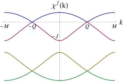
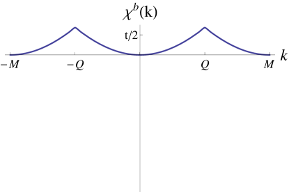
Figure 2: In this figure, we show the mean field band structure for the Spinons and Holons. On the left we show the lowest four bands (there are two flat bands at higher energy which are not shown in the figure). Of these four bands, at half-filling, the lowest three fill out thus leading to Dirac cones for the dispersion of the low energy spinons. On the right we show the lowest band for the holon which is unoccupied as there are no holons at half-filling.

Finally, the question of the holon chemical potential $\mu_{b}$ needs some attention. We assume that the holon chemical potential is chosen so that the doping $x=0$ and the bosons remain uncondensed at zero temperature. These assumptions appear quite valid for an ARPES experiment on Herbertsmithite so long as the density $x$ of induced holes created by photoemission remains small. It turns out, to achieve this at zero temperature, any negative value of $\mu_{b}$ will suffice. However, a specific value will be chosen at finite temperatures in the experimentally relevant regime. We will therefore leave $\mu_{b}$ as a finite negative valued parameter in our theory. This produces the spectrum for the holons on the right side of Fig. 2.

III.1 The Spectral Function

Let us now turn to the mean field predictions for the ARPES spectral function defined by

$$A(\vec{k},\omega)=\\ -\frac{1}{\pi}\text{Im}\left[\int d\vec{r}\int_{-\infty}^{0}dt\left\langle c_{\vec{r},\sigma}^{\dagger}(t)c_{\vec{0}}(0)\right\rangle e^{-i{\vec{r}}\cdot{\vec{k}}-i\omega t}\right].$$ (10)

At the mean field level, this becomes

$$A_{mean}(\vec{k};\omega)\propto\sum_{\lambda_{1},\lambda_{2}}\int dq\,\delta\left(\omega-2t\chi^{b}_{\lambda_{1}}\left(\vec{k}-\vec{q}\right)+J\chi^{f}_{\lambda_{2}}\left(\vec{q}\right)\right)$$ (11)

where $\chi^{b}$,$\chi^{f}$ are the holon and spinon bands respectively and $\lambda_{1}$, $\lambda_{2}$ are band indices. The above expression has a clear interpretation: all the possible spinon-holon combinations with the right energy-momentum values combine to give the requisite hole at wavevector $\vec{k}$ and energy $\omega$ in the ARPES experiment. The factor of two with the holon or $t$ term in the above equation comes from spin counting but we need not overly worry about such factors. Ultimately, we are concerned with the $\omega$ or $\vec{k}$ dependence of the spectral function, and the functional form of this dependence is not going to be affected by such factors of two.

We are interested in the low energy behavior of the system in general and the spectral function in particular. We can easily see for the mean-field bands, most of the bands won’t play any role in the low energy behavior. It is only the highest filled spinon band and the lowest empty holon band that will contribute to the $\omega\rightarrow 0$ limit. For these bands, the low $\omega$ contribution will come from near specific wavevectors that connects the “Dirac” points of spinon bands to the minima of the holon bands. Near these specific wavevectors, the spinon and holon spectrum are linear and quadratic in $|\vec{q}|$. Thus, for smaller and smaller $\omega$, the linear term starts dominating in the integral and we get $A_{mean}\propto\omega$ for $\omega\rightarrow 0$. We show in Fig. 3 a numerical confirmation of the mean-field result. In addition, a back-of-envelope estimate tell us that linearity is expected up to about $\frac{t^{2}}{4J}\frac{\chi^{\prime}(Q_{f})^{2}}{\chi^{\prime}(Q_{b})}$ where $Q_{f}$ and $Q_{b}$ are the momenta at which the Dirac point and the holon minimum sit respectively. This linear behavior in energy is—if the mean-field theory were qualitatively correct—a key signature easily extracted from ARPES data.

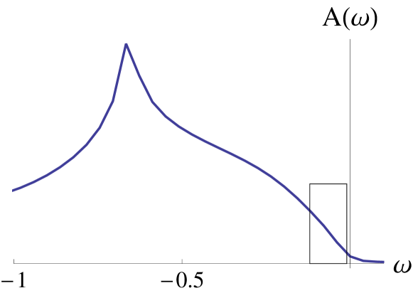
Figure 3: In this figure, we show a numerically calculated representative spectrum for ARPES at the mean-field level. The numerical calculation confirms the linear behavior at low energies (highlighted using the rectangle) as argued for in the text (Sec III). Our choice of parameters were $J=0.5$ and $t=1$.

III.2 Continuum limit and scaling analysis

To understand fluctuations around mean field theory, a continuum limit approximation is essential. To this end, it is useful to carry this out first directly at the mean field level. Such an analysis will thus facilitate the scaling discussion when we go beyond mean-field theory. We define the continuum fields through

$$b_{\vec{R},d} = \sum_{n}\phi_{n}(\vec{R})U^{n}_{d}e^{iQ_{b}^{n}.(\vec{R})}$$

$$f_{\vec{R},d,\sigma} = \sum_{m,\lambda}\psi_{m,\lambda,\sigma}(\vec{R})U^{m}_{\lambda,d}e^{iQ_{f}^{m}.(\vec{R})}$$ (12)

where $\vec{R}$ refers to unit-cell index and $d$ refers to the index of the bases within the unit-cell. The sum is understood to be restricted to the low-energy modes, $n$ refers to the index characterizing the (three) holon minima in the holon band structure and $Q_{b}^{n}$ are the momenta in the Brillouin zone where the minima sit respectively, $m$ refers to the index characterizing the (two) Dirac points in the spinon band structure and $Q_{f}^{n}$ are the momenta in the Brillouin zone where the Dirac points sit respectively, $\sigma$ is the spin index, and $\lambda$ is the “Dirac” index characterizing the branches of the Dirac cone. $U^{n}_{d}$ and $U^{m}_{\lambda,d}$ are the eigenmodes of the bandstructure corresponding to holon minima and Dirac points respectively.

Thus, using the definition of Eq. 10 we can get for the continuum spectral function

$$A(Q_{f}^{m}-Q_{b}^{n}+q,\omega)=\sum_{\lambda,\sigma}M^{mn}_{\lambda,\sigma}A^{m,n}_{\lambda,\sigma}(q,\omega)$$ (13)

where $M^{mn}_{\lambda,\sigma}$ are contributions due to the eigen modes $U^{n}_{d}$ and $U^{m}_{\lambda,\vec{d}}$. $M^{mn}_{\lambda,\sigma}$ is independent of momentum and energy, and $A^{m,n}_{\lambda,\sigma}(q,\omega)$ contains all the momentum and energy dependence which is what we will focus on in the following.

With the definitions in Eq. 12, the low energy physics (of the quadratized Hamiltonian Eq. 6) is described by an effective 2+1 continuum field theory where the spinons are described by a Dirac fermionic field (due to the linear spectrum near the spinon chemical potential) $\Psi$ - a linear combination of $\psi_{\lambda}$, details of which can be found in Appendix A of Ref. Hermele2, - and the holons are described by a non-relativistic complex scalar field $\phi$ (due to the quadratic spectrum near the holon chemical potential). The Lagrangian for this field theory is

$$L_{free}=\int drdt\bigg{[}\bar{\Psi}(r,t)\gamma^{\mu}\partial_{\mu}\Psi(r,t)+\\ \phi^{*}(r,t)(i\partial_{t}+\partial_{r}^{2}/2m_{holon}-\mu_{b})\phi(r,t)\bigg{]}$$ (14)

The mean field fixed point is then determined by how these fields scale when space-time is scaled (and from this field scalings, we can write a scaling form for the Spectral function). When we scale as $r\rightarrow br;t\rightarrow bt$, it can be shown that scaling the fields as $\Psi\rightarrow b^{-1}\Psi;\phi\rightarrow b^{-1}\phi$ leaves the Lagrangian invariant. Using these field and space-time scalings and the continuum limit of Eq. 10

$$A_{mean}(\vec{k},\omega)\propto\\ \text{Im}\int dr\int_{-\infty}^{0}dt\langle\phi(\vec{r},t)\bar{\Psi}(\vec{r},t)\Psi(\vec{0},0)\phi^{*}(\vec{0},0)\rangle e^{-i{\vec{r}}\cdot{\vec{k}}-i\omega t},$$ (15)

we can show that spectral function scales as $A_{mean}(b^{-1}\omega,b^{-1}k)=b^{-1}A_{mean}(\omega,k)$ which is consistent with $A_{mean}\propto\omega$ as we obtained from more elementary considerations.

IV Beyond Mean-field Theory

The $t$-$J$ Hamiltonian remains invariant under a local gauge transformation made to the spinons and holons

$$b_{i}\rightarrow e^{i\theta_{i}}b_{i},\quad f_{i,\sigma}\rightarrow e^{i\theta_{i}}f_{i,\sigma}.$$ (16)

Thus, when we include the fluctuations beyond the mean field level, the resulting continuum Lagrangian should remain invariant under this transformation. As is well know, this is achieved through replacing the derivative by a covariant derivative $\partial_{\mu}\rightarrow D_{\mu}=\partial_{\mu}-ieA_{\mu}$ where $e$ is the electric charge and $A_{\mu}$ is a Maxwell vector potential satisfying the usual transformation law: $A_{\mu}(\vec{r},t)\rightarrow A_{\mu}(\vec{r},t)-\partial_{\mu}\theta(\vec{r},t)$ when $\Psi(\vec{r},t)\rightarrow e^{i\theta(\vec{r},t)}\Psi(\vec{r},t)$ and $\phi(\vec{r},t)\rightarrow e^{i\theta(\vec{r},t)}\phi(\vec{r},t)$. Thus, the beyond mean-field Lagrangian for the spinons and holons is

$$L=\int drdt\bigg{[}\bar{\Psi}(r,t)\gamma^{\mu}D_{\mu}\Psi(r,t)-\frac{1}{4}F_{\mu\nu}F_{\mu\nu}\\ \phi^{*}(r,t)(iD_{t}+(D_{x}^{2}+D_{y}^{2})/2m-\mu)\phi(r,t)\bigg{]}$$ (17)

where $F_{\mu\nu}=\partial_{\mu}A_{\nu}-\partial_{\nu}A_{\mu}$.

Now, Dirac fermions coupled to an $U(1)$ gauge field in $2+1$ dimensions is a strongly-coupled problem. To make progress, the gauge field contributions are typically handled by a large-N perturbation series Appelquist ; KimLee ; RantnerWen ; Hermele0 ; Hermele1 ; Franz ; Kaveh arising from $N$ flavors of the Dirac fermions. In this case, for large $N$, $1/N$ provides a formal small parameter provided the coupling scales with $N$ as $e^{2}\sim 1/N$. When the pertubation theory is carried out, one finds that the spinon propagator acquires an anomalous dimension because of the gauge field coupling $e$ (See e.g. Ref. [Hermele1, ]’s Appendix B). Formally, when we scale space-time as $r\rightarrow br;t\rightarrow bt$, the Dirac field scales as $\Psi\rightarrow b^{-1-\delta}\Psi$ where $\delta$ is the anomalous dimension at the fixed point. This anomalous dimension is the manifestation of the fact that the gauge-field contributions make the theory flow to a new fixed point (with different scaling) away from the mean-field fixed point. The general intuition is that the strength of fluctuations will only increase when $N$ is decreased and thus this new fixed point (called Algebraic fixed point) may dominate a large portion of the low energy sector for the physical case of $N=4$.

Our aim is to understand the effect of the beyond mean-field fluctuations on the holons, a subject not visited in previous studies due mostly to a focus on the Heisenberg model. In an earlier workRantnerWen , the electron spectral function for the Dirac Spin Liquid was considered in the context of underdoped cuprates, but this study differs significantly from ours in that they assumed that the bosons were condensed as they were motivated by pseudogap phenomena at finite doping. To reiterate our main assumption, we will suppose that the bosons are uncondensed, i.e. $\mu<0$, an assumption that seems reasonable if a successful ARPES experiment is to be performed. In the ideal case at half-filling, under the exact single occupancy constraint, there are no bosons around. When an ARPES photon ejects an electron, a boson is created before it gets destroyed by the replenishing of the electron through an electronic bath connected to the sample. This boson is then uncondensed at the temperature of the experiment because they are very dilute. If the electrons fail to be replenished, however, the bosons density could grow to a level where they condense. The resulting charged surface, though, would then affect the trajectory of the ejected electron and the ARPES experiment would fail to obtain meaningful data. Hence, a successful ARPES experiment would probe the undoped insulator only when the bosons remain uncondensed.

In the following Section IV. A, we discuss in detail the effect of gauge field on the bosonic field. We find that the gauge-field renormalized bosonic propagator does not acquire an anomalous dimension unlike the spinon propagator and still scales as a free boson, $\phi\rightarrow b^{-1}\phi$ upon $r\rightarrow br;t\rightarrow bt$. This is expected due to the finite energy cost of the bosonic excitations when they remain uncondensed. Furthermore in Section IV B, we show that the electron propagator made of the spinon and boson also retains its mean-field scaling upon taking lowest order gauge-field corrections. This is intriguing when contrasted with the anomalous scaling of the spinon.

IV.1 Renormalized Perturbation Theory for Holons

Let us now focus on the holon part of the Lagrangian—a non-relativistic complex bosonic field—that couples only to the $U(1)$ gauge field:

$$\mathscr{L}_{\phi}=\int d^{2}rdt\phi^{*}_{0}(\vec{r},t)(iD_{t}+\frac{D^{2}_{x}+D^{2}_{y}}{2m_{b}}-\mu_{b})\phi(\vec{r},t)$$ (18)

where $D_{\mu}=\partial_{\mu}-ieA_{\mu}(\vec{r},t)/sqrt{N}$ as stated earlier though now extended to arbitrary $N$ , the bare mass parameter $m_{b}$ characterises the curvature of the quadratic dispersion at the bottom of the holon band and $\mu_{b}$ is the bare holon chemical potential. With the assumption of uncondensed holons, $\mu_{b}$ is strictly negative, i.e. less than the bottom of holon band.

To understand the holon propagator in the large-N limit, it turns out we need to first understand the photon propagator. The bare photon propagator receives a finite renormalization due to both spinon bubbles and holon bubbles even at leading order in $1/N$. However, the holon bubble does not affect the renormalization of the most singular contribution arising from the fermionic spinon vacuum bubble KimLee . Thus, the O(1/N) corrected photon propagator is (see Eqn B5 of Ref. [Hermele1, ])

$$\includegraphics[width=86.72267pt]{photonprop.eps}=\frac{16}{N|q|}(\delta_{\mu\nu}+(\xi-1)\frac{q_{\mu}q_{\nu}}{q^{2}})+\ldots$$ (19)

where the ellipsis represents subdominant corrections that are smaller than the term shown as $q\to 0$ and in the following we will use the Lorentz’s gauge, $\xi=1$. This Coulomb-like form is then the natural interaction that the holons feel.

For the perturbation theory we follow standard texts FieldTheory and define the original (bare) Lagrangian with bare parameters in terms of the physical parameters (to be determined by the experiment). We start by defining a renormalized bosonic field in terms of the bare field

$$\phi_{0}\equiv Z^{1/2}\phi\cdots Z\equiv\text{field rescaling of bosons}$$ (20)

Putting this in to Eqn. 18, the Lagrangian looks like

$$\mathscr{L}_{\phi}=\int d^{2}rdt\bigg{[}\phi^{*}(\vec{r},t)(iD_{t}+\frac{D^{2}_{x}+D^{2}_{y}}{2m}-\mu)\phi(\vec{r},t)\\ +\phi^{*}(\vec{r},t)\frac{D^{2}_{x}+D^{2}_{y}}{2\delta_{m}})\phi(\vec{r},t)\\ +\delta_{Z}\phi^{*}(\vec{r},t)iD_{t}\phi(\vec{r},t)+\delta_{\mu}\phi^{*}(\vec{r},t)\phi(\vec{r},t)\bigg{]}$$ (21)

where $\delta_{Z}=Z-1$, $\delta_{m}=\left(\frac{1}{m}-\frac{Z}{m_{b}}\right)^{-1}$ and $\delta_{\mu}=-Z\mu_{b}+\mu$ with $\mu$ a renormalized version of $\mu_{b}$ not to be confused with the chemical potential of the electrons. These are the counterterms. Since the holons do not renormalize the photon field, it’s propagator stays the same as in Eqn. 19.

We rewrite the renormalized Lagrangian as a free part

$$\mathscr{L}^{r}_{free}=\int d^{2}rdt\phi^{*}(\vec{r},t)(i\partial_{t}+\frac{\partial^{2}_{x}+\partial^{2}_{y}}{2m}-\mu)\phi(\vec{r},t)$$ (22)

a counter term part

$$\mathscr{L}_{counter}=\int d^{2}rdt\bigg{[}\delta_{z}\phi^{*}(\vec{r},t)i\partial_{t}\phi(\vec{r},t)+\\ \phi^{*}(\vec{r},t)\frac{\partial^{2}_{x}+\partial^{2}_{y}}{2\delta_{m}}\phi(\vec{r},t)+\delta_{\mu}\phi^{*}(\vec{r},t)\phi(\vec{r},t)\bigg{]}$$ (23)

and an interaction part

$$\mathscr{L}_{int}=\int d^{2}rdt\bigg{[}Z\phi^{*}(\vec{r},t)A_{t}(\vec{r},t)\phi(\vec{r},t)\\ -iZ\phi^{*}(\vec{r},t)\left(\frac{\partial_{x}A_{x}(\vec{r},t)+\partial_{y}A_{y}(\vec{r},t)}{m_{b}}\right)\phi(\vec{r},t)\\ +\phi^{*}(\vec{r},t)\left(-Z\frac{A^{2}_{x}(\vec{r},t)+A^{2}_{y}(\vec{r},t)}{2m_{b}}\right)\phi(\vec{r},t)\bigg{]}$$ (24)

Therefore, the Feynman rules are given by: the boson propagator line

$$\includegraphics[width=86.72267pt]{Bosonprop.eps}=\frac{1}{\omega-\big{(}|\vec{k}|^{2}/2m+|\mu|\big{)}+i\epsilon}$$ (25)

the counter terms by

$$\includegraphics[width=86.72267pt]{Zvertex.eps}=\delta_{Z}\omega$$

$$\includegraphics[width=86.72267pt]{Mcounterterm.eps}=|\vec{k}|^{2}/2\delta_{m}$$

$$\includegraphics[width=86.72267pt]{mucounterterm.eps}=\delta_{\mu}$$ (26)

and the interaction vertices by

• Boson-Gauge Field’s “Time” component vertex

  $$\includegraphics[width=86.72267pt]{Bosontimevertex.eps}=Z$$ (27)

• Boson-Gauge Field’s “Space” component vertices

  $$\includegraphics[width=86.72267pt]{Bosonspacevertex.eps}=Zk_{i}/m_{b}$$ (28)

  where $i$ refers to the Gauge field’s “space” component we are looking, i.e. if $\phi$ interacts with $A_{x}$, then the vertex will contribute $k_{x}$, etc. The are actually two such vertices of this type, one where $k_{i}$ goes with the incoming boson’s ($\phi$) momentum and one where $k_{i}$ goes the outgoing boson’s ($\phi^{*}$) momentum. We can collected all these vertices together by defining $V^{\mu}(\vec{k})$ to be Eq. (27) for $\mu=t$ and Eq. (28) for $\mu=x$ or $\mu=y$.

• Boson-Gauge Field’s quartic vertex

  $$\includegraphics[width=86.72267pt]{Bosonspacevertex2.eps}=-Z/2m_{b}$$ (29)

Note: energy-momentum is conserved at the interaction vertices.

Now, we look at the 2-point free vertex function $\Gamma_{0}^{2}(\vec{k},\omega)=\omega-\big{(}|\vec{k}|^{2}/2m+|\mu|\big{)}$ and impose our renormalization conditions on the renormalized 2-point function

$$\Gamma^{2}(\vec{k}=(0,0),\omega=M) = \mu=-|\mu|$$

$$d\Gamma^{2}/d\omega(\vec{k}=(0,0),\omega=M) = 1$$

$$d\Gamma^{2}/dk^{2}(\vec{k}=(0,0),\omega=M) = -1/2m$$ (30)

In other words, we chose the time-like scale $(\vec{k},\omega)=((0,0),M)$ as the renormalization scale.

With the above setup, let us now turn to our main interest, the holon’s anomalous dimension which is governed by the holon field rescaling $Z$ FieldTheory . We will consider this to order $1/N$ through the diagrams of the propagator shown in Fig. 4. If we view the self energy as the contribution to $\Gamma^{2}$ of $\Gamma^{2}(\vec{k},\omega)=\Gamma_{0}^{2}(\vec{k},\omega)-\Sigma(\vec{k},\omega)+\text{counter terms}$, then from the diagrams in the figure, we see that the second renormalization condition becomes

$$\therefore\frac{d\Gamma^{2}}{d\omega}=1\Rightarrow\frac{d\Sigma}{d\omega}{((0,0),M)}+\delta_{Z}=0$$ (31)

So, to understand $Z$ we need only consider $d\Sigma/d\omega$. Since the contributions of the last two counterterm diagrams and the diagram with the “$q=0$” bubble in Fig. 4 are independent of $\omega$, these terms are then unimportant here. Hence we obtain

$$\frac{d\Sigma(\vec{k},\omega)}{d\omega}=\frac{d}{d\omega}\int\frac{d^{2}qdq_{0}}{(2\pi)^{3}}\frac{16}{N|q|}$$ (32)

$$\times\frac{1+\frac{Z^{2}}{m^{2}_{b}}(2k_{x}-q_{x})^{2}+\frac{Z^{2}}{m^{2}_{b}}(2k_{y}-q_{y})^{2}}{\big{[}(\omega-q_{0})-((\vec{k}-\vec{q})^{2}/2m+|\mu|)+i\epsilon)\big{]}}$$

Taking the derivative, we then obtain

$$\frac{d\Sigma}{d\omega}{((0,0),M)}=-\frac{16}{N}\int\frac{d^{3}q}{(2\pi)^{3}}\frac{1}{|q|}$$ (33)

$$\times\frac{1+\frac{Z^{2}}{m^{2}_{b}}(q_{x})^{2}+\frac{Z^{2}}{m^{2}_{b}}(q_{y})^{2}}{\big{[}q_{0}-i\epsilon-M+|\vec{q}|^{2}/2m+|\mu|))\big{]}^{2}}$$

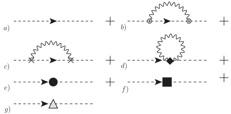
Figure 4: Perturbation Series for Bosons to first order in $O[1/N]$

To understand this integral, we need the following identity, whose origin lies in the branch cut singularity:

$$\lim_{\epsilon\to 0}\int^{\infty}_{-\infty}\frac{dx}{(x-(a+i\epsilon)))^{n}\sqrt{x^{2}+b^{2}}}$$ (34)

$$=2\int^{\infty}_{0}\frac{dy}{(i(b+y)-a)^{n}\sqrt{y^{2}+2by}},\quad b>0$$

Using this, we then obtain

$$\frac{d\Sigma}{d\omega}{((0,0),M)}=A\int^{\infty}_{-\infty}dq_{x}dq_{y}\int^{\infty}_{0}dy$$ (35)

$$\times\frac{1+\frac{Z^{2}}{m^{2}_{b}}(q_{x})^{2}+\frac{Z^{2}}{m^{2}_{b}}(q_{y})^{2}}{(i(y+|\vec{q}|)-M+|\vec{q}|^{2}/2m+|\mu|)^{2}}$$

$$\times\frac{1}{\sqrt{y^{2}+2|\vec{q}|y}}$$

Finally, to understand the behavior of the above integral in the infra-red, we introduce an UV cut-off $\Lambda$ for the integral and express everything with the scale of energy in units of this UV cut-off $\Lambda$.

$$\tilde{q}_{i}=\frac{q_{i}}{\Lambda},\tilde{y}=\frac{y}{\Lambda},\tilde{M}=\frac{M}{\Lambda},|\tilde{\mu}|=\frac{|\mu|}{\Lambda},\tilde{m}=\frac{m}{\Lambda}.$$ (36)

In terms of these rescaled variables, we then obtain

$$\frac{d\Sigma}{d\omega}{((0,0),\tilde{M})}=A\int^{1}_{-1}d\tilde{q}_{x}d\tilde{q}_{y}\int^{1}_{0}d\tilde{y}$$ (37)

$$\times\frac{1+\frac{Z^{2}}{m^{2}_{b}}(\tilde{q}_{x})^{2}+\frac{Z^{2}}{m^{2}_{b}}(\tilde{q}_{y})^{2}}{(i(\tilde{y}+|\vec{\tilde{q}}|)-\tilde{M}+|\vec{\tilde{q}}|^{2}/2\tilde{m}+|\tilde{\mu}|)^{2}}$$

$$\times\frac{1}{\sqrt{\tilde{y}^{2}+2|\vec{\tilde{q}}|\tilde{y}}}$$

Consider the infra-red limit $\lim\tilde{M}\rightarrow 0$, i.e. when the renormalization scale is in the infra-red. The self-energy integral simplifies to

$$\frac{d\Sigma}{d\omega}{((0,0),\tilde{M})}=A\int^{1}_{-1}d\tilde{q}_{x}d\tilde{q}_{y}\int^{1}_{0}d\tilde{y}$$ (38)

$$\times\frac{1+\frac{Z^{2}}{m^{2}_{b}}|\vec{\tilde{q}}|^{2}}{(i(\tilde{y}+|\vec{\tilde{q}}|)+|\vec{\tilde{q}}|^{2}/2\tilde{m}+|\tilde{\mu}|)^{2}}$$

$$\times\frac{1}{\sqrt{\tilde{y}^{2}+2|\vec{\tilde{q}}|\tilde{y}}}$$

The only singularity in the integrand comes from $\tilde{y}\rightarrow 0$, $|\vec{\tilde{q}}|\rightarrow 0$ because of $\sqrt{\tilde{y}^{2}+2|\vec{\tilde{q}}|\tilde{y}}$. The presence of $|\tilde{\mu}|$ automatically regulates the other denominator. Let’s say we do the $\tilde{y}$ integration first. Since, $\tilde{y}$ will dominate over $\tilde{y}^{2}$ when $\tilde{y}\rightarrow 0$, therefore $\sqrt{\tilde{y}^{2}+2|\vec{\tilde{q}}|\tilde{y}}\approx\sqrt{2|\vec{\tilde{q}}|\tilde{y}}$. As an integral over $\tilde{y}$, this is an integrable singularity. Similarly as an integral over (radial) $|\vec{\tilde{q}}|$, the $\sqrt{2|\vec{\tilde{q}}|\tilde{y}}$ is an integrable singularity.

Thus, in the infra-red limit $\tilde{M}\rightarrow 0$, $d\Sigma/d\omega$ is finite and hence can’t have a logarithmic contribution($\log{\tilde{M}}=\log{M/\Lambda}$). Through similar arguments, we can show that $\Sigma(\omega)$ is finite too. Also, the integral coming from the third renormalization condition in Eqn. 30 which determined $\delta_{m}$ will be finite as well. We mention this because in integral for $d\Sigma/d\omega$, we have the term $Z^{2}/m^{2}_{b}$ in the numerator and $m_{b}$ depends on $m$ and $\delta_{m}$. But the finiteness of ‘$\delta_{m}$’ integral guarantees us that there wouldn’t be any logarithmic contribution to $d\Sigma/d\omega$ because of the presence of the $Z^{2}/m^{2}_{b}$ term. Thus, our earlier conclusion - that $d\Sigma/d\omega$ has no logarithmic divergence - remains valid. In absence of logarithmic divergences the bosonic field won’t acquire an anomalous dimension FieldTheory , and thus $Z=1$.

IV.2 Large-N perturbative calculations for an electron

In the previous section we showed that large-N corrections to the holons are finite and thus the $1/N$ holon propagator is just a renormalized form of the mean-field holon propagator. As has been shown before by others, the $1/N$ spinon propagator does get a logarithmic correction. In this section, we work out the consequences of these two statements on to the electron propagator made of the a holon and a spinon that would be measured in an ARPES experiment.

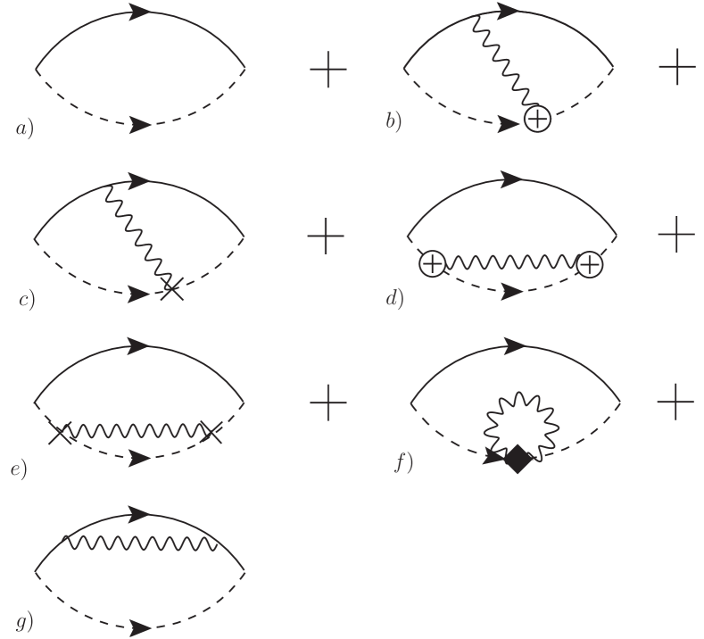
Figure 5: The terms in the perturbation series for the Hole propagator up to $O[1/N]$

The Feynman diagrams for the electron propagator to $O[1/N]$ are shown in Fig. 5. We are interested in finding out if the hole propagrator recieves any logarithmic corrections due to the gauge fluctuations due to divergent diagrams. Let us first look at Fig. 5 a) which is the continuum limit of the mean-field electron propagator $A_{mean}(\vec{q},\omega)$ studied in Sec. III and shown to be linear in $\omega$ through an analysis of mean-field band structure of spinons and holons and through a mean-field scaling argument. For our low-energy continuum theory (we use the same conventions for the spinon propagators as in Ref. Hermele1, ), this diagram is equal to

$${\bf A}_{a}(\vec{q},\omega)=\int d\omega_{1}d\vec{q}_{1}{\bf S}(\vec{q}_{1},\omega_{1})G(\vec{q}-\vec{q}_{1},\omega-\omega_{1})$$ (39)

where ${\bf A}_{a}$ is matrix spectral function that enters Eq. 13 and is related to the measured spectral function through matrix elements,

$${\bf S}(\vec{q},\omega)=\frac{1}{\gamma^{0}(\omega+i\epsilon sgn(\omega))+\vec{\gamma}\cdot\vec{q}}$$ (40)

and

$$G(\vec{q},\omega)=\frac{1}{(\omega-\omega_{1})+i\epsilon-\frac{|\vec{q}-\vec{q}_{1}|^{2}}{2m_{b}}-|\mu_{b}|}$$ (41)

is the boson propagator entering Eq. (25). Evaluating the frequency integral we arrive at

$${\bf A}_{a}(\vec{q},\omega)=\pi\int d\vec{q}_{1}\frac{i\gamma^{0}-\vec{\gamma}\cdot\hat{q}_{1}}{\omega+i|\vec{q}_{1}|-\frac{|\vec{q}-\vec{q}_{1}|^{2}}{2m_{b}}-|\mu_{b}|}$$ (42)

In the infrared limit at the Dirac point $\omega\rightarrow 0$, $\vec{q}=(0,0)$, the integrand in Eq. 42 has a finite denominator, thus there is no divergence. This is as we would have expected of the mean-field hole propagator and the leading term (in $\omega$) of the (finite) integral is linear in $\omega$ (as concluded from other arguments in Sec III). Since in the previous subsection we showed that the holon recieves only finite corrections at $1/N$, the diagrams Fig. 5 d), e) and f) are also finite as can be shown in a similar manner as the evaluation of the mean-field diagram above. Hence, diagrams a), d), e) and f) are all finite diagrams as far as divergences are considered and are consistent with the mean field scaling.

We proceed to look at the diagram Fig. 5 b) and c) where a photon is exchanged between the holon and the spinon. This diagram equals to

$${\bf A_{b}}(\vec{q},\omega)=\!\!\int d\omega_{1}d\vec{q}_{1}d\omega_{2}d\vec{q}_{2}\bigg{[}\\ {\bf S}(\vec{q}_{1},\omega_{1}){\bf S}(\vec{q}_{1}-\vec{q}_{2},\omega_{1}-\omega_{2})\\ \times G(\vec{q}-\vec{q}_{1},\omega-\omega_{1})G(\vec{q}-\vec{q}_{1}+\vec{q}_{2},\omega-\omega_{1}+\omega_{2})\\ \gamma^{\mu}D_{\mu\nu}(\omega_{2},\vec{q}_{2})[V^{\nu}(\vec{q}-\vec{q}_{1})+V^{\nu}(\vec{q}-\vec{q}_{1}+\vec{q}_{2})]\bigg{]}$$ (43)

where $D_{\mu\nu}(\vec{q},\omega)$ is the photon propagator of Eq. (19) and $V^{\mu}(\vec{k})$ is defined in Eqs. (27) and (28). Doing the $\omega_{1}$-integral as a contour integral by closing on lower-half plane we arrive at

$$=\frac{16\pi}{N}\int d\vec{q}_{1}d\omega_{2}d\vec{q}_{2}\bigg{[}\frac{i\gamma^{0}-\vec{\gamma}\cdot\hat{q}_{1}}{\omega+i|\vec{q}_{1}|-\frac{|\vec{q}-\vec{q}_{1}|^{2}}{2m}-|\mu|}\\ \times\frac{\gamma^{0}(-i|\vec{q}_{1}|-\omega_{2})+\vec{\gamma}\cdot(\vec{q}_{1}-\vec{q}_{2})}{(\omega+i|\vec{q}_{1}|+\omega_{2})+i\epsilon-\frac{|\vec{q}-\vec{q}_{1}+\vec{q}_{2}|^{2}}{2m}-|\mu|}\\ \times\frac{\gamma^{\mu}[V^{\mu}(\vec{q}-\vec{q}_{1})+V^{\mu}(\vec{q}-\vec{q}_{1}+\vec{q}_{2})]}{\sqrt{\omega^{2}_{2}+|\vec{q}_{2}|^{2}}}\bigg{]}$$ (44)

and using Eq. IV.1 to do the $\omega_{2}$ integral this further reduces to

$$=\frac{32\pi}{N}\int d\vec{q}_{1}d\vec{q}_{2}\bigg{[}\frac{i\gamma^{0}-\vec{\gamma}\cdot\hat{q}_{1}}{\omega+i|\vec{q}_{1}|-\frac{|\vec{q}-\vec{q}_{1}|^{2}}{2m}-|\mu|}\\ \times\int^{\Lambda}_{0}dy\frac{\gamma^{0}(-i|\vec{q}_{1}|-i(|\vec{q}_{2}|+y))+\vec{\gamma}\cdot(\vec{q}_{1}-\vec{q}_{2})}{(\omega+i|\vec{q}_{1}|+i(|\vec{q}_{2}|+y))-\frac{|\vec{q}-\vec{q}_{1}+\vec{q}_{2}|^{2}}{2m}-|\mu|}\\ \times\gamma^{\mu}[V^{\mu}(\vec{q}-\vec{q}_{1})+V^{\mu}(\vec{q}-\vec{q}_{1}+\vec{q}_{2})]\frac{1}{\sqrt{y^{2}+2y|\vec{q}_{2}|}}\bigg{]}$$ (45)

Looking at $\omega\rightarrow 0$, $\vec{q}=(0,0)$ again (the infrared limit at the Dirac point), we see that the only singular piece in the integrand is $\frac{1}{\sqrt{y^{2}+2y|\vec{q}_{2}|}}$ which (as argued in Sec III b) is an integrable singularity. Thus, the diagrams Fig. 5 b) and c) give only finite corrections to the hole propagator.

We finally come to the diagram Fig. 5 g), where the loop on the spinon propagator has been shown to give a logarithmic correction to the spinon propagator. We want to know what is the effect of this logarithmic correction on the electron propagator. This diagram equals

$$= \frac{8}{3\pi^{2}N}\int d\omega_{1}d\vec{q}_{1}\left[\frac{(\gamma^{0}\omega_{1}+\vec{\gamma}\cdot\vec{q}_{1})\log(\sqrt{\omega^{2}_{1}+|\vec{q}_{1}|^{2}}/\Lambda)}{\omega^{2}_{1}+|\vec{q}_{1}|^{2}}\right]\left[\frac{1}{(\omega-\omega_{1})+i\epsilon-\frac{|\vec{q}-\vec{q}_{1}|^{2}}{2m}-|\mu|}\right]$$ (46)

where the logarithm is due to photon-spinon loop (see Eq. C9 of Ref. Hermele1, ). We can express $\log(\sqrt{\omega^{2}_{1}+|\vec{q}_{1}|^{2}}/\Lambda)$ as $(1/2)(\log((\omega_{1}+i\vec{q}_{1}/\Lambda)+\log((\omega_{1}-i\vec{q}_{1})/\Lambda))$. As a function of (complex) $\omega_{1}$, we show the branch cut structure due to the logarithms in Fig. 6. Thus we will do the $\omega_{1}$ integral as a contour integral keeping in mind that for the $\log((\omega_{1}+i\vec{q}_{1}/\Lambda)$ term, we close the contour on the upper-half plane, while for $\log((\omega_{1}-i\vec{q}_{1}/\Lambda)$, we close the contour on the lower-half plane. By capturing residues we get that the diagram equals

$$= A+B+C\text{ ... where}$$

$$A = \frac{4}{3\pi N}\int d\vec{q}_{1}\frac{(-i\gamma^{0}+\vec{\gamma}\cdot\hat{q}_{1})\log(-\frac{2i|\vec{q}_{1}|}{\Lambda})}{\omega+i|\vec{q}_{1}|-\frac{|\vec{q}-\vec{q}_{1}|^{2}}{2m}-|\mu|}$$

$$B = \frac{4}{3\pi N}\int d\vec{q}_{1}\frac{(i\gamma^{0}+\vec{\gamma}\cdot\hat{q}_{1})\log(\frac{2i|\vec{q}_{1}|}{\Lambda})}{\omega-i|\vec{q}_{1}|-\frac{|\vec{q}-\vec{q}_{1}|^{2}}{2m}-|\mu|}$$

$$C = -\frac{8i}{3\pi N}\int d\vec{q}_{1}\frac{(\gamma^{0}(\omega-\frac{|\vec{q}-\vec{q}_{1}|^{2}}{2m}-|\mu|)+\vec{\gamma}\cdot\vec{q}_{1})}{(\omega-\frac{|\vec{q}-\vec{q}_{1}|^{2}}{2m}-|\mu|)^{2}+|\vec{q}_{1}|^{2}}$$ (47)

$$\times\log(\frac{\omega+i|\vec{q}_{1}|-\frac{|\vec{q}-\vec{q}_{1}|^{2}}{2m}-|\mu|}{\Lambda})$$

In the infrared limit at the Dirac point (i.e. $\omega\rightarrow 0$, $\vec{q}=(0,0)$), the above simplifies to

$$= A+B+C\text{ ... where}$$

$$A = \frac{4}{3\pi N}\int d\vec{q}_{1}\frac{(-i\gamma^{0}+\vec{\gamma}\cdot\hat{q}_{1})(\log(\frac{2|\vec{q}_{1}|}{\Lambda})-\frac{i\pi}{2})}{\omega+i|\vec{q}_{1}|-\frac{|\vec{q}_{1}|^{2}}{2m}-|\mu|}$$

$$B = \frac{4}{3\pi N}\int d\vec{q}_{1}\frac{(i\gamma^{0}+\vec{\gamma}\cdot\hat{q}_{1})(\log(\frac{2|\vec{q}_{1}|}{\Lambda})+\frac{i\pi}{2})}{\omega-i|\vec{q}_{1}|-\frac{|\vec{q}_{1}|^{2}}{2m}-|\mu|}$$

$$C = -\frac{8i}{3\pi N}\int d\vec{q}_{1}\frac{(\gamma^{0}(\omega-\frac{|\vec{q}_{1}|^{2}}{2m}-|\mu|)+\vec{\gamma}\cdot\vec{q}_{1})}{(\omega-\frac{|\vec{q}_{1}|^{2}}{2m}-|\mu|)^{2}+|\vec{q}_{1}|^{2}}$$ (48)

$$\times\log(\frac{\omega+i|\vec{q}_{1}|-\frac{|\vec{q}_{1}|^{2}}{2m}-|\mu|}{\Lambda})$$

The $\vec{\gamma}\cdot\hat{q}_{1}$ and $\vec{\gamma}\cdot\vec{q}_{1}$ terms are odd under inversion and hence upon integration equal zero. $A+B$ is finite. This can be seen by expanding the denominators of $A$ and $B$ in $|\vec{q}_{1}|$. At lowest order for $|\vec{q}_{1}|$, the two (singular) logarithmic contributions cancel each other out. Higher orders in $|\vec{q}_{1}|$ don’t have singular integrands as $|\vec{q}_{1}|^{n}\log(|\vec{q}_{1}|)\rightarrow 0$ as $|\vec{q}_{1}|\rightarrow 0$ for $n\geq 1$.

We can write the logarithm in $C$ as $\log(\frac{\sqrt{(\omega-\frac{|\vec{q}_{1}|^{2}}{2m}-|\mu|)^{2}+|\vec{q}_{1}|^{2}}}{\Lambda})+i\arctan(\frac{|\vec{q}_{1}|}{\omega-\frac{|\vec{q}_{1}|^{2}}{2m}-|\mu|})$. We focus on the imaginary part of $C$ since it is the most singular part. We can write this as

$$\Im[C] = -\frac{4}{3\pi N}\int d\vec{q}_{1}\frac{\gamma^{0}(\omega-\frac{|\vec{q}_{1}|^{2}}{2m}-|\mu|)}{(\omega-\frac{|\vec{q}_{1}|^{2}}{2m}-|\mu|)^{2}+|\vec{q}_{1}|^{2}}$$

$$\times\log(\frac{(\omega-\frac{|\vec{q}_{1}|^{2}}{2m}-|\mu|)^{2}+|\vec{q}_{1}|^{2}}{\Lambda^{2}})$$

$$= -\frac{8}{3N}\int^{\Lambda}_{0}mdy\frac{\gamma^{0}(\omega-|\mu|-y)\log(\frac{(\omega-|\mu|-y)^{2}+2my}{\Lambda^{2}})}{(\omega-|\mu|-y)^{2}+2my}$$

and we see that the integrand is finite everywhere on the integration domain (with the UV cut-off). Therefore the integral cannot have any singular/logarithmic term. Thus we conclude that $O[1/N]$ corrections to the hole propagator due to the gauge fluctuations are finite. Therefore the $O[1/N]$ scaling of the ARPES spectral function is the same as the mean-field scaling.

\psfrag{Imom}{$\Im[\omega_{1}]$}\psfrag{Reom}{$\Re[\omega_{1}]$}\psfrag{iq}{$i|\vec{q}_{1}|$}\psfrag{miq}{$-i|\vec{q}_{1}|$}\includegraphics[width=411.93767pt]{Branchcut.eps}

Figure 6: We show the branch cuts in a) of $\log(\frac{\omega_{1}+i|\vec{q}_{1}|}{\Lambda})$ and in b)

of $\log(\frac{\omega_{1}-i|\vec{q}_{1}|}{\Lambda})$

V Discussion

The key prediction of our work is that the ARPES spectral function for the putative spin liquid, Herbertsmithite, will show a linear low-energy behavior if the ground state has Dirac Spinons. This prediction is expected to be unique to the Dirac Spin Liquid as the Dirac point-like Fermi “surface” is not generic. Thus, other spin liquid ground states might generically be expected to have different energy dependences. Recently, NMR experiments LeeSingleCrystal1 were performed on single crystal Herbersmithite and the authors reported that their results are not in contradiction with a DSL. This makes the case for an ARPES experiment on Herbertsmithite even more exciting since, as stressed before, our prediction is a falsifiable prediction.

Another unique feature of our prediction is based on the fact that DSL is a high symmetry state in momentum space. Thus, the linear energy dependence will be most clearly observable at very specific momenta (i.e., momenta that connect these high symmetry points in the Brillouin Zone coming from the Dirac points for spinons and the dispersion minima for the holons $Q^{m}_{f}-Q^{n}_{b}$)). Observation of these momenta would be another strong evidence for a DSL.

We found that the holons in the Dirac spin liquid get trivial renormalizations from the gauge field fluctuations and remain as free bosons. On the other hand, as has been shown in earlier literature, the Dirac spinons do get nontrivial logarithmic renormalization from the gauge field fluctuations. This feature points to a dramatic spin-charge separation in the Dirac spin liquid.

In this paper, we have discussed how ARPES can provide an avenue to prove the existence of spinons in Kagome Antiferromagnet. Existence of spinons would raise two obvious questions : 1) How would one detect the corresponding charged holons ?, and 2) How would one detect the photons corresponding to the U(1) gauge field ?

Detection of holons can be envisaged perhaps through a transport experiment. Since the holons are charged bosons, we can expect to probe their existence in transport measurements. Since the low energy holons occur at particular non-zero momenta in the zone, there might be a non-trivial angular dependence of conductance in a sample which can be compared against theoretical predictions. Detection of the “photon” is probably a harder task. These photons will of course contribute to the specific heat along with spinons and one will have to separate the two contributions. Thermal conductivity measurements can similarly get contributions from the photons.

In conclusion, frustrated quantum magnets offer an universe of interesting objects including the one we focused on in this study : Dirac spinons, U(1) photons and non-interacting bosons built out of a Dirac spin liquid state. Herbertsmithite provides with an ideal candidate material to explore this universe and find these exotic objects. Finding the Spinon in Nature will certainly be a big step in the uncovering of that universe and a successful ARPES experiment on Herbertsmithite might go a long way in this regard.

Acknowledgements. We thank Kyle Shen, Chris Henley and Siddharth Parmeswaran for useful discussions. During the work, SP was supported by NSF grant DMR 1005466.

References

- (1) B. S. Shastry and B. Sutherland, Phys. Rev. Lett. 47, 964 (1981); L. D. Faddeev and L. A. Takhtajan, Phys. Lett. 85A, 375 (1981).
- (2) C. Mudry and E. Fradkin, Phys. Rev. B 49, 5200 (1994).
- (3) Kim, B. J., H. Koh, E. Rotenberg, S.-J. Oh, H. Eisaki, N. Motoyama, S. Uchida, et al. 2006, Nature Physics 2 (6) (May 21): 397-401.
- (4) Andrea Damascelli, Zahid Hussain, and Zhi-Xun Shen, Rev. Mod. Phys. 75, 473 (2003).
- (5) M.P. Shores et al., J. Am. Chem. Soc. 127, 13462 (2005).
- (6) J.S. Helton et al., Phys. Rev. Lett. 98, 107204 (2007).
- (7) M.A. de Vries et al., Phys. Rev. Lett. 100, 157205 (2008).
- (8) J.S. Helton et al., Phys. Rev. Lett. 104, 147201 (2010).
- (9) Experimental signatures of spin-liquid physics on the kagome lattice, Talk by Y.S. Lee at International Conference on Highly Frustrated Magnetism 2012, Hamilton, Ontario, Canada.
- (10) Wulferding D, Lemmens P, Scheib P, Roder J, Mendels P, Chu S, Han T and Lee Y S, Phys. Rev. B 82, 144412 (2010).
- (11) Oren Ofer, Amit Keren, Jess H Brewer, Tianheng H Han and Young S Lee, J. Phys. Condens. Matter 23, 164207 (2011).
- (12) S. Yan, D. A. Huse, S. R. White, Science 332, 1173 (2011); S. Depenbrock, I. P. McCulloch, and U. Schollwöck, Phys. Rev. Lett. 109, 067201 (2012).
- (13) O. Cépas, C. M. Fong, P. W. Leung and C. Lhuillier, Phys. Rev. B 78, 140405(R) (2008)
- (14) M. B. Hastings, Phys. Rev. B 63, 14413 (2000)
- (15) Ying Ran, Michael Hermele, Patrick A. Lee, and Xiao-Gang Wen, Phys. Rev. Lett. 98, 117205 (2007).
- (16) Yasir Iqbal, Federico Becca, Sandro Sorella, Didier Poilblanc, arXiv:1209.1858 [cond-mat.str-el].
- (17) W. Rantner and X.-G. Wen, Phys. Rev. Lett. 86, 3871 (2001); W. Rantner and X.-G. Wen, Phys. Rev. B 66, 144501(2002).
- (18) Evelyn Tang, MPA fisher, Patrick Lee, arXiv:1210.0921.
- (19) Barnes, S. E., J. Phys. F: Met. Phys. 6, 1375 (1976).
- (20) Coleman, P., Phys. Rev. B 29, 3035 (1984).
- (21) M. Peskin and D. Schroeder, An Introduction to Quantum Field Theory, Addison-Wesley (1995) ; J. Zinn-Justin, Quantum Field Theory and Critical Phenomena, Clarendon Press (2002).
- (22) M. Hermele, Y. Ran, P. A. Lee and X-G Wen, Phys. Rev. B 77, 224413 (2008).
- (23) T. W. Appelquist, M. Bowick, D. Karabali, and L. C. R. Wijewardhana, Phys. Rev. D 33, 3704 (1986).
- (24) D. H. Kim and P. A. Lee, Ann. Phys.(N.Y) 272, 130 (1999).
- (25) M. Hermele, T. Senthil, M. P. A. Fisher, P. A. Lee, N. Nagaosa, and X.-G. Wen, Phys. Rev. B 70, 214437 (2004).
- (26) Michael Hermele, T. Senthil and Matthew P. A. Fisher, Phys. Rev. B 72, 104404 (2005).
- (27) M. Franz and Z. Tesanovic, Phys. Rev. Lett. 87, 257003 (2001); M. Franz, Z. Tesanovic and O. Vafek, Phys. Rev. B 66, 054535 (2002).
- (28) K. Kaveh and I. F. Herbut, Phys. Rev. B 71, 184519 (2005).
- (29) Here we are supressing the in otherwise , keeping in mind that ensures a perturbation series for the holon with as the small parameter as is usual in large N expansions.