Hadronic Models for LAT Prompt Emission Observed in Fermi Gamma-Ray Bursts

Abstract

This paper examines the possibility that hadronic processes produce the $\ga$100 MeV photons in the prompt phase of gamma-ray bursts (GRBs) observed by the Fermi-LAT. We calculate analytically the radiation from protons and from secondary electron-positron pairs produced by high energy protons interacting with gamma-rays inside of the GRB jet. We consider both photo-pion and Bethe-Heitler pair production processes to create secondary electrons and positrons that then radiate via inverse Compton and synchrotron processes. We also consider synchrotron radiation from the protons themselves. We calculate the necessary energy in protons to produce typical Fermi-LAT fluxes of a few $\mu$Jy at 100 MeV. For both of the photo-pion and Bethe-Heitler processes, we find that the required energy in protons is larger than the observed gamma-ray energy by a factor of a thousand or more. For proton synchrotron, the protons have a minimum Lorentz factor $\sim 2\times 10^{6}$. This is much larger than expected if the protons are accelerated by relativistic collisionless shocks in GRBs. We also provide estimates of neutrino fluxes expected from photo-hadronic processes. Although the flux from a single burst is below IceCube detection limits, it may be possible to rule out photo-hadronic models by adding up the contribution of several bursts. Therefore, photo-hadronic processes seem an unlikely candidate for producing the Fermi-LAT radiation during the prompt phase of GRBs.

1 Introduction

The Fermi satellite has detected 29 gamma-ray bursts (GRBs) with photons of energies $\ga$100 MeV with the Large Area Telescope (LAT) (Atwood et al., 2009). The photons detected during the prompt phase of GRBs by the Fermi-LAT are emitted with a delay of a few seconds for long GRBs, and are observed for a longer duration of time compared to the lower-energy photons ($\sim$1 MeV) observed by the Fermi Gamma-ray Burst Monitor (GBM) (Abdo et al., 2009b). Hadronic models could explain the delayed emission detected by the Fermi-LAT because of the additional time needed to energize the protons (Razzaque et al., 2010; Asano & Mészáros, 2012). Since protons do not suffer from radiative losses like electrons, it is possible that GRBs accelerate protons much more efficiently, causing the hadronic emission to dominate at high energies, (Asano et al., 2009; Murase et al., 2012). The relative efficiency of accelerating protons or electrons in GRBs depends on the mechanism that accelerates the particles. Two likely mechanisms for particle acceleration in GRBs are shock acceleration (e.g. Bell, 1978; Blandford & Ostriker, 1978; Blandford & Eichler, 1987) or magnetic dissipation (e.g. Usov, 1992; Drenkhahn & Spruit, 2002; Lyutikov & Blandford, 2003; Lyutikov, 2006). In this work, instead of dealing with the detailed specifics of particle acceleration for realistic GRB jet models, we assume that high energy protons exist as a power-law distribution and calculate the energy required in protons to reproduce the high-energy photon flux observed in the LAT band during the prompt phase.

There is a growing body of evidence that the observed emission in the LAT band after the prompt phase may be due to synchrotron radiation from the early afterglow emission, where electrons from the medium surrounding the GRB are accelerated by the external forward shock (Kumar & Barniol Duran, 2009; Gao et al., 2009; Corsi et al., 2010; Kumar & Barniol Duran, 2010). The most convincing evidence of external forward shock producing the $\ga 100$ MeV photons is that the late time optical and X-ray afterglow data can accurately predict the earlier flux in the LAT band (Kumar & Barniol Duran, 2009). Under the external forward shock origin for the LAT emission, the delay in the LAT is due to the delayed onset of the external forward shock emission. The external-forward shock emission begins when the jet emitted by the central engine deposits half of its kinetic energy to the surrounding medium. Therefore, there remains the possibility that while the later time ($T\ga T_{90}$) LAT-band flux is from the early afterglow, the earliest high energy photons observed during the prompt phase are created by a different process. The external forward shock is unable to explain the claimed variability present in the LAT prompt emission (Maxham et al., 2011). Furthermore, although the most GRB spectra can be fit with a smoothly-joined broken power law extending several decades in energy (i.e. the Band function, Band et al., 1993), a few bursts exhibit deviations from the simple Band function. Notably, GRBs 090902B, 090926A, and 090510 show evidence of an additional high-energy spectral component (Zhang et al., 2011; Abdo et al., 2009a; Ackermann et al., 2011). This spectral feature is usually transient and disappears before the prompt phase is over. For example, in GRB 090510, which has a $T_{90}$ of 1.5 s, it becomes statistically impossible to distinguish the additional power-law component $\sim 0.8$ s after the trigger (Asano et al., 2009). Similar spectral evolution was seen in GRB 090926A, where an additional power law component appears after $\sim 11$ s, and $T_{90}$ is 13.6 s (Ackermann et al., 2011). This suggests that the high-energy prompt emission may have a different origin than the extended high-energy emission for some GRBs.

This paper is similar to Asano et al. (2009) and Asano et al. (2010) in that it addresses interactions between high-energy protons and the low-energy (GBM) photons as a possible mechanism to produced the high energy photons observed in Fermi-LAT detected GRBs, but it differs in a few major ways. First, this paper investigates hadronic models of radiation—i.e. photo-pion production, Bethe-Heitler pair production, and proton synchrotron not only to explain the extra spectral components of the few GRB that exhibit them, but also to investigate the possibility that hadronic models are responsible for the majority of the GRB prompt emission observed in the Fermi-LAT. Second, instead of using Monte Carlo methods or detailed numerical codes, we use simplifying assumptions to calculate everything analytically or semi-analytically whenever feasible. Finally, the most important point of this paper is to provide analytical estimates of the energy required in protons to explain the LAT flux with hadronic emission. These estimates allow us to see how the energy requirement depends on various parameters.

The LAT and GBM detected photons are likely to have separate origins during the prompt phase because of the measured delay between them. Since we are interested in explaining the observed LAT flux of GRBs, we will assume that the $<100$ MeV portion of the GRB emission is of unknown origin and perfectly described by a Band function fit with an observed peak energy of $\nu_{p}\sim 1$ MeV (the exact value, is of course, different for different bursts, and $\nu_{p}$ also evolves with time during a single burst). The Band function has a low energy index $\alpha$ and a high energy index $\beta$. We only consider interactions between the photons from the Band function and high-energy protons in the GRB jet. That is, we do not consider second-order processes, such as proton colliding with a pion-produced positron, et cetera. This choice greatly decreases the computational difficulty but produces results that only hold in regions where the contributions from these processes are likely small, i.e. above the photosphere. In two zone models, the lower energy emission is produced at a significantly smaller radius than the radius where high energy emission is produced. As Zou et al. (2011); Hascoët et al. (2012) have noted, a two zone model will reduce the minimum Lorentz factor by a factor of $\sim 2-5$ compared to the value obtained using a one zone model such as Lithwick & Sari (2001); Abdo et al. (2009b); Greiner et al. (2009). A two zone model is unlikely to change our results by a significant factor. We provide the dependencies of the efficiency on Lorentz factor to help determine if a lower Lorentz factor could make the energy requirement more attractive.

The paper is organized as follows: In section 2 we calculate the positrons produced through the photo-pion process. In section 2.1 we provide an analytical estimate for the required luminosity in protons to match a flux of 1 $\mu$Jy at 100 MeV with the photo-pion process and provide the corresponding neutrino flux in 2.1.1. The required proton luminosity calculation is then repeated in section 2.2 however it is done numerically and more accurately. In addition, the maximum efficiency of the photo-pion process is calculated for given GRB parameters. In section 3, we calculate the electrons produced through Bethe-Heitler pair production and compare this to the photo-pion calculation in §2.2. Section 4 contains a calculation of the maximum efficiency for the proton synchrotron production of typical fluxes for LAT detected GRBs, as well as an expected neutrino flux from the proton synchrotron model. Finally, in section 5 we summarize and discuss our results. For calculations of the luminosity distance we take cosmological parameters of $H_{0}=71\ {\rm km/s/Mpc},\ \Omega_{m}=0.27,\ \Omega_{\Lambda}=0.73$.

2 Photo-pion Production

The photo-pion process refers to the production of pions ($\pi^{0}$ and $\pi^{\pm}$) in collisions of photons with protons. The decay of these pions produces high energy electrons and positrons that can then produce high energy photons via synchrotron radiation. The photo-pion process is likely to be important in situations where electrons are unable to be accelerated efficiently to very high Lorentz factors, but protons are. It also offers a way to beat the well known limit on the maximum synchrotron photon energy of $\sim 50\frac{\Gamma}{1+z}\ {\rm MeV}$ for shock-accelerated electrons, where $\Gamma$ is the Lorentz factor of the source and $z$ is the redshift (de Jager et al., 1996).

The delta resonance, $p^{+}+\gamma\rightarrow\Delta^{+}$, has the largest cross section and has the lowest energy threshold of the photo-proton resonances and is therefore the most important photo-pion interaction to consider. The delta resonance has two main decay channels, $\Delta^{+}\rightarrow\pi^{+}+n$ and $\Delta^{+}\rightarrow\pi^{0}+p^{+}$. The neutral pions quickly decay further as $\pi^{0}\rightarrow\gamma+\gamma$. The threshold photon energy for photo-pion production is approximately 200 MeV in the proton rest frame. The photon energy at the peak of the GRB spectrum, in jet comoving frame, is $\nu_{p}(1+z)/\Gamma$, where the peak frequency in the observer frame is $\nu_{p}$ and the GRB jet is moving with a Lorentz factor $\Gamma$. For a proton to undergo pion production with photons of energy $\nu_{p}$, the proton Lorentz factor must satisfy

$$\gamma_{p}\ga 2\times 10^{4}\Gamma_{2}\nu_{p,6}^{-1}(1+z)^{-1},$$ (1)

where $\nu_{p,6}$ is the observed peak frequency in units of $10^{6}$ eV; the standard notation $X_{n}\equiv\frac{X}{10^{n}}$ is used. At the threshold, the $\pi^{0}$ is produced more or less at rest with respect to the proton. This means that the $\pi^{0}$ will decay into two photons with energies $\sim 100\ \Gamma^{2}_{2}\nu_{p,6}^{-1}(1+z)^{-2}$ TeV in the observer rest frame. This energy is well outside the Fermi-LAT band. The high-energy photons created through $\pi^{0}$ decay will interact with the lower energy photons to produce $e^{\pm}$ pairs. If the optical depth of the $\gamma+\gamma$ pair production for 1 TeV photons is much greater than one, they will readily produce $e^{\pm}$ pairs with Lorentz factors of $\sim 10^{6}\ \Gamma_{2}\nu_{p,6}^{-1}(1+z)^{-1}$, a similar value to the electrons produced by $\pi^{+}$ decay, see eq (2). If the optical depth of $\gamma+\gamma$ pair production is much less than one, then the photons will escape the GRB jet, and the $\pi^{0}$ will not affect the $\sim 100$ MeV flux.

The $\pi^{+}$ decays as $\pi^{+}\rightarrow\mu^{+}+\nu_{\mu}$, and the anti-muon decays further as $\mu^{+}\rightarrow e^{+}+\bar{\nu}_{\mu}+\nu_{e}$. Isospin conservation arguments suggest a branching ratio for the delta resonance for $\pi^{+}:\pi^{0}$ of $1:2$. However, for protons interacting with a power-law distribution of photons, where there are a sufficient number of high-energy photons to excite higher energy resonances as well as allow direct pion production, the ratio of charged pions, $\pi^{\pm}$, to neutral pions is actually closer to $2:1$. This ratio is more or less independent of the photon index (Rachen & Mészáros, 1998). As an approximation, we take the cross section of the delta resonance, but only consider the high energy electrons produced by the $\pi^{\pm}$ decay. This underestimates the high energy electron production rate by a factor of 3 when the GRB jet is opaque to photons from the $\pi^{0}$ decay.

2.1 Analytical Estimate

As with the $\pi^{0}$, at the threshold energy, the $\pi^{+}$ (and subsequently the $\mu^{+}$) are produced almost at rest in the rest frame of the proton and therefore have the same Lorentz factor as the proton given in eq (1). On average, the positron carries roughly one-third of the energy of the muon (the remaining two-thirds goes to neutrinos). The Lorentz factor of the $e^{+}$ in the comoving jet rest frame is

$$\gamma_{e}\sim\frac{1}{3}\frac{m_{\mu}}{m_{e}}\gamma_{p}\sim 10^{6}\Gamma_{2}\nu_{p,6}^{-1}(1+z)^{-1},$$ (2)

$m_{\mu}$ and $m_{e}$ are the muon and electron masses respectively.

By requiring that a typical positron produced through pion decay, with Lorentz factor given by eq (2) and charge $q$, radiates at a desired frequency $\nu$ ($\sim 100$ MeV for Fermi-LAT), we solve for the magnetic field in the jet rest frame, $B$, in Gauss.

$$\frac{qB\gamma_{e}^{2}\Gamma}{2\pi m_{e}c(1+z)}\sim 1.6\times 10^{-4}\nu_{8}\ {\rm erg}\Rightarrow B\sim 100\nu_{8}\nu^{2}_{p,6}(1+z)^{3}\Gamma_{2}^{-3}\ {\rm Gauss}$$ (3)

This value for $B$ requires the minimal proton energy to match an observed flux. If the energy requirements are too large when $B$ is equal to eq (3), they will be even worse when the magnetic field is not equal to eq (3).

The observed specific synchrotron flux, $f_{\nu}$, is

$$f_{\nu}=\frac{\sqrt{3}q^{3}BN_{e}\Gamma(1+z)}{4\pi d_{L}^{2}m_{e}c^{2}}\approx 1.2\ \mu{\rm Jy}\ N_{e,50}B\Gamma d_{L,28}^{-2}(1+z),$$ (4)

where $N_{e}$ is the number of electrons that radiate at $\nu$, and $d_{L}$ is the luminosity distance to the GRB. Thus, the number of $e^{+}$ needed to produce the observed flux at $\nu$ is

$$N_{e}\approx 8\times 10^{47}\frac{f_{\nu,\mu{\rm Jy}}d^{2}_{L,28}}{B\Gamma_{2}(1+z)}.$$ (5)

where $f_{\nu,\mu{\rm Jy}}$ is the observed flux in $\mu{\rm Jy}$.

The number of protons, with energy above the pion production threshold, required to produce the necessary electrons in eq (5) is $N_{p}\approx\frac{3}{2}N_{e}/\tau_{p\gamma}$, where $\tau_{p\gamma}$ is the probability that a photon of frequency $\sim\nu_{p}(1+z)/\Gamma$ collides with a proton with a Lorentz factor given by eq (1) and produces a pion. This probability is approximately equal to the optical depth to pion production and is given by $\tau_{p\gamma}=\sigma_{p\gamma}n_{\gamma}R/\Gamma$, where $\sigma_{p\gamma}$ is the cross section for the delta resonance, $\sigma_{p\gamma}=5\times 10^{-28}\ {\rm cm^{2}}$. $n_{\gamma}$ is the number density of photons in the comoving frame of the GRB jet, and $R$ is the distance from the center of the explosion. For a GRB of observed isotropic luminosity $L_{\gamma}$ (integrated over the sub-MeV part of the Band function spectrum) and observed peak frequency $\nu_{p}$ (in eV), the number density of photons in the comoving frame of a GRB jet is

$$n_{\gamma}=\frac{L_{\gamma}(1+z)^{-1}}{4\pi R^{2}\Gamma c\nu_{p}(1.6\times 10^{-12}\ {\rm erg/eV})}\approx 2\times 10^{14}L_{\gamma,52}R_{15}^{-2}\Gamma_{2}^{-1}\nu_{p,6}^{-1}(1+z)^{-1}\ {\rm cm}^{-3}.$$ (6)

This gives an optical depth of

$$\tau_{p\gamma}\approx 0.8L_{\gamma,52}R_{15}^{-1}\Gamma_{2}^{-2}\nu_{p,6}^{-1}(1+z)^{-1}.$$ (7)

Using (6) and (7) the number of protons needed to produce a specific flux, $f_{\nu}$, is

$$N_{p}\approx 10^{48}f_{\nu,\mu{\rm Jy}}d^{2}_{L,28}\Gamma_{2}R_{15}\nu_{p,6}B^{-1}L_{\gamma,52}^{-1}.$$ (8)

The corresponding energy in these protons is

$$E_{p}\approx N_{p}(\gamma_{p}m_{p}c^{2})\Gamma\approx 3.0\times 10^{51}\ \frac{\Gamma_{2}^{3}f_{\nu,\mu{\rm Jy}}d_{L,28}^{2}R_{15}}{BL_{\gamma,52}(1+z)}\ {\rm erg}.$$ (9)

It is more useful to consider the luminosity carried by these protons, $L_{p}$, as this can be directly compared to the observed $\gamma$-ray luminosity, $L_{\gamma}$. The ratio $L_{\gamma}/L_{p}$ will allow us to determine the efficiency of the photo-pion process for the generation of $\ga 100\ {\rm MeV}\ \gamma$-rays. The proton luminosity is related to $E_{p}$ by

$$L_{p}=E_{p}\Gamma\times\max{\left\{t_{\rm dyn}^{-1},t_{\rm cool}^{-1}\right\}},$$ (10)

where $t_{\rm dyn}$ is the dynamical time in the jet comoving frame,

$$t_{\rm dyn}=\frac{R}{2c\Gamma}\approx 170R_{15}\Gamma_{2}^{-1}\ {\rm s},$$ (11)

and $t_{\rm cool}=\gamma_{e}m_{e}c^{2}/P_{syn}$ is the synchrotron cooling time in the jet frame. $P_{\rm syn}$ is the total synchrotron power radiated by a positron. Using the magnetic field in the jet comoving frame given in eq (3), $t_{\rm cool}$ becomes

$$t_{\rm cool}=\frac{6\pi m_{e}c}{\sigma_{T}B^{2}\gamma_{e}}\approx 8\times 10^{-2}\ \frac{\Gamma_{2}^{5}}{\nu^{2}_{8}\nu_{p,6}^{3}(1+z)^{5}}\ {\rm s}.$$ (12)

Inverse Compton cooling is neglected because the electrons considered here have a Lorentz factor of $\ga 10^{6}$; so the IC radiation is greatly decreased because of Klein-Nishina suppression.

Substituting Equations (3), (9), (11), & (12) into (10), we find the minimum proton luminosity necessary to match a flux of $f_{\nu,\mu{\rm Jy}}$ at $\nu_{8}$ with the photo-pion process is

$$L_{p}\ga\left\{\begin{array}[]{ll}\hskip-5.0pt2\times 10^{49}\ \Gamma_{2}^{8}L^{-1}_{\gamma,52}\nu^{-1}_{8}\nu^{-2}_{p,6}f_{\nu,\mu{\rm Jy}}d_{L,28}^{2}(1+z)^{-4}\ {\rm erg\ s^{-1}}&t_{\rm dyn}<t_{\rm cool}\\ \\ \hskip-5.0pt4\times 10^{52}\ \Gamma_{2}^{2}R_{15}L^{-1}_{\gamma,52}\nu_{8}\nu_{p,6}f_{\nu,\mu{\rm Jy}}d_{L,28}^{2}(1+z)\ {\rm erg\ s^{-1}}&t_{\rm cool}<t_{\rm dyn}.\end{array}\right.$$ (13)

At first glance, the proton luminosity does not seem prohibitively large. However, the strong dependence on $\Gamma$ has the potential to increase the proton energy requirement tremendously.

To assess the viability of the photo-pion process producing the $\ga 100$ MeV photons detected by Fermi, let us consider a bright Fermi-LAT burst, GRB 080916C (Abdo et al., 2009b). This burst was detected at a redshift of 4.3, which has a corresponding $d_{L,28}=12$. The peak of the observed spectrum was at 400 keV, and the flux at 100 MeV during the prompt emission was $f_{\nu}\sim 3\ \mu{\rm Jy}$. The $\gamma$-ray isotropic luminosity for GRB 080916C was $L_{\gamma,52}\sim 20$, and the minimum jet Lorentz factor was estimated to be $\Gamma_{2}\sim 9$ (Abdo et al., 2009b). For these parameters, we find $t_{\rm cool}<t_{\rm dyn}$ as long as $R>10^{15}\ {\rm cm}$, implying that the required luminosity in protons with $\gamma_{p}\ga 10^{5}$ is $L_{p}\sim 1.5\times 10^{56}\ R_{15}\ {\rm erg\ s^{-1}}$. This is a factor of $\sim 700$ times larger than the $\gamma$-ray luminosity at $R=10^{15}\ {\rm cm}$. Below $R=10^{15}$, $t_{\rm dyn}<t_{\rm cool}$ and the proton luminosity has no $R$ dependence. This efficiency is below the efficiencies of the order 10-20% estimated for other GRBs using afterglow modeling (e.g. Panaitescu & Kumar, 2002; Fan & Piran, 2006; Zhang et al., 2007) and makes the photo-pion process an unlikely candidate to produce the prompt-LAT emission observed in this GRB.

2.1.1 Neutrino Flux

In addition to producing high energy electrons, photo-pion production also results in high energy neutrinos. For the photo-pion production models of the observed LAT emission, it is possible to directly correlate the flux at 100 MeV to an expected flux of neutrinos. Since there are two muon neutrinos created for every $e^{+}$ in $\pi^{+}$ decay, we can simply use eq (5) and (3) to find corresponding number of neutrinos,

$$N_{\nu}=10^{46}\ f_{\nu,{\rm\mu Jy}}d_{\rm L,28}^{2}\nu_{8}^{-1}\nu_{p,6}^{-2}\Gamma_{2}^{2}(1+z)^{-4}$$ (14)

These neutrinos will have the same energy as the electrons on average, with an observed energy of

$$E_{\nu}=10^{5}\Gamma_{2}^{2}\nu_{p,6}^{-1}(1+z)^{-2}\ {\rm GeV}$$ (15)

This corresponds to an observed flux, $F_{\nu}$, at $10^{5}\ \Gamma_{2}^{2}\nu_{p,6}^{-1}(1+z)^{-2}\ {\rm GeV}$ of

$$F_{\nu}=E_{\nu}(1+z)N_{\nu}\Gamma\times\frac{1}{4\pi d_{L}^{2}}\max{\left\{t_{\rm dyn}^{-1},t_{\rm cool}^{-1}\right\}},$$ (16)

$$F_{\nu}\approx\left\{\begin{array}[]{ll}\hskip-5.0pt5\times 10^{-7}\ f_{\nu,\mu{\rm Jy}}R_{15}^{-1}\Gamma_{2}^{6}\nu^{-1}_{8}\nu^{-3}_{p,6}(1+z)^{-5}\ {\rm GeV\ cm^{-2}s^{-1}}&t_{\rm dyn}<t_{\rm cool}\\ \\ \hskip-5.0pt10^{-3}\ f_{\nu,\mu{\rm Jy}}\nu_{8}\ {\rm GeV\ cm^{-2}s^{-1}}&t_{\rm cool}<t_{\rm dyn}.\end{array}\right.$$ (17)

The neutrino flux does not depend on the luminosity of the GRB, as it is fixed by the flux at $\nu_{8}$, the peak of the photo-pion synchrotron emission. When the photo-pion electrons are in the cooled regime—as is expected for much of the GRB parameter space—the neutrino flux does not depend on any of the jet parameters. The neutrino flux depends only on the observed LAT flux at 100 MeV; when the electrons are in the fast cooling regime, the synchrotron flux depends directly on the electron energy flux, and the neutrino flux depends directly on the electron energy flux. Of course, the neutrino energy does depend on $\Gamma$, as seen from eq (15).

To get a rough idea of an expected neutrino count-rate at IceCube, we fit the averaged effective area for muon neutrinos at IceCube given in Abbasi et al. (2012) by $A\approx 100\ {\rm m^{2}}\times\sqrt{E_{\nu}/(100\ {\rm TeV})}$. Our fit agrees well with the averaged effective area of 59-string detector when $E_{\nu}>3\times 10^{4}\ {\rm GeV}$. We expect the following neutrino counts per second of LAT emission from the photo-pion process:

$$\frac{dN_{\nu}}{dt}\approx\left\{\begin{array}[]{ll}\hskip-5.0pt5\times 10^{-6}\ f_{\nu,\mu{\rm Jy}}R_{15}^{-1}\Gamma_{2}^{5}\nu^{-1}_{8}\nu^{-2.5}_{p,6}(1+z)^{-4}\ {\rm counts\ s^{-1}}&t_{\rm dyn}<t_{\rm cool}\\ \\ \hskip-5.0pt10^{-2}\ f_{\nu,\mu{\rm Jy}}\Gamma_{2}^{-1}\nu_{8}\nu_{p,6}^{0.5}(1+z)\ {\rm counts\ s^{-1}}&t_{\rm cool}<t_{\rm dyn}.\end{array}\right.$$ (18)

Therefore for a bright GRB detected by the Fermi-LAT with $f_{\nu,\mu Jy}\sim 2$, $\Gamma_{2}\sim 9$, $z\sim 2$, $\nu_{p,6}\sim 1$, and $T_{90}=10\ {\rm s}$, We find that $t_{\rm cool}<t_{\rm dyn}$ if $R>10^{15}$ cm. If $R>10^{15}$ cm, we expect about 0.07 neutrinos of energy $9.0\times 10^{5}\ {\rm GeV}$ over the course of the burst. If $R<10^{15}$ cm, the number of neutrinos is increased by a factor $R_{15}^{-1}$ and the energy stays $9.0\times 10^{5}\ {\rm GeV}$. And so if we add up the contributions from all Fermi-LAT bursts, we expect IceCube to detect $\sim 1$ neutrino.

2.2 Numerical Calculation

The calculation presented in §2.1 is a rough estimate to the energy requirement for protons, but it doesn’t give any spectral information about the photo-pion radiation and assumes that all the protons have the same energy. Furthermore, it doesn’t take the finite width of the delta resonance into account. All of these corrections go in the direction of decreasing the efficiency of the photo-pion process. A more rigorous calculation is presented in this subsection.

The distribution of photons in the jet rest frame is assumed to be isotropic, and the Band function is approximated by

$$\frac{dn}{d\epsilon}(\epsilon)=n_{\epsilon_{p}}\times\left\{\begin{array}[]{ll}\hskip-5.0pt\left(\frac{\epsilon}{\epsilon_{p}}\right)^{-\alpha}&\mbox{for }\epsilon_{\rm min}\leq\epsilon\leq\epsilon_{p}\\ \\ \hskip-5.0pt\left(\frac{\epsilon}{\epsilon_{p}}\right)^{-\beta}&\mbox{for }\epsilon_{p}<\epsilon.\end{array}\right.$$ (19)

Here $\epsilon_{p}=h\nu_{p}(1+z)/(\Gamma m_{e}c^{2})\approx.02\Gamma_{2}^{-1}\nu_{p,6}(1+z)$ is the dimensionless photon energy at the peak of the spectrum in the jet comoving frame, and $\epsilon_{\rm min}$ is the dimensionless photon energy below which the Band function no longer fits the observed GRB spectrum. $\epsilon_{\rm min}$ is poorly constrained by GRB observations, and depends on the prompt radiation mechanism and radius of emission for the prompt emission. If $\epsilon_{\rm min}$ corresponds to the synchrotron self-absorption frequency, it is likely of order $10^{-7}$, corresponding to an observed frequency of a few eV. We more conservatively assign an $\epsilon_{\rm min}$ value based on the lowest observed frequencies by Fermi $\nu_{\rm min}\sim 1\ {\rm keV}$, with a corresponding $\epsilon_{\rm min}\approx 2\times 10^{-5}\Gamma_{2}^{-1}\nu_{\rm min,3}(1+z)$. In reality, the choice of $\epsilon_{\rm min}$ has very little effect on the synchrotron flux in the Fermi-LAT band, as the photo-pion positrons and electrons produced from a proton interacting with photons of energy $\epsilon_{\rm min}$ will be of very high Lorentz factor, $\gamma_{e}\sim 10^{9}$. For our calculation, $\epsilon_{\rm min}$ corresponds to a $\nu_{\rm min}$ of $\sim 1\ {\rm keV}$ and is included in our calculations only for completeness.

If $\alpha\sim 1$ and the GRB has an isotropic luminosity $L_{\gamma}$, then the value for the number density of photons per $m_{e}c^{2}$ at $\epsilon_{p}$, $n_{\epsilon_{p}}$, is

$$n_{\epsilon_{p}}=8\times 10^{15}L_{\gamma,52}R_{15}^{-2}{\nu_{p,6}}^{-2}\left(1+z\right)^{-2}\quad{\rm cm^{-3}}.$$ (20)

We assume that the proton number distribution is a power law,

$$dN_{p}(\gamma_{p})=N_{p,i}\left(\frac{\gamma_{p}}{\gamma_{i}}\right)^{-p}{d\gamma_{p}}\quad\gamma_{i}<\gamma_{p}<\gamma_{\rm max}.$$ (21)

with a minimum Lorentz factor $\gamma_{i}\sim 10$ and a maximum Lorentz factor given by requiring the protons to be confined to the jet, i.e. the Hillas criterion, $\gamma_{\rm max}=\frac{qBR}{\Gamma m_{p}c^{2}}=3\times 10^{6}BR_{15}\Gamma_{2}^{-1}$ (Hillas, 1984). $N_{p,i}$ is the number of protons in the emitting region of a GRB between $\gamma_{i}$ and $\gamma_{i}+d\gamma_{p}$. As these high energy protons travel through the jet, they will interact with the photons that make up the Band function, creating secondary particles. The total interaction rate, $\dot{N}_{p\gamma}$, for a proton with Lorentz factor $\gamma_{p}$ and a photon with energy $\epsilon$ depends on the angle-integrated cross section: $\sigma_{p\gamma}(\epsilon^{\prime})$. $\epsilon^{\prime}$ is the energy of the photon in the nuclear rest frame, $\epsilon^{\prime}=\gamma_{p}\epsilon(1-\beta_{p}\mu)$, where $\mu$ is the cosine of the angle between the proton and photon and $\beta_{p}$ is the velocity of the proton divided by $c$. The interaction rate is

$$\dot{N}_{p\gamma}=\frac{c}{4\pi}\int{d\Omega\int{d\epsilon\ n(\epsilon,\Omega)(1-\beta_{p}\mu)\sigma_{p\gamma}(\epsilon^{\prime})}}.$$ (22)

Since $\gamma_{p}\gg 1$, $\beta_{p}\sim 1$, and we are approximating the sub-MeV Band photons as isotropic in the rest frame of the jet, the number of scatterings is approximated by

$$\frac{d\dot{N}_{p\gamma}}{d\gamma_{p}}=\frac{c}{2\gamma_{p}^{2}}\frac{dN_{p}}{d\gamma_{p}}\int_{0}^{\infty}{d\epsilon\ \frac{n(\epsilon)}{\epsilon^{2}}\int_{0}^{2\gamma_{p}\epsilon}{d\epsilon^{\prime}\ \epsilon^{\prime}\sigma_{p\gamma}(\epsilon^{\prime})}}.$$ (23)

We approximate the cross section of the delta resonance, $\sigma_{p\pi}(\epsilon^{\prime})$, as $5\times 10^{-28}\ {\rm cm^{2}}$ if $530<\epsilon^{\prime}<760$ and 0 otherwise. As before, we treat the pion and muon as decaying instantaneously without any energy losses and approximate $\gamma_{e}=70\gamma_{p}$. Equation (23), re-written in terms of the produced electrons, is

$$\frac{d\dot{N}_{e}}{d\gamma_{e}}=\frac{c}{10^{4}\gamma_{e}^{2}}\frac{dN_{p}}{d\gamma_{p}}\frac{d\gamma_{p}}{d\gamma_{e}}\int_{0}^{\infty}{d\epsilon\ \frac{n(\epsilon)}{\epsilon^{2}}\int_{0}^{2\gamma_{p}\epsilon}{d\epsilon^{\prime}\ \epsilon^{\prime}\sigma_{p\gamma}(\epsilon^{\prime})}}.$$ (24)

When evaluating the scattering rate, it is convenient to define two electron Lorentz factors of interest: $\gamma_{\rm peak}$, the electron that is produced from a proton interacting with photons at the observed peak in the gamma-rays, and $\gamma_{\rm break}$, the electron that is produced from a proton interacting with the lowest energy photon in the Band function, which is taken to be $\nu_{\rm min}$. $\gamma_{\rm peak}$ and $\gamma_{\rm break}$ are equal to

$$\gamma_{\rm peak} = 1.2\times 10^{6}\Gamma_{2}\nu_{p,6}^{-1}(1+z)^{-1}$$ (25)

$$\gamma_{\rm break} = 1.2\times 10^{9}\Gamma_{2}\nu_{\rm min,3}^{-1}(1+z)^{-1}.$$ (26)

Carrying out the integration in equation (24), we find the rate of electrons produced through the photo-pion processes is

$$\frac{d\dot{N}}{d\gamma_{e}} \approx \left\{\begin{array}[]{ll}\hskip-5.0pt\displaystyle N_{e,p}\left(\frac{\gamma_{e}}{70\gamma_{i}}\right)^{\beta-p-1}&70\gamma_{i}\leq\gamma_{e}\leq\gamma_{\rm peak}\\ \\ \hskip-5.0pt\displaystyle N_{e,p}\left(\frac{\gamma_{\rm peak}}{70\gamma_{i}}\right)^{\beta-p-1}\left(\frac{\gamma_{e}}{\gamma_{\rm peak}}\right)^{\alpha-p-1}&\gamma_{\rm peak}<\gamma_{e}\leq\gamma_{\rm break}\\ \\ \hskip-5.0pt\displaystyle N_{e,p}\left(\frac{\gamma_{\rm peak}}{70\gamma_{i}}\right)^{\beta-p-1}\left(\frac{\gamma_{\rm break}}{\gamma_{\rm peak}}\right)^{\alpha-p-1}\left(\frac{\gamma_{e}}{\gamma_{\rm break}}\right)^{-p-2}&\gamma_{\rm break}<\gamma_{e}\end{array}\right.$$ (32)

$$N_{e,p} \approx 0.3(6\times 10^{-5})^{\beta}N_{p,i}\gamma_{i}^{\beta-1}L_{\gamma,52}R_{15}^{-2}\nu_{p,6}^{\beta-2}\left(1+z\right)^{\beta-2}\Gamma_{2}^{-\beta}/(\beta+1).$$ (34)

We now derive the previous estimate of how much energy the protons would need to carry to produce the observed Fermi-LAT flux at 100 MeV.

For simplicity, we set $\alpha$ and $\beta$ to the typical GRB parameters $\alpha=1$ and $\beta=2.2$. We assume the protons have a power law index of $p=2$ and $\gamma_{i}=10$, corresponding to efficient acceleration in shocks. Then, the majority of the energy in the photo-pion electrons is contained in the electrons with $\gamma_{\rm peak}\leq\gamma_{e}\leq\gamma_{\rm break}$. This section of the power law is

$$\frac{d\dot{N}}{d\gamma_{e}}=7\times 10^{-12}N_{p,i}L_{\gamma,52}R_{15}^{-2}\nu_{p,6}^{-1}(1+z)^{-1}\Gamma_{2}^{-1}\left(\frac{\gamma_{e}}{10^{6}}\right)^{-2}.$$ (35)

To calculate the total number of electrons produced, we solve the following continuity equation

$$\frac{\partial N(\gamma_{e})}{\partial t}+\frac{\partial}{\partial\gamma_{e}}\left\{\dot{\gamma}_{e}N(\gamma_{e})\right\}=\frac{d\dot{N}}{d\gamma_{e}}.$$ (36)

We approximately solve this equation by following the standard procedure of breaking up the continuity equation into two regimes: one where the electrons are cooling slowly, i.e. $t_{\rm dyn}<t_{\rm cool}$, and another where cooling losses are important, $t_{\rm dyn}>t_{\rm cool}$. The solution of differential equation (36) is then approximately:

$$N(\gamma_{e})=\left\{\begin{array}[]{ll}\hskip-5.0pt\displaystyle t_{\rm dyn}\frac{d\dot{N}}{d\gamma_{e}}&t_{\rm dyn}<t_{\rm cool}\\ \\ \hskip-5.0pt\displaystyle\frac{1}{\dot{\gamma}_{e}}\int_{\gamma_{e}}^{\infty}{d\gamma\frac{d\dot{N}}{d\gamma}}&t_{\rm dyn}>t_{\rm cool},\end{array}\right.$$ (37)

Two different cooling mechanisms are considered: synchrotron and inverse Compton cooling. To see which is the more dominant cooling process, we compare the power radiated by each process. The synchrotron power for electrons with $\gamma_{e}=\gamma_{\rm peak}$ is

$$P_{\rm syn}(\gamma_{\rm peak})=1.6\times 10^{-3}\Gamma_{2}^{2}(1+z)^{-2}\nu_{p,6}^{-2}B^{2}\ {\rm erg/s}.$$ (38)

From the condition $t_{\rm cool}<t_{\rm dyn}$, the electrons at the peak of the distribution will be cooled via synchrotron if

$$B>2\ R_{15}^{-0.5}\nu_{p,6}^{0.5}(1+z)^{0.5}\ {\rm Gauss}.$$ (39)

This is a low value of the magnetic field, so synchrotron cooling losses are important to consider. However, for completeness, our estimate will consider both possibilities, when $\gamma_{\rm peak}$ is above cooling and below cooling.

For inverse Compton losses, while the energy density in the photons can be very large, particularly at distances less than $\sim 10^{16}$ cm, the inverse Compton radiated power is greatly reduced due to Klein-Nishina suppression. For the electron Lorentz factor given in eq (25), all of the prompt sub-MeV emission will be in the Klein-Nishina regime if $\gamma_{\rm peak}\epsilon_{\rm min}>1$, or $\nu_{p,6}<20\nu_{\rm min,3}$. The power radiated due to IC scattering in the Klein-Nishina regime is given in Blumenthal (1971):

$$P_{KN}(\gamma)=m_{e}c^{3}\pi r_{0}^{2}\int_{\frac{1}{\gamma}}^{\infty}{d\epsilon\ \frac{1}{\epsilon}\frac{dn}{d\epsilon}\left(\log{(4\gamma\epsilon)}-\frac{11}{6}\right)}.$$ (40)

where $r_{0}$ is the classical electron radius. For $\gamma=\gamma_{\rm peak}$, neglecting the logarithmic dependencies of variables and assuming $\alpha\sim 1$, the IC radiated power is

$$P_{KN}(\gamma_{\rm peak})=2\times 10^{-1}L_{\gamma,52}R_{15}^{-2}\nu_{p,6}^{-2}(1+z)^{-2}\left(\frac{\nu_{p,6}}{\nu_{\rm min,3}}\right).$$ (41)

From equations (38) and (41), the ratio of synchrotron power to Inverse Compton power at $\gamma_{\rm peak}$ is

$$\frac{P_{syn}}{P_{KN}}=8\times 10^{-3}L_{\gamma,52}^{-1}\Gamma_{2}^{2}B^{2}R_{15}^{2}\left(\frac{\nu_{\rm min,3}}{\nu_{p,6}}\right).$$ (42)

If we define $\epsilon_{B}$ as the ratio of energy density in the magnetic field to energy density in radiation, the ratio becomes

$$\frac{P_{syn}}{P_{KN}}=50\epsilon_{B,-2}\left(\frac{\nu_{\rm min,3}}{\nu_{p,6}}\right).$$ (43)

Unless $\epsilon_{B}$ is small, the synchrotron emission will dominate over the inverse Compton emission. The inverse Compton scattered photons will have on average an energy in the jet’s rest frame of $\gamma_{e}m_{e}c^{2}\sim 0.5\ {\rm TeV}$ for electrons with $\gamma_{e}=\gamma_{\rm peak}$. These photons will quickly pair produce and form a cascade of secondary particles. A full treatment of this is beyond the scope of this paper. In any case, as can be seen in equation (43), the energy in this cascade will be less than the synchrotron energy radiated by the photo-pion produced electrons; this allows us to ignore these $e^{\pm}$ pairs when for estimating the flux at 100 MeV.

The electron number distribution created by the photo-pion process for $\gamma_{\rm peak}\leq\gamma_{e}\leq\gamma_{\rm break}$ is

$$\frac{dN}{d\gamma_{e}}=\left\{\begin{array}[]{ll}\hskip-5.0pt10^{-9}\ N_{p,i}L_{\gamma,52}R_{15}^{-1}\nu_{p,6}^{-1}(1+z)^{-1}\Gamma_{2}^{-2}\gamma_{e,6}^{-2}&t_{\rm dyn}<t_{\rm cool}\\ \\ \hskip-5.0pt5\times 10^{-9}\ B^{-2}N_{p,i}L_{\gamma,52}R_{15}^{-2}\nu_{p,6}^{-1}(1+z)^{-1}\Gamma_{2}^{-1}\gamma_{e,6}^{-3}&t_{\rm dyn}>t_{\rm cool}.\end{array}\right.$$ (44)

The observed synchrotron flux, $f_{v}$, at $\nu\sim 100\ {\rm MeV}$, is calculated using the following approximation for synchrotron radiation:

$$f_{\nu} = (1+z)\int_{\gamma_{\nu}}^{\gamma_{\rm max}}{d\gamma_{e}\frac{\sqrt{3}q^{3}\Gamma BN(\gamma_{e})}{4\pi d_{L}^{2}m_{e}c^{2}}\left(\frac{\gamma_{\nu}}{\gamma_{e}}\right)^{2/3}},$$ (45)

$$\gamma_{\nu}^{2} = \frac{2\pi m_{e}c(1+z)\nu}{qB\Gamma(4.13\times 10^{-15}\ {\rm eV\ s})}.$$ (46)

Using equation (3) for the magnetic field value, we calculate the necessary luminosity in protons to produce $\gamma$-rays through the photo-pion process. The result we found for $L_{p}$ is

$$L_{p}=\left\{\begin{array}[]{ll}\hskip-5.0pt3\times 10^{51}\ \Gamma_{2}^{8}L^{-1}_{\gamma,52}\nu_{8}^{-1}\nu_{p,6}^{-2}f_{\nu,\mu{\rm Jy}}d^{2}_{L,28}(1+z)^{-4}\ {\rm erg\ s^{-1}}&t_{\rm dyn}<t_{\rm cool}\\ \\ \hskip-5.0pt7\times 10^{54}\ \Gamma_{2}^{2}R_{15}L^{-1}_{\gamma,52}\nu_{8}\nu_{p,6}f_{\nu,\mu{\rm Jy}}d^{2}_{L,28}(1+z)\ {\rm erg\ s^{-1}}&t_{\rm dyn}>t_{\rm cool}.\end{array}\right.$$ (47)

In comparison to the previous estimate for $L_{p}$ given in equation (13), the values for $L_{p}$ in equation (47) are considerably larger, by a factor of $\sim 100$. A factor of $\sim 20$ is attributable to the fact that unlike the estimate given in §2.1, this calculation considers protons that are part of a power law distribution that extends over several decades of energy. Additional factors come from the finite width of the delta resonance and keeping track of the factors that come from integration. For the parameters of GRB 080916C, for the expected case $t_{\rm cool}<t_{\rm dyn}$, the required proton luminosity is $L_{p}\sim 3\times 10^{58}\ R_{15}\ {\rm erg\ s^{-1}}$. So, the luminosity in the protons is $10^{5}$ times larger than luminosity in the $\gamma$-rays at $R_{15}$, which is too large to be realistic for a stellar mass object.

We define the efficiency, $\eta$, as

$$\eta\equiv\frac{L_{\gamma}}{L_{p}}=\left\{\begin{array}[]{ll}\hskip-5.0pt3\ \Gamma_{2}^{-8}L^{2}_{\gamma,52}\nu_{8}\nu_{p,6}^{2}f^{-1}_{\nu,\mu{\rm Jy}}d^{-2}_{L,28}(1+z)^{4}&t_{\rm dyn}<t_{\rm cool}\\ \\ \hskip-5.0pt10^{-3}\ \Gamma_{2}^{-2}R^{-1}_{15}L^{2}_{\gamma,52}\nu^{-1}_{8}\nu^{-1}_{p,6}f^{-1}_{\nu,\mu{\rm Jy}}d^{-2}_{L,28}(1+z)^{-1}&t_{\rm dyn}>t_{\rm cool}.\end{array}\right.$$ (48)

In the previous equation, the cooled and uncooled estimates for $\eta$ were calculated by choosing a magnetic field to ensure the energy peak of the photo-pion-produced electrons radiated at 100 MeV. While this is convenient and pretty accurate maximum efficiency for analytical estimation, we also numerically calculated the maximum efficiency, allowing $B$ to be a free parameter while fixing all the other parameters ($R$, $\Gamma$, $L_{\gamma}$, $\nu_{p}$, etc). As bounds on $B$, we set the minimum magnetic field value by requiring that the power radiated through inverse Compton is no more than 100 times the synchrotron power for an electron that has a synchrotron peak at 100 MeV. We set a maximum value for $B$ such that the energy in the magnetic field is at most 10 times the energy in the photons. For the parameter space we considered, the $B$ that maximized $\eta$ was well within these bounds. For a given $L$, $\Gamma$, $R$, and $p$, we calculate the maximum efficiency of photo-pion electrons radiating the desired flux of 1 $\mu$Jy at 100 MeV. This maximum efficiency is plotted in figure 1. The part of equation (48) corresponding to fast electron cooling gives an accurate prediction of the maximum $\eta$. In the slow cooling regime, equation (48) predicts too small a value of $\eta$; in this case the maximum efficiency is found when $B$ is a value such that 100 MeV is $\nu_{c}$.

As illustrated in figure 1 and equation (48), $R$, $\Gamma$ and $L_{\gamma}$ are the only parameters capable of changing $\eta$ significantly; $p$ can as well, but it is fixed by the desired photo-pion spectrum and therefore not a free parameter. From typical GRB spectra, we expect $p$ to be in the rage 2.4–2.8 to match typical LAT spectra. In the bottom right panel of figure 1, we can see that $p$ has almost no effect on $\eta$ when we only consider the protons creating the $>100$ MeV photons (see upper red line in figure 1). In figure 2, to explore how the efficiency changes with $R$, $\Gamma$, and $L_{\gamma}$ we plotted $\eta$ in the $R-\Gamma$ plane for various $L_{\gamma}$. It is interesting to note that although $\eta$ scales as $L_{\gamma}^{2}$ for a fixed $R,\ \Gamma$, the maximum efficiency in the $R-\Gamma$ plane only scales as $\sim L_{\gamma}$ because the available parameter space decreases with increasing $L_{\gamma}$ due to $\gamma+\gamma$ pair production.

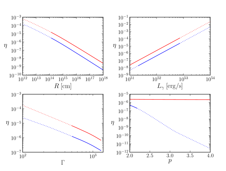
Figure 1: A plot of the maximum efficiencies for the photo-pion process radiating a typical Fermi-LAT flux of 1 $\mu$Jy at 100 MeV as a function of $R$, $L$, $\Gamma,$ and $p$. The lower blue lines corresponds to a more physically realistic case of a proton power law extending from a Lorentz factor of 10 to the Hillas criterion for the confinement of protons. The upper red lines are the efficiency only considering the energy in the protons that produce the pions and then electrons that radiate at LAT frequencies. These red lines represent an absolute maximum possible efficiency and corresponds roughly to our calculation in §2.1. The dotted line corresponds to the cases when LAT emission could not be seen by an observer, either because the emission happens below the photosphere or because the jet would be opaque to photons of 10 GeV due to $\gamma+\gamma$ pair production. In a two zone model for gamma-ray generation, the area where this occurs may differ by a small factor. When the parameters are not on the $x$-axis, values of $L_{\gamma}=10^{52}$ erg/s, $R=10^{15}$ cm, $\Gamma=800$, $\nu_{p}=1$ MeV, $z=2$, $d_{L}=4.9\times 10^{28}$ cm, and $p=2$ are taken. The photon power law indices of the Band function were set to $\alpha=1$ and $\beta=2.2$. Since $\nu_{p},$ $\alpha,$ and $\beta$ are unable to change the maximum $\eta$ by more than an order of magnitude, their corresponding plots are omitted.

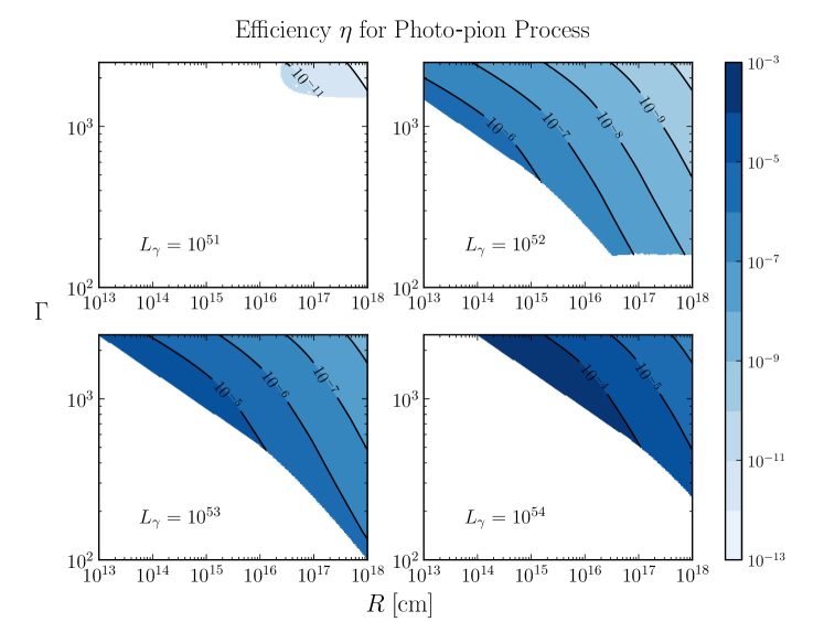
Figure 2: The maximum $\eta$ is plotted in the $R-\Gamma$ plane for various values of $L_{\gamma}$ to match a flux of $f_{\nu}=1\ \mu{\rm Jy}$ at 100 MeV. As in Figure 1, we fix $\nu_{p}=1$ MeV, $z=2$, $d_{L}=4.9\times 10^{28}$ cm, and $p=2$. The photon power law indices were set to typical values for the Band function, $\alpha=1$ and $\beta=2.2$. Where $\eta$ is not shown, the place of emission is either below the photosphere or opaque to radiation of 10 GeV due to $\gamma+\gamma$ pair production.

3 Bethe-Heitler Pair Production

Through Bethe-Heitler pair production, protons and photons interact to create electron-position pairs directly, $p+\gamma\rightarrow p+e^{+}+e^{-}$. The Bethe-Heitler cross-section and the energy of the produced electron-positron pair depend strongly on the angle between the outgoing electron/positron and the proton. Therefore, it is not possible to use the integrated cross section to calculate the secondary electron production. Assuming that the protons and photons are isotropic in the jet’s rest frame and using the head on approximation, i.e. the angle between the photon and proton is zero, i.e. $\epsilon^{\prime}=2\gamma_{p}\epsilon$, the equation for the rate of production of secondary electrons is:

$$\frac{d\dot{N}_{e}}{d\gamma_{e}}(\gamma_{e})=2c\int_{0}^{\infty}{d\epsilon\ n(\epsilon)\int_{1}^{\infty}{d\gamma_{p}\ N_{p}(\gamma_{p})\frac{d\sigma(\epsilon,\gamma_{p})}{d\gamma_{e}}}}.$$ (49)

In this equation $N_{p}(\gamma_{p})$ is the number of protons with Lorentz factor $\gamma_{p}$ and $n(\epsilon)$ is number density of photons with energy $\epsilon$. The formula for the differential Bethe-Heitler cross section, $\sigma_{BH}$, in the Born approximation, integrated over angles in the highly relativistic regime, was derived by Bethe & Maximon (1954) (see Rachen (1996) for a more recent review).

$$\frac{d\sigma_{BH}}{d\gamma^{\prime}_{+}}=\frac{3\alpha_{f}\sigma_{T}}{2\pi{\epsilon^{\prime}}^{3}}\left({\gamma_{+}^{\prime}}^{2}+{\gamma_{-}^{\prime}}^{2}+\frac{2}{3}\gamma_{+}^{\prime}\gamma^{\prime}_{-}\right)\left(\log{\frac{2\gamma^{\prime}_{+}\gamma^{\prime}_{-}}{\epsilon^{\prime}}}-\frac{1}{2}\right).$$ (50)

In this equation, $\gamma^{\prime}_{+}(\gamma^{\prime}_{-})$ is the Lorentz factor of the positron (electron), $\alpha_{f}$ is the fine structure constant, and all of the above quantities are in the proton rest frame. Much of the contribution to the angle-integrated cross section comes from angles between the photon and outgoing $e^{\pm}$ of order $\theta^{\prime}_{\pm}=\frac{1}{\gamma_{\pm}^{\prime}}$. When $\gamma_{p}\gg\gamma^{\prime}_{\pm}$, the Lorentz factor of $e^{\pm}$ in the jet’s rest frame is

$$\gamma_{\pm}=\gamma_{p}\gamma_{\pm}^{\prime}\left(1-\beta_{p}\beta^{\prime}_{\pm}\cos{\theta^{\prime}_{\pm}}\right)\approx\frac{\gamma_{p}\gamma_{\pm}^{\prime}}{2}\left(\gamma_{p}^{-2}+{\gamma_{\pm}^{\prime}}^{-2}+{\theta^{\prime}_{\pm}}^{-2}\right)\approx\frac{\gamma_{p}}{\gamma^{\prime}_{\pm}}.$$ (51)

Therefore, most pairs produced via the Bethe-Heitler process have Lorentz factors (in the jet comoving frame) that are smaller than the proton that created it.

If $\epsilon^{\prime}\ll m_{p}/m_{e}\sim 10^{3}$, the nuclear recoil of the proton can be neglected and the following equality holds:

$$\gamma^{\prime}_{+}+\gamma^{\prime}_{-}=\epsilon^{\prime}.$$ (52)

For large $\epsilon^{\prime}$, the differential cross section decreases very rapidly when $\gamma_{\pm}^{\prime}<2$. Therefore, we only consider $\gamma_{\pm}^{\prime}\geq 2$, where the differential cross section is more or less constant. In this regime, the differential cross section simplifies to

$$\frac{d\sigma_{BH}}{d\gamma^{\prime}_{+}}\approx\frac{\alpha\sigma_{T}}{\epsilon^{\prime}},\mbox{ if }2\leq\gamma_{+}^{\prime}\leq\epsilon^{\prime}-2.$$ (53)

Re-writing eq (53) in the jet comoving frame and using the $\epsilon^{\prime}\approx 2\gamma_{p}\epsilon$, we find

$$\frac{d\sigma_{BH}}{d\gamma_{+}}\approx\frac{\alpha\sigma_{T}}{2\epsilon\gamma_{+}^{2}},\mbox{ if }\frac{1}{2\epsilon}\leq\gamma_{+}\leq\frac{\gamma_{p}}{2}.$$ (54)

The integral in equation (49) is simplified by considering this approximate expression for the cross-section. The integral is now straight forward to calculate for a Band spectrum with indices $\alpha$, $\beta$ and a proton index of $p$. The result is

$$\frac{d\dot{N}_{e}}{d\gamma_{e}}(\gamma_{e})\approx\left\{\begin{array}[]{ll}\hskip-5.0pt\frac{2c\alpha_{f}\sigma_{T}}{\beta(p+1)\gamma_{e}}n_{\epsilon_{p}}N_{p,i}\left(\frac{\gamma_{e}\epsilon_{p}}{5}\right)^{\beta}\left(\frac{2\gamma_{e}}{\gamma_{i}}\right)^{-p}&\mbox{for }\frac{\gamma_{i}}{2}\leq\gamma_{e}\leq 5/\epsilon_{p}\\ \\ \hskip-5.0pt\frac{2c\alpha_{f}\sigma_{T}\epsilon_{p}}{5\beta(p+1)}n_{\epsilon_{p}}N_{p,i}\left(\frac{10}{\epsilon_{p}\gamma_{i}}\right)^{-p}\left(\frac{\epsilon_{p}\gamma_{e}}{5}\right)^{\alpha-p-1}&\mbox{for }5/\epsilon_{p}\leq\gamma_{e}\leq 5/\epsilon_{\rm min}.\end{array}\right.$$ (55)

We now compare Bethe-Heitler pair production to the photo-pion process. The integrated cross section for Bethe-Heitler process is roughly 10 times larger than the cross section for the photo-pion $\Delta$-resonance. For any given proton Lorentz factor $\gamma_{p}$, the photon energy required for Bethe-Heitler is roughly 50 times smaller than for the $\Delta$-resonance. For a given $\gamma_{p}$, the photo-pair will have an average Lorentz factor of $\sim\gamma_{p}/5$ while the delta resonance will decay to a electron with an energy $\sim 70\gamma_{p}$. Consider the case where protons with a power-law distribution function with index $p$ are scattering with a isotropic photon power-law spectrum $n(\epsilon)\propto\epsilon^{-a}$. The ratio of the number of $e^{\pm}$ above a fixed Lorentz factor generated by Bethe-Heitler process compared to those generated by photo-pion process is $\sim 2\times 10\times(10^{4})^{a-1}\times(300)^{-p+1}$—the first factor comes from the fact that Bethe-Heitler produces a electron-positron pair compared to a single positron produced in the delta-resonance, the second factor is the ratio of the total cross sections for the Bethe-Heitler and photo-pion scatterings, the third factor accounts for the larger number of photons that participate in the Bethe-Heitler process (the threshold energy for Bethe-Heitler is $\epsilon\sim\gamma_{e}^{-1}$ and the threshold energy for photo-pion is $\sim 10^{4}\gamma_{e}^{-1}$) and the final factor is due to the fewer number of protons that can create electrons with Lorentz factor $\ga\gamma_{e}$. This means that which process dominates depends strongly on which part of the Band function the protons are interacting with to produce $e^{\pm}$ with Lorentz factor $\ga\gamma_{e}$. For $\gamma_{e}\ga 10^{6}$, the energy threshold for both processes lies below the peak of the Band function, so $a=\alpha\approx 1$. Thus, in this regime, the photo-pion pairs dominate.

However, for $\gamma_{e}\la 10^{3}$, the threshold photon energy for both process is above the peak of the gamma ray spectrum, so $a=\beta\approx 2.2$ and the Bethe-Heitler process is a lot more efficient than the photo-pion process. Although relativistic shocks are likely capable of accelerating electrons to $\gamma_{e}\sim 10^{3}$, Bethe-Heitler process could still be important if the number of electrons produced above the photosphere vastly outnumber the electrons expected to be in the GRB jet from simple charge neutrality. If the GRB has proton luminosity $L_{p}$ given by $L_{p}=\eta^{-1}L_{\gamma}$, the comoving electron density is $n_{e}=n_{p}\approx 2\times 10^{9}\eta^{-1}L_{\gamma,52}\Gamma_{2}^{-2}R_{15}^{-2}\ {\rm cm^{-3}}$. The number density of Bethe-Heitler produced electrons, $n_{BH}$ is

$$n_{BH}\sim\alpha_{f}\sigma_{T}n_{\gamma}n_{p}R/\Gamma\quad\Rightarrow\quad\frac{n_{BH}}{n_{e}}=\alpha_{f}\sigma_{T}n_{\gamma}R/\Gamma.$$ (56)

Since we want to restrict ourselves to above the photosphere, the optical depth $\sigma_{T}n_{e}R/\Gamma<1$ or

$$\frac{n_{BH}}{n_{e}}<\alpha_{f}\frac{n_{\gamma}}{n_{e}}\sim 10^{3}\eta\Gamma_{2}\nu_{p,6}^{-1}(1+z)^{-1},$$ (57)

where $n_{\gamma}$ is given by eq (6). It is somewhat counter-intuitive, but the Bethe-Heitler process is likely to be most important in jets with lower baryon loading, i.e. when $\eta$ is large. The Bethe-Heitler process could be important for $\gamma_{e}^{\prime}\ll 10^{5}$—especially if for some reason the Fermi mechanism is unable to accelerate electrons to this Lorentz factor in GRB shocks—but for these $e^{\pm}$ to account for the 100 MeV photons from GRBs via the synchrotron process requires a very large magnetic field and the luminosity carried by such a magnetic field would greatly exceed 10⁵² erg/s. Therefore, it seems that at best there might just be a small part of the parameter space for GRBs where the Bethe-Heitler mechanism could play an interesting role in the generation of prompt $\gamma$-ray radiation.

4 Proton Synchrotron

Massive particles have lower radiative losses than lighter particles, and therefore more massive particles are easier to accelerate in shocks. The maximum Lorentz factor that protons can attain is much larger than the maximum Lorentz factor of electrons. The maximum synchrotron photon energy from a shock-accelerated particle is given by requiring that the synchrotron energy radiated during one acceleration time (on the order of the Larmor time) is equal the energy gained in an acceleration cycle—half of the particle’s energy. i.e. $\gamma mc/(qB)\times 4B^{2}q^{4}\gamma^{2}/(9m^{2}c^{3})\la\gamma mc/2$. The maximum photon energy for a source moving with a Lorentz factor $\Gamma$ at redshift $z$ is

$$\nu_{\rm max}\approx\frac{9\Gamma mc^{3}}{16\pi q^{2}(1+z)}\sim 50\frac{\Gamma}{1+z}\left(\frac{m}{m_{e}}\right)\ {\rm MeV}.$$ (58)

While electron synchrotron radiation can only produce photons up to an energy $\sim 50\Gamma/(1+z)$ MeV, the proton synchrotron process can radiate photons up to $10^{2}\Gamma/(1+z)$ GeV. For this reason, when photons of energies larger than what is allowed by electron synchrotron are detected from a source, proton synchrotron is frequently suggested as a possible radiation mechanism (e.g. Bottcher & Dermer, 1998; Totani, 1998; Aharonian, 2000; Zhang & Mészáros, 2001; Mücke et al., 2003; Reimer et al., 2004; Razzaque et al., 2010).

However, while the lower radiative efficiency of protons allows the protons to radiate at higher frequencies, it also means that the proton-synchrotron model requires more energy in the magnetic field to match an observed flux. Because of this, we find that to match the typical observations of Fermi-LAT GRBs, either the energy requirements are prohibitive or the proton power-law distribution would have to begin at extremely high Lorentz factors.

As before, we are considering protons with a power-law distribution $dN_{p}(\gamma_{p})\propto\gamma_{p}^{-p}\ d\gamma_{p}$ if $\gamma_{p}\geq\gamma_{i}$. The proton injection frequency, $\nu_{i}$, is

$$\nu_{i}=\frac{qB\Gamma\gamma_{i}^{2}}{2\pi m_{p}c(1+z)}\approx 6.3\times 10^{-10}B\Gamma_{2}\gamma_{i}^{2}(1+z)^{-1}\ {\rm eV}.$$ (59)

We define the cooling frequency, $\nu_{c}$, as the frequency where the synchrotron cooling time of the protons that radiate at $\nu_{c}$ is equal to the dynamical time. The cooling time for protons is increased by a factor $\left(\frac{m_{p}}{m_{e}}\right)^{3}$ compared to the cooling time of electrons. The cooling frequency for proton synchrotron is

$$\nu_{c}\approx 5\times 10^{23}B^{-3}R_{15}^{-2}\Gamma^{3}_{2}(1+z)^{-1}\ {\rm eV}.$$ (60)

Since nearly all GRB observed in the Fermi-LAT band have a spectrum that can be fit by a single power law in the LAT band, we examine two possible spectral orderings: $\nu_{i}\sim\nu_{c}\leq\nu$ and the slow cooling regime $\nu_{i}\leq\nu\leq\nu_{c}$.

$\nu$ must be above $\nu_{i}$ to match the spectra of Fermi-LAT GRBs: $\nu\leq\nu_{i}$ cannot produce GRB LAT emission because if the protons are cooled (uncooled), the spectrum is $f_{\nu}\propto\nu^{-1/2}\ (\nu^{1/3})$. These spectra are harder than what is observed for most GRB, which have a typical high energy $f_{\nu}$ index $<-1$ (Ackerman et al., 2012). Therefore, we take $\nu_{i}\leq\nu$ to agree with a typical GRB spectrum. The synchrotron flux $f_{\nu}$ at the peak of the spectrum ($\nu_{i}=\min{(\nu_{i},\nu_{c})}$) is

$$f_{\nu}\approx 7BN_{52}\Gamma_{2}(1+z)d^{-2}_{L,28}\ \mu{\rm Jy},$$ (61)

where N is the total number of protons radiating in a dynamical time. The flux scales as $f_{\nu}\propto\nu^{-\frac{p-1}{2}}$ if $\nu_{i}\leq\nu\leq\nu_{c}$ and as $f_{\nu}\propto\nu^{-\frac{p}{2}}$ if $\nu\geq\nu_{c},\nu_{i}$.

Below $\nu_{p}$, the flux of a typical GRB is constant, $f_{\nu}\propto\nu^{0}$. Above $\nu_{p}$, the flux scales as $f_{\nu}\propto\nu^{-1.2}$. Since this break is larger than one half, it cannot be attributed to a cooling break. Therefore, in order to have $f_{\nu}\propto\nu^{0}$ below $\nu_{p}$, we require that both $\nu_{i}$ and $\nu_{c}$ lie above $\nu_{p}$. Furthermore, the majority of LAT GRBs show a single power law above their peak, extending up to a maximum observed frequency, $\nu_{\rm max}$, on the order of tens of GeV. We need to ensure that the proton synchrotron radiation does not add any spectral features in this energy range. Since we have already ruled out the fast-cooling regime, there are only two possibilities: the cooled case where, $\nu_{i}\sim\nu_{c}\sim\nu_{p}\sim 1\ {\rm MeV}$ with a $p\sim 2.4$ and the uncooled case where $\nu_{i}\sim\nu_{p}$, $\nu_{c}\ga\nu_{\rm max}$ with $p\sim 3.4$. The cooled case can be ruled out because the energy required in the magnetic field is far too large. The uncooled case is considered in more detail in the following paragraphs.

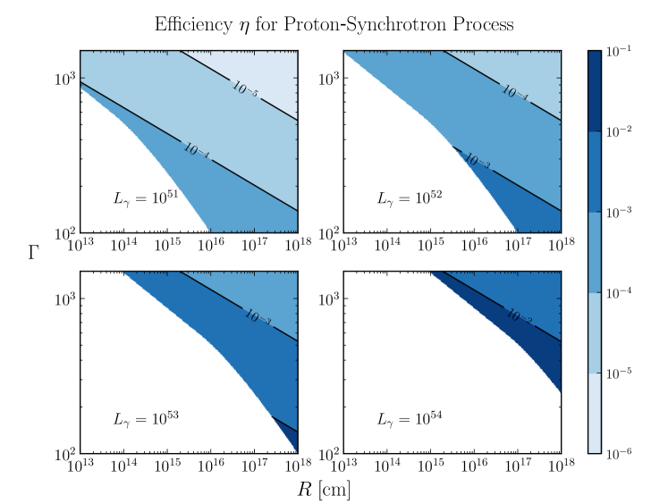
Figure 3: The maximum $\eta\equiv L_{\gamma}/(L_{p}+L_{B})$ plotted in the $R-\Gamma$ plane for various values of $L_{\gamma}$ to match a flux of $f_{\nu}=1\ \mu{\rm Jy}$ at 100 MeV. As in the previous figures, we fix $z=2$, and $d_{L}=4.9\times 10^{28}$ cm. This $\eta$ corresponds to the necessary luminosity in magnetic field and protons with energies greater than $\sim 4\Gamma$ PeV to match a flux of $f_{\nu}=1\ \mu{\rm Jy}$ at 100 MeV. The luminosity in protons with lower energies is likely comparable or much larger. Even when not considering the lower energy protons, the efficiency is very small for a vast majority of GRB parameter space. When $\eta$ is not shown either the place of emission is below the photosphere or it is opaque to radiation of 10 GeV due to $\gamma+\gamma$ pair production.

If we require that $\nu_{i}\sim\nu_{8}$ (i.e. 100 MeV) and $\nu_{c}\ga\nu_{\rm max}\sim 10$ GeV, we can then place an upper bound on the magnetic field by requiring that $\nu_{c}>\nu_{\rm max}$ and a lower bound by requiring that protons will be able to be accelerated to high enough energies to radiate at $\nu_{\rm max}$. As a practical matter, these bounds do not affect our maximally efficient proton-synchrotron radiation calculation for the parameter range considered. We then minimize the total luminosity required in both the magnetic field and protons radiating at an observed frequency $\nu_{8}$ to match a typical observed flux of a few $\mu$Jy.

The minimum Lorentz factor of the proton that radiates at $\nu_{8}$ is

$$\gamma_{i}=4\times 10^{8}B^{-1/2}\Gamma_{2}^{-1/2}(1+z)^{1/2}\nu_{8}^{1/2}.$$ (62)

This Lorentz factor gives a proton luminosity $L_{p}$ of

$$L_{p}=2\Gamma^{3}\gamma_{i}R^{-1}m_{p}c^{3}N\approx 5\times 10^{58}f_{\nu,\mu{\rm Jy}}B^{-3/2}\Gamma_{2}^{3/2}R_{15}^{-1}\nu_{8}^{1/2}(1+z)^{-1/2}d_{L,28}^{2}\ {\rm erg/s}.$$ (63)

Given the magnetic field luminosity, $L_{B}=6\times 10^{44}B^{2}R_{15}^{2}\Gamma_{2}^{2}$ erg/s, the total luminosity $L_{B}+L_{p}$ will be minimized with respect to $B$ when $L_{p}=\frac{4}{3}L_{B}$, or when

$$B\approx 10^{4}\ \Gamma_{2}^{-1/7}R_{15}^{-6/7}f_{\nu,\mu{\rm Jy}}^{2/7}\nu_{8}^{1/7}(1+z)^{-1/7}d_{L,28}^{4/7}\ {\rm Gauss}.$$ (64)

This magnetic field gives a proton luminosity

$$L_{p}=\frac{4}{3}L_{B}\approx 5\times 10^{52}f_{\nu,\mu{\rm Jy}}^{4/7}\Gamma_{2}^{12/7}R_{15}^{2/7}\nu_{8}^{2/7}(1+z)^{-2/7}d_{L,28}^{8/7}\ {\rm erg/s}.$$ (65)

The efficiency $\eta$ is plotted in figure 3. Note that $L_{B}$ is not negligible as in figure 1 and 2, so in figure 3, $\eta\equiv L_{\gamma}/(L_{p}+L_{B})$. The proton luminosity is much larger than the $\gamma$-ray luminosity for most of the allowed GRB parameter space. Additionally, proton synchrotron requires an unrealistically large $\gamma_{i}$. Using eq (64),

$$\gamma_{i}\approx 4\times 10^{6}\ R_{15}^{3/7}\Gamma_{2}^{-3/7}(1+z)^{4/7}\nu_{8}^{3/7}f_{\nu,\mu{\rm Jy}}^{-1/7}d_{L,28}^{-2/7}.$$ (66)

It is unclear what physical process could produce a power law with such a high minimum Lorentz factor. The minimum Lorentz factor of a particle accelerated in relativistic shocks is approximately equal to the Lorentz factor of the shock front with respect to the unshocked fluid, if every proton crossing the shock front is accelerated. The Lorentz factor can be proportionally larger if a small fraction of particles are accelerated and the remaining particles are “cold” downstream of the shock front. Considering that the Lorentz factor for GRB internal shocks is of order a few to perhaps a few tens, the typical proton Lorentz factor should be $\sim 10-10^{3}$ (the larger value corresponds to when only 1 in $10^{2}$ protons are accelerated, as suggested by simulations, e.g. Sironi & Spitkovsky (2011)). $\gamma_{i}\sim 4\times 10^{6}$ is an unrealistically high injection Lorentz factor for relativistic shocks. If we set $\gamma_{i}$ to $10^{3}$, the proton synchrotron radiation would extend down to $\sim 1$ keV and would over produce in the GBM band. We can only decrease $\gamma_{i}$ by a factor of 10 before over producing below the peak of the GRB spectrum. In summary, if proton synchrotron is to explain the observed LAT emission in GRBs, all of the protons must be accelerated to extremely high Lorentz factors very efficiently by some unknown mechanism.

The expected neutrino flux for the proton synchrotron model is estimated below. The total number of muon neutrinos is $\sim 2\tau_{p\gamma}N_{p}$, where $\tau_{p\gamma}$ is the optical depth to photo-pion production, given in eq (7), and $N_{p}$ is calculated using eq (61) and (64):

$$N_{\nu}=2\times 10^{47}L_{\gamma,52}\Gamma_{2}^{-20/7}R_{15}^{-1/7}f_{\nu,{\rm\mu Jy}}^{5/7}\nu_{p,6}^{-1}(1+z)^{-13/7}\nu_{8}^{-1/7}d_{L,28}^{10/7}.$$ (67)

Because the proton synchrotron radiation requires higher energy protons and larger magnetic fields compared to the photo-pion process, the pions produced will suffer larger radiative losses from synchrotron radiation before they decay. If the magnetic field is given by eq (64) we find that the pions will be cooled significantly by synchrotron radiation when $\Gamma_{2}^{12/7}R_{15}^{2/7}<4f_{\nu,{\rm\mu Jy}}^{3/7}\nu_{8}^{5/7}(1+z)^{2/7}d_{L,28}^{6/7}$. The neutrino flux will peak at an observed energy of $\sim\frac{1}{4}\Gamma\gamma_{i}m_{\pi}c^{2}/(1+z)$ if the pions are uncooled. If the pions are cooled, the flux will peak at the energy where pion cooling becomes important,or an energy of $\sim\frac{1}{4}\Gamma\gamma_{\pi,{\rm cool}}m_{\pi}c^{2}/(1+z)$ ($\gamma_{\pi,cool}\equiv 10^{14}B^{-2}\Gamma_{2}R_{15}^{-1}$).

$$E_{\nu}=\left\{\begin{array}[]{ll}\hskip-5.0pt1.4\times 10^{7}\ \Gamma_{2}^{4/7}R_{15}^{3/7}f_{\nu,\mu{\rm Jy}}^{-1/7}\nu_{8}^{3/7}(1+z)^{-3/7}d_{L,28}^{-2/7}\ {\rm GeV}&\mbox{if pions are not cooled}\\ \\ \hskip-5.0pt3.5\times 10^{6}\Gamma_{2}^{16/7}R_{15}^{5/7}f_{\nu,\mu{\rm Jy}}^{-4/7}\nu_{8}^{-2/7}(1+z)^{-5/7}d_{L,28}^{-8/7}{\rm GeV}&\mbox{if pions are cooled}\end{array}\right.$$ (68)

Since the protons are not cooled by the synchrotron loss mechanism, the observed neutrino flux is calculated using eq (16) and the dynamical time. The neutrino flux, $F_{\nu}$, peaks at an energy given by eq (68) and is

$$F_{\nu}=\left\{\begin{array}[]{ll}\hskip-5.0pt1.4\times 10^{-3}\ L_{\gamma,52}\Gamma_{2}^{-2/7}R_{15}^{-5/7}\nu_{p,6}^{-1}\nu_{8}^{2/7}f_{\nu,\mu{\rm Jy}}^{4/7}d_{L,28}^{-6/7}(1+z)^{-9/7}\ {\rm GeV\ cm^{-2}s^{-1}}&\mbox{if pions are not cooled}\\ \\ \hskip-5.0pt3.3\times 10^{-4}\ L_{\gamma,52}\Gamma_{2}^{10/7}R_{15}^{-3/7}\nu_{p,6}^{-1}\nu_{8}^{-3/7}f_{\nu,\mu{\rm Jy}}^{1/7}d_{L,28}^{-12/7}(1+z)^{-11/7}\ {\rm GeV\ cm^{-2}s^{-1}}&\mbox{if pions are cooled.}\end{array}\right.$$ (69)

As in Section 2.1.1, we estimate the neutrinos detected by IceCube per second of LAT emission from the proton synchrotron process:

$$\frac{dN_{\nu}}{dt}=\left\{\begin{array}[]{ll}\hskip-5.0pt10^{-3}\ L_{\gamma,52}\Gamma_{2}^{-4/7}R_{15}^{-13/14}f_{\nu,{\rm\mu Jy}}^{9/14}\nu_{8}^{1/14}\nu_{p,6}^{-1}d_{L,28}^{-5/7}(1+z)^{-15/14}\ {\rm counts\ s^{-1}}&\mbox{if the pions are not cooled}\\ \\ \hskip-5.0pt5.6\times 10^{-4}\ L_{\gamma,52}\Gamma_{2}^{2/7}R_{15}^{-11/14}f_{\nu,{\rm\mu Jy}}^{3/7}\nu_{8}^{-2/7}\nu_{p,6}^{-1}d_{L,28}^{-8/7}(1+z)^{-17/14}\ {\rm counts\ s^{-1}}&\mbox{if the pions are cooled.}\end{array}\right.$$ (70)

Therefore, for a bright GRB detected by the Fermi-LAT with $L_{\gamma,52}\sim 10$, $f_{\nu},{\rm\mu Jy}\sim 2$, $\Gamma_{2}\sim 9$, $z\sim 2$ and $\nu_{p,6}\sim 1$ and a duration of 10 seconds we find that the pions will be cooled if $R<2\times 10^{14}\ {\rm cm}$. We expect $\sim 4\times 10^{-3}R_{15}^{-13/14}$ neutrinos of energy $2\times 10^{7}R_{15}^{3/7}\ {\rm GeV}$ if $R>2\times 10^{14}{\rm cm}$ and $\sim 6\times 10^{-3}R_{15}^{-11/14}$ neutrinos of energy $2.7\times 10^{7}R_{15}^{5/7}\ {\rm GeV}$ if $R<2\times 10^{14}{\rm cm}$.

5 Summary and Discussion

With a goal of understanding typical observed 100 MeV fluxes in bright Fermi-LAT GRBs during the prompt emission, we estimated the generation of photons by high-energy protons traveling through a shell of photons whose energy distribution is given by the Band function. We calculated the minimum energy in protons required to reproduce Fermi-LAT observations for the following hadronic processes: photo-pion, Bethe-Heitler pair production, and proton synchrotron.

Unlike previous works, we specifically focused on the energy required for hadronic models to produce the $>$100 MeV photons seen in Fermi GRBs and how this requirement depends on GRB parameters. To provide additional physical insight into the energy requirements, we have provided both analytical estimates and more detailed numerical calculations.

We find that photo-pion $\Delta$-resonance is much more efficient than Bethe-Heitler pair production at producing high-energy electrons—so much so that Bethe-Heitler pair production can be ruled out as a mechanism for producing $\ga 100$ MeV photons observed by Fermi-LAT. The photo-pion process is capable of producing high energy electrons, but to match the Fermi-LAT flux at 100 MeV, the photo-pion process requires an energy in protons that is $\ga 10^{4}$ times greater than isotropic energy in the $\gamma$-ray photons. Since the Bethe-Heitler photo-pairs are produced more efficiently at low energies, Bethe-Heitler production will be the dominant process at low energies. These low-energy Bethe-Heitler electrons will have the same spectral index as the high-energy photo-pion electrons (assuming there isn’t a cooling break). Therefore it is possible that both processes could add up to produce a single power-law deviation from the Band function that extends from low to high energies. This type of spectral feature has been observed in several Fermi GRBs.

According to our calculations, proton synchrotron is capable of producing the Fermi-LAT GRB emission more efficiently than the other hadronic processes. The proton synchrotron could possible achieve efficiencies on the order of 1-10% for the brightest GRBs, if we assume that the minimum Lorentz factor for proton accelerated in shocks is extremely large $\sim 2\times 10^{6}$. The minimum proton Lorentz factor of order $10^{6}$ is much larger than what is expected based on our current understanding of relativistic collisionless shocks. Regardless of the mechanism accelerating the protons, these high energy protons with LF greater than $10^{6}$ likely carry only a small fraction of the total energy carried by the protons.

We also calculated the expected neutrino flux if the LAT emission is from the photo-pion process or proton synchrotron radiation. In the photo-pion process, for a bright LAT GRB with a Lorentz Factor of 900 and a duration of 10 seconds, we expect $\sim.1$ neutrinos detected by IceCube at an energy of $\sim 10^{6}\ {\rm GeV}$. Therefore, it may be possible to rule out photo-pion emission when the emission from multiple bursts is considered. For proton synchrotron radiation, the neutrino flux also depends on the emission radius, $R$. For a bright LAT GRB with a Lorentz factor of 900, an emission radius of $10^{15}$ cm and duration of 10 seconds, we expect a $\sim 4\times 10^{-3}$ neutrinos detected by IceCube at an energy $\sim 2\times 10^{7}\ {\rm GeV}$.

In summary, all the hadronic processes considered in this paper require significantly more energy in protons than the observed energy in gamma-rays to reproduce the high-energy flux observed in Fermi-LAT GRBs.

6 Acknowledgments

This work has been funded in part by NSF grant ast-0909110, and a Fermi-GI grant (NNX11AP97G). Patrick would like to thank Rodolfo Barniol Duran and Rodolfo Santana for their helpful discussions and his wife Diana for her support and help preparing the paper.

References

- Abbasi et al. (2012) Abbasi R., Abdou Y., Abu-Zayyad T., Ackermann M., Adams J., Aguilar J. A., Ahlers M., Altmann D., Andeen K., Auffenberg J., et al., 2012, Nature, 484, 351
- Abdo et al. (2009a) Abdo A. A., et al., 2009a, ApJ, 706, L138
- Abdo et al. (2009b) Abdo A. A., et al., 2009b, Science, 323, 1688
- Ackerman et al. (2012) Ackerman M., et al., 2012, ApJ, 754, 121
- Ackermann et al. (2011) Ackermann M., et al., 2011, ApJ, 729, 114
- Aharonian (2000) Aharonian F. A., 2000, New Astronomy, 5, 377
- Asano et al. (2009) Asano K., Guiriec S., Mészáros P., 2009, ApJ, 705, L191
- Asano et al. (2010) Asano K., Inoue S., Mészáros P., 2010, ApJ, 725, L121
- Asano & Mészáros (2012) Asano K., Mészáros P., 2012, ArXiv:1206.0347
- Atwood et al. (2009) Atwood W. B., Abdo A. A., et al., 2009, ApJ, 697, 1071
- Band et al. (1993) Band D., et al., 1993, ApJ, 413, 281
- Bell (1978) Bell A. R., 1978, MNRAS, 182, 147
- Bethe & Maximon (1954) Bethe H. A., Maximon L. C., 1954, Physical Review, 93, 768
- Blandford & Eichler (1987) Blandford R., Eichler D., 1987, Phyiscs Reports, 154, 1
- Blandford & Ostriker (1978) Blandford R. D., Ostriker J. P., 1978, ApJ, 221, L29
- Blumenthal (1971) Blumenthal G. R., 1971, Phys. Rev. D, 3, 2308
- Bottcher & Dermer (1998) Bottcher M., Dermer C. D., 1998, ApJ, 499, L131
- Corsi et al. (2010) Corsi A., Guetta D., Piro L., 2010, ApJ, 720, 1008
- de Jager et al. (1996) de Jager O. C., Harding A. K., Michelson P. F., Nel H. I., Nolan P. L., Sreekumar P., Thompson D. J., 1996, ApJ, 457, 253
- Drenkhahn & Spruit (2002) Drenkhahn G., Spruit H. C., 2002, A&A, 391, 1141
- Fan & Piran (2006) Fan Y., Piran T., 2006, MNRAS, 369, 197
- Gao et al. (2009) Gao W.-H., Mao J., Xu D., Fan Y.-Z., 2009, ApJ, 706, L33
- Greiner et al. (2009) Greiner J., Clemens C., Krühler T., et al., 2009, A&A, 498, 89
- Hascoët et al. (2012) Hascoët R., Daigne F., Mochkovitch R., Vennin V., 2012, MNRAS, 421, 525
- Hillas (1984) Hillas A. M., 1984, ARA&A, 22, 425
- Kumar & Barniol Duran (2009) Kumar P., Barniol Duran R., 2009, MNRAS, 400, L75
- Kumar & Barniol Duran (2010) Kumar P., Barniol Duran R., 2010, MNRAS, 409, 226
- Lithwick & Sari (2001) Lithwick Y., Sari R., 2001, ApJ, 555, 540
- Lyutikov (2006) Lyutikov M., 2006, New Journal of Physics, 8, 119
- Lyutikov & Blandford (2003) Lyutikov M., Blandford R., 2003, ArXiv:031247
- Maxham et al. (2011) Maxham A., Zhang B.-B., Zhang B., 2011, MNRAS, 415, 77
- Mücke et al. (2003) Mücke A., Protheroe R. J., Engel R., Rachen J. P., Stanev T., 2003, Astroparticle Physics, 18, 593
- Murase et al. (2012) Murase K., Asano K., Terasawa T., Mészáros P., 2012, ApJ, 746, 164
- Panaitescu & Kumar (2002) Panaitescu A., Kumar P., 2002, ApJ, 571, 779
- Rachen (1996) Rachen J., 1996, PhD thesis, University of Bonn
- Rachen & Mészáros (1998) Rachen J. P., Mészáros P., 1998, Phys. Rev. D, 58, 123005
- Razzaque et al. (2010) Razzaque S., Dermer C. D., Finke J. D., 2010, The Open Astronomy Journal, 3, 150
- Reimer et al. (2004) Reimer A., Protheroe R. J., Donea A.-C., 2004, New Astronomy Review, 48, 411
- Sironi & Spitkovsky (2011) Sironi L., Spitkovsky A., 2011, ApJ, 726, 75
- Totani (1998) Totani T., 1998, ApJ, 509, L81
- Usov (1992) Usov V. V., 1992, Nature, 357, 472
- Zhang et al. (2007) Zhang B., et al., 2007, ApJ, 655, 989
- Zhang & Mészáros (2001) Zhang B., Mészáros P., 2001, ApJ, 559, 110
- Zhang et al. (2011) Zhang B.-B., Zhang B., Liang E.-W., Fan Y.-Z., Wu X.-F., Pe’er A., Maxham A., Gao H., Dong Y.-M., 2011, ApJ, 730, 141
- Zou et al. (2011) Zou Y.-C., Fan Y.-Z., Piran T., 2011, ApJ, 726, L2