Do globular clusters possess Dark Matter halos?
A case study in NGC 2419
Abstract
We use recently published measurements of the kinematics, surface brightness and stellar mass-to-light ratio of the globular cluster NGC 2419 to examine the possibility that this Galactic halo satellite is embedded in a low-mass dark matter halo. NGC 2419 is a promising target for such a study, since its extreme Galactocentric distance and large mass would have greatly facilitated the retention of dark matter. A Markov-Chain Monte Carlo approach is used to investigate composite dynamical models containing a stellar and a dark matter component. We find that it is unlikely that a significant amount of dark matter ( of the luminous mass inside the tidal limit of the cluster) can be present if the stars follow an anisotropic Michie model and the dark matter a double power law model. However, we find that more general models, derived using a new technique we have developed to compute non-parametric solutions to the spherical Jeans equation, suggest the presence of a significant dark matter fraction (approximately twice the stellar mass). Thus the presence of a dark matter halo around NGC 2419 cannot be fully ruled out at present, yet any dark matter within the 10′ visible extent of the cluster must be highly concentrated and cannot exceed (99% confidence), in stark contrast to expectations for a plausible progenitor halo of this structure.
keywords:
globular clusters: individual (NGC 2419) — dark matter — stellar dynamics1 Introduction
Dwarf spheroidal galaxies (dSphs) and globular clusters (GCs) have similar luminosities but are strikingly different in terms of their dark-matter (DM) content, as inferred from the kinematics of their stars: while dSphs (and their “ultra-faint” extension to low luminosity) galaxies are the most DM dominated systems, there is virtually no evidence that GCs have DM halos (Heggie & Hut, 1996; Mashchenko & Sills, 2005a; Bradford et al., 2011). This finding might represent a problem for standard cold dark matter cosmology, in which GCs are expected to form within their own DM halos (Peebles, 1984). However it is quite possible that GCs were originally embedded in massive DM halos that evolved during the cluster lifetime as a consequence of interaction with the cluster stars (Baumgardt & Mieske, 2008) and stripping by the tidal field of the host galaxy (Mashchenko & Sills, 2005b; Saitoh et al., 2006). Therefore, the central parts of GCs might be left relatively poor in DM, because the DM at the present time either populates the outer region of the cluster or has been stripped (Bekki & Yong, 2012). However, this is unlikely to be the case in GCs observed to have stellar tidal tails, which argue against very extended massive DM components (Moore, 1996). While it is not well established to what extent two-body relaxation and tidal stripping are effective in shaping hypothetical DM halos of GCs, it is clear that these effects are minimized in clusters with long two-body relaxation time and that orbit the outer parts of the host galaxy, where tidal effects are small. The prototype of these systems is the remote massive GC NGC 2419, located in the halo of the Milky Way at a distance of (Di Criscienzo et al., 2011) (Galactocentric distance of ), which has half-mass relaxation time (Harris 1996 — 2010 edition). If NGC 2419 formed within a massive DM halo, it is reasonable to expect that such a halo has maintained its properties almost unaltered up to the present time.
In this paper we use the recently published kinematic data set of 166 stars (Ibata et al., 2011a, hereafter Paper I) and the analysis of the stellar mass-to-light ratio (Bellazzini et al., 2012) of the globular cluster NGC 2419 to study the DM content of this system. Paper I showed that the present kinematic and structural data on NGC 2419 can be fit acceptably well with models containing no DM; but this does not necessarily imply that models with DM cannot be as good. Previous studies have tried to put upper limits on the DM mass of NGC 2419 (Baumgardt et al., 2009; Conroy, Loeb, & Spergel, 2011). Baumgardt et al. (2009) have argued that the observed velocity dispersion profile of the cluster (based on 40 stars) is not consistent with a DM halo more massive than (assuming an isotropic stellar velocity distribution and NFW DM halo). Conroy, Loeb, & Spergel (2011) have put more stringent constraints (), based on the observed outermost light profile of the cluster. However, the argument of Conroy, Loeb, & Spergel (2011) relies on the hypothesis that the cluster has relaxed via two-body relaxation, which is not thought to be the case for NGC 2419.
Given the collisionless nature of NGC 2419 it is natural to explore, besides models with isotropic velocity distributions, also models with radially or tangentially biased stellar orbits. Of course it is important to exclude very radially anisotropic systems, which are radial-orbit unstable. However, in this respect it must be noted that stellar systems with massive DM halos can sustain relatively more radial kinetic energy than corresponding purely baryonic systems (Nipoti, Londrillo, & Ciotti, 2002; Nipoti, Ciotti, & Londrillo, 2011).
In Paper I we have shown that it is very problematic to explain the observed structure and kinematics of NGC 2419 if modified Newtonian dynamics (MOND; Milgrom 1983) is the correct theory of gravity (but see Sanders 2012 and Ibata et al. 2011b). It must be stressed that this result does not necessarily imply that NGC 2419 does not contain a substantial amount of DM. In fact, what we can infer on the basis of the Ibata et al. (2011a) results is that it is unlikely that NGC 2419 has a MOND-equivalent DM halo, i.e. a DM halo with density distribution such that the overall gravitational potential of the cluster is the same as predicted by MOND (see Milgrom, 1986; Nipoti, Ciotti, & Londrillo, 2011, and references therein). Of course, there is no reason to expect that the putative DM halo of this globular cluster must mimic a MOND gravitational potential, so it is quite possible that there is a significant amount of DM in NGC 2419, but that this DM is not distributed as in a MOND-equivalent halo111It must be noted that stellar systems with MOND-equivalent halos can sustain more radial anisotropy in the central regions than MOND stellar systems (Nipoti, Ciotti, & Londrillo, 2011), so, at least in principle, it is also possible that the cluster is well represented by very radially anisotropic models within a MOND-equivalent halo..
Throughout the paper we adopt the above distance to NGC 2419, which implies an angular scale of per arcmin. Our conclusions are virtually independent of this specific choice, because the estimated uncertainty on the distance is small (; Di Criscienzo et al. 2011). We note that our results on the dark-to-luminous mass ratio of NGC 2419, obtained for given and stellar mass to light ratio (), hold for all the combinations of and such that has the same value. In the present work we account for the uncertainty on , which is of the order of (Bellazzini et al., 2012), so it is clear that our results are not affected by the smaller uncertainties on . Other physical properties of the cluster are listed in Table 1 of Paper I.
2 Models without dark matter
2.1 Distribution function based models
Before analysing the case for the presence of dark matter in NGC 2419, it is instructive to consider models that possess only stars. In Paper I (see also Zocchi, Bertin, & Varri 2012), we presented several Michie model fits to the system in Newtonian gravity, and we showed that one of these models gives a statistically excellent representation of the cluster. However, due to high computational cost, only a small grid of 11 models were investigated in that contribution. To probe the parameter space much more finely, we re-wrote our Michie model code to allow it to be run on a parallel computer, thereby enabling us to calculate a large ensemble of Michie model fits, using a Markov-Chain Monte Carlo algorithm. This has the advantage of allowing us to properly incorporate the measurement uncertainties and also yields posterior probability distribution functions for the fitted parameters. Furthermore, we are now able to use the stellar mass to light ratio measurement of Bellazzini et al. (2012) to constrain the solutions.
The integration of the Michie models (optionally residing within within a dark matter potential) is outlined in Appendix A. We initially set the dark matter potential so as to suppress that component, leaving 5 free fitting parameters: the Michie model stellar central density, the core radius, the anisotropy radius, the central potential and the stellar mass to light ratio222In Paper I, we analysed the effect on the line of sight velocity distribution of the presence of binaries in the cluster. The most likely binary fraction was found to be modest (), so we decided to neglect this effect in the present contribution.. For a given set of these 5 parameters, we construct a simulated surface brightness profile and the line of sight velocity distribution as a function of radius, which can be compared directly to the observations.
As in Paper I, we convolve the model velocity distributions projected onto the line of sight by the estimated Gaussian errors associated to each kinematic datum , to give a probability distribution (we drop the model superscript used in our earlier contribution, since we now consider a continuum of models defined by the above 5 parameters). The likelihood of a model then becomes:
| (1) |
where the second summation over the () surface brightness profile data points is included to take account of the likelihood of the density profile, and the third term is the contribution from the observed stellar mass to light ratio.
In their analysis of recent WFC3 data of this cluster, Bellazzini et al. (2012) discuss in detail why the stellar mass to light ratio must be constant, independent of radius. This is deduced from the uniformity of the luminosity function throughout the cluster, confirming an earlier analysis (Dalessandro et al., 2008) that reached the same conclusions based on the lack of radial segregation of the Blue Straggler Star (BSS) population333The argument that justifies a constant stellar with radius is as follows: the BSS stars, which are significantly more massive than any evolving cluster star, are not observed to be radially segregated in NGC 2419, i.e. they have the same radial distribution as single stars. This should not be observed if mass segregation is at work, hence 2-body relaxation is ineffective in this cluster. Hence the stellar mix is the same at any radius, and therefore the stellar mass-to-light is the same at any radius. This argument is valid because mass segregation is expected (and observed) in most classical globular clusters, where 2-body encounters are a relevant mechanism of energy-exchange (relaxation). In less dense systems such as dwarf galaxies, the BSS population (Mapelli et al., 2009) would not allow us to draw this conclusion, as they are fully non-collisional.. This justifies the simplicity of the second term on the right hand side of Equation 1: the surface brightness profile should trace the projected mass density.
Having fixed the shape of the density profile, we allow for variation of its normalisation (and that of the total stellar mass ) by leaving as a free parameter. Bellazzini et al. (2012) found a best-fit value of , but they argue that uncertainty in stellar evolution models allows for a range of in the most likely value. For the probability density function , we therefore adopt a flat distribution between , tapered as a Gaussian of sigma 0.1 beyond these edges.
We investigated this model parameter space with a Markov-Chain Monte Carlo (MCMC) approach, using the Parallel Tempering technique (Gregory, 2005). The Parallel Tempering procedure explores the parameter space at different “temperature” (i.e. smoothing) levels, which ensures that the solutions do not get stuck in local maxima. In our implementation we used 4 parallel MCMC chains, allowing swaps between the chains at random intervals of approximately 100 steps (see Gregory 2005 for a detailed description of this method). To ensure rapid convergence, the proposal step sizes of all the parameters together were refined (in lock-step) every 1000 iterations, while every 10000 steps the proposal step size of all the parameters were refined separately. We set a target acceptance ratio of 25%, so that on average one in four trial steps was accepted (this is considered to be optimal when fitting a large number of parameters, see Gregory 2005).
It is well known that systems with strong radial anisotropy are prone to the radial-orbit instability. Typically, stability criteria are expressed in terms of the Fridman-Polyachenko-Shukhman parameter , where and are the radial and tangential components of the kinetic energy tensor, respectively (Polyachenko & Shukhman, 1981; Fridman & Polyachenko, 1984). Here we find it convenient to use the parameter which measures the same ratio, but within the half-mass radius (Nipoti, Ciotti, & Londrillo, 2011). In paper I we found that, in the absence of DM, can be taken to separate stable and unstable models of NGC 2419. This condition is used as a prior to reject unstable solutions.
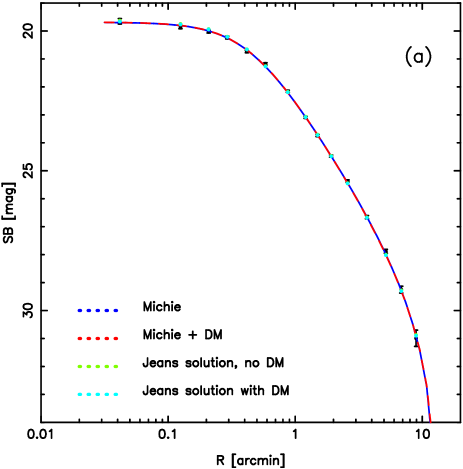
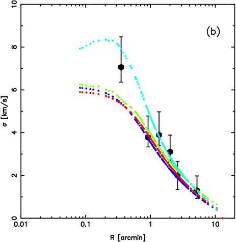
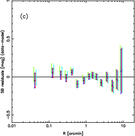
The resulting best fit from 100000 iterations of the lowest temperature chain is shown with the blue line and blue dots in Fig. 1, and is compared to the observational data. The corresponding Michie model parameter values and their uncertainties are listed in Table 1. The solution is fully compatible with the best solutions found in Paper I and Ibata et al. (2011b).
2.2 Jeans equation based models
While the Michie model gives a statistically very good description of the cluster (as we have shown in Paper I), one is nevertheless left wondering how unique this solution is. In that earlier contribution we showed that isotropic Michie models (commonly referred to as King models) cannot account for the observations, but one could attempt at this stage to fit alternative models such as a Plummer, a polytrope or some other model. However, Nature need not follow these simple analytic forms. To attempt to survey the vast space of more general solutions, we have developed an algorithm that takes a different approach: we will assess instead the statistical properties of non-parametric solutions to the Jeans equation.
For a spherically-symmetric system the Jeans equation (Binney & Tremaine, 2008):
| (2) |
relates the cumulative mass inside a radius to the square of the velocity dispersion profiles in the radial () and tangential () directions and to the logarithmic derivatives of and of the density ().
The algorithm we have developed explores these functions from the cluster centre out to the tidal radius. To sample the functions in an economical manner we found it convenient to assign one third of the radial bins to probe the inner region within two core radii with logarithmic bins. Beyond two core radii the remainder of the radial points used linear intervals. We set the value of the central velocity dispersion in the radial direction to be a model parameter. The radial velocity dispersion profile is then defined by the sequence , and the density profile is defined by the sequence , where are the locations of the radial bins. To interpolate these profiles into logarithmic derivatives, we assume that the functions can be approximated locally (between adjacent radial bins) by parabolas in (or ) versus . It is worth noting that it is highly undesirable to define the profiles directly in and , since this requires extremely high accuracy to avoid huge interpolation errors in the logarithmic derivatives. The remaining parameters for the dark matter free case, are the total cluster mass and the stellar mass to light ratio .
Our model therefore has 3 parameters unrelated to the chosen binning (, , ), plus parameters that define the dispersion profile and that define the density profile. We found it convenient to set the number of radial bins to , and certainly with the profiles are smooth and we could reconstruct a Michie model very accurately from artificial data.
The algorithm projects the 3-dimensional functions onto the line of sight, to produce a velocity dispersion profile and a surface brightness profile, from which the model likelihoods are measured using the observed data (Eqn. 1). One further assumption is made in the calculation of the likelihood: we assume that the velocity distributions are Gaussian. This assumption is not necessary for the algorithm to work, and we could have used the velocity moments of the kinematic data directly, or indeed we could have probed other parametrisations of the velocity distribution. However, it is computationally faster and avoids the errors deriving from the calculation of the moments from the data. Furthermore, the assumption is supported by the data: as we showed in Paper I, the observed distribution is consistent with a Gaussian function at all radii probed. The line of sight velocity distributions are then convolved with the uncertainty distribution appropriate for each data point.
We explore this model ( free parameters) using a MCMC scheme444The Bayesian method we are using yields probability distribution functions for the fitting parameters, as well as information on the correlations between these parameters. In this context it is not a problem that we have more fitting parameters than data points.. As before, we use the Parallel Tempering technique with 4 chains to probe progressively more smoothed versions of the likelihood surface. Following Gregory (2005), this is achieved by multiplying by a factor , where is the chain number. The chain corresponds to the lowest “temperature” simulation, which is the one of primary interest.
We implemented an improvement on this method, reducing the dimensionality of the high temperature chains by redefining their radial profiles at only points. Cubic interpolation (in and versus ) between these anchor points was used to fill in intermediate values to maintain 129 radial bins in all chains. Although we attempted a simulation including a chain (i.e. with 9 radial anchor points), it was clear that the interpolation was too crude to be useful.
Some regularisation is required to tell the algorithm that it should avoid exploring very irregular profiles. This was implemented by using a mild smoothing prior on the profiles of the logarithmic derivatives.
An initial simulation with iterations for each chain was run using a Metropolis-Hastings acceptance criterion. As before, all parameters were tuned in lock-step every 1000 iterations, and then refined independently every iterations, so as to ensure an acceptance criterion of 25%. Finally, the 1000 best solutions from this Metropolis-Hastings algorithm were used as inputs for another iteration run using an affine-invariant ensemble sampler algorithm. Our algorithm is based on the “stretch move” algorithm proposed by Goodman & Weare (2010), which we expand to use the above-described multiple “temperature” parallel chains. The simulation uses a population of 1000 “walkers” (which are non-coincident parameter space positions) which evolve from one iteration to the next, and so sample efficiently the likelihood function. The convergence of the method was checked by running simulations from 3 very different starting positions.
While the models built from the distribution function (described in Section 2.1) are consistent by construction, this Jeans-equation based approach can yield solutions that do not have physically possible distribution functions. This is a fundamental drawback of the technique, and cannot be avoided. However, some unphysical models are eliminated by ensuring that the solutions obey the Global Density Slope-Anisotropy Inequality (GDSAI; Ciotti & Morganti, 2010a, b), which is the requirement that at each radius the negative of the logarithmic slope of the stellar density distribution cannot be less than twice the local value of the anisotropy parameter, . We remind the reader that the anisotropy parameter is defined as:
| (3) |
where , and are, respectively, the , and components of the velocity-dispersion tensor. As in Section 2.1, we also impose the requirement that to ensure stability of the resulting models.
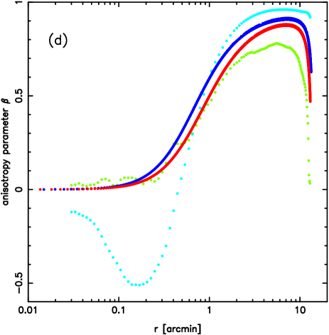
In Fig. 1 we display, in green, the surface brightness profile and velocity dispersion profile of the best solution to the Jeans equation found with this algorithm. The anisotropy profile of this solution is also shown (panel d); it is striking how closely this non-parametric solution matches the behaviour of the best-fit Michie model from Section 2.1 (shown in blue). That our Jeans equation solving algorithm should have selected this model, which is so similar to the previously-fitted Michie model, out of the vast space of possible models, lends strong support to the use of the Michie distribution function to represent the stellar component in this system. The small differences with respect to the Michie model fit in Fig. 1 can be attributed to the differences in the anisotropy profile but the driving factor is the different stellar mass to light ratio ().
3 Models with dark matter
Following the layout of the previous section, we consider first adding dark matter to the Michie model, and then freeing in the Jeans equation so as to also allow for dark matter in those solutions.
3.1 Distribution function based models
We first consider the possibility that the putative dark-matter halo can be described by the double power law density profile (Binney & Tremaine, 2008):
| (4) |
where and are the two power-law indices characterising the shape of the profile, is a scale radius, and is a reference density. In particular, when and we get the Navarro, Frenk, & White (1996, NFW) model; when and we get a profile with a flat inner density distribution, which is very similar to the profile proposed by Burkert (1995). For combinations of and such as those mentioned above the integrated mass of the model diverges at large radii, so it is useful to introduce as an additional parameter a truncation radius such that for . The DM mass contained within a radius is
| (5) |
so the total mass of the DM halo is . If the stellar density distribution is truncated at , the kinematics of the cluster is influenced only by the mass distribution within the stellar tidal radius . It follows that our results are not sensitive to the value of , provided that , which we assume throughout the paper (in other words, our results are not sensitive to the halo concentration ). As a consequence, we define the quantity (the DM mass contained within ), which is more useful than in order to characterise our models. In summary, our model halo is determined by specifying the following four parameters: , , and .
For the DM component, for any choice of the DM profile parameters ( and ) the adimensional potential can be calculated by direct integration of equation (Apendix A) as
In the particular cases of a NFW () and a cored () halo the above integral admits the analytical solutions:
| (6) |
when , and
| (7) |
when .
By incorporating this dark matter potential into the procedure described in §2.1, one can construct spherically symmetric self-consistent stellar systems, truncated at a tidal radius , in equilibrium in the presence of a DM halo (see also Amorisco & Evans, 2011). In these models the parameters , , , , and drive the shape of the density and velocity dispersion profiles, while the values of and determine their normalisation to physical units (see Appendix).
The stellar components of the models considered here are self-consistent by construction, but in principle it is not guaranteed that there is a positive distribution function generating the DM components. For a wide class of two-component models, a necessary condition for consistency is that also the DM component satisfies the GDSAI (Ciotti & Morganti, 2010b). Clearly the specific form of the halo anisotropy profile is not important for the purpose of the present investigation, because the halo influences the observables only through its gravitational potential. However, we impose that in our model the halo density never increases with radius ( at all , i.e. ). This is a necessary condition for consistency only when the halo is isotropic or radially anisotropic, but we impose it as a general constraint because we think it is an astrophysically motivated assumption. However, we noted that it is not excluded that there are self-consistent tangentially biased models with at some .
Even if consistent, some models can be excluded because they are unstable. It has been shown that DM halo has a stabilising effect against the radial-orbit instability (Nipoti, Londrillo, & Ciotti, 2002; Nipoti, Ciotti, & Londrillo, 2011), so at least some models with DM halo are expected to be stable even if they have . However, a full stability analysis of two-component models of NGC 2419 is beyond the purpose of the present paper, so here we conservatively assume as a stability criterion for all the models considered in the present work. With this choice we should effectively exclude unstable models.
We proceed to examine the relative likelihoods of the two-component models built from a power-law dark matter halo and a Michie model stellar component. As in §2.1, we use a “Parallel Tempering” MCMC algorithm with 4 chains to explore the parameter space. The composite model has 9 free parameters: the stellar central density, the Michie model core radius, the anisotropy radius, the central potential, the stellar mass to light ratio, the dark matter central density, the DM characteristic radius and the DM inner and outer power-law indices. For a given set of these 9 parameters, we construct a simulated surface brightness profile and the line of sight velocity distribution as a function of radius, which can be compared directly to the observations.
Several (very weak) priors were imposed on the solutions. The stellar core radius must lie within a factor of 10 of ; the anisotropy radius has to lie between 0.5 and 100 core radii; the central potential parameter has to lie between 2 and 20; and the stellar mass to light ratio is required to stay within the bounds of (i.e. within of the flat region stated above in Section 2.1). Furthermore, we impose that the characteristic radius of the dark matter has to lie between and ; and that the inner and outer power law exponents lie in the ranges and . While certain black hole growth models suggest that the inner power-law slope may be higher than (e.g., Quinlan, Hernquist & Sigurdsson 1995), this is likely to affect only the very central region of the cluster where our data do not constrain the density profile.
Figure 1 shows (in red) the most likely model found by the MCMC algorithm in iterations. The solution has , , a dark matter characteristic radius of , and and . However, we were surprised to find that this model requires very little dark matter: inside of 10′ (the approximate limit of the stellar structure), which is effectively insignificant compared to the stellar mass of . Marginalising over all other parameters, we show the posterior distribution of in Fig. 2; clearly the data appear to favour models without substantial dark matter.
To confirm this curious result, we re-ran the MCMC experiments forcing certain astrophysically-motivated parameter sets: cored DM models () and the NFW model (, ). In an almost identical manner to the more general solution above, the model likelihoods are found to decrease strongly with increasing DM fraction. In an attempt to explore whether the MCMC algorithm was able to escape from solutions with low dark matter, we also performed an experiment forcing a massive DM component, by setting as a strong prior. But again, the distribution of solutions simply clustered near this low mass limit.
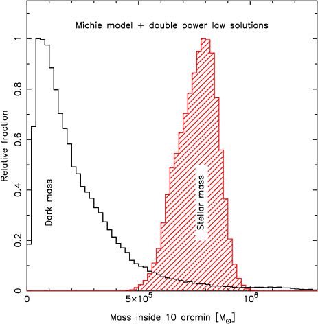
We conclude from this analysis that a simple Michie model where mass traces light is actually preferred by the data over more complicated models that include the possibility of having dark matter in the form of a double power-law profile. The preference for a cored distribution turns out to be very slight - the best models with are only a factor of 1.4 less likely than the best model. However, solutions with some DM seem better than those without DM. This is a manifestation of the tension between stellar and dynamical mass to light ratio that was noted in Bellazzini et al. (2012) (and also in Sollima, Bellazzini & Lee 2012 in other clusters) and which is discussed further below.
3.2 Jeans equation based models
The paucity of dark matter implied by our MCMC survey of the likelihood surface of Michie models is compelling, since the Michie models form a fairly general family of structures, but one is again left wondering to what extent this conclusion depends on the choices of the models selected to examine both the cluster and the dark matter.
For this reason we extended our analysis to a more general set of spherical models where both the dark matter density profile and the stellar density profile are free non-parametric profiles. We reuse the non-parametric MCMC tool described in §2.2 which solves the Jeans equation, finding solutions that are consistent with the data and our priors.

However, given that we now allow for the possibility of dark matter, we require some additional information to close equation 2. To this end we have chosen to free the tangential velocity dispersion profile (in addition to , , , and the profiles of and ). We found it convenient to tabulate this profile as , adding a further parameters to the MCMC fit, plus . The model thus has a total of 389 free parameters.
The MCMC simulations were run in an identical manner to those described in §3.2, using again a hierarchy of 4 different “temperature” chains, each with progressively lower spatial resolution. As before, after initial runs with iterations with a Metropolis-Hastings acceptance algorithm, we switched to using a population of affine-invariant ensemble samplers and reran the simulation for a further iterations.
While the models built from the distribution function (described in Section 3.1) are consistent by construction (at least for as far as the stellar component is concerned), we cannot exclude that some of the two-component models considered are not generated by positive distribution functions. However, as in Section 2.2 we impose at least some necessary conditions for consistency. We additionally imposed the prior that the dark matter density profile decreases with radius and that its logarithmic slope becomes increasingly negative with increasing radius, i.e. if the radial locations and are such that , the logarithmic slopes at these locations obey the condition:
This property is shared by many commonly-used models such as the Plummer sphere, the Michie (and hence King) models, the double power law models if (of which the NFW is a member), among others.

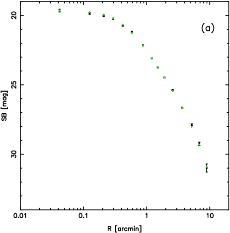
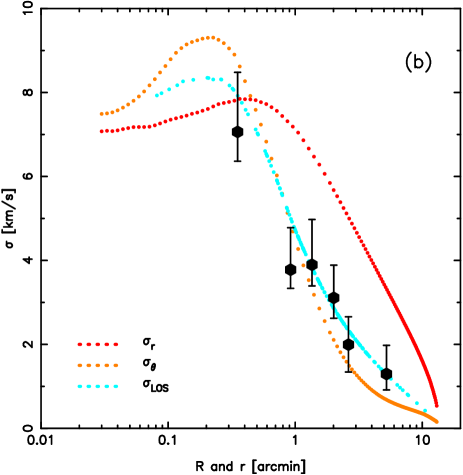
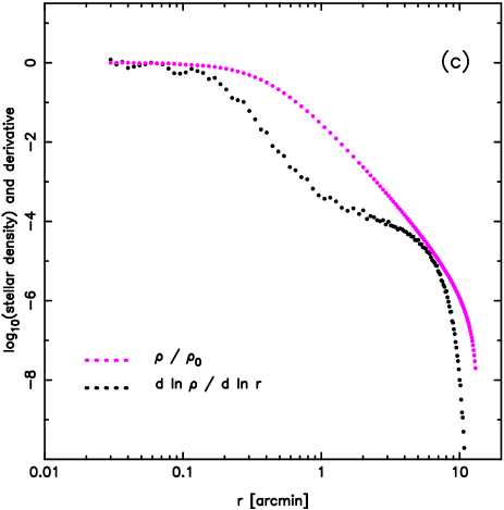
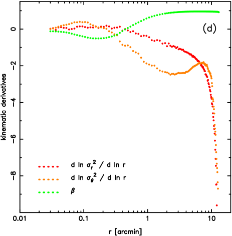
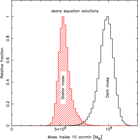
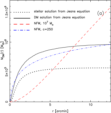
Figure 3 shows the marginalised posterior distribution of the dark matter in the solutions (unshaded histogram). The distribution peaks at , suggesting the presence of a significant dark matter fraction within the central 10′. The posterior distribution of the mass of the stellar component, shown with the hatched histogram, reveals that roughly half the amount in stars as dark matter appears to be present in the solutions. At first sight it would appear that we are facing a simple degeneracy between the total mass of the cluster and the mass to light ratio of the stellar population. This suspicion is reinforced by Figure 4a, which shows the cumulative mass profile in the most likely solution: the dark matter (solid line) and stars (dotted line) follow each other fairly closely (but see also the density profile in panel b). This best solution has a stellar mass to light ratio , within the acceptable range found by Bellazzini et al. (2012). This would therefore suggest that the “dark matter” component is simply the result of the algorithm attempting to force a constant stellar over the whole radial range of the cluster.
However, this option does not appear to be possible, since it would require a profile that is inconsistent with observations and other astrophysical priors, as we show in Figure 5. Here we have calculated the stellar that would be required to account for the total density at a given radius. The constraints on the uniformity of the radial profile of the (Bellazzini et al., 2012), as well as the implausible values beyond make it unlikely that the dark matter component in our Jeans equation solutions are simply due to erroneous assumptions in the profile.
The best Jeans equation solution is displayed in Fig. 6; the panels also illustrate the working of the method by showing the non-parametric profiles that are refined at each Markov-Chain Monte Carlo iteration. As can be seen, the solution gives an almost perfect reproduction of the surface brightness data, and interestingly, is able to fit the full range of the kinematic data, giving a higher (and better) central velocity dispersion than any of the Michie models studied here or in Paper I. Beyond the central , the model is highly radially anisotropic555Recently, Zocchi, Bertin, & Varri (2012) have studied NGC 2419 (among other clusters) using so-called models, which can represent violently relaxed systems. In their analysis (which assumes that no dark matter is present), they also manage to produce a steep central velocity dispersion profile (see their Fig. 3). Note however that their best-fit model has and is quite anisotropic ..
4 Discussion
With current data the answer to the question of whether the globular cluster NGC 2419 contains dark matter or not depends on the model (and hence one’s priors) used to analyse the structure. The choice of using a Michie model for the stars plus a double power law dark matter halo, is appropriate for those who value highly dynamically self-consistent methods and who adhere strongly to cosmological expectations. The most likely solution of this composite model had , which would imply in standard CDM cosmology (following Navarro & Steinmetz 2000) a virial mass of , roughly an order of magnitude lower than the mass of the stellar component in the cluster. The upper 99% confidence limit for the dark mass inside of according to the probability distribution function in Fig. 2 is , and this corresponds to a virial mass of . Such a minuscule halo is some two orders of magnitude lower than expectations for the halo mass of dwarf spheroidal galaxies (Walker, 2012), which have similar stellar content. Thus with this composite model the data prefers virtually no dark matter and one can rule out the possibility that the cluster is embedded at the centre of a dwarf-spheroidal-like mini-halo.
The issue of whether the cluster is located at the centre of the putative DM halo is important for the validity of the analysis presented here. However, the case should in principle be rather similar to that of the globular cluster M54 in the Sagittarius dSph, where the dynamical friction timescale for this similarly-massive globular cluster and its host halo to coincide is estimated to be (Bellazzini et al., 2008). The expectation therefore is that NGC 2419 should reside at the DM halo centre, if it possesses one.
The alternative analysis, using our new Jeans equation solver yields a slightly different answer. The strength of this method is that it does not require one to force a particular analytic functional form on the data. The disadvantage however, is that the resulting models are simply solutions to the Jeans equation, and so many of them are likely to be unphysical (corresponding to a non-physical distribution function) or possibly unstable, but examining the () models individually in the detail necessary to ascertain their validity would be an immense task, far beyond the scope of this contribution.
Nevertheless, taking the distribution in Figure 3 at face value gives a 99% upper bound to the dark matter inside of of , which is somewhat higher than the previous method. The strong difference is that the Jeans equation solution has a 99% lower limit at , effectively demanding more dark matter than stars within . The difference with respect to the DM-free models is that that the solutions are better able to follow the central enhancement of the velocity dispersion. In order to confirm this suspicion, we re-ran the Jeans equation simulations from §3.2 (that include dark matter), this time ignoring the most central 25 radial velocity measurements. The result was a solution very similar to that found in §2.2, with only a small dark matter fraction (mean total dark matter mass of inside of ). This experiment shows that the difference in total dark matter content between the distribution function model solution of §3.1 and the Jeans equation solution of §3.2 is due to the latter attempting to fit better the central velocity dispersion, and that it is those central stars that are driving the requirement for a (small) dark matter fraction. The MCMC algorithm accommodates this mass by changing primarily the anisotropy profile, which can be seen to be negative at in Figure 6d (green dots).
It is interesting to consider which model is preferable: the best composite Michie plus double power-law model, or the best model resulting from the Jeans equation analysis? The traditional frequentist approach is unfortunately not of much use due to the large number of parameters in the Jeans equation solver (we would simply find a negative reduced-, indicating that we have too many parameters). However, answering this question properly with Bayesian evidence is very challenging because the parameters used in the two analysis methods are very different. Indeed, it would require integrating the models over all parameter values, which would be extremely computationally costly, and is beyond the scope of the present work.
In this paper we have used kinematics measurements of NGC 2419 to test the hypothesis that this globular cluster is embedded in a massive DM halo. Another dark component that can in principle be detected via kinematics measurements is a central intermediate mass black hole (Baumgardt, Makino, & Hut, 2005). However, the current kinematic sample does not allow one to set significant constraints on the mass of this putative central black hole, because it affects only the very central () velocity-dispersion profile, which is barely probed by current observations.
4.1 Comparison with previous work
Baumgardt et al. (2009) assume that the putative halo around NGC 2419 has a NFW profile (with ) and use their data to limit the dark mass inside of 500 pc to . Given their model parameters, this corresponds to . In the work of Conroy, Loeb, & Spergel (2011), they also assume that the halo has a NFW profile (with and ) and conclude that , which, for their model parameters, gives a very tight . Our results for the two component models are in reasonable agreement with these previous results. The limits provided above, are more stringent than those of Baumgardt et al. (2009), and unlike Conroy, Loeb, & Spergel (2011), our method does not require the cluster to have suffered strong two-body relaxation, which as we have mentioned, should not have occurred in NGC 2419.
| Michie | Jeans without DM | Michie + DM | Jeans with DM | |
|---|---|---|---|---|
| stellar central density () | (best value) | (best value) | ||
| stellar core radius () | … | … | ||
| anisotropy radius () | … | … | ||
| central potential | … | … | ||
| stellar | ||||
| Stellar mass () | ||||
| Dark mass () | (best value) |
5 Conclusions
We have undertaken an analysis of current data on the kinematics, structure and stellar mass to light ratio of the Galactic globular cluster NGC 2419. This distant halo cluster is a very interesting specimen to study, since it is massive and as such may have been able to maintain a residual dark matter halo over the course of its assimilation into the Milky Way. Thus NGC 2419 allows us to examine the possibility of whether (some) globular clusters formed along with (their now disrupted?) dwarf galaxy hosts within mini dark matter halos.
Our earlier analysis (Paper I) showed that a simple Michie model gives an excellent fit to the state-of-the-art measurements of the kinematics and surface brightness profile of the cluster presented in that contribution. Here we extended that study to investigate whether composite models with an additional dark matter component in the form of a generic double power-law could also be accommodated. To this end we implemented an MCMC parameter search for solutions of this composite system. The Michie distribution function is found to be highly restrictive; while it is as yet not possible to completely rule out the presence of dark matter in NGC 2419, the preferred dark matter fraction is 6% of the stellar mass within 10′ (the approximate limit of the cluster), and there is virtually no room for astrophysically interesting amounts of dark matter that could hint at the formation of clusters within dark matter halos.
In a major effort to assess the model-dependence of these results we developed a new Markov-Chain Monte Carlo algorithm that solves the spherical Jeans equation using non-parametric profiles for the density and velocity dispersion profiles. A very high number of free parameters is required to follow the gradients with sufficient resolution. The code uses a hierarchy of resolutions so as to probe the parameter space as efficiently as possible. These ideas (and the software) should be applicable in the future to analyse other approximately spherical systems of interest, such as dwarf galaxies, elliptical galaxies, or galaxy clusters.
The more general Jeans equation solutions prefer a small dark matter fraction, approximately twice the stellar mass content, and at face value rule out the possibility that there is no dark matter. This last inference depends, however, on the validity of the conclusion by Bellazzini et al. (2012) that the stellar mass to light ratio is invariant with radius. For the most likely solution, the inferred dark matter profile has a very different shape to an NFW model, so it is possible that this putative dark component, if real, is related to unexpected stellar remnants (the expected remnants were taken into account by Bellazzini et al. 2012) rather than cosmological dark matter (note however, that the resolution of present-day simulations that include the relevant baryonic physics do not allow reliable predictions for the profile of dark matter mini-halos of this mass).
In their analysis, Bellazzini et al. (2012) found that assuming a 100% retention of all the dark remnants would have changed the best fit from 1.49 to 1.6. Hence in a standard scenario, changing the fraction of remnant stars will not have a sufficiently large effect to account for Fig. 5. On the other hand, as is pointed out in that contribution, all the currently available (and highly uncertain) models invoked to explain the multiple populations in GCs envisage (a) a progenitor of the present-day cluster with a baryonic mass a factor larger than today, (b) a preferential loss of first generation stars with respect to the second generation, (c) a strong difference in the radial distribution of stars of the two generations (the second one being more concentrated, as is generally observed; see Lardo et al. 2011). This complex star formation history and strong variations in the cluster potential must have occurred in the first of the cluster life. It can be conceived that at this stage both (i) an anomalous production and retention of dark remnants occurred, and (ii) a radial distribution of dark remnants different from that of the light was produced and then remained un-modified in that non-collisional environment.
Therefore if the observed dark matter is of baryonic origin it is likely that it has something to do with the origin and early enrichment of the multiple populations (Cohen, Huang & Kirby, 2011; Mucciarelli et al., 2012) inhabiting NGC2419. On the other hand one may imagine that we see the small remnant of a larger non-baryonic cosmological halo that was nearly completely stripped away from the cluster at early times (see, e.g. Peñarrubia, Navarro & McConnachie 2008). During the first approach to its peri-galacticon, it may have provided the potential well that allowed the cluster to retain ejecta from first generation stars.
Thus all the models we have explored turn out to have very little dark matter in their central regions, and we rule out any connection with mini dark matter halos of the mass that is associated with those in which dwarf galaxies are embedded. This conclusion, though consistent with earlier work on this particularly promising cluster, and consistent also with a large literature on more nearby systems (but which on the whole are clearly not simple isolated systems), remains puzzling. The connection between globular clusters and dwarf galaxy remnants is becoming more and more compelling (Mackey et al., 2010), so it is natural to expect that some clusters retained some of the dark matter of their former host. It is possible that this problem will only be resolved conclusively by obtaining a larger sample of distant halo clusters, but that will require observing further afield in M31, and to be feasible will require the next generation of instruments.
Acknowledgements
R.I. gratefully acknowledges support from the Agence Nationale de la Recherche though the grant POMMME (ANR 09-BLAN-0228). C.N. is supported by the MIUR grant PRIN2008. AS acknowledges the support of INAF through the 2010 postdoctoral fellowship grant. M.B. acknowledges the financial support of INAF through the PRIN-INAF 2009 grant assigned to the project Formation and evolution of massive star clusters, P.I.: R. Gratton.
Apendix A
The distribution function proposed by Michie (1963) has the following phase-space form:
| (8) | |||||
where and are the energy and angular momentum per unit mass, respectively, is the effective potential defined as the difference between the cluster potential (including the contribution of both stars and the dark matter — the latter component will be added in Section 3.1) at a given radius and the potential at the cluster tidal radius (), is a normalization coefficient factor, is a reference velocity dispersion, and are the radial and tangential component of the velocity and is the anisotropy radius: the velocity distribution tends to be isotropic at and radially anisotropic at .
The density and the radial and tangential components of the velocity dispersion can be derived by integrating the above distribution function:
It is convenient to work with the dimensionless quantities
where is the central cluster density and
is the core radius (King 1966). The above equations can be then written as
which can be solved once the potential is known. This last quantity can be written as the sum of the stellar and DM contributions . Both contributions must obey independently the Poisson equation
Here, the subscript refers to either stars or DM. For the stellar component we leave as a free parameter and solve equation (Apendix A) adopting the boundary conditions at the center
Equations (Apendix A) and (Apendix A) can be integrated numerically to derive the three-dimensional density profile, and the radial and tangential velocity dispersion profiles. Finally, the above profiles have been projected on the plane of the sky to obtain the surface mass density
and the line-of-sight velocity dispersion
As described in Section 2.1, the full likelihood analysis performed here requires for each model the knowledge of the distribution of projected velocities (not only its second-order moment). This function can be calculated as
| (11) |
adopting the following change of variables
where .
References
- Amorisco & Evans (2011) Amorisco N. C., Evans N. W., 2011, MNRAS, 411, 2118
- Baumgardt, Makino, & Hut (2005) Baumgardt H., Makino J., Hut P., 2005, ApJ, 620, 238
- Baumgardt & Mieske (2008) Baumgardt H., Mieske S., 2008, MNRAS, 391, 942
- Baumgardt et al. (2009) Baumgardt H., Côté P., Hilker M., Rejkuba M., Mieske S., Djorgovski S. G., Stetson P., 2009, MNRAS, 396, 2051
- Bekki & Yong (2012) Bekki, K., Yong, D., 2012, MNRAS, 419, 2063
- Bellazzini et al. (2012) Bellazzini, M., Dalessandro, E., Sollima, A., Ibata, R., 2012, MNRAS, 423, 844
- Bellazzini et al. (2008) Bellazzini M., Ibata, R., Chapman, S., Mackey, D., Monaco, L., Irwin, M., Martin, N., Lewis, G., Dalessandro, E., 2008, AJ, 136, 1147
- Binney & Mamon (1982) Binney J., Mamon G.A., 1982, MNRAS, 200, 361
- Binney & Tremaine (2008) Binney J., Tremaine S., 2008, Galactic Dynamics 2nd Ed., Princeton University Press, Princeton
- Bradford et al. (2011) Bradford J. D., et al., 2011, ApJ, 743, 167
- Burkert (1995) Burkert A., 1995, ApJ, 447, L25
- Ciotti & Morganti (2010a) Ciotti L., Morganti L., 2010a, MNRAS, 401, 1091
- Ciotti & Morganti (2010b) Ciotti L., Morganti L., 2010b, MNRAS, 408, 1070
- Cohen, Huang & Kirby (2011) Cohen, J., Huang, W., Kirby, E., 2011, ApJ, 740, 60
- Conroy, Loeb, & Spergel (2011) Conroy C., Loeb A., Spergel D., 2011, ApJ, 741, 72
- Dalessandro et al. (2008) Dalessandro, E., Lanzoni, B., Ferraro, F., Vespe, F., Bellazzini, M. Rood, R., 2008, ApJ, 681, 311
- Di Criscienzo et al. (2011) Di Criscienzo M., et al., 2011, AJ, 141, 81
- Fridman & Polyachenko (1984) Fridman A. M., Polyachenko V. L., 1984, Physics of Gravitating Systems. Springer, New York
- Goodman & Weare (2010) Goodman, J., Weare, J., 2010, Comm. App. Math. Comp. Sci., 5, 65
- Gregory (2005) Gregory, P., 2005, Bayesian Logical Data Analysis for the Physical Sciences. Cambridge University Press
- Harris (1996) Harris W. E., 1996, AJ, 112, 1487
- Heggie & Hut (1996) Heggie D. C., Hut P., 1996, IAUS, 174, 303
- Ibata et al. (2011a) Ibata R., Sollima A., Nipoti C., Bellazzini M., Chapman S. C., Dalessandro E., 2011a, ApJ, 738, 186
- Ibata et al. (2011b) Ibata R., Sollima A., Nipoti C., Bellazzini M., Chapman S., Dalessandro E., 2011b, ApJ, 743, 43
- Lardo et al. (2011) Lardo, C., Bellazzini M., Pancino, E., Carretta, E., Bragaglia, A., Dalessandro E., 2011, A&A, 525, 114
- Mackey et al. (2010) Mackey, D., Huxor, A., Ferguson, A., Irwin, M., Tanvir, N., McConnachie, A., Ibata, R., Chapman, S., Lewis, G., 2010, ApJ, 717, 11
- Mapelli et al. (2009) Mapelli M., Ripamonti E., Battaglia G., Tolstoy E., Irwin M. J., Moore B., Sigurdsson S., MNRAS, 396, 1771
- Mashchenko & Sills (2005a) Mashchenko S., Sills A., 2005a, ApJ, 619, 243
- Mashchenko & Sills (2005b) Mashchenko S., Sills A., 2005b, ApJ, 619, 258
- Merritt (1985) Merritt D., 1985, AJ, 90, 1027
- Michie (1963) Michie R. W., 1963, MNRAS, 125, 127
- Milgrom (1983) Milgrom M., 1983, ApJ, 270, 365
- Milgrom (1986) Milgrom M., 1986, ApJ, 306, 9
- Moore (1996) Moore B., 1996, ApJ, 461, L13
- Mucciarelli et al. (2012) Mucciarelli, A., Bellazzini, M., Ibata, R., Merle, T., Chapman, S., Dalessandro, E., Sollima, A., 2012, arXiv:1208.0195
- Navarro & Steinmetz (2000) Navarro J. F., Steinmetz, M., 2000, ApJ, 538, 477
- Navarro, Frenk, & White (1996) Navarro J. F., Frenk C. S., White S. D. M., 1996, ApJ, 462, 563 (NFW)
- Nipoti, Londrillo, & Ciotti (2002) Nipoti C., Londrillo P., Ciotti L., 2002, MNRAS, 332, 901
- Nipoti, Ciotti, & Londrillo (2011) Nipoti C., Ciotti L., Londrillo P., 2011, MNRAS, 414, 3298
- Osipkov (1979) Osipkov L. P., 1979, Soviet Astron. Lett., 5, 42
- Peebles (1984) Peebles P. J. E., 1984, ApJ, 277, 470
- Peñarrubia, Navarro & McConnachie (2008) Peñarrubia, J., Navarro, J., McConnachie, A., 2008, ApJ, 673, 226
- Polyachenko & Shukhman (1981) Polyachenko V. L., Shukhman I. G., 1981, SvA, 25, 533
- Quinlan, Hernquist & Sigurdsson (1995) Quinlan G. D., Hernquist L., Sigurdsson S., 1995, ApJ, 440, 554
- Saitoh et al. (2006) Saitoh T. R., Koda J., Okamoto T., Wada K., Habe A., 2006, ApJ, 640, 22
- Sanders (2012) Sanders, R., 2012, MNRAS, 419, 6
- Sollima, Bellazzini & Lee (2012) Sollima, A., Bellazzini, M., Lee, J.-W., 2012, arXiv:1206.4828
- Walker (2012) Walker, 2012, arXiv:1205.0311
- Zocchi, Bertin, & Varri (2012) Zocchi A., Bertin G., Varri A. L., 2012, A&A, 539, A65