Adaptive numerical integration and control variates for pricing Basket Options

Abstract

We develop a numerical method for pricing multidimensional vanilla options in the Black-Scholes framework. In low dimensions, we improve an adaptive integration algorithm proposed by two of the authors by introducing a new splitting strategy based on a geometrical criterion. In higher dimensions, this new algorithm is used as a control variate after a dimension reduction based on principal component analysis. Numerical tests are performed on the pricing of basket, put on minimum and digital options in dimensions up to ten.

1 Introduction

Pricing financial derivatives generally boils down to numerically compute an expectation, at least for European type contracts. Basically, there are two ways of doing so: either solving a partial differential equation or resorting to Monte Carlo techniques. Monte Carlo integration is known to provide better results when the dimension of the problem increases but for reasonably small dimensional problems, its efficiency is not that clear. However, alternative numerical integration techniques may help in such situations. In the Black-Scholes framework, the pricing of vanilla options reduces to a numerical integration problem over $\mathbb{R}^{d}$, where $d$ is the number of underlying assets. This problem has some specificities coming from the properties of the function to integrate. First, the integrand decreases quickly away from the origin and hence we can consider that the integration domain is a hypercube $[-A,A]^{d}$ with $A$ relatively small. Second, the integrand is clearly not a smooth function in the whole domain as it is only continuous at the interface between the area where the function vanishes and the area where it is positive. Moreover, this interface is neither known and nor located at the boundary of the hypercube so there is no hope of using techniques like the periodisation method [7] to increase the smoothness of the integrand. Finally, the integrand is a muldimensional function in a dimension $d$, which can be large, so one also has to deal with the curse of dimensionality.

Hence, it seems quite natural to use Monte Carlo or quasi-Monte Carlo [17] methods to face such a difficult problem. In fact a crude use of these methods is not necessarily sufficient to reach a good accuracy. Besides the usual variance reduction methods, one needs to develop adaptive methods to make them really competitive. In many situations, the function to integrate or to approximate may have completely different behaviors in terms of variations or even in terms of regularity in different parts of the domain $D.$ In those cases, it might be more efficient to adaptively split $D$ in subregions according to error indicators based on quadrature points. The most famous adaptive Monte Carlo integration routines are MISER [20] and VEGAS [12]. They rely on stratified and importance sampling and error indicators based on the empirical variance, respectively. Quasi-Monte Carlo versions of these two algorithms have been introduced in [21]. More recently, adaptive approaches have been developed for stratified sampling [5, 8] and for importance sampling [11]. The idea of adaptive algorithms is to make use of past simulations to help better leading future ones. In the case of stratified sampling, both the number of samples in each strata and the boundaries of the strata can be learnt inline. The idea remains quite similar for adaptive importance sampling, which consists in adaptively learning the optimal change of measure from the already drawn samples. Following the methodology of [22], two of the authors have developed an adaptive integration algorithm [3] based on quasi-Monte Carlo quadratures, which proved to be efficient for very smooth but also for less smooth functions [16]. This algorithm has already been tested on the pricing of basket options achieving excellent results in dimension two but loosing most of its efficiency for larger dimensions. The loss of accuracy is mainly due to the difficulty to capture the interface between the two regions of interest.

Our goal is to improve this algorithm in order to use it in higher dimensions, for the pricing of more general options like digital or put on minimum options and also for the computations of sensitivities with respect to the parameters of the Black-Scholes model. The improvements of the algorithm will consist in a new splitting criterion and on a dimension reduction using a principal components analysis combined with control variates.

The rest of the paper is organized as follows. In section 2, we describe the different kinds of options considered in the Black-Scholes framework and we discuss the type of sensitivities we are interested in. In section 3, we recall the adaptive algorithm developed in [3] and introduce a new criterion based on very simple geometric considerations like the ones used in mesh refinement for finite element methods. In section 4, we compare the new criterion to the old one on the pricing of different types of options in low dimensions. We focus on examples in dimension two in order to emphasize the quality of the mesh refinement. Section 5 is devoted to sensitivity analysis. We compute the Delta of the different derivatives using standard deterministic techniques like polynomial interpolation allowed by the high accuracy of our adaptive pricing method. The last section deals with higher dimensional models. The adaptive method is coupled with dimension reduction via a principal component analysis to derive a variance reduction method based on control variates.

2 Presentation of the model

2.1 The model framework

We consider a Black-Scholes model in dimension $d$ in which each asset is supposed to follow the standard one dimensional dynamics given under the risk neutral measure by

$$dS_{t}^{i}=S_{t}^{i}(rdt+\sigma_{i}dW_{t}^{i})$$

with $S_{0}^{i}=s^{i}$ and where $W_{t}=(W_{1}^{t},...,W_{d}^{t})$ denotes a vector of correlated standard Brownian motions. The volatility $\sigma$ is a vector in $\mathbb{R}^{d}$, the instantaneous interest rate is $r$ and $(s^{1},...,s^{d})$ is the vector of spot values. The covariance structure of these correlated Brownian motions is supposed to be defined by $\left\langle W,W\right\rangle_{t}=\Gamma t$ where $\Gamma$ is a positive definite matrix with all its diagonal terms equal to one. In the numerical examples considered in the next sections, we assume that

$$\Gamma_{i,j}=\delta_{i,j}+\rho(1-\delta_{i,j})$$

where the parameter $\rho\in]-\frac{1}{d-1},1[$ to ensure that the matrix $\Gamma$ remains positive definite. We introduce the Cholesky decomposition $C$ of $\Gamma$ (such that $CC^{T}=\Gamma)$ and denote by $C_{i}$ its $i^{th}$ row for $1\leq i\leq d$. The Black-Scholes model can be rewritten

$$S_{t}^{i}=S_{0}^{i}\exp\left\{(r-\frac{\sigma_{i}^{2}}{2})t+\sigma_{i}C_{i}B_{t}\right\}$$

where now $B$ is a standard $d-$dimensional Brownian motion.

In this model, we want to price options with payoffs written as functions of the asset price at a maturity time $T$. Hence, the price is given by the discounted expectation $\exp(-rT){\mathbb{E}}(\psi(S_{T}))$ where the function $\psi$ characterizes the option type. In the following, we consider three different multidimensional options for

• Basket options with payoffs

  $$\psi(S_{T})=\left(\sum_{i=1}^{d}\lambda_{i}S_{t}^{i}-K\right)_{+},$$

• Digital basket options with payoffs

  $$\psi(S_{T})=\left(\sum_{i=1}^{d}\lambda_{i}S_{t}^{i}-K\right)_{+}1_{\{\forall\,1\leq i\leq d,\,S_{t}^{i}\leq U_{i}\}},$$

• Put on minimum options with payoffs

  $$\psi(S_{T})=\left(K-\min_{1\leq i\leq d}S_{t}^{i}\right)_{+}.$$

The vector $(\lambda_{1},...,\lambda_{d})$ represents the weight of the different assets within the basket. These weights may be negative to allow to consider exchange options. The variable $K$ denotes the strike price and the vector $U$ corresponds to an upper barrier on the asset price at maturity time $T$. Most of the time, the expectation ${\mathbb{E}}(\psi(S_{T}))$ needs to be computed numerically by means of Monte Carlo methods. In order to use a systematic approach, the expectation ${\mathbb{E}}(\psi(S_{T}))$ is usually rewritten as ${\mathbb{E}}(\phi(G))$ where $G$ is a standard normal random vector in $\mathbb{R}^{d}$ and $\phi:\mathbb{R}^{d}\rightarrow\mathbb{R}^{+}$ is a measurable and integrable function. To use our adaptive method described in the next section, we need to transform the computation of ${\mathbb{E}}(\phi(G))$ into the numerical computation of

$$I(A)=\int_{[-A,A]^{d}}\phi(x)p(x)dx$$

where $p(x)$ is the density of $G$ and $A\in\mathbb{R}_{+}$ is chosen large enough to have a good approximation of ${\mathbb{E}}(\phi(G))$ by $I(A).$

2.2 Key role of the delta

When selling a financial derivative, the price of the option is obviously of a primary interest but one should keep in mind that the original definition of an option price goes back to the replicating theory. The price is actually defined as the value at time $t=0$ of the replicating portfolio. Hence, the price becomes fairly useless if we do not know how to implement the replicating portfolio; hopefully, we precisely know how many stocks the portfolio should carry on at any time $t$ and this quantity is given by the famous Delta of an option defined as the gradient of the option price with respect to the spot vector

$$\Delta=\nabla_{S_{0}}\exp(-rT){\mathbb{E}}(\psi(S_{T})).$$

There are several numerical methods for computing the delta of an option. The most commonly used method is based on a finite difference approach because of its automatic application. However, when coupled with a Monte Carlo method it often yields a poor accuracy unless a very large number of samples is used.

3 Description of the adaptive algorithm

3.1 Quasi-Monte Carlo quadratures

Any adaptive integration method relies on a quadrature rule designed for the non-adaptive case. While Monte Carlo or quasi-Monte Carlo methods can deal with integrands with no or little regularity, usual quadrature rules like Gauss product rules are built for functions having a given regularity or belonging to particular bases. These quadratures should not be too sensitive to the dimensional effect and thus quadrature formulae based on interpolation or approximation on different reduced size bases are considered. In the case of $d-$dimensional Fourier bases on periodic smooth functions, Korobov spaces [9] are built using that the Fourier coefficients $a_{m}$ verify

$$\left|a_{m}\right|\leq\frac{C}{(\widetilde{m_{1}}\widetilde{m_{2}}...\widetilde{m_{Q}})^{\beta}}$$

where $\widetilde{m}=\max(1,\left|m\right|)$ and $\beta>1$ is linked to the regularity of the integrand. The corresponding quadrature formulae are lattice rules [9, 23] which are exact for the most significant Fourier coefficients according to this decay. Non-periodic but smooth functions can be periodized [7] to still use these quadratures but with an increasing constant of decay.

In the case of polynomial approximations, Novak and Ritter [18] have obtained quadrature formulae, which are exact for polynomials with total degree less than a given value. Based on the use of the control variates method on piecewise interpolation polynomials, Atanassov and Dimov [1] built a numerical method reaching an optimal rate of convergence for multivariate smooth functions with a fixed degree of differentiation.

The previous quadratures give highly accurate results for smooth functions but they can yield a really poor accuracy for non-smooth functions. Monte Carlo methods are somehow more stable because they are not sensitive to the smoothness of the integrand. The quadratures developed in [16] combine the approximation on reduced Tchebychef polynomial basis and the use of quasi-Monte Carlo points to build this approximation. They are especially efficient for very smooth functions but they can also handle pretty well only continuous functions. They have been obtained after successive improvements of an initial adaptive Monte Carlo method [13] via quasi-random sequences [15] and the introduction of Tchebychef polynomial basis of Korobov type [14]. We recall these formulae for a multivariate function defined on the hypercube $[-1,1]^{d}$. For $m\in{\mathbb{N}}$, let $\widehat{m}=\max(1,m)$. We introduce the set

$$W_{d,q}=\left\{m\in\mathbb{N}^{d}/\left(\widehat{m_{1}}...\widehat{m_{d}}\right)\leq q\right\}$$

which corresponds to the level $q$ of approximation. The reduced Tchebychef polynomial approximation writes

$$f(x_{1},x_{2},..,x_{d})\simeq\sum_{m\in W_{d,q}}b_{m}T_{m_{1}}(x_{1})T_{m_{2}}(x_{2})..T_{m_{d}}(x_{d})$$

where the $L_{d,q}=card(W_{d,q})$ coefficients $b_{m}$ verify

$$\left|b_{m}\right|\leq\frac{C_{1}}{(\widehat{m_{1}}\widehat{m_{2}}...\widehat{m_{d}})^{2L}}$$

for a $C^{2L}$ function. To compute the numerical approximation of the coefficients $b_{m},$ we fit the model

$$\sum_{m\in W_{d,q}}b_{m}T_{m_{1}}(x_{1})T_{m_{2}}(x_{2})..T_{m_{d}}(x_{d})$$

to the observations of the function $f$ at some quadrature points $P_{i}=(X_{i}^{(1)},...,X_{i}^{(d)})$ with $1\leq i\leq M.$ The choice of the points $P_{i}$ is obviously crucial for the condition number $\kappa(A)$ of the least-square matrix $A$. We have proved in [16] that if these points are independent random variables distributed according to the multidimensional Tchebychef density

$$w(x_{1},x_{2},..,x_{d})=\prod_{i=1}^{d}\frac{1}{\pi\sqrt{1-x_{i}^{2}}}1_{[-1,1]}(x_{i})$$

then $\kappa(A)$ goes to 1 when $M\rightarrow\infty$ at a Monte Carlo speed $\frac{\sigma}{\sqrt{M}}$. Moreover the variance $\sigma^{2}$ is bounded by one for any set $W_{d,q}$. An even better choice to represent the density $w$ is to use quasi-Monte Carlo points or quantization points [19].

We compute numerically the inverse of the matrix $A$ in order to obtain once and for all quadrature formulae for each of the coefficients $b_{m}$ and finally a quadrature formula for the integral itself. In the following, the quadrature points are built using $\alpha\times L_{d,q}$ Halton points with one additional point at each corner of the domain for a total of $M=\alpha\times L_{d,q}+2^{d}$ points. In most situations, the parameter $\alpha$ is chosen equal to $3$ which is sufficient to ensure a small value for $\kappa(A)$. The corner points are control points to detect a possible change of regularity of the function $f$. Nevertheless, we will see in Section 4, that more quadrature points may be necessary to detect this change of regularity on the difficult example of digital options. The approximation of

$$I(f)=\int_{[-1,1]^{d}}f(x)dx$$

is given by the quadrature formula

$$Q_{d,\alpha,q}(f)=\sum_{i=1}^{\alpha\times L_{d,q}+2^{d}}\omega_{i}f(X_{1}^{(i)},...,X_{d}^{(i)})$$

which is obtained thanks to the corresponding approximations $Q_{d,\alpha,q,b_{m}}(f)$ of the coefficients $b_{m}$ and the integration of the approximation model. We also denote by $Q_{d,\alpha,q,R}(f)$ and $Q_{d,\alpha,q,b_{m},R}(f)$ the relative quadrature formulae on a given rectangle $R$ which will be used in the adaptive integration algorithm.

3.2 Error indicators

We keep the same error indicators than the one used in our previous paper [3]. They rely on hierarchical quadratures for the integral of $f$ but also for some of the coefficients of its weighted mean-square approximation. We select two sets $W_{d,q_{1}}$ and $W_{d,q_{2}}$ with $1\leq q_{1}<q_{2}$, the corresponding quadrature formulae $Q_{d,\alpha,q_{1}}(f)$ and $Q_{d,\alpha,q_{2}}(f)$ for the integral of $f$ and also the quadrature formulae for some of the leading coefficients in the approximation model. These coefficients are the $d+1$ coefficients belonging to the set $A_{d}$ of the coefficients $b_{m}$ for which all the indexes $(m_{1},m_{2}..,m_{d})$ are equal to zero or only one is non-zero and equal to one. Our error indicator $E_{d,\alpha,q_{1},q_{2},R}(f)$ is

$$\left|Q_{d,\alpha,q_{1},R}(f)-Q_{d,\alpha,q_{2},R}(f)\right|+\sum_{m/b_{m}\in A_{d}}\left|Q_{d,\alpha,q_{1},b_{m},R}(f)-Q_{d,\alpha,q_{2},b_{m},R}(f)\right|$$

on a given hyperrectangle $R.$ This indicator is more robust than the usual indicator based on the comparison between only $Q_{d,\alpha,q_{1},R}(f)$ and $Q_{d,\alpha,q_{2},R}(f)$. Indeed, it is less likely to happen that all the estimators of the leading coefficients are close to each other but all wrong. The approximate value of the integral on a given hyperrectangle is $Q_{d,\alpha,q_{2},R}(f)$ and the approximate integral of $f$ is the sum of the integrals over all the hyperrectangles.

3.3 Splitting strategies

Now, we describe the splitting strategies used in the numerical experiments. At each step of the algorithm, the list of all the remaining hyper-rectangles involved in the algorithm is stored and these hyperrectangles are sorted according to their error indicator. Once the splitting is performed, the hyperrectangle $R$ with the largest error indicator is removed from the list and the hyperrectangles $R_{1}$ and $R_{2}$ are inserted in the list according to their error indicators $E_{d,\alpha,q_{1},q_{2},R_{1}}(f)$ and $E_{d,\alpha,q_{1},q_{2},R_{2}}(f)$.

3.3.1 Fully adaptive splitting

The first strategy named FAS is fully adaptive. It consists in trying the $d$ possible ways to divide the hyper-rectangle $R$ with largest error indicator in two equal size pieces $R_{1}$ and $R_{2}$ along one of the axes and keeping only the best splitting. The best splitting is the one for which

$$E_{d,\alpha,q_{1},q_{2},R_{1}}(f)+E_{d,\alpha,q_{1},q_{2},R_{2}}(f)$$

is minimum among the $d$ possible choices. Each step of this algorithm requires $dN(\alpha L_{d,q}+2^{d})$ evaluations of the function $f$. The computational cost of the method should also take into account the cost of inserting the two newly created hyperrectangles into the list of all hyperrectangles. This can be done efficiently by an insertion sort which has a complexity of $O(N\log(N))$ for our algorithm with $N$ steps. In most practicals examples, the evaluation of the function $f$ requires a lot of atomic computations and hence it makes sense to neglect the cost the sort compared to the number of function evaluations.

3.3.2 Geometrical Random Splitting

The FAS requires $d$ trials to find the optimal splitting. It is mainly interesting when the integrand has variations different from several degrees of magnitude from one coordinate to another like for instance for the two dimensional function $\cos(200x+y).$ When pricing vanilla options, this kind of situation is unlikely to happen. Furthermore and maybe more importantly, we have noticed in our previous work [3] that the convergence problems of our algorithm came from a too fine splitting in one direction near the interface between the regions where the regularity changes.

We propose another strategy named geometrical random splitting (GRS) in order to reduce the computational costs and to solve the convergence problems by finding more precisely this interface. At each step of the algorithm, we divide the hyperrectangle with the largest error criterion in two equal size pieces $R_{1}$ and $R_{2}$ uniformly at random among the admissible directions. The admissible directions are the ones having the larger length among the axis of the hyperrectangle. The initial hyperrectangle is always a hypercube which means that we can never have a ratio more than two between the different lengths of the axis of the hyperrectangles occurring in the mesh. The cost of the algorithm is $N(\alpha L_{d,q}+2^{d})$ and it is stochastic which enables to compute some statistics on its results.

4 Pricing Vanilla options in low dimensions

In this section, we compare the FAS and the GRS for pricing vanilla options on several examples already treated in [3] and also on examples from the general model. On all numerical examples, the same quadrature formulae will be used for the two methods. The number of iterations of the algorithm will be $N=2000$ for the FAS and consequently $d$ times more for the GRS in order to keep the same complexity.

4.1 Basket options

Let us focus a little on basket options. The price of such options, with payoffs only depending on the asset price at maturity time $T$, can be expressed as an expectation $e^{-rT}{\mathbb{E}}(\psi(S_{T}))$. When the random vector $S_{T}$ has a density $f_{S}$ with respect to the Lebesgue measure, computing this expectation is easily turned into a numerical integration problem

$${\mathbb{E}}(\psi(S_{T}))=\int_{[-\infty,\infty]^{d}}\psi(x)f_{S}(x)dx.$$

When $d=1$, there is no need of a numerical integration as a closed formula exists. In the Black–Scholes framework, we know that

$$S_{T}\stackrel{{\scriptstyle law}}{{=}}\left(S_{0}^{i}\exp\left\{(r-\frac{\sigma_{i}^{2}}{2})T+\sigma_{i}C_{i}\sqrt{T}\;G\right\}\right)_{1\leq i\leq d}$$

where $G$ is a random normal vector with values in ${\mathbb{R}}^{d}$. Hence,

$${\mathbb{E}}(\psi(S_{T}))=\int_{[-\infty,\infty]^{d}}\psi\left(S_{0}^{i}\exp\left\{(r-\frac{\sigma_{i}^{2}}{2})T+\sigma_{i}C_{i}\sqrt{T}\;x\right\},1\leq i\leq d\right)\frac{1}{(2\pi)^{d/2}}e^{-|x|^{2}/2}dx.$$

For the particular case of a call basket option, the payoff $\psi$ writes down

$$\psi(s)=\left(\sum_{i=1}^{d}\lambda_{i}s_{i}-K\right)_{+}.$$

Therefore, if we denote by $V(T,K)$ the price of the call basket option, we can write

$$V(T,K)=e^{-rT}\frac{1}{(2\pi)^{d/2}}\int_{[-\infty,\infty]^{d}}\left(\sum_{i=1}^{d}\lambda_{i}S_{0}^{i}\exp\left\{(r-\frac{\sigma_{i}^{2}}{2})T+\sigma_{i}C_{i}\sqrt{T}\;x\right\}-K\right)_{+}e^{-|x|^{2}/2}dx.$$

Using the equality $(s-K)_{+}-(K-s)_{+}=s-K$ and letting the price of the corresponding put basket option be $U(T,K)=e^{-rT}{\mathbb{E}}\left((K-\sum_{i=1}^{d}\lambda_{i}S_{T}^{i})_{+}\right)$, we obtain the so–called call put parity relationship

$$V(T,K)-U(T,K)=\sum_{i=1}^{d}\lambda_{i}-K\exp(-rT).$$

In general, this formula is used to obtain the hardest price to compute (in terms of variance) between the call or the put option prices from the other. Here, we independently compute the call and put option prices and use this formula as a criterion of accuracy. The infinite integral is truncated and we let

$$V(T,K,A)=e^{-rT}\frac{1}{(2\pi)^{d/2}}\int_{[-A,A]^{d}}\left(\sum_{i=1}^{d}\lambda_{i}S_{0}^{i}\exp\left\{(r-\frac{\sigma_{i}^{2}}{2})T+\sigma_{i}C_{i}\sqrt{T}\;x\right\}-K\right)_{+}e^{-|x|^{2}/2}dx$$

be the truncated estimation of $V(T,K)$. The truncated approximation of the put basket option price $U(T,K,A)$ is defined in a similar way. Note that these multi–dimensional integrals are truncated on a square domain. In all the following examples dealing with basket options, we fix the weights of the basket as $\lambda_{i}=\frac{1}{d}$ so that the baskets are all homogeneous and their weights sum up to one.

4.1.1 Examples in dimension 2

The numerical tests considered in this paragraph are very similar to the ones treated in [2]. Three different values for the strike price are tested, one at the money $K_{1}=100,$ one out $K_{2}=127.80$ and one completely out $K_{3}=300.$ These examples were already studied in [3] and the conclusion was that the FAS was outperforming Monte Carlo and quasi-Monte Carlo integration. Hence, we only compare the GRS to the FAS. Moreover, the new algorithm is only run once as we have a deterministic error criterion based on the call-put parity formula.

The GRS is used with quadrature formulae of degrees $18$ and $24$. The latter corresponds to a number of function evaluations of $2000\times 403\times 2\simeq 1.6\times 10^{6}.$ We give in Tables 1 and 2, the values of the truncated estimations for $A_{1}=12$ and $A_{2}=13$. We also compute

$$C(T,K,A)=\left|V(T,K,A)-U(T,K,A)-\frac{1}{2}S_{0}^{(1)}-\frac{1}{2}S_{0}^{(2)}+K\exp(-rT)\right|$$

for these reference values and denote by $C_{old}(T,K,A)$ the same error indicator using the FAS. Truncating the domain of a real valued standard normal random variable to $[-12,12]$ may seem far too large. This is true from a Monte-Carlo point of view and we have actually also run some tests with more conventional values such as $A=5$. These tests were already showing a far better accuracy than a crude Monte Carlo; the results obtained on the examples of Table 1 already had $4$ accurate digits. However, since we are targeting to compute sensibilities, we need a better accuracy, which explains the choices of the parameter $A$.

	$V$	$U$	$C$	$C_{old}$
$(K_{1},A_{1})$	28.49407706	14.564874729	$2\times 10^{-8}$	$1\times 10^{-8}$
$(K_{1},A_{2})$	28.49407708	14.564874726	$2\times 10^{-10}$	$1\times 10^{-8}$
$(K_{2},A_{1})$	18.85549194	28.853971355	$2\times 10^{-8}$	$2\times 10^{-8}$
$(K_{2},A_{2})$	18.85549196	28.853971353	$2\times 10^{-9}$	$7\times 10^{-9}$
$(K_{3},A_{1})$	1.810536572	160.02292952	$2\times 10^{-8}$	$2\times 10^{-8}$
$(K_{3},A_{2})$	1.810536593	160.02292952	$4\times 10^{-10}$	$4\times 10^{-10}$

Table 1: Basket option with parameters $T=3$, $r=0.05$, $d=2$
$S_{0}^{(1)}=S_{0}^{(2)}=50$, $\sigma_{1}=\sigma_{2}=0.4,\rho=0.3$

On this first example, we obtain a very good accuracy of at least $8$ digits on all the computations of the prices of call and put options. These values are both validated by the parity call put formula and by the comparison between the truncated approximations for the two different values of $A.$ There is no significant difference between the two splitting strategies.

	$V$	$U$	$C$	$C_{old}$
$(K_{1},A_{1})$	20.04091112	6.1117087694	$2\times 10^{-9}$	$1\times 10^{-8}$
$(K_{1},A_{2})$	20.04091112	6.1117087676	$1\times 10^{-10}$	$1\times 10^{-8}$
$(K_{2},A_{1})$	8.915343209	18.913822596	$7\times 10^{-10}$	$2\times 10^{-8}$
$(K_{2},A_{2})$	8.915343211	18.913822598	$5\times 10^{-10}$	$7\times 10^{-9}$
$(K_{3},A_{1})$	0.021755879	158.23414880	$4\times 10^{-10}$	$2\times 10^{-8}$
$(K_{3},A_{2})$	0.021755880	158.23414880	$6\times 10^{-11}$	$4\times 10^{-10}$

Table 2: Basket option with parameters $T=3$, $r=0.05$, $d=2$
$S_{0}^{(1)}=S_{0}^{(2)}=50$, $\sigma_{1}=\sigma_{2}=0.2,\rho=0.7$

The two versions of the algorithm are still very efficient on an example with a smaller volatility and more correlated assets. The accuracy is even better than on the first example and we note that the GRS is now one or two digits more accurate than the FAS.

(a) Geometrical Random Splitting

(b) Fully Adaptive Splitting

Figure 1: Mesh for option of Table 1 with $K=K_{1}=100$

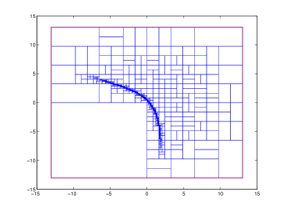
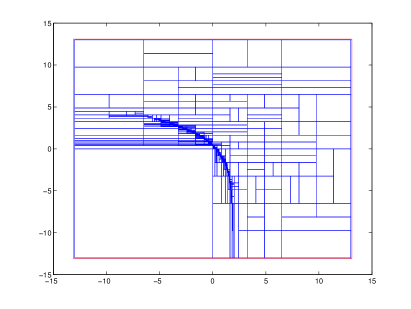
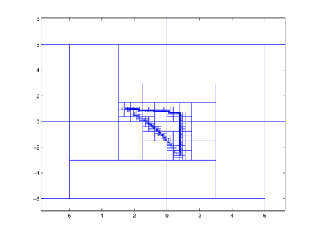
It is also interesting to compare the meshes obtained for the call options for the two splitting strategies. In Figure 1, we plot these meshes for the first example with parameters $(K,A)=(K_{1},A_{2})$. We observe that the refinement is done mainly near the interface separating the region where the function vanishes and the region where it is positive. On these figures, we can see that the GRS is more robust and more able to follow the interface than the FAS.

4.1.2 Examples in dimension $3$ and $4$

In this paragraph, we consider two examples of basket options on independent assets: one example in dimension $3$ and one in dimension $4$. We will run each example with two different strike prices.

We give in Table 3 the values of the truncated estimations for $A_{1}=12$ and $A_{2}=13$ for a $3$ dimensional basket option. The indicator error for this example is based on $E_{3,3,18,24,R}(f)$ and the number of function evaluations is given by $2000\times 1592\times 3\simeq 9.5\times 10^{6}.$

	$V$	$U$	$C$	$C_{old}$
$(K_{1},A_{1})$	14.80805242	2.2717704262	$1\times 10^{-7}$	$4\times 10^{-6}$
$(K_{1},A_{2})$	14.80805257	2.2717705311	$7\times 10^{-8}$	$7\times 10^{-7}$
$(K_{2},A_{1})$	2.927052540	16.212009773	$6\times 10^{-8}$	$8\times 10^{-5}$
$(K_{2},A_{2})$	2.927053375	16.212010568	$2\times 10^{-8}$	$5\times 10^{-5}$

Table 3: $d=3,T=3,r=0.05,\rho=0.3,S_{0}^{(1)}=S_{0}^{(2)}=S_{0}^{(3)}=30\newline \sigma_{1}=\sigma_{2}=\sigma_{3}=0.2$, $K_{1}=90,K_{2}=120$

We observe that the GRS is a lot more accurate than the FAS. The accuracy is about $7$ digits on the at the money option and $8$ on the one out of the money. On the out of the money option, the FAS hardly achieves $5$ digits of accuracy.

We give in Table 4 the values of the truncated estimations for $A_{1}=5$ and $A_{2}=6$. The indicator error for this example is based on $E_{4,3,18,24,R}(f)$ and the number of function evaluations is given by $2000\times 9121\times 4\simeq 4.4\times 10^{7}$.

	$V$	$U$	$C$	$C_{old}$
$(K_{1},A_{1})$	4.22830628	0.32667437	$1\times 10^{-5}$	$3\times 10^{-5}$
$(K_{1},A_{2})$	4.22832492	0.32667871	$1\times 10^{-7}$	$4\times 10^{-4}$
$(K_{2},A_{1})$	0.16841321	5.77905377	$7\times 10^{-6}$	$7\times 10^{-4}$
$(K_{2},A_{2})$	0.16842047	5.77906874	$6\times 10^{-8}$	$6\times 10^{-4}$

Table 4: $d=4,T=1,r=0.05,\rho=0.3,S_{0}^{(1)}=S_{0}^{(2)}=S_{0}^{(3)}=S_{0}^{(4)}=20\newline \sigma_{1}=\sigma_{2}=\sigma_{3}=\sigma_{4}=0.1$, $K_{1}=80,K_{2}=90$

On this last example, the improvement of the algorithm is even more impressive. The accuracy is about $7$ digits with the GRS compared to hardly $4$ with the FAS. The difference between the two values of the criterion $C$ for the two values of $A$ is not due to a wrong computation of the integrals but simply because the integration domain was truncated too much when $A=A_{1}.$

4.2 Put on minimum options

For the pricing of basket options, our approximation criterion was relying on the parity call put formula which does not hold for on minimum or digital options. It required also the pricing of a call and a put to be computed. To define error criteria for general options, we exploit the stochastic nature of the GRS. Instead of running only once this algorithm, we run it ten times only on the call pricing and compute its average $\bar{V}$, its empirical variance $s^{2}_{v}$ and our error criterion will be simply $Err=s_{v}$. We also give the approximation $V_{old}$ obtained with the FAS and the estimation $V_{MC}$ obtained using the crude Monte Carlo method for the computation of the price as the expectation of a normal random vector as described in Section 2.1. This Monte Carlo estimation is accurate up to three digits in relative error and we also give the number of samples required to reach such an accuracy.

4.2.1 Examples in dimension 2

Numerical results are given in Table 5 for both cases $A_{1}=12$ and $A_{2}=15.$

	$\bar{V}$	$V_{old}$	$V_{MC}$	$Err$
Ex1, $A_{1}$	2.10306340730	2.10306339974	2.104291	$1.5\times 10^{-10}$
Ex1, $A_{2}$	2.10306340508	2.10306346643	2.104291	$1.2\times 10^{-10}$
Ex2, $A_{1}$	6.32237986596	6.32237987060	6.325378	$2.2\times 10^{-10}$
Ex2, $A_{2}$	6.32237986541	6.32237985738	6.325378	$1.2\times 10^{-10}$

Table 5: Put on minimum options in dimension $d=2$
Ex1: $T=1,r=0.05,S_{0}^{(1)}=S_{0}^{(2)}=50,\rho=0.1,K=45,\sigma_{1}=\sigma_{2}=0.2$
Ex2: $T=1,r=0.05,S_{0}^{(1)}=S_{0}^{(2)}=50,\rho=0.9,K=55,\sigma_{1}=\sigma_{2}=0.2$

We observe that the GRS provides an estimation of the price which is accurate up to 10 digits. Indeed the integrals for the two values of $A$ are computed with an accuracy of more than 10 digits and they have 10 common digits. The estimations obtained with the FAS are slightly less accurate up to 8 digits.

(a) Geometrical Random Splitting

(b) Fully Adaptive Splitting

Figure 2: Mesh for option of Table 5 with $K=45$ (Ex1)

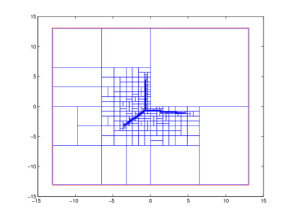
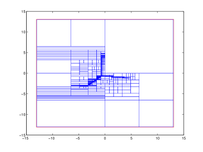
In Figure 2, we plot the two meshes for Ex1 in the case $A=A_{1}.$ We observe on the GRS that the refinement is still done near the interface separating the region where the function vanishes and the region where it is positive but also near a line in the positive part. This additional line is explained by a lack of regularity of the integrand due to the minimum function in its definition. On these two meshes, we can see that once again the GRS is better than the FAS to follow the interfaces where the regularity changes. For both examples, one run of our algorithm requires $1.6\times 10^{6}$ function evaluations meanwhile there are $4.6\times 10^{7}$ and $1.6\times 10^{8}$ Monte Carlo samples for Ex1 and Ex2, respectively. Even if we take into account that 10 runs are used in order to calculate the error indicator, the number of function evaluations for both methods (GRS and crude Monte Carlo) are quite similar. This remains true in the following examples in higher dimensions.

4.2.2 Examples in dimensions 3 and 4

We give in Table 6 the values of the truncated estimations for $A_{1}=12$ and $A_{2}=15$ in dimension 3.

	$\bar{V}$	$V_{old}$	$V_{MC}$	$Err$
Ex3, $A_{1}$	2.89538461	3.021407	2.898180	$6.3\times 10^{-8}$
Ex3, $A_{2}$	2.89538389	2.909697	2.898180	$3.1\times 10^{-8}$
Ex4, $A_{1}$	6.85473710	6.802445	6.854480	$6.3\times 10^{-8}$
Ex4, $A_{2}$	6.85473692	6.795585	6.854480	$6.3\times 10^{-8}$

Table 6: Results for put on minimum options in dimension $d=3$
with $r=0.05$, $S_{0}^{(1)}=S_{0}^{(2)}=S_{0}^{(3)}=50$, $T=1$ and $\sigma_{1}=\sigma_{2}=\sigma_{3}=0.2$.
Ex3: $\rho=0.1,K=45$
Ex4: $\rho=0.9,K=55$

We can see that the GRS is still very efficient and achieves an accuracy of about 7 digits. Now, the FAS gives poorly accurate results and is also clearly less efficient than crude Monte Carlo integration. This confirms the difficulties for the FAS to capture the interface when the dimension of the problem increases. We give in Table 7, the values of the truncated estimations for $A_{1}=12$ and $A_{2}=15$ in dimension 4. The conclusions are the same than in dimension 3. The FAS fails to converge while the GRS is still very accurate. On all examples, whatever the dimension is (up to 4), this latter strategy outperforms the crude Monte Carlo method as we have at least 6 digits of accuracy instead of 3 for a similar complexity.

	$\bar{V}$	$V_{old}$	$V_{MC}$	$Err$
Ex5, $A_{1}$	3.567971	3.560892	3.574086	$6.3\times 10^{-7}$
Ex5, $A_{2}$	3.567971	3.322140	3.574086	$3.1\times 10^{-7}$
Ex6, $A_{1}$	7.212993	6.693007	7.215822	$3.1\times 10^{-7}$
Ex6, $A_{2}$	7.212994	7.305357	7.215822	$3.1\times 10^{-7}$

Table 7: Results on minimum options in dimension $d=4$
with $r=0.05$, $S_{0}^{(1)}=S_{0}^{(2)}=S_{0}^{(3)}=S_{0}^{(4)}=50$, $T=1$ and $\sigma_{1}=\sigma_{2}=\sigma_{3}=\sigma_{4}=0.2$
Ex5: $\rho=0.1,K=45$
Ex6: $\rho=0.9,K=55$

4.3 Digital options

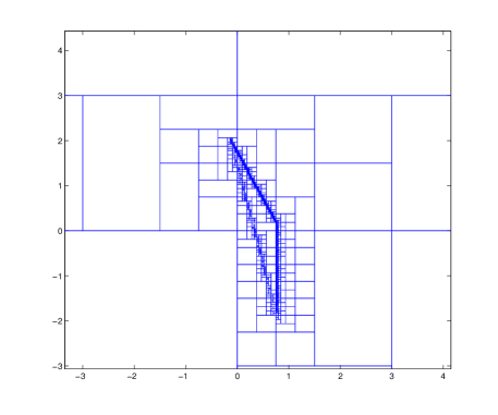
As we will see in the following numerical examples, the pricing of digital options is somehow a much harder problem than the two previous ones. In fact, it is close to the problem of looking for a small subdomain (where the function is positive) somewhere in a large hyperrectangle. This is well illustrated in Figure 4 and even more in Figure 5 where this small subdomain is delimited by three lines. Especially during the first iterations of the algorithm, it may happen that a hyperrectangle of our mesh contains a part of this subdomain but with no quadrature points lying in it. In this case, our error indicator is zero because the function is considered as the null function and consequently this hyperrectangle is never split again. For basket or put on minimum options, we had been able to handle this sampling problem by putting additional quadrature points in each corner of the hyperrectangle. This trick is inefficient in the case of digital options because the subdomain with positive values is small and has a completely different form. In order to solve at least partially these convergence problems, we have increased the parameter $\alpha$ in the number of quadrature points $M=\alpha\times L_{d,q}+2^{d}$ to obtain a larger probability to detect a non-zero value of the function inside the hyperrectangles. Finally, we also compute the median $Med(V)$ of 10 runs of the algorithm because it is a more robust estimator in case of false convergence.

4.3.1 Examples in dimension 2

Our numerical results for both cases $A_{1}=12$ and $A_{2}=15$ are given in Table 8.

	$\bar{V}$	$Med(V)$	$V_{MC}$	$Err$
Ex7, $A_{1}$, $\alpha=3$	2.30072052	2.30072041	2.299709	$3.1\times 10^{-7}$
Ex7, $A_{2}$, $\alpha=3$	2.30071826	2.30071825	2.299709	$3.1\times 10^{-7}$
Ex8, $A_{1}$, $\alpha=3$	0.12540527	0.15675651	0.15600	$6.3\times 10^{-2}$
Ex8, $A_{2}$, $\alpha=3$	0.13848118	0.15675549	0.15600	$2.8\times 10^{-2}$
Ex8, $A_{1}$, $\alpha=15$	0.15693827	0.15693825	0.15600	$3.1\times 10^{-8}$
Ex8, $A_{2}$, $\alpha=15$	0.15681002	0.15675531	0.15600	$9.5\times 10^{-5}$

Table 8: Results for digital call options in dimension $d=2$
with $T=1,r=0.05,S_{0}^{(1)}=S_{0}^{(2)}=50,U_{1}=U_{2}=60,\sigma_{1}=\sigma_{2}=0.2$
Ex7: $\rho=0.1,K=45$
Ex8: $\rho=0.9,K=55$

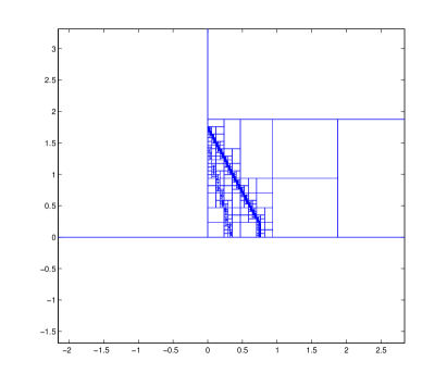
On Ex7, we can see that we have no problem of convergence even with $\alpha=3$. The price is approximately equal to $2.300718$, mean and median are at least 6 digits close in all cases which is confirmed by the error indicator. We also have 3 common digits with the Monte Carlo estimator. The mesh obtained in Figure 3 shows that the subdomain where the function is positive is roughly a small triangle with a surface $\xi$ lower than 8. The ratio $A_{2}^{2}/\xi\simeq 28$ is still small enough to avoid sampling problems.

(a) Geometrical Random Splitting, $A_{1}$

Figure 3: Mesh for option Ex7 of Table 8 $\alpha=3$

(a) Geometrical Random Splitting, $A_{2}$

(b) Geometrical Random Splitting, $A_{1}$

Figure 4: Mesh for option Ex8 of Table 8 $\alpha=3$

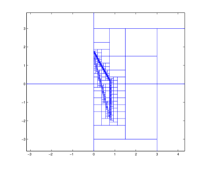
The situation is completely different for Ex8 when $\alpha=3$. Mean and median have no more than 2 common digits, the error indicator is also close to $0.01$. However the median has 3 common digits with the crude Monte Carlo estimator which means that the big convergence problems do not happen so often. We plot in Figure 4 two examples of meshes obtained with $A_{1}$ and $A_{2}$ in situations where the algorithm did not converge. We observe that the refinement is incomplete in both cases and that the one obtained with $A_{2}$ misses half of the region of interest. If we add quadrature points by taking $\alpha=15$, we recover a high accuracy of 7 digits on the integrals at least when $A_{1}=12$. The subdomain we obtain in this case in Figure 5 has now a triangular shape. Its surface is now roughly equal to 1 which explains the convergence problems we encountered when $\alpha=3$ as the ratio $A_{2}^{2}/\xi\simeq 225.$

(a) Geometrical Random Splitting, $A_{1}$

Figure 5: Mesh for option Ex8 of Table 8 $\alpha=15$

For $\alpha=15$, one run of the GRS requires $8\times 10^{6}$ function evaluations, which is 5 times more than in the case $\alpha=3$ meanwhile there are $4.4\times 10^{7}$ and $1.4\times 10^{6}$ Monte Carlo samples for respectively Ex7 and Ex8.

4.3.2 Examples in dimension 3

We give in Table 9, the values of the truncated estimations for $A_{2}=12$ and $A_{2}=15.$

	$\bar{V}$	$Med(V)$	$V_{MC}$	$Err$
Ex9, $\ A_{1}$, $\alpha=20$	1.64950182	1.64950187	1.646800	$2.5\times 10^{-6}$
Ex9, $\ A_{2}$, $\alpha=20$	1.64948232	1.64948236	1.646800	$1.9\times 10^{-6}$
Ex10, $A_{1}$, $\alpha=40$	0.09316076	0.09316072	0.093269	$3.1\times 10^{-7}$
Ex10, $A_{2}$, $\alpha=40$	0.09307638	0.09316133	0.093269	$2.5\times 10^{-4}$

Table 9: Results on digital options in dimension $d=3$
with $r=0.05,T=1,S_{0}^{(1)}=S_{0}^{(2)}=S_{0}^{(3)}=50,U_{1}=U_{2}=U_{3}=60$
Ex9: $\rho=0.1,K=45$
Ex10: $\rho=0.9,K=55$

The number of function evaluations are $6.3\times 10^{7}$ for $\alpha=20$ and $1.3\times 10^{8}$ for $\alpha=40$ meanwhile there are $3.0\times 10^{7}$ and $7.3\times 10^{6}$ Monte Carlo runs respectively for Ex9 and Ex10. On Ex9, we need to increase $\alpha$ to converge up to 5 or 6 digits but the number of function evaluations is still comparable to the size of the Monte Carlo sample. On Ex10 with $A_{2}$, the Monte Carlo method has a smaller variance and the GRS a weaker accuracy which makes these two methods comparable in terms of efficiency. However, with $A_{1}$, the results obtained with the GRS seems very accurate in comparison with those obtained with the Monte Carlo Method. A more detailed discussion about the influence of the initial volume of the hypperrectangle will be given in dimension 4.

4.3.3 Examples in dimension 4

We give in Table 10, the values of the truncated estimations for the usual values $A_{1}=12$, $A_{2}=15$ and also for two smaller values $A_{3}=5$ and $A_{4}=6.$

	$\bar{V}$	$Med(V)$	$V_{MC}$	$Err$
Ex11, $A_{1}$, $\alpha=30$	1.22934667	1.22934613	1.228935	$3.1\times 10^{-6}$
Ex11, $A_{2}$, $\alpha=30$	1.22934272	1.22934341	1.228935	$3.1\times 10^{-6}$
Ex12, $A_{1}$, $\alpha=40$	0.04827239	0.04826375	0.060981	$1.2\times 10^{-2}$
Ex12, $A_{2}$, $\alpha=40$	0.04056702	0.03601258	0.060981	$9.5\times 10^{-3}$
Ex12, $A_{3}$, $\alpha=40$	0.06126412	0.06126407	0.060981	$6.3\times 10^{-7}$
Ex12, $A_{4}$, $\alpha=40$	0.06126593	0.06126569	0.060981	$6.3\times 10^{-7}$

Table 10: Results on digital options for $d=4$
with $r=0.05,T=1,S_{0}^{(1)}=S_{0}^{(2)}=S_{0}^{(3)}=S_{0}^{(4)}=50,U_{1}=U_{2}=U_{3}=U_{4}=60$
Ex11: $\rho=0.1,K=45$
Ex12: $r=0.05,\rho=0.9,K=55$

The number of function evaluations are $4.4\times 10^{8}$ for $\alpha=30$ and $5.8\times 10^{8}$ for $\alpha=40$ meanwhile there are $2.2\times 10^{7}$ and $4.3\times 10^{6}$ Monte Carlo runs respectively for Ex11 and Ex12. Obviously, the complexity of the GRS increases with the dimension but it is still more efficient on Ex11 than the Monte Carlo method. On Ex12, the volume of the subdomain where the function is positive is getting too small compared to the size $A_{2}^{4}$ of the initial hypperrectangle for the GRS to converge. Nevertheless, we have been able to recover a very good accuracy on Ex12 by drastically reducing the size of the initial hypercube using $A_{3}$ and $A_{4}$. Indeed, the corresponding price values have almost 6 common digits and the error criterion is $2\times 10^{-7}.$ This shows that is would be worth using some basic preliminary numerical methods to circumvent the region of interest in a relatively small box.

5 Delta computation

5.1 Tchebychef Interpolation and differentiation

To compute the partial derivatives involved in the computation of the Delta, we use a standard approach based on Tchebychef interpolation polynomials. We describe in detail the two dimensional case for a general function $f(x,y)$. First, we compute the Tchebychef interpolation polynomial $T_{m,h,x_{0},y_{0}}(x)$ of $f(x,y_{0})$ using $m$ interpolation points in the interval $]x-h,x+h[$. The approximation of the first component of the gradient of $f$ at point $(x_{0},y_{0})$ is given by $\displaystyle\frac{\partial}{\partial x}T_{m,h,x_{0},y_{0}}(x)$. Thus, it requires to compute $m$ prices, which is done using the GRS. Using different values of the parameters $h$ and $m$, we are able to obtain reliable Delta approximations.

5.2 Monte Carlo approach

To measure the efficiency of the approach described in Paragraph 5.1, we need an alternative method to compute the Delta, which is sufficiently accurate to serve as a benchmark. We relied on a finite difference approach coupled with a Monte Carlo technique. We closely followed the recommendations of [6] to tune the number of Monte Carlo simulation and the finite difference step accordingly to ensure the best possible accuracy. For a Monte Carlo method with $n$ samples, we used a finite difference step equal to $h_{n}=n^{-1/6}$ so that under mild assumptions the finite difference estimator converges almost surely to the exact value and satisfies a central limit theorem with the rate $n^{-1/3}$.

5.3 Numerical Results

For symmetry reasons, we compute only the first component of the Delta. We compare in table 11 the Monte Carlo approach and the method based on Tchebychef interpolation on 4 examples. These latter are taken in dimension 3 and 4 for basket and minimum options. For the interpolation method, we use two sets of parameters chosen to have two different accurate estimations of the Delta. The maximum number of function evaluations required for the examples in dimension 4 is $5\times 4.4\times 10^{7}=2.2\times 10^{8}$ which is comparable to the number of samples $n$ used in the Monte Carlo method.

	Monte Carlo	$m=3,h=0.05$	$m=5,h=0.1$	$n$
Ex13	0.300088	0.3002853	0.3002864	$1.4\times 10^{8}$
Ex14	-0.240865	-0.2382143	-0.2382098	$1.6\times 10^{8}$
Ex15	0.230224	0.2303219	0.2303214	$1.1\times 10^{8}$
Ex16	-0.186628	-0.1837101	-0.1836998	$1.6\times 10^{8}$

Table 11: Delta Computations with $T=1,r=0.05,\sigma=0.2,S_{0}=50$
Ex13: Basket options, $d=3,\rho=0.1,K=45$
Ex14: Put on minimum options, $d=3,\rho=0.5,K=55$
Ex15: Basket options, $d=4,\rho=0.1,K=45$
Ex16: Put on minimum options, $d=4,\rho=0.5,K=55$

The value of $n$ is chosen to ensure an accuracy of 3 digits on the Delta. All estimations of the Delta using the interpolation method have about 3 common digits with the Monte Carlo estimation. Since for the two sets of parameters we have obtained at least 5 common digits for the two different estimations, we may conclude that the interpolation method is more efficient than the Monte Carlo approach.

6 Dimension reduction and control variates for high dimensional problems

6.1 Description of the method

The GRS developed and tested in the previous sections suffers from the curse of dimensionality but shows a very impressive accuracy in low or medium dimensions up to 4 or 5. In this section, we propose a way to use this method to devise a control variate for high dimensional models. We are still interested in computing expectations of the form ${\mathbb{E}}(\psi(S_{T}))$ where $S_{T}$ is defined as in the previous section. The basic idea of the method is to perform a principal component analysis of $S_{T}$ in order to reduce the dimension of the problem by keeping only the leading components and setting the others to zero. The expectation in the reduced model can be computed quickly and accurately using the GRS and can serve as a control variate for the original problem.

6.1.1 Principal Component Analysis

We rewrite the model to embed the correlation matrix $\Gamma$ into the volatility structure turned into a matrix $\Sigma$ defined by

$$\Sigma=\mathop{\operator@font diag}\nolimits(\sigma_{1},...,\sigma_{d})\;\Gamma\;\mathop{\operator@font diag}\nolimits(\sigma_{1},...,\sigma_{d}).$$

Note that the vector $(\sigma_{1}W_{T},...,\sigma_{2}W_{T})$ is a Gaussian vector with covariance matrix $\sqrt{T}\Sigma$. It is straightforward to check that the matrix $\Sigma$ inherits its symmetric positive definite feature from the one of $\Gamma$ and hence admits an orthonormal basis of eigenvectors with positive eigenvalues. Let $D$ be the diagonal matrix built up with these eigenvalues sorted in decreasing order and let $P$ be the corresponding matrix of eigenvectors sorted accordingly. Note that reordering the columns of $P$ does not change its orthonormal property and that we have $P^{-1}=P^{t}$ and as a consequence $\Sigma=P^{t}DP$. Now, if we let $D^{\frac{1}{2}}=\mathop{\operator@font diag}\nolimits(\sqrt{D_{11}},...,\sqrt{D_{dd}})$ and define the symmetric matrix $H=P^{t}D^{\frac{1}{2}}P$, we obtain $\Sigma=H^{t}H$. This leads to the identity in distribution

$$(\sigma_{1}W_{T},...,\sigma_{2}W_{T})=\sqrt{T}HG$$

where $G$ is a standard normal vector in $\mathbb{R}^{d}.$ Then, we can write the identity in law

$$S_{T}^{i}=S_{0}^{i}\exp\left((r-\frac{\sigma_{i}^{2}}{2})T+\sqrt{T}H_{i}G\right)$$

where $H_{i}$ denotes the $i-{th}$ row of $H.$ This new expression for $S$ can help us to devise a reduced model $\hat{S}$ with effective dimension $l\leq d$ such that $\hat{S}$ can be written

$$\hat{S_{T}^{i}}=S_{0}^{i}\exp\left(r-\frac{\sigma_{i}^{2}}{2})T+\sqrt{T}H_{i}\hat{G}\right)$$

with $\hat{G}=(G_{1},...,G_{l},0,...,0).$

6.1.2 Control variates

If $l$ is sufficiently small, namely less than 3 or 4, we can compute an approximation $\hat{I}$ of ${\mathbb{E}}(\psi(\hat{S_{T}}))$ using the GRS both very accurately and with a small computational cost. If the dimension reduction works well, we can also expect the random variable $\psi(\hat{S_{T}})$ to be close to $\psi(S_{T})$ and as a consequence to appear as a natural choice for a control variate. Our new Monte Carlo estimator for ${\mathbb{E}}(\psi(S_{T}))$ will be

$$\frac{1}{N_{MC}}\sum_{j=1}^{N_{MC}}(\psi(S_{T}^{(j)})-\psi(\hat{S_{T}^{(j)}}))+\hat{I}$$

where the $N_{MC}$ random samples $S_{T}^{(j)}$ and $\hat{S_{T}^{(j)}}$ are built using the same independent drawings $G^{(j)}$ from the standard normal distribution over $\mathbb{R}^{d}.$ Because the effective dimension $l$ of $\hat{G}$ is a lot smaller than $d$ and the GRS is so efficient in low dimensions, one can implement this control variate approach with almost no extra computational cost. The idea of using such a control variate was already proposed for example in [4] but it was limited to a sum of control variates depending on only one variable. Indeed this computation was relying on closed forms for the expectations of the control variates which are only available in dimension one. Hence, our new approach is far more general.

6.2 Numerical results

6.2.1 Toy correlation structures

All the examples deal with basket options in dimension 5 with three different values of the correlation coefficient $\rho$ from very correlated assets ($\rho=0.9$) to negatively correlated assets ($\rho=-0.1$). The different estimations of the price and its confidence interval, named $I_{E_{0}}$, $I_{E_{1}}$, $I_{E_{2}}$, $I_{E_{3}}$, using the control variate method are given in table 12. We compute the estimation of the price $I_{5}$ using the GRS in order to obtain a reference value.

	$I_{E_{0}}$	$I_{E_{1}}$	$I_{E_{2}}$	$I_{E_{3}}$	$I_{5}$
Ex17	$8.61236\pm 0.020$	$8.61333\pm 0.0013$	$8.61357\pm 0.0010$	$8.61407\pm 0.0003$	$8.61404$
Ex18	$7.51683\pm 0.0130$	$7.52217\pm 0.0072$	$7.52395\pm 0.0042$	$7.52621\pm 0.0023$	$7.52490$
Ex19	$7.29012\pm 0.0103$	$7.28436\pm 0.0074$	$7.27969\pm 0.0042$	$7.27931\pm 0.0038$	$7.27548$

Table 12: Basket options with 0.95% confidence interval
$d=5,T=1,r=0.05,K=45,S_{0}=50\newline \sigma=(0.156,0.442,0.325,0.134,0.114)$ and $100,000$ samples
Ex17: $\rho=0.9$, Ex18: $\rho=0.1$, Ex19: $\rho=-0.1$

We observe that the control variate technique gives very good results. Especially with 3 PCA components, the results are very close to $I_{5}$. Moreover, the GRS becoming very costly in dimension 5, the control variate approach with 3 components seems now more efficient.

As it might be expected, we also noticed that when the assets are very correlated the variance reduction is more efficient. With $\rho=0.9$, the first component of the PCA contains almost all the information of the model which ensures a huge variance reduction. When $\rho=-0.1$, even with 3 PCA components, the variance reduction is so small that it hardly compensates the additional cost of the control. Indeed this latter is twice bigger than the initial Monte Carlo cost.

6.2.2 A more general correlation structure

In this paragraph, we are concerned with testing our approach on more realistic covariance structures. We consider a block covariance matrix $G_{Ex20}$, in which the assets can be split into two subsets which are negatively correlated, whereas inside each set all the assets are positively correlated with the same correlation. Such covariance structures are quite common in practice. We can find in Table 13 the results obtained with a standard Monte Carlo and our control variate approach method for different numbers of PCA components. At first sight, one could think that such a covariance structure could cause trouble to our approach and yet it manages to divide the width of the confidence interval by a factor of $10$, which is really impressive if one remembers that to achieve such a confidence interval with a crude Monte Carlo it would require $100$ times more samples. We can see on this example that to effectively reduce the variance, we need at least two PCA components and no closed form formulae are available for basket options in dimension $2$ and $3$. This example highlights the key role played by the GRS approach.

$$\Gamma_{Ex20}=\left(\begin{array}[]{cccccccccc}1&0.8&0.8&0.8&0.8&-0.5&-0.5&-0.5&-0.5&-0.5\\ 0.8&1&0.8&0.8&0.8&-0.5&-0.5&-0.5&-0.5&-0.5\\ 0.8&0.8&1&0.8&0.8&-0.5&-0.5&-0.5&-0.5&-0.5\\ 0.8&0.8&0.8&1&0.8&-0.5&-0.5&-0.5&-0.5&-0.5\\ 0.8&0.8&0.8&0.8&1&-0.5&-0.5&-0.5&-0.5&-0.5\\ -0.5&-0.5&-0.5&-0.5&-0.5&1&0.4&0.4&0.4&0.4\\ -0.5&-0.5&-0.5&-0.5&-0.5&0.4&1&0.4&0.4&0.4\\ -0.5&-0.5&-0.5&-0.5&-0.5&0.4&0.4&1&0.4&0.4\\ -0.5&-0.5&-0.5&-0.5&-0.5&0.4&0.4&0.4&1&0.4\\ -0.5&-0.5&-0.5&-0.5&-0.5&0.4&0.4&0.4&0.4&1\end{array}\right)$$

	$E_{0}$	$E_{1}$	$E_{2}$	$E_{3}$
Ex20	$3.1912\pm 0.011$	$3.1899\pm 0.009$	$3.1908\pm 0.002$	$3.1906\pm 0.001$

Table 13: Prices with 0.95% confidence interval for homogeneous call Basket options on example Ex20 with
$T=2,r=0.02,K=105,\sigma=0.2,S_{0}=100$ and $100,000$ samples

7 Conclusion

In this paper, we have developed a new numerical integration algorithm based on a Geometrical Random Splitting. This new algorithm has been successfully applied to the pricing of Vanilla options in dimensions up to five. In particular, this new algorithm efficiently handles the difficult problems of pricing and hedging digital options. In most situations, the accuracies we have obtained were out of reach for a crude Monte Carlo approach. For higher dimensions, we have shown that the GRS can be used as a control variate when associated to a principal component analysis. The resulting variance reduction was quite impressive especially for very correlated assets. One important issue would be the development of other dimension reduction techniques that could be coupled with the GRS. The GRS itself can obviously have many other applications for instance in computer experiment or in the adaptive approximation of partial differential equations. The GRS algorithm proposed in this paper is very satisfactory on most examples studied.

References

- [1] E. I. ATANASSOV, I. T. DIMOV, A new optimal Monte Carlo method for calculating integral of smooth functions, Monte Carlo Methods and Appl., Vol. 5, No. 2, pp. 149-167, 1999.
- [2] G. DEELSTRA, J. LIINEV, M. VANMAELE, Pricing of arithmetic basket options by conditioning, Insurance: Mathematics and Economics, vol 34, pp. 55-77, 2004.
- [3] C. DE LUIGI, S. MAIRE, Adaptive integration and approximation over hyper-rectangular regions with applications to basket option pricing, Monte Carlo Methods and Applications, 16, (3-4), pp.265-282, 2010.
- [4] S. M. T. EHRLICHMAN and S. G. HENDERSON. Adaptive control variates for pricing multi-dimensional American options, Journal of Computational Finance, 11(1), pp.65–91, 2007.
- [5] P. ETORE, G. FORT, B. JOURDAIN, E. MOULINES, On adaptive stratification, To appear in Annals of operations research.
- [6] P. W. GLYNN, Optimization of stochastic systems via simulation. Proceedings of the 21st conference on Winter simulation, WSC ’89, pages 90–105, New York, NY, USA, 1989. ACM.
- [7] P. HELLUY, S. MAIRE, P. RAVEL, Intégration numérique d’ordre élevé de fonctions régulières ou singulières sur un intervalle, CR. Acad. Sci. Paris, Sér. 1, 327, pp. 843-848, 1998.
- [8] B. JOURDAIN, J. LELONG, Robust adaptive importance sampling for normal random vectors, Annals of applied probability,19 (5), pp. 1687-1718, 2009.
- [9] A. R. KROMMER, C. W. UEBERHUBER. Computational integration. SIAM, 1998.
- [10] D. LAMBERTON, B. LAPEYRE, Introduction to stochastic calculus applied to finance, Chapman & Hall, London, 1996.
- [11] B. LAPEYRE and J. LELONG, A framework for adaptive Monte-Carlo procedures, Monte Carlo Methods Appl., vol. 17 (1), pp.77-98, 2011.
- [12] G. P. LEPAGE, A New Algorithm for Adaptative Multidimensional Integration, Journal of Computational Physics, Vol 27, pp. 192-203, 1978.
- [13] S. MAIRE, Reducing variance using iterated control variates, The Journal of Statistical Computation and Simulation, Vol. 73(1), pp. 1-29, 2003.
- [14] S. MAIRE, An iterative computation of approximations on Korobov-like spaces. Journal of Computational and Applied Mathematics, 157, pp. 261-281, 2003.
- [15] S. MAIRE, Polynomial Approximations of multivariate smooth functions from quasi-random data, Statistics and Computing, 14, pp. 333-336, 2004.
- [16] S. MAIRE, C. DE LUIGI, Quasi-Monte Carlo quadratures for multivariate smooth functions, Applied Numerical Mathematics, 56, no.2, pp. 146-162, 2006.
- [17] H. NIEDERREITER, Quasi-Monte Carlo methods and pseudorandom numbers, Bull. Amer. Math. Soc. 84, pp. 957-1041, 1978.
- [18] E. NOVAK, K. RITTER, High dimensional integration of smooth functions over cubes, Numerishe Mathematik, 75, pp.79-97, 1996.
- [19] G. PAGES, A space vector quantization for numerical Integration, Journal of computational and applied mathematics, 89, pp. 1-38, 1997.
- [20] W. H. PRESS, G. R. FARRAR, Recursive Stratified Sampling for Multidimensional Monte Carlo Integration, Computer in Physics, vol. 4, pp. 190-195, 1990.
- [21] R. SCHURER, Adaptive quasi-Monte Carlo integration based on MISER and VEGAS. Monte Carlo and quasi-Monte Carlo methods 2002, pp. 393-406, Springer, Berlin, 2004.
- [22] R. SCHURER, A comparison between (quasi)-Monte Carlo and cubature rule based methods for solving high-dimensional integration problems, Mathematics and computers in simulation, 62, pp. 509-517, 2003.
- [23] I. H. SLOAN, P. J. KACHOYAN, Lattice methods for multiple integration: Theory, error analysis and examples, SIAM J. Numer. Anal. 24, pp. 116-128, 1987.