Resummation prediction on top quark transverse momentum distribution at large $p_{T}$

Abstract

We study the factorization and resummation of t-channel top quark transverse momentum distribution at large $p_{T}$ in the SM at both the Tevatron and the LHC with soft-collinear effective theory. The cross section in the threshold region can be factorized into a convolution of hard, jet and soft functions. In particular, we first calculate the NLO soft functions for this process, and give a RG improved cross section by evolving the different functions to a common scale. Our results show that the resummation effects increase the NLO results by about $9\%\sim 13\%$ and $4\%\sim 9\%$ when the top quark $p_{T}$ is larger than $50$ and 70 GeV at the Tevatron and the 8 TeV LHC, respectively. Also, we discuss the scale independence of the cross section analytically, and show how to choose the proper scales at which the perturbative expansion can converge fast.

I Introduction

The top quark is the heaviest particle so far discovered, with a mass close to the electroweak symmetry breaking scale, and closely related to various extensions of the standard model (SM). Thus, it provides an effective probe for the electroweak symmetry breaking mechanism and a test for the predictions of the SM through its production or decay.

The production of the single top provides a good opportunity to study the charged weak current interactions of the top quark, e.g., the structure of the $Wtb$ vertex Bernreuther (2008). Besides, it is an important background in many new physics searches at hadron colliders. However, due to the difficulties in discriminating its signature from the large background, it has taken a long time after the discovery of the top quark for the D0 Abazov et al. (2009) and CDF Aaltonen et al. (2009) collaborations at the Tevatron to observe the single top production. Recently, the ATLAS and CMS collaborations at the LHC have also measured the cross section of the single top production at low integrated luminosities Aad et al. (2012); Chatrchyan et al. (2012).

Among the three production modes at hadron colliders, the t-channel is especially important because of its largest cross section at both the Tevatron and the LHC. This process has been extensively studied, including the next-to-leading order (NLO) QCD corrections based on the 2 $\to$ 2 leading order (LO) process, called the five-flavor (5F) scheme Bordes and van Eijk (1995); Stelzer and Willenbrock (1995); Harris et al. (2002); Sullivan (2004); Campbell et al. (2004); Cao and Yuan (2005); Cao et al. (2005); Campbell et al. (2009a). It has been shown that the NLO corrections increase the LO cross section by about $9\%$ and $5\%$ at the Tevatron and LHC, respectively. In Ref. Campbell et al. (2009b), the NLO calculation of the t-channel production based on the 2 $\to$ 3 LO process, called the four-flavor (4F) scheme, was presented, which shows that the inclusive cross section in the 4F scheme is smaller than in the 5F scheme while the uncertainty in the 4F scheme is larger than in 5F scheme. This is due to the fact that in the 5F scheme, the large logarithm of the form log($Q^{2}/m_{b}^{2}$), due to the initial bottom quark, is resummed into the bottom quark parton distribution functions (PDFs) and thus the scale dependence is significantly reduced. Besides, in the 5F scheme, the parton shower Monte Carlo simulation for the t-channel single top production was studied Frixione et al. (2006, 2008); Alioli et al. (2009), and the threshold resummation for this process is carried out with the conventional resummation method  Kidonakis (2006, 2007, 2011), where the partial next-to-next-to-next-to-leading order results are obtained by expanding the resummed cross sections to avoid the infrared singularities and ambiguities from prescription dependence.

In this work, we investigate the resummation of the t-channel single top production in the 5F scheme using soft-collinear effective theory (SCET)  Bauer et al. (2000, 2001); Bauer and Stewart (2001); Bauer et al. (2002); Becher and Neubert (2006a). SCET is developed to describe the behavior of the QCD interactions in collinear and soft regions with the short distance information encoded in the Wilson coefficients. It is very suitable to deal with the scattering processes with multiple scales. In the past ten years, SCET has proved very useful in high energy hard scattering processes. In general, these processes can be divided into two kinds, i.e., the timelike and spacelike. The timelike processes produce a timelike particle in the intermediate or final state, including Drell-Yan production Idilbi and Ji (2005); Idilbi et al. (2005); Becher et al. (2008); Stewart et al. (2010), Higgs boson production Gao et al. (2005); Idilbi et al. (2005); Ahrens et al. (2009a, b); Zhu et al. (2009); Mantry and Petriello (2010), $e^{+}e^{-}$ annihilation to hadrons Lee and Sterman (2007); Fleming et al. (2008a, b); Bauer et al. (2008); Schwartz (2008), color-octet scalar production Idilbi et al. (2009), direct top quark production via FCNC coupling Yang et al. (2006), and s-channel single top production Zhu et al. (2011). The spacelike processes involve a spacelike particle in the intermediate state, such as deep-inelastic scattering Manohar (2003); Chay and Kim (2007); Becher and Neubert (2006a); Chen et al. (2007), direct photon production Becher and Schwartz (2010) and $W$ ($Z$) boson production at large transverse momentum $p_{T}$ Becher et al. (2012). Note that some processes are a mix of these two kinds, e.g., the top quark pair production Ahrens et al. (2010a, b); Beneke et al. (2012).

The threshold region can be easily defined for the timelike processes. It is usually defined as the limit $z=m^{2}/s\to 1$, where $m$ is the invariant mass of the time-like particle and $s$ is the square of the center-of-mass energy. For the spacelike processes, the threshold region is a little more subtle. The threshold region for the deep-inelastic scattering process is given by the Bjorken scaling variable $x\to 1$. For the direct photon production and $W$ ($Z$) boson production at large $p_{T}$, the threshold region is approached when $S_{4}=M^{2}\to 0$, where $M$ is the mass of everything in the final state except the photon ($W$ or $Z$). The t-channel single top production is a spacelike process involving four colored external particles. We define the threshold region as $S_{4}=P_{X}^{2}\to 0$, similar to the case of $W$ or $Z$ production at large $p_{T}$, where $P_{X}^{2}$ represents the mass squared of everything in the final state except the top quark. In this threshold region, the cross section can be factorized as

$$\sigma=H\otimes J\otimes\mathcal{S}\otimes f_{P_{a}}\otimes f_{P_{b}},$$ (1)

where $H,J,\mathcal{S},f_{P}$ are the hard function, jet function, soft function and PDF, respectively. The hard function incorporates the short distance contributions arising from virtual corrections. The jet function describes all collinear interactions inside the outgoing jet. The soft gluon effects coming from all colored particles are contained in the soft function. The PDF denotes the probability of finding a particular parton in the proton.

The final states of the t-channel single top production at hadron colliders consist of a single top quark and a jet at the LO. Additional soft gluons can be emitted from the colored initial and final state particles, and collinear gluons can be emitted in the jet. These contributions are of higher orders in $\alpha_{s}$, but can be large in the threshold region. Besides, the hard part of this process receives a large correction since the usually chosen renormalization scale and the typical transferred momentum are $m_{t}$ and $Q=\sqrt{-\hat{t}}$, respectively, which yield a large logarithm of the form ${\rm ln}(m_{t}^{2}/Q^{2})$. Therefore, it is necessary to resum all of these large logarithm to all orders. In the SCET approach, the different scales in a process can be separated because the soft and collinear degrees are decoupled by the redefinition of the fields Bauer et al. (2002). At each scale, one only needs to deal with the relevant degrees of freedom. In this way, reliable perturbative expansions can be achieved easily, and the dependencies of the final results on the scales are well controlled by the renormalization group (RG) equations. As a result, the singular terms in the hard, jet and soft functions can be resummed conveniently. Furthermore, in numerical calculations, we find that for top quark $p_{T}>$ 50 GeV, the singular terms approximate the fixed-order calculations well, but for $p_{T}<$ 50 GeV, the singular terms do not dominate over the NLO corrections. This is understood because in the larger $p_{T}$ region, the phase space for the additional emitted gluon is more constrained so that the main contribution comes from the soft gluon effects. Thus, we need to know an improved resummation prediction on the top quark transverse momentum distribution in the region of large $p_{T}$, instead of the total cross section. Such a t-channel top quark transverse momentum distribution is actually an observable which can be compared directly with the experimental results , and is an important background in searching for new physics. For example, if there is an extra gauge boson $W^{\prime}$ with a mass around 1 TeV and the standard-model-like couplings, it is better to search this gauge boson in the $t\bar{b}$ final states than the two light jets final states because of the large dijet background from QCD processes. Moreover, one should concentrate on the events with large top quark $p_{T}$ since the top quark from the decay of $W^{\prime}$ usually has a large momentum. In this case, a precise knowledge of the t-channel top quark transverse momentum distribution at large $p_{T}$ in the SM is necessary.

This paper is organized as follows. In Sec. II, we give a brief introduction to SCET. In Sec. III, we analyze the kinematics of the t-channel single top production process and give the definition of the threshold region. In Sec. IV, we present the factorization and resummation formalism for the t-channel single top production in momentum space. In Sec. V, we calculate the hard and soft functions at NLO. Then, we study the scale independence of the final result analytically. In Sec. VI, we discuss the numerical results for t-channel top quark transverse momentum distribution at the Tevatron and the LHC. We conclude in Sec. VII.

II Brief introduction to SCET

To describe collinear fields in SCET, it is convenient to define a lightlike vector $n_{\mu}=(1,\mathbf{n}),\mathbf{n}^{2}=1$. Any four-vector can be light-cone decomposed with respect to $n_{\mu}$ and $\bar{n}_{\mu}=(1,-\mathbf{n})$ as

$$l^{\mu}=l^{-}\frac{n^{\mu}}{2}+l^{+}\frac{\bar{n}^{\mu}}{2}+l^{\mu}_{n\perp},$$ (2)

with $l^{+}=n\!\cdot\!l$ and $l^{-}=\bar{n}\!\cdot\!l$. The momentum of a collinear particle moving along the $n^{\mu}$ direction has the following scaling

$$p^{\mu}=(p^{+},p^{-},p_{n\perp})\sim(\lambda^{2},1,\lambda),$$ (3)

while for a soft particle, the momentum scales as

$$q\sim(\lambda^{2},\lambda^{2},\lambda^{2}),$$ (4)

where $\lambda\ll 1$ is a small expansion parameter in SCET. For example, for an energetic jet with invariant mass $m_{J}$ and energy $E_{J}$, $\lambda=m_{J}/E_{J}$. From the momentum scaling, one can see that the interaction between collinear fields of different directions $n_{i}$ and $n_{j}$ with $n_{i}\cdot n_{j}\gg\lambda^{2}$ will inevitably change the momentum scaling; thus it is forbidden in SCET, but can be included as an external current in our computation. The soft fields, on the other hand, can interact with any collinear field without changing the scaling.

In SCET, the $n$-collinear quark $\psi_{n}$ and gluon field $A_{n}^{\mu}$ can be written as

$$\chi_{n}(x) = W^{\dagger}_{n}(x)\xi_{n}(x),\quad\xi_{n}(x)=\frac{n\!\!\!/\bar{n}\!\!\!/}{4}\psi_{n}(x),$$

$$\mathcal{A}^{\mu}_{n\perp}(x) = \left[W^{\dagger}_{n}iD^{\mu}_{n\perp}W_{n}(x)\right],$$ (5)

where

$$iD^{\mu}_{n\perp}=\mathcal{P}^{\mu}_{n\perp}+g_{s}A^{\mu}_{n\perp}$$ (6)

is the collinear covariant derivative and the label operator $\cal P$ is defined to project out the large momentum component of the collinear field, e.g., ${\cal P}^{\mu}_{n}\xi_{n}=\bar{p}^{\mu}\xi_{n}$. Here we have split $p$ into a sum of large label momentum and small residue momentum,

$$p^{\mu}=\bar{p}^{\mu}+k^{\mu},\qquad\text{with}\qquad\bar{p}^{\mu}=p^{-}\frac{n^{\mu}}{2}+p^{\mu}_{n\perp}.$$ (7)

The $n$-collinear Wilson line,

$$W_{n}(x)=\mathbf{P}\exp\left(ig_{s}\int^{0}_{-\infty}ds\,{\bar{n}}\!\cdot\!A^{a}_{n}(x+s{\bar{n}})t^{a}\right),$$ (8)

which describes the emission of arbitrary $n$-collinear gluons from an $n$-collinear quark or gluon, is constructed to make the collinear fields as defined in Eq. (II) invariant under the collinear gauge transformation. The operator $\mathbf{P}$ is the path-ordered operator acting on the color generator $t^{a}$.

At the LO in $\lambda$, only the $n\!\cdot\!A_{s}$ component of soft gluons can interact with the $n$-collinear field. Such interaction is eikonal and can be removed by a field redefinition Bauer et al. (2002):

$$\chi_{n}(x) \to Y_{n}(x_{-})\chi_{n}(x),$$

$$\mathcal{A}^{\mu}_{n\perp}(x) \to Y_{n}(x_{-})\mathcal{A}^{\mu}_{n\perp}(x)Y^{\dagger}_{n}(x_{-}),$$ (9)

where

$$Y_{n}(x)=\mathbf{P}\exp\left(ig_{s}\int^{0}_{-\infty}ds\,n\!\cdot\!A^{a}_{s}(x+sn)t^{a}\right)$$ (10)

for an incoming Wilson line Bauer et al. (2002); Chay et al. (2005). And for an outgoing Wilson line, it is defined as

$$\tilde{Y}_{n}(x)=\mathbf{P}\exp\left(-ig_{s}\int^{\infty}_{0}ds\,n\!\cdot\!A^{a}_{s}(x+sn)t^{a}\right).$$ (11)

The soft gluon fields are multipole-expanded around $x_{-}$ to maintain a consistent power counting in $\lambda$. For the interaction between the soft gluon fields and massive quark fields, there exists a similar timelike Wilson line Korchemsky and Radyushkin (1992), for example,

$$Y_{v}(x)=\mathbf{P}\exp\left(ig_{s}\int^{0}_{-\infty}ds\,v\!\cdot\!A^{a}_{s}(x+sv)t^{a}\right).$$ (12)

After the field redefinition, the LO SCET Lagrangian is factorized into a sum of different collinear sectors and a soft sector, which do not interact with each other:

$$\mathcal{L}_{\rm SCET}=\sum_{n_{i}}\mathcal{L}^{(0)}_{n_{i}}+\mathcal{L}_{s}+\cdots.$$ (13)

The decoupling of soft gluons from collinear fields is crucial for deriving the factorization formula.

III Analysis of kinematics

In this section, we introduce the relevant kinematical variables needed in our analysis. As an example, we consider the subprocess

$$u(p_{a})+b(p_{a})\to t(q)+X,$$ (14)

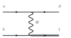
Figure 1: The Feynman diagram for the subprocess $ub\to dt$.

whose Feynman diagram is shown in Fig. 1. First of all, we define two lightlike vectors along the beam directions, $n_{a}$ and $n_{b}$, which are related by $n_{a}=\bar{n}_{b}$. Then we introduce initial collinear fields along $n_{a}$ and $n_{b}$ to describe the collinear particles in the beam directions. In the center-of-mass frame of the hadronic collision, the momenta of the incoming hadrons can be written as

$$P^{\mu}_{a}=E_{\rm CM}\frac{n^{\mu}_{a}}{2},\qquad P^{\mu}_{b}=E_{\rm CM}\frac{n^{\mu}_{b}}{2}.$$ (15)

Here $E_{\rm CM}$ is the center-of-mass energy of the collider and we have neglected the masses of the hadrons. The momenta of the incoming partons, with a light-cone momentum fraction of the hadronic momentum, are

$$p_{a}=x_{a}E_{\rm CM}\frac{n^{\mu}_{a}}{2},\qquad p_{b}=x_{b}E_{\rm CM}\frac{n^{\mu}_{b}}{2}.$$ (16)

At the hadronic and partonic levels, the momentum conservation means

$$P_{a}+P_{b}=q+P_{X},$$ (17)

and

$$p_{a}+p_{b}=q+p_{X},$$ (18)

respectively, where $q$ is the momentum of the top quark. We define the partonic jet with momentum $p_{X}$, which represents the set of all final state partons except the top quark in the partonic processes, while the hadronic jet with momentum $P_{X}$ contains all the hadrons as well as the beam remnants in the final state, except the top quark. Explicitly, $p_{X}=p_{1}+k$, where $p_{1}$ is the momentum of the final state collinear partons forming the jet and $k$ is the momentum of the soft radiations. Such division of momentum is artificial and we have to integrate over the soft momentum to obtain a physical observable.

We also define the Mandelstam variables as

$$s=(P_{a}+P_{b})^{2},\quad u=(P_{a}-q)^{2},\quad t=(P_{b}-q)^{2}$$ (19)

for hadrons, and

$$\hat{s}=(p_{a}+p_{b})^{2},\quad\hat{u}=(p_{a}-q)^{2},\quad\hat{t}=(p_{b}-q)^{2}$$ (20)

for partons, respectively. In terms of the Mandelstam variables, the hadronic and partonic threshold variables are defined as

$$S_{4} \equiv P^{2}_{X}=s+t+u-m^{2}_{t},$$ (21)

$$s_{4} \equiv p^{2}_{X}=\hat{s}+\hat{t}+\hat{u}-m^{2}_{t},$$ (22)

where $m_{t}$ is the mass of top quark. The hadronic threshold limit is defined as $S_{4}\to 0$ Laenen et al. (1998). In this limit, the final state radiations and beam remnants are highly suppressed, which leads to final states consisting of a top quark and a narrow jet, as well as the remaining soft radiations. Taking this limit requires $x_{a}\to 1,\;x_{b}\to 1,\;s_{4}\to 0$ simultaneously. In this limit, we get

$$S_{4} = s_{4}+\hat{s}(\frac{1}{x_{a}x_{b}}-1)+(\hat{t}-m^{2}_{t})(\frac{1}{x_{b}}-1)+(\hat{u}-m^{2}_{t})(\frac{1}{x_{a}}-1)$$ (23)

$$\approx s_{4}+\hat{s}(\bar{x}_{a}+\bar{x}_{b})+(\hat{t}-m^{2}_{t})\bar{x}_{b}+(\hat{u}-m^{2}_{t})\bar{x}_{a}$$

$$\approx s_{4}+(-\hat{t})\bar{x}_{a}+(-\hat{u})\bar{x}_{b},$$

where $\bar{x}_{a,b}=1-x_{a,b}$. This expression can help to check the factorization scale invariance which is shown with more detail in the following. The hadronic threshold enforces the partonic threshold. However, the reverse is not true. The partonic threshold $s_{4}\to 0$ does not forbid a significant amount of beam remnants. We note that in both hadronic and partonic threshold limits, the top quark is not forced to be produced at rest; $i.e.$ it can have a large momentum. For later convenience, we can also write the threshold variable as

$$s_{4}=p^{2}_{X}=(p_{a}+p_{b}-q)^{2}=p^{2}_{1}+2k^{+}E_{1}+{\cal O}(k^{2}),$$ (24)

where $k^{+}=n_{1}\!\cdot\!k$, $k$ is the sum of the momenta of soft radiations; $E_{1}$ is the energy of the quark jet and $n_{1}$ is the lightlike vector associated with the jet direction. In the threshold limit ($s_{4}\to 0$), incomplete cancellation between real and virtual corrections leads to singular distributions $\alpha^{n}_{s}[\ln^{m}(s_{4}/m^{2}_{t})/s_{4}]_{+}$, with $m\leq 2n-1$. It is the purpose of threshold resummation to sum up these contributions to all orders in perturbation theory.

The inclusive total cross section of the t-channel single top production can be written as

$$\sigma = \int dx_{a}\int dx_{b}\int d\hat{t}\int d\hat{u}f_{i/P_{a}}(\mu_{F},x_{a})f_{j/P_{b}}(\mu_{F},x_{b})\frac{1}{2\hat{s}}\frac{d\hat{\sigma}_{ij}}{d\hat{t}d\hat{u}}$$

$$= \int_{0}^{p^{2}_{T,max}}dp_{T}^{2}\int_{-y_{max}}^{y_{max}}dy\int_{x_{b,min}}^{1}dx_{b}\int_{0}^{s_{4}^{max}}ds_{4}\frac{1}{2(x_{b}s+u-m_{t}^{2})}f_{i/P_{a}}(\mu_{F},x_{a})f_{j/P_{b}}(\mu_{F},x_{b})\frac{d\hat{\sigma}_{ij}}{d\hat{t}d\hat{u}},$$

where we have changed the integration variables to be the top quark transverse momentum squared $p^{2}_{T}$, rapidity $y$, $x_{b}$ and $s_{4}$. The regions of the integration variables are limited by

$$p^{2}_{T,max} = \frac{(s-m_{t}^{2})^{2}}{4s},$$

$$y_{max} = \frac{1}{2}{\rm ln}\frac{1+\sqrt{1-sq}}{1-\sqrt{1-sq}},{\rm~{}with~{}}sq=\frac{4s(p_{T}^{2}+m_{t}^{2})}{(s+m_{t}^{2})^{2}},$$

$$x_{b,min} = \frac{-u}{s+t-m_{t}^{2}},$$

$$s_{4}^{max} = x_{b}(s+t-m_{t}^{2})+u,$$ (26)

with

$$t = m_{t}^{2}-\sqrt{s}\sqrt{p_{T}^{2}+m_{t}^{2}}e^{y}$$

$$u = m_{t}^{2}-\sqrt{s}\sqrt{p_{T}^{2}+m_{t}^{2}}e^{-y}.$$ (27)

The other kinematical variables can be expressed in terms of these four integration variables.

IV Factorization and Resummation Formalism

To derive a factorization formula for the t-channel single top production in SCET, we first have to match the full QCD onto the effective theory. In this section, we follow the convention and formalism in Bauer et al. (2009, 2010), where the matching is performed in momentum space. The relevant operator in QCD responsible for the t-channel single top production is

$$O(x)=(\bar{d}\gamma^{\mu}P_{L}u\bar{t}\gamma_{\mu}P_{L}b)(x),$$ (28)

where we have adopted the Feynman gauge for the $W$ boson propagator. This operator contains three massless quarks, which can be described by collinear quarks in SCET, and a massive quark, which can be described by heavy quark effective theory Isgur and Wise (1989). The presence of three different directions and a massive quark is a feature of single top production at hadron colliders. The operator $O(p)$, which is the Fourier transform of $O(x)$, can be written in terms of the momentum-space SCET fields in the threshold region as

$$O(p) = \int\,\frac{d^{4}p_{a}}{(2\pi)^{4}}\frac{d^{4}p_{b}}{(2\pi)^{4}}\frac{d^{4}p_{1}}{(2\pi)^{4}}\frac{d^{4}p_{2}}{(2\pi)^{4}}\frac{d^{4}k_{s}}{(2\pi)^{4}}\mathcal{C}_{I}(p_{a},p_{b};p_{1},p_{2})$$ (29)

$$\times{\cal O}_{in}(p_{a},p_{b}){\cal O}_{out}(p_{1},p_{2}){\cal O}_{S,I}(k_{s})(2\pi)^{4}\delta^{(4)}(p-p_{a}-p_{b}+p_{1}+p_{2}+k_{s}),$$

where the operator ${\cal O}_{in}(p_{a},p_{b})$ is responsible for annihilating the initial u and b quarks with momenta $p_{a}$ and $p_{b}$, respectively, or explicitly,

$${\cal O}^{cd}_{\alpha\beta,in}=\chi^{c}_{\alpha}(p_{a})\chi^{d}_{\beta}(p_{b}),$$ (30)

and ${\cal O}_{out}(p_{1},p_{2})$ is responsible for creating the final d and t quarks with momenta $p_{1}$ and $p_{2}$, respectively, or explicitly,

$${\cal O}^{ef}_{\gamma\delta,out}=\bar{\chi}^{f}_{\delta}(p_{1})\bar{h}^{e}_{\gamma,v}(p_{2}).$$ (31)

Note that we have described the top quark in terms of the heavy quark effective field with a label velocity $v$ Isgur and Wise (1989). Since there are two fermion lines in this process, either of which connects an initial and a final states, we indicate them with the Lorentz ($\alpha,\beta,\gamma,\delta$) and color indices ($c,d,e,f$) explicitly, and retain only quark fields in the operators for simplicity, leaving the other structure in the matching coefficient $\mathcal{C}_{I}$, which is at the LO level

$$\mathcal{C}_{I}^{\delta\alpha,\gamma\beta}=i\frac{g^{2}V_{ud}V_{tb}}{8(\hat{t}-M^{2}_{W})}(\gamma^{\mu}(1-\gamma^{5}))^{\delta\alpha}(\gamma_{\mu}(1-\gamma^{5}))^{\gamma\beta}\delta_{I1}.$$ (32)

Here, the electroweak coupling is defined by $g^{2}=8G_{F}M_{W}^{2}/\sqrt{2}$ where $G_{F}$ is the Fermi constant. $V_{ij}$ is the CKM matrix element and $M_{W}$ is the mass of the $W$ boson. $\delta_{I1}$ denotes the color structure of the t-channel single top production at LO in the singlet-octet basis

$$|c_{1}\rangle=\delta_{fc}\delta_{ed},\qquad|c_{2}\rangle=(t^{a})_{fc}(t^{a})_{ed},$$ (33)

where $t^{a}$ is the generator of the gauge group $SU(3)_{c}$, satisfying

$${\rm tr}[t^{a}t^{b}]=\frac{1}{2}\delta^{ab}.$$ (34)

$I=1$ or $2$ is an index in this color space. In Eq. (29), we can separate the soft gluon field from collinear or massive fields because of the field redefinition in Eq. (II).

The soft operators ${\cal O}_{S,I}$, which are responsible for the soft interactions between different collinear sectors and the top quark, are expressed as

$${\cal O}_{S,1}^{fced}(k_{s}) = \int\,d^{4}xe^{-ik_{s}\,\!\cdot\!\,x}\mathbf{T}\left[\left(\tilde{Y}^{\dagger}_{n_{1}}(x)Y_{n_{a}}(x)\right)^{fc}\left(\tilde{Y}^{\dagger}_{v}(x)Y_{n_{b}}(x)\right)^{ed}\right],$$

$${\cal O}_{S,2}^{fced}(k_{s}) = \int\,d^{4}xe^{-ik_{s}\,\!\cdot\!\,x}\mathbf{T}\left[\left(\tilde{Y}^{\dagger}_{n_{1}}(x)t^{a}Y_{n_{a}}(x)\right)^{fc}\left(\tilde{Y}^{\dagger}_{v}(x)t^{a}Y_{n_{b}}(x)\right)^{ed}\right],$$ (35)

where the time-ordering operator $\mathbf{T}$ is required to ensure the proper ordering of soft gluon fields in the soft Wilson line.

The total cross section for t-channel single top production in the threshold region can be written as

$$\sigma = \frac{1}{2s}\sum_{X}\langle I|O^{\dagger}_{x}(0)|X\rangle\langle X|O_{x}(0)|I\rangle(2\pi)^{4}\delta^{4}(P_{a}+P_{b}-q-P_{X})$$ (36)

$$= \frac{1}{2s}\sum_{X}\int d^{4}x\langle I|O^{\dagger}_{x}(x)|X\rangle\langle X|O_{x}(0)|I\rangle$$

$$= \frac{1}{2s}\sum_{X}\int d^{4}x\int\frac{d^{4}k}{(2\pi)^{4}}e^{-ik\cdot x}\int\frac{d^{4}p}{(2\pi)^{4}}\langle I|O^{\dagger}(k)|X\rangle\langle X|O(p)|I\rangle$$

$$= \frac{1}{2s}\sum_{X}\int\,\frac{d^{4}p}{(2\pi)^{4}}\langle I|O^{\dagger}(0)|X\rangle\langle X|O(p)|I\rangle,$$

where $|I\rangle=|P_{a}P_{b}\rangle$ denotes the initial state protons (antiprotons). Here we distinguish the position space operator from the momentum space one by a subscript $x$. The restriction on the sum over final states $|X\rangle$ is that the final state configuration consists only of a top quark jet whose 3-momentum is in the direction of $\bar{n}_{1}$, a d-quark jet in the direction of $n_{1}$, and soft radiations. This is the configuration that is relevant to threshold resummation and that we are interested in. Under this condition the final state can be written as $|X\rangle=|X_{t}X_{1}X_{s}\rangle$, where $|X_{t}\rangle$, $|X_{1}\rangle$ and $|X_{s}\rangle$ denote the top quark jet, the d-quark jet and the remaining soft radiations, respectively. In the second line of Eq. (36), we have used the momentum conservation delta function to shift the operator $O_{x}^{\dagger}$ to point $x$, and in the third line we have written the operators in momentum space, which are matched onto SCET operators.

Using the notation $\Phi_{2}=\{p_{a},p_{b};p_{1},p_{2}\}$ to express a phase space point Bauer et al. (2009) with $d\Phi_{2}=d^{4}p_{a}d^{4}p_{b}d^{4}p_{1}d^{4}p_{2}/(2\pi)^{16}$ and $\Phi_{2}-k_{s}=p_{a}+p_{b}-p_{1}-p_{2}-k_{s}$, we can write Eq. (36) in a compact form

$$\sigma = \frac{1}{2s}\sum_{X}\int d\Phi^{\prime}_{2}d\Phi_{2}\mathcal{C}^{*}_{J}(\Phi^{\prime}_{2})\mathcal{C}_{I}(\Phi_{2})\int\frac{d^{4}k^{\prime}_{s}}{(2\pi)^{4}}\,\frac{d^{4}k_{s}}{(2\pi)^{4}}(2\pi)^{4}\delta^{(4)}(\Phi_{2}-k_{s})$$ (37)

$$\times\langle I|({\cal O}^{\prime}_{in}{\cal O}^{\prime}_{out}{\cal O}^{\prime}_{S,J})^{\dagger}|X_{t}X_{1}X_{s}\rangle\langle X_{t}X_{1}X_{s}|({\cal O}_{in}{\cal O}_{out}{\cal O}_{S,I})|I\rangle.$$

As we mentioned before, different collinear sectors are decoupled due to field redefinition, and thus the matrix element in Eq. (37) can be factorized into a product of several matrix elements, which obey certain RG equations.

In the following, we further show the matrix elements mentioned above. First, we deal with the top quark sector. Since we have decoupled the soft interaction by field redefinition, the top quark now should be regarded as a noninteracting particle, which can be written as

$$\sum_{X_{t}}\int\frac{d^{4}p^{\prime}_{2}}{(2\pi)^{4}}\frac{d^{4}p_{2}}{(2\pi)^{4}}\langle 0|{h^{e^{\prime}}_{\gamma^{\prime},v^{\prime}}}(p^{\prime}_{2})|X_{t}\rangle\langle X_{t}|\bar{h}^{e}_{\gamma,v}(p_{2})|0\rangle$$ (38)

$$= \int\frac{d^{3}q}{2E_{q}(2\pi)^{3}}({q\!\!\!/}+m_{t})_{\gamma^{\prime}\gamma}\delta^{e^{\prime}e},$$

where summation over the final state $|X_{t}\rangle$ gives rise to a top quark phase space integral. Next, we define the soft function by the soft matrix element as

$$\int dk^{+}S^{d^{\prime}e^{\prime}c^{\prime}f^{\prime}fced}_{JI}(k^{+},\mu) = \frac{1}{N_{c}^{2}}\sum_{X_{s}}\int dk^{+}\frac{d^{4}k^{\prime}_{s}}{(2\pi)^{4}}\frac{d^{4}k_{s}}{(2\pi)^{4}}\langle 0|{\mathcal{O}^{\dagger,d^{\prime}e^{\prime}c^{\prime}f^{\prime}}_{S,J}}(k^{\prime}_{s})|X_{s}\rangle$$ (39)

$$\langle X_{s}|\mathcal{O}^{fced}_{S,I}(k_{s})|0\rangle\delta(k^{+}-n_{1}\!\cdot\!k_{s}),$$

where $N_{c}$ is the number of colors and we have inserted into the above equation an identity operator

$$\mathbf{1}=\int dk^{+}\,\delta[k^{+}-n_{1}\!\cdot\!k_{s}],$$ (40)

because of the constraint from Eq. (24), which expresses the multipole expansion of a soft field interacting with a collinear field Becher and Schwartz (2010). Note that the summation over a final state can be performed $\sum_{X_{s}}|X_{s}(k^{\prime}_{s})\rangle\langle X_{s}(k_{s})|=(2\pi)^{4}\delta^{(4)}(k^{\prime}_{s}-k_{s})$ since there is no restriction in the summation and also there is no explicit dependence of the final states on $|X_{s}\rangle$. Since we are only interested in the cross sections at large top quark $p_{T}$, the final state top quark, jet function and PDFs can be considered to be diagonal in color space. Then we can contract their color indices to obtain the soft function matrix

$$S_{JI}(k^{+},\mu)=\delta^{f^{\prime}f}\delta^{c^{\prime}c}\delta^{e^{\prime}e}\delta^{d^{\prime}d}S^{d^{\prime}e^{\prime}c^{\prime}f^{\prime}fced}_{JI}(k^{+},\mu).$$ (41)

At the LO, it can be written as

$$\mathbf{S}(k^{+},\mu)=\delta(k^{+})\frac{1}{N_{c}^{2}}\left(\begin{array}[]{cc}C_{A}^{2}&0\\ 0&\frac{C_{A}^{2}-1}{4}\end{array}\right),$$ (42)

where $C_{A}$ is the Casimir operator for the adjoint representation of $SU(3)_{c}$. At the NLO, the calculation of the soft function boils down to the evaluation of eikonal diagrams Becher and Schwartz (2010). Since the virtual corrections in SCET vanish, only real emission diagrams are needed to be evaluated. The details of the calculation of these diagrams are given in Appendix A.

For the final state d-quark jet sector, we have

$$\sum_{X_{1}}\int\frac{d^{4}p^{\prime}_{1}}{(2\pi)^{4}}\frac{d^{4}p_{1}}{(2\pi)^{4}}\langle 0|\chi^{f^{\prime}}_{\delta^{\prime}}(p^{\prime}_{1})|X_{1}\rangle\langle X_{1}|\bar{\chi}^{f}_{\delta}(p_{1})|0\rangle$$

$$=\delta^{f^{\prime}f}\int\frac{d^{4}p_{1}}{(2\pi)^{3}}\left(\frac{{n\!\!\!/}_{1}}{2}\right)_{\delta\delta^{\prime}}\theta(p^{0}_{1})\bar{n}_{1}\cdot p_{1}J(p^{2}_{1}),$$ (43)

where the summation over the collinear state has been performed and $J$ is the spin- and color-singlet jet function, defined as

$$\theta(p^{0})\bar{n}_{1}\cdot pJ(p^{2})=\frac{1}{8\pi N_{c}}\int\frac{d^{4}p^{\prime}}{(2\pi)^{4}}{\rm Tr}\langle 0|\bar{n}\!\!\!/_{1}\chi(p^{\prime})\bar{\chi}(p)|0\rangle,$$ (44)

where Tr represents the trace over spin and color indices. At LO, it is just $\delta(p^{2})$. Finally, the initial state $n_{a}$ collinear sector reduces to the conventional PDFs:

$$\int\frac{d^{4}p^{\prime}_{a}}{(2\pi)^{4}}\frac{d^{4}p_{a}}{(2\pi)^{4}}\langle P_{a}|\bar{\chi}^{c^{\prime}}_{\alpha^{\prime}}(p^{\prime}_{a})\chi^{c}_{\alpha}(p_{a})|P_{a}\rangle=\frac{1}{2N_{c}}\delta^{c^{\prime}c}\int^{1}_{0}\frac{dx_{a}}{x_{a}}\left(x_{a}E_{\rm CM}\frac{{n\!\!\!/}_{a}}{2}\right)_{\alpha\alpha^{\prime}}f_{u/P_{a}}(x_{a},\mu)$$ (45)

and similarly for the matrix element for $n_{b}$ direction. Thus the momenta of incoming partons are given by $p_{a(b)}=x_{a(b)}E_{\rm CM}n_{a(b)}/2$.

Combining the above expressions, we obtain (up to power corrections)

$$\sigma = \int dx_{a}dx_{b}d\hat{t}d\hat{u}\frac{1}{2\hat{s}}f_{i/P_{a}}(x_{a},\mu)f_{j/P_{b}}(x_{b},\mu)\frac{d\hat{\sigma}_{ij}^{\rm thres}}{d\hat{t}d\hat{u}},$$ (46)

with

$$\frac{d\hat{\sigma}_{ij}^{\rm thres}}{d\hat{t}d\hat{u}} = \frac{1}{4N^{2}_{c}}\frac{1}{8\pi}\frac{1}{\hat{s}}\lambda_{0,ij}H_{IJ}(\mu)$$ (47)

$$\times\int dk^{+}\int dp_{1}^{2}\,S_{JI}(k^{+},\mu)J(p_{1}^{2},\mu)\delta(s_{4}-p_{1}^{2}-2k^{+}E_{1}),$$

and

$$\lambda_{0,ij}=g^{4}|V_{id}|^{2}|V_{jt}|^{2}\frac{(\hat{s}-m^{2}_{t})\hat{s}}{(\hat{t}-M^{2}_{W})^{2}}.$$ (48)

All the objects in the factorized Eq. (46) have precise field-theoretic definitions so that they can be calculated directly and systematically, except the nonperturbative PDF. The convolution between the jet and soft functions suggests that the partonic threshold consists of two parts. In the case of $s_{4}=0$, there are no collinear or soft gluons emitted. In the small $s_{4}$ region, the number and momentum of collinear and soft gluons are constrained.

At the LO, the hard function $H_{IJ}$ is normalized to $\delta_{I1}\delta_{J1}$. In general, it is related to the amplitudes of the full theory, and is given by Ahrens et al. (2010b)

$$\lambda_{0,ij}H^{(0)}_{IJ} = \frac{1}{\langle c_{I}|c_{I}\rangle\langle c_{J}|c_{J}\rangle}\langle c_{I}|\mathcal{M}^{(0)}_{\rm ren}\rangle\langle\mathcal{M}^{(0)}_{\rm ren}|c_{J}\rangle,$$

$$\lambda_{0,ij}H^{(1)}_{IJ} = \frac{1}{\langle c_{I}|c_{I}\rangle\langle c_{J}|c_{J}\rangle}\left(\langle c_{I}|\mathcal{M}^{(1)}_{\rm ren}\rangle\langle\mathcal{M}^{(0)}_{\rm ren}|c_{J}\rangle+\langle c_{I}|\mathcal{M}^{(0)}_{\rm ren}\rangle\langle\mathcal{M}^{(1)}_{\rm ren}|c_{J}\rangle\right),$$ (49)

where $|\mathcal{M}_{\rm ren}\rangle$ are obtained by subtracting the IR divergences in the $\overline{\rm MS}$ scheme from the UV renormalized amplitudes of the full theory.

Because of the special color structure of this process, the hard function matrix elements do not contribute to the cross section except for $H_{11}$ at the NLO level. In SCET, there is a RG evolution factor connecting the hard scale $\mu_{h}$ and the final common scale $\mu$, which would contain contributions from nondiagonal elements beyond NLO. However, these nondiagonal contributions involve the gluon connecting two fermion lines, resulting in a suppressed color factor $1/N_{c}^{2}$, compared to diagonal ones. Thus, we expect their contributions are small and can be neglected safely. Then the t-channel single top production is considered to be a double deep-inelastic-scattering (DDIS) process Harris et al. (2002). In this case the hard function $H_{11}$ can be further factorized into two parts, i.e., $H_{up}$ and $H_{dn}$, which represent contributions from the up and down fermion lines, respectively, in the Feynman diagram as shown in Fig. 1. This separation is also helpful to make a reliable perturbative prediction for the hard function. The reason is that usually the loop corrections from the up and down fermion lines contain large logarithms of the forms ln$(-\hat{t}/\mu_{h}^{2})$ and ln$((-\hat{t}+m_{t}^{2})/m_{t}/\mu_{h})$, respectively; see Eqs. (51)-(52). It is hard to choose a proper hard scale to make both of them small. In the case of a DDIS process, the two separate hard parts can be evaluated in different scales such that the perturbative expansion is reliable in both parts. As a consequence, we can rewrite Eq. (47) as

$$\frac{d\hat{\sigma}_{ij}^{\rm thres}}{d\hat{t}d\hat{u}} = \frac{1}{4N^{2}_{c}}\frac{1}{8\pi}\frac{1}{\hat{s}}\lambda_{0,ij}H_{up}(\mu)H_{dn}(\mu)$$ (50)

$$\times\int dk^{+}\int dp_{1}^{2}\,\mathcal{S}(k^{+},\mu)J(p_{1}^{2},\mu)\delta(s_{4}-p_{1}^{2}-2k^{+}E_{1}),$$

where $\mathcal{S}(k^{+},\mu)$ denotes the component $S_{11}(k^{+},\mu)$ in Eq. (41).

V The Hard, Jet and Soft Functions at NLO

The hard, jet and soft functions describe interactions at different scales, and they can be calculated order by order in perturbative theory at each scale. At the next-to-next-to-leading logarithmic accuracy, we need the explicit expressions of hard, jet and soft functions up to NLO.

V.1 Hard functions

The hard functions are the absolute value squared of the Wilson coefficients of the operators, which can be obtained by matching the full theory onto SCET. In practice, we need to calculate the one-loop on-shell Feynman diagrams of this process in both the full theory and SCET. In dimensional regularization, the facts that the IR structure of the full theory and the effective theory are identical and that the on-shell integrals are scaleless and vanish in SCET imply that the IR divergence of the full theory is just the negative of the UV divergence of SCET.

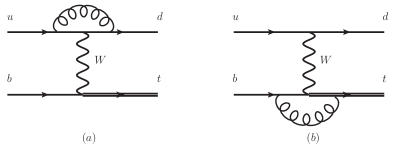
Figure 2: The one-loop Feynman diagrams for the t-channel single top production.

After calculating the one-loop on-shell Feynman diagrams, as shown in Fig. 2, we get the hard functions at NLO as follows:

$$H_{up}(\mu_{h,up}) = 1+\frac{C_{F}\alpha_{s}(\mu_{h,up})}{4\pi}\biggl{(}-2\mathrm{ln}^{2}\frac{-\hat{t}}{\mu_{h,up}^{2}}+6\mathrm{ln}\frac{-\hat{t}}{\mu_{h,up}^{2}}+c^{H,up}_{1}\biggr{)},$$ (51)

$$H_{dn}(\mu_{h,dn}) = 1+\frac{C_{F}\alpha_{s}(\mu_{h,dn})}{4\pi}\biggl{(}-4\mathrm{ln}^{2}\frac{-\hat{t}+m_{t}^{2}}{\mu_{h,dn}m_{t}}+10\mathrm{ln}\frac{-\hat{t}+m_{t}^{2}}{\mu_{h,dn}m_{t}}+c^{H,dn}_{1}\biggr{)},$$ (52)

where

$$c^{H,up}_{1} = -16+\frac{\pi^{2}}{3},$$ (53)

$$c^{H,dn}_{1} = -\frac{2}{\lambda}~{}\mathrm{ln}(1-\lambda)+2\mathrm{ln}^{2}(1-\lambda)+6~{}\mathrm{ln}(1-\lambda)+4\mathrm{Li}_{2}(\lambda)-12-\frac{\pi^{2}}{6}$$ (54)

$$+\frac{2m_{t}^{2}\hat{u}}{\hat{t}(\hat{s}-m_{t}^{2})}\mathrm{ln}\frac{m_{t}^{2}}{m_{t}^{2}-\hat{t}},$$

with $\lambda=\hat{t}/(\hat{t}-m_{t}^{2})$. These results agree with those in Ref. Harris et al. (2002). In order to avoid large logarithms, the natural choices of $\mu_{h,up}$ and $\mu_{h,dn}$ are $\sqrt{-\hat{t}}$ and $(-\hat{t}+m_{t}^{2})/m_{t}$, respectively. The hard functions at the other scales can be obtained by evolution of RG equations. The RG equations for hard functions are governed by the anomalous-dimension matrix, the structure of which has been predicted up to four-loop and two-loop level for the case involving massless Ahrens et al. (2012) and massive partons Becher and Neubert (2009), respectively. In our case, we can write the RG equations for hard functions as

$$\frac{d}{d~{}\mathrm{ln}\mu_{h,up}}H_{up}(\mu_{h,up}) = \biggl{(}2\Gamma_{\rm cusp}~{}\mathrm{ln}\frac{-\hat{t}}{\mu_{h,up}^{2}}+2\gamma_{up}^{V}\biggr{)}H_{up}(\mu_{h,up}),$$ (55)

$$\frac{d}{d~{}\mathrm{ln}\mu_{h,dn}}H_{dn}(\mu_{h,dn}) = \biggl{(}2\Gamma_{\rm cusp}~{}\mathrm{ln}\frac{-\hat{t}+m_{t}^{2}}{\mu_{h,dn}m_{t}}+2\gamma_{dn}^{V}\biggr{)}H_{dn}(\mu_{h,dn}),$$ (56)

where $\Gamma_{\rm cusp}$ is related to the cusp anomalous dimension of Wilson loops with lightlike segments Korchemskaya and Korchemsky (1992), while $\gamma_{up}^{V}$ and $\gamma_{dn}^{V}$ control the single-logarithmic evolution. Their expressions up to two-loop level are shown in Appendix B.

After solving the RG equations, we get the hard functions at an arbitrary scale $\mu$:

$$H_{up}(\mu) = \mathrm{exp}\bigl{[}4S(\mu_{h,up},\mu)-2a_{up}^{V}(\mu_{h,up},\mu)\bigr{]}\bigg{(}\frac{-\hat{t}}{\mu_{h,up}^{2}}\bigg{)}^{-2a_{\Gamma}(\mu_{h,up},\mu)}H_{up}(\mu_{h,up}),$$ (57)

$$H_{dn}(\mu) = \mathrm{exp}\bigl{[}2S(\mu_{h,dn},\mu)-2a_{dn}^{V}(\mu_{h,dn},\mu)\bigr{]}\bigg{(}\frac{-\hat{t}+m_{t}^{2}}{\mu_{h,dn}m_{t}}\bigg{)}^{-2a_{\Gamma}(\mu_{h,dn},\mu)}H_{dn}(\mu_{h,dn}),$$ (58)

where $S(\mu_{h,up},\mu)$ and $a_{up}^{V}$ are defined as Becher et al. (2007)

$$S(\mu_{h,up},\mu) = -\int_{\alpha_{s}(\mu_{h,up})}^{\alpha_{s}(\mu)}d\alpha\frac{\Gamma_{\rm cusp}(\alpha)}{\beta(\alpha)}\int_{\alpha_{s}(\mu_{h,up})}^{\alpha}\frac{d\alpha^{\prime}}{\beta(\alpha^{\prime})},$$ (59)

$$a_{up}^{V}(\mu_{h,up},\mu) = -\int_{\alpha_{s}(\mu_{h,up})}^{\alpha_{s}(\mu)}d\alpha\frac{\gamma_{up}^{V}(\alpha)}{\beta(\alpha)}.$$ (60)

$S(\mu_{h,dn},\mu)$, $a_{\Gamma}$ and $a_{dn}^{V}$ have similar expressions.

V.2 Jet function

The jet function $J(p^{2},\mu)$, defined in Eq. (IV), describes a quark jet of invariant mass squared $p^{2}$. It is process independent and has been calculated at NLO in Manohar (2003) and NNLO in Becher and Neubert (2006b). The RG evolution of the jet function is given by

$$\frac{dJ(p^{2},\mu)}{d\ln\mu}=\left(-2\Gamma_{\rm cusp}\ln\frac{p^{2}}{\mu^{2}}-2\gamma^{J}\right)J(p^{2},\mu)+2\Gamma_{\rm cusp}\int^{p^{2}}_{0}dq^{2}\,\frac{J(p^{2},\mu)-J(q^{2},\mu)}{p^{2}-q^{2}}.$$ (61)

This integro-differential evolution equation can be solved by using the Laplace transformed jet function Becher and Neubert (2006a); Becher et al. (2007):

$$\widetilde{j}(\ln\frac{Q^{2}}{\mu^{2}},\mu)=\int^{\infty}_{0}dp^{2}\,\exp(-\frac{p^{2}}{Q^{2}e^{\gamma_{E}}})J(p^{2},\mu),$$ (62)

which satisfies the the RG equation

$$\frac{d}{d\ln\mu}\widetilde{j}(\ln\frac{Q^{2}}{\mu^{2}},\mu)=\left(-2\Gamma_{\rm cusp}\ln\frac{Q^{2}}{\mu^{2}}-2\gamma^{J}\right)\widetilde{j}(\ln\frac{Q^{2}}{\mu^{2}},\mu).$$ (63)

Then the jet function at an arbitrary scale $\mu$ is given by

$${J}(p^{2},\mu)=\exp\bigl{[}-4S(\mu_{j},\mu)+2a^{J}(\mu_{j},\mu)\bigr{]}\widetilde{j}(\partial_{\eta_{j}},\mu_{j})\frac{1}{p^{2}}\left(\frac{p^{2}}{\mu^{2}_{j}}\right)^{\eta_{j}}\frac{e^{-\gamma_{E}\eta_{j}}}{\Gamma(\eta_{j})},$$ (64)

where $\eta_{j}=2a_{\Gamma}(\mu_{j},\mu)$. The $\mu$-dependent part of the Laplace transformed jet function $\widetilde{j}(L,\mu)$ is determined by the anomalous dimensions of the jet function as in Eq. (63), while the $\mu$-independent part can only be obtained by a fixed-order calculation. At NLO, it is

$$\widetilde{j}(L,\mu) = 1+\frac{\alpha_{s}}{4\pi}\bigg{(}\frac{\Gamma_{0}}{2}L^{2}+\gamma^{J}_{0}L+c^{J}_{1}\bigg{)},$$ (65)

with $c_{1}^{J}=\left(7-\frac{2}{3}\pi^{2}\right)C_{F}$.

V.3 Soft function

The soft function $\mathcal{S}(k^{+},\mu)$, defined in Eq. (39), describes soft interactions between all colored particles. It can be calculated in SCET or in the full theory in the eikonal approximation. The LO soft function is given in Eq. (42). At NLO, we only need to calculate the nonvanishing real emission diagrams in dimensional regularization, as shown in Fig. 3,

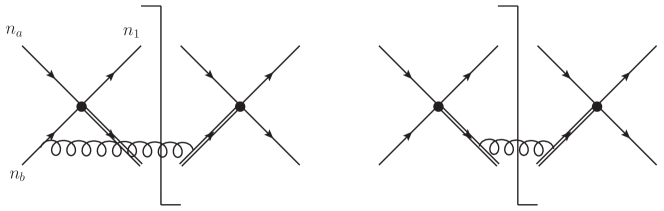
Figure 3: Nonvanishing diagrams contributing to the soft function at NLO. The contributions from the left and right diagrams are denoted as $S^{(1)}_{bt}$ and $S^{(1)}_{tt}$, respectively.

which give

$$S^{(1)}_{bt}(k,\mu) = \frac{2g_{s}^{2}C_{F}\mu^{2\epsilon}}{(2\pi)^{d-1}}\frac{1}{2}\int_{0}^{\infty}\mathrm{d}q^{+}\int_{0}^{\infty}\mathrm{d}q^{-}\int\mathrm{d}^{d-2}q_{\bot}\delta(q^{+}q^{-}-q_{\bot}^{2})\delta(k-n_{1}\cdot q)\frac{n_{b}\cdot v}{(q\cdot n_{b})(q\cdot v)},$$ (66)

and

$$S^{(1)}_{tt}(k,\mu) = \frac{-g_{s}^{2}C_{F}\mu^{2\epsilon}}{(2\pi)^{d-1}}\frac{1}{2}\int_{0}^{\infty}\mathrm{d}q^{+}\int_{0}^{\infty}\mathrm{d}q^{-}\int\mathrm{d}^{d-2}q_{\bot}\delta(q^{+}q^{-}-q_{\bot}^{2})\delta(k-n_{1}\cdot q)\frac{1}{(q\cdot v)^{2}},$$ (67)

respectively. After calculating these integrals by the approach of Ref. Becher and Schwartz (2010), we get

$$S_{bt}^{(1)}(k,\mu) = \frac{2C_{F}\alpha_{s}}{4\pi}\biggl{\{}4\biggl{[}\frac{\ln\frac{k}{\tilde{\mu}}}{k}\biggr{]}_{\star}^{[k,\tilde{\mu}]}+\delta(k)c_{bt}^{S}\biggr{\}},$$

and

$$S_{tt}^{(1)}(k,\mu) = \frac{2C_{F}\alpha_{s}}{4\pi}\biggl{\{}-\biggl{[}\frac{2}{k}\biggr{]}_{\star}^{[k,\tilde{\mu}]}+\delta(k)c_{tt}^{S}\biggr{\}},$$ (68)

respectively, where $\tilde{\mu}=\mu/\sqrt{(2n_{b\bar{b}})/n_{1}^{+2}}=(\mu(-\hat{u})m_{t})/(2(-\hat{t}+m_{t}^{2})E_{1})$. The detail of our calculations and explicit expressions of $c_{bt}^{S}$ and $c_{tt}^{S}$ are given in Appendix A. The star distribution is defined as Schwartz (2008)

$$\left[f(x)\right]_{\star}^{[x,a]} = f(x){\rm~{}for~{}}x>0$$ (69)

$$\int_{0}^{a}dx\left[f(x)\right]_{\star}^{[x,a]}g(x) = \int_{0}^{a}dxf(x)\left[g(x)-g(0)\right].$$ (70)

And the soft function $\mathcal{S}(k,\mu)=S_{bt}(k,\mu)+S_{tt}(k,\mu)$, similar to the jet function, satisfies the RG equation

$$\frac{d}{d\ln\mu}\mathcal{S}(k,\mu)=\biggl{[}-2\Gamma_{\rm cusp}\ln\frac{k}{\tilde{\mu}}+2\gamma^{S}\biggr{]}\mathcal{S}(k,\mu)+2\Gamma_{\rm cusp}\int_{0}^{k}dk^{\prime}\frac{\mathcal{S}(k,\mu)-\mathcal{S}(k^{\prime},\mu)}{k-k^{\prime}}.$$ (71)

The solution to this equation is

$$\mathcal{S}(k,\mu)=\exp\bigl{[}-2S(\mu_{s},\mu)-2a^{S}(\mu_{s},\mu)\bigr{]}\widetilde{s}(\partial_{\eta_{s}},\mu_{s})\frac{1}{k}\biggl{(}\frac{k}{\tilde{\mu}_{s}}\biggr{)}^{\eta_{s}}\frac{e^{-\gamma_{E}\eta_{s}}}{\Gamma(\eta_{s})},$$ (72)

where $\eta_{s}=2a_{\Gamma}(\mu_{s},\mu)$. The Laplace transformed soft function $\widetilde{s}(L,\mu)$ at NLO is given by

$$\widetilde{s}(L,\mu) = 1+\frac{\alpha_{s}}{4\pi}\bigg{(}\Gamma_{0}L^{2}-2\gamma^{S}_{0}L+c^{S}_{1}\bigg{)},$$ (73)

with $c_{1}^{S}=(2c^{S}_{bt}+2c^{S}_{tt}+\frac{2\pi^{2}}{3})C_{F}$.

V.4 Scale independence

In the factorization formalism, we have introduced the hard function, jet function and soft function. Each of them is evaluated at a scale to make the perturbative expansion reliable, and then evolved to a common scale. Therefore, it is important to check the scale independence of the final results. If we expand the exponent in Eq. (57), then we can find that the dependencies on the intermediate scale $\mu_{h,up}$ cancel each other up to $\mathcal{O}(\alpha_{s})$. The same situation happens for $\mu_{h,dn}$ in Eq. (58). The case for the jet scale is more complicated due to the partial derivative operator and the delta function after we use the expansion

$$\frac{1}{p^{2}}\left(\frac{p^{2}}{\mu^{2}_{j}}\right)^{\eta_{j}}=\frac{\delta(p^{2})}{\eta_{j}}+\left[\frac{1}{p^{2}}\right]_{\star}^{[p^{2},\mu_{j}^{2}]}+\eta_{j}\left[\frac{\ln(p^{2}/\mu_{j}^{2})}{p^{2}}\right]_{\star}^{[p^{2},\mu_{j}^{2}]}+\mathcal{O}(\eta_{j}^{2}).$$ (74)

We point out that the scale independence happens for the jet function only in the sense of the integration over $p^{2}$. The case for the soft scale is the same as for the jet scale.

After checking the intermediate scale independence, we discuss the case for the final common scale. Recalling the hadronic threshold definition in Eq. (23) and the cross section near the threshold in Eq. (50), we have

$$\frac{d\sigma}{dS_{4}dy}\propto \int dx_{a}dx_{b}\int dp_{1}^{2}\int dk^{+}\frac{1}{\hat{s}}f_{i/P_{a}}(x_{a},\mu)f_{j/P_{b}}(x_{b},\mu)H_{up}(\mu)H_{dn}(\mu)$$ (75)

$$J(p_{1}^{2},\mu)S(k^{+},\mu)\delta(S_{4}-(-\hat{t})(1-x_{a})-(-\hat{u})(1-x_{b})-p_{1}^{2}-2k^{+}E_{1}),$$

where we have changed the integration variables $d\hat{t}d\hat{u}$ to $dp_{T}^{2}dy$ and then to $dS_{4}dy$. From this equation, we can see clearly the connection between the threshold region of the whole system, represented by $S_{4}$, and those of the parts of the system, represented by $(1-x_{a}),(1-x_{b}),p_{1}^{2}$ and $k^{+}$, respectively. To change the convolution form to a simpler product form, we apply the Laplace transformation to the above equation and obtain

$$\frac{d\tilde{\sigma}}{dQ^{2}dy}=\int_{0}^{\infty}dS_{4}\exp\left(-\frac{S_{4}}{Q^{2}e^{\gamma_{E}}}\right)\frac{d\sigma}{dS_{4}dy}.$$ (76)

The Laplace transformed jet function and its RG evolution are given in Eq. (62) and Eq. (63). Here, for convenience, we write its RG equation again as

$$\frac{d}{d\ln\mu}\widetilde{j}(\ln\frac{Q^{2}}{\mu^{2}},\mu)=\left(-2\Gamma_{\rm cusp}\ln\frac{Q^{2}}{\mu^{2}}-2\gamma^{J}\right)\widetilde{j}(\ln\frac{Q^{2}}{\mu^{2}},\mu).$$ (77)

The Laplace transformed soft function is similar to the jet function, but its RG equation is

$$\frac{d}{d\ln\mu}\widetilde{s}(\ln\frac{Q^{2}(-\hat{t}+m_{t}^{2})}{\mu(-\hat{u})m_{t}},\mu)=\left(-2\Gamma_{\rm cusp}\ln\frac{Q^{2}(-\hat{t}+m_{t}^{2})}{\mu(-\hat{u})m_{t}}+2\gamma^{S}\right)\widetilde{s}(\ln\frac{Q^{2}(-\hat{t}+m_{t}^{2})}{\mu(-\hat{u})m_{t}},\mu).$$ (78)

The Laplace transformed PDF near the endpoint is given by

$$\tilde{f}_{i/P}(\tau,\mu)=\int_{0}^{1}dx\exp\left(-\frac{1-x}{\tau e^{\gamma_{E}}}\right)f_{i/P_{a}}(x,\mu),$$ (79)

which satisfies the RG equation

$$\frac{d}{d\ln\mu}\tilde{f}_{i/P}(\tau,\mu)=\left(2\Gamma_{\rm cusp}\ln(\tau)+2\gamma^{\phi}\right)\tilde{f}_{i/P}(\tau,\mu).$$ (80)

Due to the delta function in Eq. (75), the variables $\tau_{a,b}$ in the Laplace transformed PDF are given by

$$\tau_{a}=\frac{Q^{2}}{-\hat{t}}{\rm~{}~{}~{}~{}for~{}~{}~{}~{}}\tilde{f}_{i/P_{a}}(\tau_{a},\mu),\quad{\rm and}\quad\tau_{b}=\frac{Q^{2}}{-\hat{u}}{\rm~{}~{}~{}~{}for~{}~{}~{}~{}}\tilde{f}_{j/P_{b}}(\tau_{b},\mu).$$ (81)

For completeness, we also need the RG equations for the hard functions which have been given by Eq. (55) and Eq. (56). We rewrite them as

$$\frac{d}{d~{}\mathrm{ln}\mu}H_{up}(\mu) = \biggl{(}2\Gamma_{\rm cusp}~{}\mathrm{ln}\frac{-\hat{t}}{\mu^{2}}+2\gamma_{up}^{V}\biggr{)}H_{up}(\mu),$$ (82)

$$\frac{d}{d~{}\mathrm{ln}\mu}H_{dn}(\mu) = \biggl{(}2\Gamma_{\rm cusp}~{}\mathrm{ln}\frac{-\hat{t}+m_{t}^{2}}{\mu m_{t}}+2\gamma_{dn}^{V}\biggr{)}H_{dn}(\mu).$$ (83)

So far, we can check the scale independence of the final results. Using the relation between anomalous dimensions given in Eq. (116), we can immediately obtain

$$\frac{d}{d\ln\mu}\left[\tilde{f}_{i/P_{a}}(\tau_{a},\mu)\tilde{f}_{j/P_{b}}(\tau_{b},\mu)H_{up}(\mu)H_{dn}(\mu)\widetilde{j}(\ln\frac{Q^{2}}{\mu^{2}},\mu)\widetilde{s}(\ln\frac{Q^{2}(-\hat{t}+m_{t}^{2})}{\mu(-\hat{u})m_{t}},\mu)\right]=0.$$ (84)

Even more precisely, we have

$$\frac{d}{d\ln\mu}\left[\tilde{f}_{i/P_{a}}(\tau_{a},\mu)H_{up}(\mu)\widetilde{j}(\ln\frac{Q^{2}}{\mu^{2}},\mu)\right] = 0,$$

$$\frac{d}{d\ln\mu}\left[\tilde{f}_{j/P_{b}}(\tau_{b},\mu)H_{dn}(\mu)\widetilde{s}(\ln\frac{Q^{2}(-\hat{t}+m_{t}^{2})}{\mu(-\hat{u})m_{t}},\mu)\right] = 0.$$ (85)

This means that if we evolve the scales of $H_{up}$ and the jet function to the factorization scale of the light quark line $\mu_{F,up}$, then the final results should not depend on $\mu_{F,up}$. And if we evolve the scales of $H_{dn}$ and the soft function to the factorization scale of the heavy quark line $\mu_{F,dn}$, then the final results should not depend on $\mu_{F,dn}$. Actually, the relationships between the anomalous dimensions given in Eq. (116) are determined by these requirements.

V.5 Final RG improved differential cross section

After combining the hard, jet and soft functions together, we obtain the resummed differential cross section for t-channel single top production

$$\frac{d\hat{\sigma}^{\rm thres}}{d\hat{t}d\hat{u}} = \sum_{ij}\frac{\lambda_{0,ij}}{64\pi N^{2}_{c}\hat{s}^{2}}$$ (86)

$$\exp\bigl{[}4S(\mu_{h,up},\mu_{F,up})-2a_{up}^{V}(\mu_{h,up},\mu_{F,up})\bigr{]}\bigg{(}\frac{-\hat{t}}{\mu_{h,up}^{2}}\bigg{)}^{-2a_{\Gamma}(\mu_{h,up},\mu_{F,up})}H_{up}(\mu_{h,up})$$

$$\exp\bigl{[}2S(\mu_{h,dn},\mu_{F,dn})-2a_{dn}^{V}(\mu_{h,dn},\mu_{F,dn})\bigr{]}\bigg{(}\frac{-\hat{t}+m_{t}^{2}}{\mu_{h,dn}m_{t}}\bigg{)}^{-2a_{\Gamma}(\mu_{h,dn},\mu_{F,dn})}H_{dn}(\mu_{h,dn})$$

$$\exp\bigl{[}-4S(\mu_{j},\mu_{F,up})+2a^{J}(\mu_{j},\mu_{F,up})\bigr{]}\left(\frac{m_{t}^{2}}{\mu^{2}_{j}}\right)^{\eta_{j}}$$

$$\exp\bigl{[}-2S(\mu_{s},\mu_{F,dn})-2a^{S}(\mu_{s},\mu_{F,dn})\bigr{]}\biggl{(}\frac{m_{t}(-\hat{t}+m_{t}^{2})}{\mu_{s}(-\hat{u})}\biggr{)}^{\eta_{s}}$$

$$\widetilde{j}(\partial_{\eta}+L_{j},\mu_{j})\widetilde{s}(\partial_{\eta}+L_{s},\mu_{s})\frac{1}{s_{4}}\left(\frac{s_{4}}{m_{t}^{2}}\right)^{\eta}\frac{e^{-\gamma_{E}\eta}}{\Gamma(\eta)},$$

where $\eta=\eta_{j}+\eta_{s}$ and $L_{j}=\ln(m_{t}^{2}/\mu^{2}_{j}),L_{s}=\ln[m_{t}(-\hat{t}+m_{t}^{2})/\mu_{s}(-\hat{u})]$. In the above expression, the hard function $H_{up}$ and jet function ($H_{dn}$ and soft function) have been evolved to the scale $\mu_{F,up}$ ($\mu_{F,dn}$). It seems that the t-channel single top production is factorized as two DIS processes. However, the convolution of the jet and soft functions, now expressed in terms of the partial derivative operator acting on the same kernel function, violates this simple factorization and connects the two DIS processes nontrivially.

If we set scales $\mu_{h,up}$, $\mu_{h,dn}$, $\mu_{j}$, $\mu_{s}$ equal to the common scale $\mu$, which is conveniently chosen as the factorization scale $\mu_{F,up}=\mu_{F,dn}=\mu_{F}$, then we recover the threshold singular plus distributions, which should appear in the fixed-order calculation. Up to order $\alpha_{s}^{2}$, we have

$$\left(\frac{\lambda_{0,ij}}{64\pi N^{2}_{c}\hat{s}^{2}}\right)^{-1}\frac{d\hat{\sigma}_{ij}^{\rm thres}}{d\hat{t}d\hat{u}} = \delta(s_{4})+\frac{\alpha_{s}}{4\pi}\biggl{\{}A_{2}D_{2}+A_{1}D_{1}+A_{0}\delta(s_{4})\biggr{\}}$$ (87)

$$+\bigg{(}\frac{\alpha_{s}}{4\pi}\bigg{)}^{2}\bigg{\{}B_{4}D_{4}+B_{3}D_{3}+B_{2}D_{2}+B_{1}D_{1}+B_{0}\delta(s_{4})\bigg{\}},$$

where

$$D_{n}=\biggr{[}\frac{\ln^{n-1}(s_{4}/m_{t}^{2})}{s_{4}}\biggl{]}_{+}.$$ (88)

The $A_{n}$ and $B_{n}$ coefficients are given by

$$A_{2} = 3\Gamma_{0},$$ (89)

$$A_{1} = (L_{j}+2L_{s})\Gamma_{0}+\gamma^{J}_{0}-2\gamma^{S}_{0},$$ (90)

$$A_{0} = \left(-\frac{1}{2}L_{h,up}^{2}-L_{h,dn}^{2}+\frac{1}{2}L_{j}^{2}+L_{s}^{2}-\frac{\pi^{2}}{4}\right)\Gamma_{0}-\gamma^{V}_{up,0}L_{h,up}-2\gamma^{V}_{dn,0}L_{h,dn}+\gamma^{J}_{0}L_{j}-2\gamma^{S}_{0}L_{s}$$ (91)

$$+c^{H}_{1}+c^{J}_{1}+c^{S}_{1},$$

$$B_{4} = \frac{A_{2}^{2}}{2},$$ (92)

$$B_{3} = \frac{9}{2}A_{1}\Gamma_{0}-\frac{5}{2}\beta_{0}\Gamma_{0},$$ (93)

$$B_{2} = A_{1}^{2}+A_{2}A_{0}-\frac{3\pi^{2}}{2}\Gamma_{0}^{2}-\beta_{0}\Gamma_{0}(L_{j}+4L_{s})-\beta_{0}(\gamma^{J}_{0}-4\gamma^{S}_{0})+3\Gamma_{1},$$ (94)

$$B_{1} = A_{1}\left(A_{0}-\frac{\pi^{2}}{2}\Gamma_{0}\right)+9\zeta_{3}\Gamma^{2}_{0}-\beta_{0}\Gamma_{0}\left(\frac{1}{2}L_{j}^{2}+2L_{s}^{2}-\frac{5}{12}\pi^{2}\right)-\beta_{0}(c^{J}_{1}+2c^{S}_{1}+\gamma^{J}_{0}L_{j}-4\gamma^{S}_{0}L_{s})$$ (95)

$$+\gamma^{J}_{1}-2\gamma^{S}_{1}+\Gamma_{1}(L_{j}+2L_{s}),$$

where $\zeta_{3}=1.20206\cdots$, $L_{h,dn}=\ln[(-\hat{t}+m_{t}^{2})/\mu m_{t}]$, $L_{h,up}=\ln(-\hat{t}/\mu^{2})$ and $c^{H}_{1}=c^{H,up}_{1}+c^{H,dn}_{1}$. We find that $A_{2,1}$, $B_{4,3,2}$ and the scale-dependent parts of $A_{0}$ and $B_{1}$ agree with the results in Ref. Kidonakis (2011) with the replacement $\hat{t}(\hat{u})\to\hat{t}(\hat{u})-m_{t}^{2}$ due to the different definition of $s_{4}$ there.

To give precise predictions, we resum the singular terms to all orders and include the nonsingular terms up to NLO. We obtain the final RG improved differential cross section

$$\frac{d\hat{\sigma}_{\rm Resum}}{d\hat{t}d\hat{u}} = \frac{d\hat{\sigma}^{\rm thres}}{d\hat{t}d\hat{u}}+\left(\frac{d\hat{\sigma}_{\rm NLO}}{d\hat{t}d\hat{u}}-\frac{d\hat{\sigma}^{\rm thres}}{d\hat{t}d\hat{u}}\right)\Big{|}_{\rm expanded~{}to~{}NLO}.$$ (96)

Near the threshold regions, the expansion of the resummed result approaches the fixed-order one so that the second term in the above equation almost vanishes and the threshold contribution dominates. In the regions far from the threshold limit, the resummation effect is not important and the final result is mainly determined by the fixed-order calculations.

VI Numerical Discussion

In this section, we discuss the numerical results for threshold resummation effects on t-channel single top production at the Tevatron ($\sqrt{s}=1.96$ TeV) and the LHC ($\sqrt{s}=8$ TeV). The top quark mass is chosen as $m_{t}=173.2{\rm~{}GeV}$ Tevatron Electroweak Working Group, CDF and D0 Collaborations and the rapidity is integrated over $-2.4<y<2.4$ if not specified explicitly. For the $W$ boson mass we take $M_{W}=80.4$ GeV. We set the Fermi constant to be $G_{F}=1.1664\times 10^{-5}{\rm~{}GeV^{-2}}$. The CKM matrix is given by

$$V_{CKM}=\left(\begin{array}[]{ccc}0.9751&0.2215&0.0035\\ 0.2210&0.9743&0.0410\\ 0&0&1\\ \end{array}\right)$$ (97)

Throughout the numerical calculations, we use the MSTW2008nnlo PDF sets and associated strong coupling constant. The factorization scales are set at $m_{t}$ unless specified otherwise. There are four other scales, i.e., $\mu_{h,up},\mu_{h,dn},\mu_{j},\mu_{s}$, introduced in the factorization formalism. They should be properly chosen so that the corresponding hard functions, jet function and soft function have stable perturbative expansions. In order to achieve this aim, each function should not contain large logarithms. From Eqs. (51)-(52), we can see that if we choose $\mu_{h,up}=Q=\sqrt{-\hat{t}}$ and $\mu_{h,dn}=(Q^{2}+m_{t}^{2})/m_{t}$, then the large logarithms disappear. Also as discussed below Eq. (49), if we combine the two hard functions blindly, we cannot choose a proper hard scale to eliminate all the large logarithms simultaneously. This is due to the fact that intrinsically the $W$ boson connects interactions at different scales.

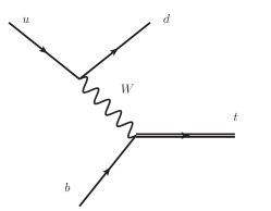
Figure 4: The Feynman diagrams for the single top production via the fusion of a $W$ boson and a bottom quark.

We can take another viewpoint on the t-channel single top production and consider it to be a fusion process, as shown in Fig. 4. An initial state up quark emits a $W$ boson, which then combines with a bottom quark to produce a single top quark. The production of the $W$ boson is similar to a DIS process and there is no specific constraint on the virtuality of the $W$ boson. But when it coannihilates with a bottom quark, the mass of final state top quark impose constraints on the ‘initial’ $W$ boson. As a result, the typical scales of the interactions involving the light quarks and top quarks are $Q$ and $m_{t}$, respectively, which are just about the natural hard scales.

For the jet and soft scales, the situations are not so clear. After inspection of Eqs. (64)-(65) and (72)-(73), one finds that the natural jet and soft scales should be $\sqrt{p^{2}}$ and $2kE_{1}(-\hat{t}+m_{t}^{2})/(-\hat{u})/m_{t}$, respectively. But these two scales are not directly connect to the integration variables in Eq. (III). Moreover, they can become so small that the strong coupling constants in the jet and soft functions would diverge. Therefore, in practice, we choose the natural jet and soft scales numerically.

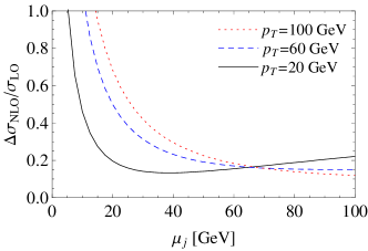
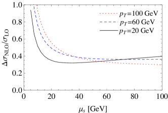
Figure 5: The contributions from jet and soft functions to the NLO cross section.

In Fig. 5, we show the contributions to the NLO cross section from jet and soft functions separately without including the RG evolution effects. We have fixed the top quark transverse momentum to be $p_{T}=20,60,100$ GeV and change the jet (soft) scale from 5 GeV to 100 GeV. It is required that the perturbative expansions of the jet and soft functions converge fast. Thus, we choose the jet and soft scales as 80 GeV and 50 GeV, respectively. When giving the final RG improved cross sections, we will investigate the scale uncertainties due to these choices. From Fig. 5, we can also see that the jet and soft functions give positive contributions to the NLO cross sections, and can be as large as about $20\%$ and $40\%$. To see the corrections from hard functions, in Fig. 6, we show the contributions to the NLO cross section from hard functions.

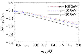
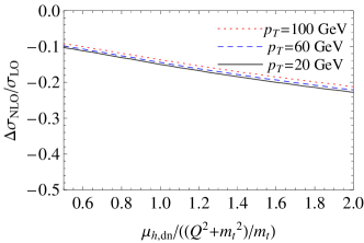
Figure 6: The contributions from hard functions to the NLO cross section.

We find that the hard functions provide negative contributions to the NLO cross sections and the corrections are about $-15\%$ for $\mu_{h,up}=Q$ and $\mu_{h,dn}=(Q^{2}+m_{t}^{2})/m_{t}$.

Before presenting the numerical results for the RG improved cross section, it is important to examine to what extent the singular terms approximate the fixed-order calculation. In Fig. 7, we present the singular terms contribution and fixed-order cross sections.

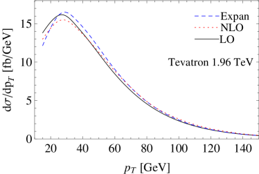
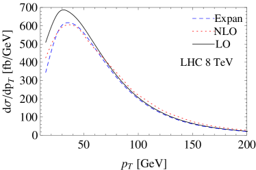
Figure 7: The singular terms contribution and fixed-order cross sections for t-channel single top production at the Tevatron (left) and the LHC (right). The dashed line represents the contributions from the singular terms up to $\mathcal{O}(\alpha_{s}$) which is given in Eq. (87).

We see that the NLO cross section is well approximated by the singular terms when the top quark transverse momentum $p_{T}$ is larger than 50 (70) GeV at the Tevatron (LHC). Therefore, the singular terms should be resummed for the large $p_{T}$ region. For the small $p_{T}$ region, the singular terms do not dominate the NLO corrections, so there is no need to perform resummation in this region. In the following discussion, we will only present the resummation results for $p_{T}>$ 50 (70) GeV at the Tevatron (LHC). Meanwhile we find that the NLO QCD correction is small for t-channel single top production. This is because the large positive soft and jet functions cancel with the large negative hard functions, as discussed in the last paragraph. If these large effects are resummed to higher orders, we can see whether there is still a cancellation between them.

We have chosen all the natural scales involved in this process. Now we give the numerical results of the resummed cross section. When discussing each scale dependence, we fix the other scales at the natural scales discussed above. In Fig. 8, we show the RG improved cross sections as a function of the top quark $p_{T}$. We can see that the distribution is increased by about $9\sim 13\%$ and $4\sim 9\%$ for $p_{T}>$ 50 and 70 GeV at the Tevatron and LHC, respectively, compared to the NLO results.

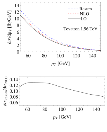
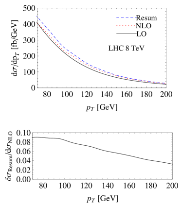
Figure 8: The RG improved (dashed) and fixed-order cross sections for t-channel single top production at the Tevatron (left) and the LHC (right). We have defined $\delta\sigma_{\rm Resum}=d\sigma_{\rm Resum}-d\sigma_{\rm NLO}$.

In Fig. 9, we give the uncertainties of the resummation results due to the change of intermediate scales $\mu_{h,up}$, $\mu_{h,dn}$, $\mu_{j}$, $\mu_{s}$ independently by a factor of two. The uncertainties arising from $\mu_{h,up}$, $\mu_{h,dn}$ and $\mu_{j}$ are less than $\pm 1\%$, and for $\mu_{s}$ are about $\pm 2\%$.

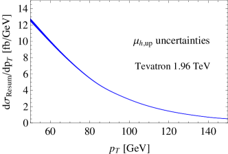
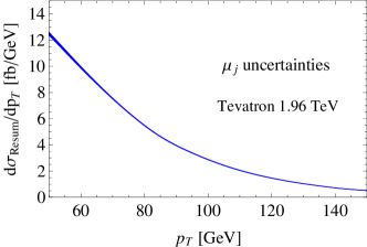
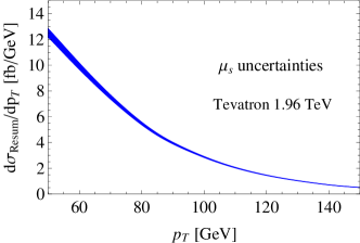
Figure 9: The scale uncertainties of the resummation results due to the variations of $\mu_{h,up}$, $\mu_{h,dn}$, $\mu_{j}$, $\mu_{s}$, respectively.

In Fig. 10, we show the scale uncertainties of the resummation results due to the variations of $\mu_{F,dn}$ and $\mu_{F,up}$ by a factor of two, and do not see scale uncertainties are decreased, compared to the NLO results. In principle, the scale uncertainties should vanish, as illustrated analytically in the last section. However, the analysis there is based on the assumption that the PDF is evaluated near the endpoint. But in practice, this is not always true because the center-of-mass energy of the Tevatron or LHC is much larger than the invariant mass of the final states. And the dynamical enhancement mechanism Becher et al. (2008) is not appropriate for a t-channel process. On the other hand, when approaching the threshold region, i.e., with the increasing of the top quark $p_{T}$, the scale uncertainties of the resummed cross sections are significantly reduced, as shown in Fig. 10.

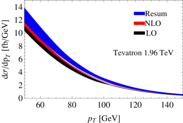
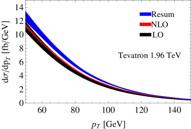
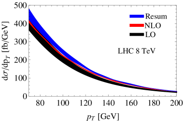
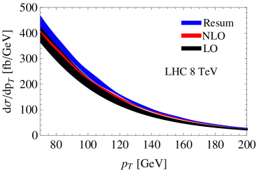
Figure 10: The scale uncertainties due to the variations of $\mu_{F,dn}$ (left) and $\mu_{F,up}$ (right), respectively. The bands in each plots from top to bottom denote the resummation, NLO and LO results, respectively.

VII Conclusion

We have studied the factorization and resummation of t-channel top quark transverse momentum distribution at large $p_{T}$ in the SM at both the Tevatron and the LHC with SCET. This is the first spacelike process studied in SCET involving one massless and one massive colored particles in the final states. The cross section in the threshold region can be factorized into a convolution of hard, jet and soft functions. In particular, we first calculate the NLO soft functions for this process, and give a RG improved cross section by evolving the different functions to a common scale. Our results show that the resummation effects increase the NLO results by about $9\%\sim 13\%$ and $4\%\sim 9\%$ when the transverse momentum of the top quark is larger than $50$ and 70 GeV at the Tevatron and the 8 TeV LHC, respectively. Our prediction on the transverse momentum distribution of the top quark in the large $p_{T}$ region is important in the search for new physics, e.g., a heavy $W^{\prime}$ which can mediate the single top production through the s-channel. Also, we discuss the scale independence of the cross section analytically and show how to choose the proper scales at which the perturbative expansion can converge fast.

Appendix A Calculation of the soft functions

In this appendix, we present the details of the calculation of the two $\mathcal{O}(\alpha_{s})$ soft functions $S^{(1)}_{bt}(k,\mu)$ and $S^{(1)}_{tt}(k,\mu)$. We choose to do the calculation in the rest frame of the top quark, in which the four-velocity of the top quark is $v^{\mu}=(1,0,0,0)$. This choice of frame makes the denominators simple but leaves the complexity in the delta functions. Actually, we also perform the calculation in the frame where the delta functions are simple but the singularities in the denominators are hard to isolate Kelley and Schwartz (2011). And finally we find the same results, which can be considered as a strong cross check for our calculations.

In the rest frame of the top quark, we also choose $n_{b}^{\mu}=(1,0,0,1)$. Then,

$$q^{\mu}=q^{+}\frac{\bar{n}_{b}^{\mu}}{n_{b\bar{b}}}+q^{-}\frac{n_{b}^{\mu}}{n_{b\bar{b}}}+q_{\perp}^{\mu},\quad n_{1}^{\mu}=n_{1}^{+}\frac{\bar{n}_{b}^{\mu}}{n_{b\bar{b}}}+n_{1}^{-}\frac{n_{b}^{\mu}}{n_{b\bar{b}}}+n_{1\perp}^{\mu},$$ (98)

and

$$q\cdot n_{1}=\frac{q^{+}n_{1}^{-}+q^{-}n_{1}^{+}}{n_{b\bar{b}}}-|q_{\perp}||n_{1\perp}|\cos\theta,\quad q\cdot v=q\cdot\frac{(n_{b}+n_{\bar{b}})}{2}=\frac{(q^{+}+q^{-})}{2}.$$ (99)

After putting these expressions into the formula (66), we get

$$S^{(1)}_{bt}(k,\mu) = \frac{g_{s}^{2}C_{F}\mu^{2\epsilon}}{(2\pi)^{d-1}}\int_{0}^{\infty}\mathrm{d}q^{+}\int_{0}^{\infty}\mathrm{d}q^{-}\int\mathrm{d}\Omega_{d-2}\left(\frac{2q^{+}q^{-}}{n_{b\bar{b}}}\right)^{-\epsilon}$$ (100)

$$\delta(k-\frac{q^{+}n_{1}^{-}+q^{-}n_{1}^{+}}{n_{b\bar{b}}}+|q_{\perp}||n_{1\perp}|\cos\theta)\frac{n_{b}\cdot v}{q^{+}(q^{+}+q^{-})}.$$

Now redefine the integration variables $q^{+}$ and $q^{-}$ and let $a=\frac{n_{1}^{+}}{n_{1}^{-}}$, then

$$S^{(1)}_{bt}(k,\mu) = \frac{g_{s}^{2}C_{F}\mu^{2\epsilon}}{(2\pi)^{d-1}}\int_{0}^{\infty}\mathrm{d}q^{+}\int_{0}^{\infty}\mathrm{d}q^{-}\int\mathrm{d}\Omega_{d-2}\left(\frac{2n_{b\bar{b}}}{n_{1}^{+}n_{1}^{-}}\right)^{-\epsilon}$$ (101)

$$\delta(k-q^{+}-q^{-}+2\sqrt{q^{+}q^{-}}\cos\theta)\frac{n_{b}\cdot v}{q^{+}(aq^{+}+q^{-})}.$$

Introducing two variables $x$ and $y$ such that $q^{+}=kyx$ and $q^{-}=ky(1-x)=ky\bar{x}$,

$$S^{(1)}_{bt}(k,\mu)=\frac{g_{s}^{2}C_{F}\mu^{2\epsilon}}{(2\pi)^{d-1}}\left(\frac{2n_{b\bar{b}}}{n_{1}^{+}n_{1}^{-}}\right)^{-\epsilon}k^{-1-2\epsilon}\int\mathrm{d}\Omega_{d-2}\int_{0}^{1}\mathrm{d}xx^{-1-\epsilon}\frac{(1-2\sqrt{x\bar{x}}\cos\theta)^{2\epsilon}\bar{x}^{-\epsilon}}{ax+\bar{x}}.$$ (102)

The singularity in the integrand can be isolated by

$$x^{-1-\epsilon}=-\frac{1}{\epsilon}\delta(x)+\left(\frac{1}{x}\right)_{+}-\epsilon\left(\frac{{\rm ln}x}{x}\right)_{+}+\mathcal{O}(\epsilon^{2}).$$ (103)

After completing the above three parts of the integration separately and expanding

$$\frac{1}{k^{+}}\left(\frac{\tilde{\mu}}{k^{+}}\right)^{2\epsilon}=-\frac{1}{2\epsilon}\delta(k^{+})+\left[\frac{1}{k^{+}}\right]_{\star}^{[k^{+},\tilde{\mu}]}-2\epsilon\left[\frac{1}{k^{+}}{\rm ln}\frac{k^{+}}{\tilde{\mu}}\right]_{\star}^{[k^{+},\tilde{\mu}]}+\mathcal{O}(\epsilon^{2}),$$ (104)

we get the divergent and finite parts

$$S^{(1)}_{bt,div}(k,\mu) = \frac{2C_{F}\alpha_{s}(4\pi\mu^{2}e^{-\gamma_{E}})^{\epsilon}}{4\pi}\biggl{\{}\frac{\delta(k)}{\epsilon^{2}}-\frac{2}{\epsilon}\biggl{[}\frac{1}{k}\biggr{]}_{\star}^{[k,\tilde{\mu}]}\biggr{\}},$$ (105)

$$S^{(1)}_{bt,fin}(k,\mu) = \frac{2C_{F}\alpha_{s}}{4\pi}\biggl{\{}4\biggl{[}\frac{\ln\frac{k}{\tilde{\mu}}}{k}\biggr{]}_{\star}^{[k,\tilde{\mu}]}+\delta(k)c_{bt}^{S}\biggr{\}},$$ (106)

with $c_{bt}^{S}=-{\rm ln}^{2}(1+\frac{1}{a})-2{\rm Li}_{2}(\frac{1}{1+a})+\frac{\pi^{2}}{12}$.

In the same method, we can get

$$S^{(1)}_{tt,div}(k,\mu) = \frac{2C_{F}\alpha_{s}(4\pi\mu^{2}e^{-\gamma_{E}})^{\epsilon}}{4\pi}\biggl{\{}\frac{\delta(k)}{\epsilon}\biggr{\}},$$ (107)

$$S^{(1)}_{tt,fin}(k,\mu) = \frac{2C_{F}\alpha_{s}}{4\pi}\biggl{\{}-\biggl{[}\frac{2}{k}\biggr{]}_{\star}^{[k,\tilde{\mu}]}+\delta(k)c_{tt}^{S}\biggr{\}},$$ (108)

with $c_{tt}^{S}=2{\rm ln}(1+\frac{1}{a})$.

When performing the Laplace transformation from $S(k,\mu)$ to $\widetilde{s}(L,\mu)$, we use the following replacements:

$$\biggl{[}\frac{\ln\frac{k}{\mu}}{k}\biggr{]}_{\star}^{[k,\mu]} \to \frac{L^{2}}{2}+\frac{\pi^{2}}{12},$$ (109)

$$\biggl{[}\frac{1}{k}\biggr{]}_{\star}^{[k,\mu]} \to L.$$ (110)

Appendix B anomalous dimensions

The various anomalous dimensions needed in our calculations can be found, e.g., in Becher et al. (2007, 2008); Becher and Schwartz (2010). We list them below for the convenience of the reader. The QCD $\beta$ function is

$$\beta(\alpha_{s})=-2\alpha_{s}\left[\beta_{0}\frac{\alpha_{s}}{4\pi}+\beta_{1}\left(\frac{\alpha_{s}}{4\pi}\right)^{2}+\cdots\right],$$ (111)

with expansion coefficients

$$\beta_{0} = \frac{11}{3}C_{A}-\frac{4}{3}T_{F}n_{f},$$

$$\beta_{1} = \frac{34}{3}C^{2}_{A}-\frac{20}{3}C_{A}T_{F}n_{f}-4C_{F}T_{F}n_{f},$$

$$\beta_{2} = \frac{2857}{54}C^{3}_{A}+\left(2C^{2}_{F}-\frac{205}{9}C_{F}C_{A}-\frac{1415}{27}C^{2}_{A}\right)T_{F}n_{f}+\left(\frac{44}{9}C_{F}+\frac{158}{27}C_{A}\right)T^{2}_{F}n^{2}_{f},$$ (112)

where $C_{A}=3$, $C_{F}=4/3$, $T_{F}=1/2$ for QCD, and $n_{f}$ is the number of active quark flavors.

The cusp anomalous dimension is

$$\Gamma_{\rm cusp}(\alpha_{s})=\Gamma_{0}\frac{\alpha_{s}}{4\pi}+\Gamma_{1}\left(\frac{\alpha_{s}}{4\pi}\right)^{2}+\cdots,$$ (113)

with

$$\Gamma_{0} = 4C_{F},$$

$$\Gamma_{1} = 4C_{F}\left[\left(\frac{67}{9}-\frac{\pi^{2}}{3}\right)C_{A}-\frac{20}{9}T_{F}n_{f}\right],$$

$$\Gamma_{2} = 4C_{F}\left[C^{2}_{A}\left(\frac{245}{6}-\frac{134}{27}\pi^{2}+\frac{11}{45}\pi^{4}+\frac{22}{3}\zeta_{3}\right)+C_{A}T_{F}n_{f}\left(-\frac{418}{27}+\frac{40}{27}\pi^{2}-\frac{56}{3}\zeta_{3}\right)\right.$$ (114)

$$\left.+C_{F}T_{F}n_{f}\left(-\frac{55}{3}+16\zeta_{3}\right)-\frac{16}{27}T^{2}_{F}n^{2}_{f}\right].$$

The other anomalous dimensions are expanded as Eq. (113), and their expansion coefficients are

$$\gamma^{0}_{q} = -3C_{F},$$

$$\gamma^{1}_{q} = C^{2}_{F}\left(-\frac{3}{2}+2\pi^{2}-24\zeta_{3}\right)+C_{F}C_{A}\left(-\frac{961}{54}-\frac{11}{6}\pi^{2}+26\zeta_{3}\right)+C_{F}T_{F}n_{f}\left(\frac{130}{27}+\frac{2}{3}\pi^{2}\right),$$

$$\gamma^{0}_{Q} = -2C_{F},$$

$$\gamma^{1}_{Q} = C_{F}C_{A}\left(\frac{2}{3}\pi^{2}-\frac{98}{9}-4\zeta_{3}\right)+\frac{40}{9}C_{F}T_{F}n_{f},$$

$$\gamma^{0}_{\phi} = 3C_{F},$$

$$\gamma^{1}_{\phi} = C^{2}_{F}\left(\frac{3}{2}-2\pi^{2}+24\zeta_{3}\right)+C_{F}C_{A}\left(\frac{17}{6}+\frac{22}{9}\pi^{2}-12\zeta_{3}\right)-C_{F}T_{F}n_{f}\left(\frac{2}{3}+\frac{8}{9}\pi^{2}\right),$$

$$\gamma^{0}_{j} = -3C_{F},$$

$$\gamma^{1}_{j} = C^{2}_{F}\left(-\frac{3}{2}+2\pi^{2}-24\zeta_{3}\right)+C_{F}C_{A}\left(-\frac{1769}{54}-\frac{11}{9}\pi^{2}+40\zeta_{3}\right)$$ (115)

$$+C_{F}T_{F}n_{f}\left(\frac{242}{27}+\frac{4}{9}\pi^{2}\right).$$

$\gamma^{V}_{up}$, $\gamma^{V}_{dn}$ and $\gamma^{S}$ can be obtained from the anomalous dimensions above through the following equations:

$$\gamma^{V}_{up} = 2\gamma_{q},$$

$$\gamma^{V}_{dn} = \gamma_{q}+\gamma_{Q},$$

$$\gamma^{S} = -\gamma_{\phi}-\gamma^{V}_{dn}.$$ (116)

References

- Bernreuther (2008) W. Bernreuther, J. Phys. G35, 083001 (2008), eprint 0805.1333.
- Abazov et al. (2009) V. M. Abazov et al. (D0), Phys. Rev. Lett. 103, 092001 (2009), eprint 0903.0850.
- Aaltonen et al. (2009) T. Aaltonen et al. (CDF), Phys. Rev. Lett. 103, 092002 (2009), eprint 0903.0885.
- Aad et al. (2012) G. Aad et al. (ATLAS Collaboration), Physics Letters B 717, 330 (2012), eprint 1205.3130.
- Chatrchyan et al. (2012) S. Chatrchyan et al. (CMS Collaboration) (2012), eprint 1209.4533.
- Bordes and van Eijk (1995) G. Bordes and B. van Eijk, Nucl. Phys. B435, 23 (1995).
- Stelzer and Willenbrock (1995) T. Stelzer and S. Willenbrock, Phys. Lett. B357, 125 (1995), eprint hep-ph/9505433.
- Harris et al. (2002) B. W. Harris, E. Laenen, L. Phaf, Z. Sullivan, and S. Weinzierl, Phys. Rev. D66, 054024 (2002), eprint hep-ph/0207055.
- Sullivan (2004) Z. Sullivan, Phys. Rev. D70, 114012 (2004), eprint hep-ph/0408049.
- Campbell et al. (2004) J. M. Campbell, R. K. Ellis, and F. Tramontano, Phys. Rev. D70, 094012 (2004), eprint hep-ph/0408158.
- Cao and Yuan (2005) Q.-H. Cao and C. P. Yuan, Phys. Rev. D71, 054022 (2005), eprint hep-ph/0408180.
- Cao et al. (2005) Q.-H. Cao, R. Schwienhorst, J. A. Benitez, R. Brock, and C. P. Yuan, Phys. Rev. D72, 094027 (2005), eprint hep-ph/0504230.
- Campbell et al. (2009a) J. M. Campbell, R. Frederix, F. Maltoni, and F. Tramontano, JHEP 10, 042 (2009a), eprint 0907.3933.
- Campbell et al. (2009b) J. M. Campbell, R. Frederix, F. Maltoni, and F. Tramontano, Phys. Rev. Lett. 102, 182003 (2009b), eprint 0903.0005.
- Frixione et al. (2006) S. Frixione, E. Laenen, P. Motylinski, and B. R. Webber, JHEP 03, 092 (2006), eprint hep-ph/0512250.
- Frixione et al. (2008) S. Frixione, E. Laenen, P. Motylinski, B. R. Webber, and C. D. White, JHEP 07, 029 (2008), eprint 0805.3067.
- Alioli et al. (2009) S. Alioli, P. Nason, C. Oleari, and E. Re, JHEP 09, 111 (2009), eprint 0907.4076.
- Kidonakis (2006) N. Kidonakis, Phys. Rev. D74, 114012 (2006), eprint hep-ph/0609287.
- Kidonakis (2007) N. Kidonakis, Phys. Rev. D75, 071501 (2007), eprint hep-ph/0701080.
- Kidonakis (2011) N. Kidonakis, Phys.Rev. D83, 091503 (2011), eprint 1103.2792.
- Bauer et al. (2000) C. W. Bauer, S. Fleming, and M. E. Luke, Phys. Rev. D63, 014006 (2000), eprint hep-ph/0005275.
- Bauer et al. (2001) C. W. Bauer, S. Fleming, D. Pirjol, and I. W. Stewart, Phys. Rev. D63, 114020 (2001), eprint hep-ph/0011336.
- Bauer and Stewart (2001) C. W. Bauer and I. W. Stewart, Phys. Lett. B516, 134 (2001), eprint hep-ph/0107001.
- Bauer et al. (2002) C. W. Bauer, D. Pirjol, and I. W. Stewart, Phys. Rev. D65, 054022 (2002), eprint hep-ph/0109045.
- Becher and Neubert (2006a) T. Becher and M. Neubert, Phys. Rev. Lett. 97, 082001 (2006a), eprint hep-ph/0605050.
- Idilbi and Ji (2005) A. Idilbi and X.-d. Ji, Phys. Rev. D72, 054016 (2005), eprint hep-ph/0501006.
- Idilbi et al. (2005) A. Idilbi, X.-d. Ji, and F. Yuan, Phys. Lett. B625, 253 (2005), eprint hep-ph/0507196.
- Becher et al. (2008) T. Becher, M. Neubert, and G. Xu, JHEP 07, 030 (2008), eprint 0710.0680.
- Stewart et al. (2010) I. W. Stewart, F. J. Tackmann, and W. J. Waalewijn, Phys.Rev. D81, 094035 (2010), eprint 0910.0467.
- Gao et al. (2005) Y. Gao, C. S. Li, and J. J. Liu, Phys. Rev. D72, 114020 (2005), eprint hep-ph/0501229.
- Ahrens et al. (2009a) V. Ahrens, T. Becher, M. Neubert, and L. L. Yang, Phys. Rev. D79, 033013 (2009a), eprint 0808.3008.
- Ahrens et al. (2009b) V. Ahrens, T. Becher, M. Neubert, and L. L. Yang, Eur. Phys. J. C62, 333 (2009b), eprint 0809.4283.
- Zhu et al. (2009) H. X. Zhu, C. S. Li, J. J. Zhang, H. Zhang, and Z. Li, Phys. Rev. D79, 113005 (2009), eprint 0903.5047.
- Mantry and Petriello (2010) S. Mantry and F. Petriello, Phys.Rev. D81, 093007 (2010), eprint 0911.4135.
- Lee and Sterman (2007) C. Lee and G. Sterman, Phys. Rev. D75, 014022 (2007), eprint hep-ph/0611061.
- Fleming et al. (2008a) S. Fleming, A. H. Hoang, S. Mantry, and I. W. Stewart, Phys. Rev. D77, 074010 (2008a), eprint hep-ph/0703207.
- Fleming et al. (2008b) S. Fleming, A. H. Hoang, S. Mantry, and I. W. Stewart, Phys. Rev. D77, 114003 (2008b), eprint 0711.2079.
- Bauer et al. (2008) C. W. Bauer, S. P. Fleming, C. Lee, and G. Sterman, Phys. Rev. D78, 034027 (2008), eprint 0801.4569.
- Schwartz (2008) M. D. Schwartz, Phys. Rev. D77, 014026 (2008), eprint 0709.2709.
- Idilbi et al. (2009) A. Idilbi, C. Kim, and T. Mehen, Phys. Rev. D79, 114016 (2009), eprint 0903.3668.
- Yang et al. (2006) L. L. Yang, C. S. Li, Y. Gao, and J. J. Liu, Phys. Rev. D73, 074017 (2006), eprint hep-ph/0601180.
- Zhu et al. (2011) H. X. Zhu, C. S. Li, J. Wang, and J. J. Zhang, JHEP 1102, 099 (2011), eprint 1006.0681.
- Manohar (2003) A. V. Manohar, Phys. Rev. D68, 114019 (2003), eprint hep-ph/0309176.
- Chay and Kim (2007) J. Chay and C. Kim, Phys. Rev. D75, 016003 (2007), eprint hep-ph/0511066.
- Chen et al. (2007) P.-y. Chen, A. Idilbi, and X.-d. Ji, Nucl. Phys. B763, 183 (2007), eprint hep-ph/0607003.
- Becher and Schwartz (2010) T. Becher and M. D. Schwartz, JHEP 02, 040 (2010), eprint 0911.0681.
- Becher et al. (2012) T. Becher, C. Lorentzen, and M. D. Schwartz, Phys.Rev.Lett. 108, 012001 (2012), eprint 1106.4310.
- Ahrens et al. (2010a) V. Ahrens, A. Ferroglia, M. Neubert, B. D. Pecjak, and L. L. Yang, Phys.Lett. B687, 331 (2010a), eprint 0912.3375.
- Ahrens et al. (2010b) V. Ahrens, A. Ferroglia, M. Neubert, B. D. Pecjak, and L. L. Yang, JHEP 1009, 097 (2010b), eprint 1003.5827.
- Beneke et al. (2012) M. Beneke, P. Falgari, S. Klein, and C. Schwinn, Nucl.Phys. B855, 695 (2012), eprint 1109.1536.
- Chay et al. (2005) J. Chay, C. Kim, Y. G. Kim, and J.-P. Lee, Phys. Rev. D71, 056001 (2005), eprint hep-ph/0412110.
- Korchemsky and Radyushkin (1992) G. Korchemsky and A. Radyushkin, Phys.Lett. B279, 359 (1992), eprint hep-ph/9203222.
- Laenen et al. (1998) E. Laenen, G. Oderda, and G. Sterman, Phys. Lett. B438, 173 (1998), eprint hep-ph/9806467.
- Bauer et al. (2009) C. W. Bauer, A. Hornig, and F. J. Tackmann, Phys. Rev. D79, 114013 (2009), eprint 0808.2191.
- Bauer et al. (2010) C. W. Bauer, N. D. Dunn, and A. Hornig, Phys.Rev. D82, 054012 (2010), eprint 1002.1307.
- Isgur and Wise (1989) N. Isgur and M. B. Wise, Phys. Lett. B232, 113 (1989).
- Ahrens et al. (2012) V. Ahrens, M. Neubert, and L. Vernazza, JHEP 1209, 138 (2012), eprint 1208.4847.
- Becher and Neubert (2009) T. Becher and M. Neubert, Phys. Rev. D79, 125004 (2009), eprint 0904.1021.
- Korchemskaya and Korchemsky (1992) I. Korchemskaya and G. Korchemsky, Physics Letters B 287, 169 (1992).
- Becher et al. (2007) T. Becher, M. Neubert, and B. D. Pecjak, JHEP 01, 076 (2007), eprint hep-ph/0607228.
- Becher and Neubert (2006b) T. Becher and M. Neubert, Phys. Lett. B637, 251 (2006b), eprint hep-ph/0603140.
- (62) Tevatron Electroweak Working Group, CDF and D0 Collaborations (2011), eprint 1107.5255.
- Kelley and Schwartz (2011) R. Kelley and M. D. Schwartz, Phys.Rev. D83, 033001 (2011), eprint 1008.4355.