Conformal Symmetry for Black Holes in Four Dimensions and Irrelevant Deformations

Abstract

It has been argued several times in the past that the structure of the entropy formula for general non-extremal asymptotically flat black holes in four dimensions can be understood in terms of an underlying conformal symmetry. A recent implementation of this idea, carried out by Cvetič and Larsen, involves the replacement of a conformal factor in the original geometry by an alternative conformal factor in such a way that the near-horizon behavior and thermodynamic properties of the black hole remain unchanged, while only the asymptotics or “environment” of the geometry are modified. The solution thus obtained, dubbed “subtracted geometry”, uplifts to an asymptotically AdS${}_{3}\times S^{2}$ black hole in five dimensions, and an AdS/CFT interpretation is then possible. Building on this intuition we show that, at least in the static case, the replacement of the conformal factor can be implemented dynamically by means of an interpolating flow which we construct explicitly. Furthermore, we show that this flow can be understood as the effect of irrelevant perturbations from the point of view of the dual two-dimensional CFT, and we identify the quantum numbers of the operators responsible for the flow. This allows us to address quantitatively the validity of CFT computations for these asymptotically flat black holes and provides a framework to systematically compute corrections to the CFT results.

1 Introduction

Black holes and especially their entropy have always been a source of mystery in physics and, despite decades of effort and remarkable results on this topic, a full understanding of their properties is still lacking. The first microscopic understanding of black hole entropy was achieved for supersymmetric three-charge black holes, where the entropy formula was reproduced using an effective CFT description of the low-energy degrees of freedom Strominger:1996sh . Later developments have expanded upon this description for other extremal and near-extremal black holes David:2002wn ; Kraus:2006wn ; Sen:2007qy . The Kerr/CFT program Guica:2008mu ; Hartman:2008pb ; Compere:2012jk has further provided indications for a CFT description of the low-energy physics for (near-)extremal rotating black holes.

Even when one identifies some sort of conformal symmetry in black hole related backgrounds, this does not need to have immediate physical implications, nor does it have to imply the existence of a CFT whose physics is relevant for the black hole. The connection between the CFT and the black hole can be purely numerological, purely kinematical, approximately dynamical, or exactly dynamical. An example of the latter is the BTZ black hole, whose physics is completely captured by that of a $2d$ CFT. When there is an approximate dynamical equivalence the physical quantities of interest may or may not, depending on the question, be approximately reproduced using CFT computations. In this paper we will mostly be interested in this case.

Unfortunately, a systematic approach to find the approximate dynamical CFT description for the low-energy physics of black holes is still lacking. In general, the low energy near-horizon modes of general black holes (as opposed to (near-)extremal ones) do not seem to decouple from the asymptotics of the geometry, thus effectively preventing one from being able to take a decoupling limit and find an effective CFT description of these modes. Even so, there has been much interest in the fact that the massless wave equation in a (general) black hole background admits a $SL(2,\mathds{R})$ symmetry when certain terms are removed. The offending terms are indeed small and can be neglected in certain limits (near-extremal, near extreme rotating, low energy Cvetic:1997uw ; Maldacena:1996ix ; Guica:2008mu ; Cvetic:2009jn ; Castro:2010fd ). However reminiscent of conformal symmetry this approximate $SL(2,\mathds{R})$ symmetry may be, the terms “breaking” this symmetry are not small for general black holes and thus can not justifiably be ignored. The program of “hidden conformal symmetry” asserts that the conformal symmetry is there after all, but it is spontaneously broken Castro:2010fd .

A recent development by Cvetič and Larsen Cvetic:2011hp ; Cvetic:2011dn , inspired by the approximate $SL(2,\mathds{R})$ symmetry of the massless scalar wave equation, provides further evidence for an approximate CFT description of general black holes in four and five dimensions far from extremality. They construct a so-called “subtracted” geometry, where the warp factor of the geometry is modified. Thus, the asymptotics of the black hole are changed from asymptotically flat to asymptotically conical Cvetic:2012tr , but the thermodynamic properties of the black hole are left untouched. This subtracted geometry can then intuitively be thought of as “putting the black hole in a box”. This subtracted geometry, in addition to providing an exact $SL(2,\mathds{R})$ symmetry of the wave equation, can be uplifted one dimension higher to a geometry that is locally a product of AdS₃ and a two-sphere. Thus, a $2d$ CFT description of this black hole subtracted geometry is immediately obvious.

What is less obvious is the relation between the subtracted geometry and the original, asymptotically flat one, and in particular how this relation would be visible in the CFT description. Further developments Cvetic:2012tr have made some progress in this direction by showing that the subtracted geometry can be obtained as a scaling limit of the original geometry. In this paper, we wish to address this problem and provide further evidence of the $2d$ CFT description of general asymptotically flat, non-rotating, four-charge black holes in four dimensions. If the $2d$ CFT description of the subtracted geometry is related to some IR limit of the asymptotic flat original geometry, then it is natural to expect this original geometry to be described by the CFT plus some irrelevant deformation.

We first construct a family of black hole solutions with various asymptotics in the STU model in four dimensions, of which both the subtracted geometry and the original geometry are members. With this explicit family of solutions, it is easy to find the linear perturbations of the subtracted geometry which must be turned on to flow to the original geometry. These perturbations can then be uplifted to perturbations of AdS${}_{3}\times S^{2}$, where the standard AdS/CFT dictionary allows us to interpret and translate them as irrelevant deformations of the dual $2d$ CFT. We also explicitly determine the sources for these dimension $(2,2)$ operators in the CFT: in addition to providing further insight into the CFT description of asymptotically flat black holes, the explicit construction of these irrelevant operators and their sources allows us to quantitatively determine the limit of the validity of the CFT description.

The rest of the paper is organized as follows. In section 2 we review the STU model and construct a four-parameter family of four-charged, non-rotating black holes with different asymptotics but the same thermodynamics, and explicitly identify the original (asymptotically flat) and subtracted geometry as members of this family. Then, in section 3, we perform a linear analysis to determine the perturbations needed to flow from the subtracted to the original geometry. In section 4 we uplift the subtracted geometry and the linear perturbations thereof to $5d$; we then consistently reduce to an effective three-dimensional description to easily identify the irrelevant operators and sources through the standard AdS/CFT dictionary. The determination of the sources gives us a clear criterion for the window in which the effective IR CFT description is valid. Finally, in section 5, we summarize and discuss our findings. Various details of our calculations and useful formulae are collected in the appendix.

2 The STU model

The STU model is a four-dimensional $\mathcal{N}=2$ supergravity theory coupled to three vector multiplets Cremmer:1984hj ; Duff:1995sm ; Behrndt:1996hu . Its Lagrangian is given by

$$\mathcal{L}_{4}={} R{\,\star_{4}\mathds{1}}-\frac{1}{2}H_{ij}{\,\star_{4}dh^{i}}\wedge dh^{j}-\frac{3}{2f^{2}}{\,\star_{4}df}\wedge df-\frac{f^{3}}{2}{\,\star_{4}F^{0}}\wedge F^{0}$$

$$-\frac{1}{2f^{2}}H_{ij}{\,\star_{4}d\chi^{i}}\wedge d\chi^{j}-\frac{f}{2}H_{ij}{\,\star_{4}}\left(F^{i}+\chi^{i}F^{0}\right)\wedge\left(F^{j}+\chi^{j}F^{0}\right)$$ (1)

$$+\frac{1}{2}C_{ijk}\,\chi^{i}F^{j}\wedge F^{k}+\frac{1}{2}C_{ijk}\,\chi^{i}\chi^{j}F^{0}\wedge F^{k}+\frac{1}{6}C_{ijk}\,\chi^{i}\chi^{j}\chi^{k}F^{0}\wedge F^{0}\,,$$

where the fields $f$ and $h^{i}$ ($i=1,2,3$) are scalars, $\chi^{i}$ are pseudoscalars, and $F^{0}$ and $F^{i}$ are $U(1)$ gauge field strengths. The metric $H_{ij}$ on the scalar moduli space is diagonal with entries $H_{ii}=(h^{i})^{-2}$, and the symbol $C_{ijk}$ is pairwise-symmetric in its indices with $C_{123}=1$ and zero otherwise. The $h^{i}$ fields are constrained by the relation $h^{1}h^{2}h^{3}=1$, which must be solved before taking variations of the action. Our conventions for Hodge duality as well as some useful expressions can be found in appendix A.1.

In the following we shall be concerned with solutions where the pseudoscalars $\chi^{i}$ are set to zero. This is not in general a consistent truncation, inasmuch as the pseudoscalar equations of motion then imply the constraints

$$-f\,H_{ij}{\,\star_{4}F^{0}}\wedge F^{j}+\frac{1}{2}C_{ijk}\,F^{j}\wedge F^{k}=0\,.$$ (2)

In order to fulfill these conditions we will consider solutions where $F^{0}$ is purely electric and the $F^{i}$ are purely magnetic. If we restrict to this case, we can write a simpler action from which we can derive the equations of motion, namely

$$S=-\frac{1}{2\kappa^{2}}\int d^{4}x\sqrt{|g|}\biggl{[}R-\frac{e^{-\eta_{0}}}{4}F_{\mu\nu}^{0}F^{0\,\mu\nu}-\frac{1}{2}\sum_{i=1}^{3}\biggl{(}\nabla_{\mu}\eta_{i}\nabla^{\mu}\eta_{i}+\frac{e^{2\eta_{i}-\eta_{0}}}{2}F_{\mu\nu}^{i}F^{i\,\mu\nu}\biggr{)}\biggr{]},$$ (3)

where $\kappa^{2}=8\pi G_{4}$ ($\kappa$ has units of length), and we have introduced the shorthand notation

$$\eta_{0}\equiv\eta_{1}+\eta_{2}+\eta_{3}\,.$$ (4)

The scalar fields $\eta_{i}$ ($i=1,2,3$) are related to the scalars in (1) through

$$h^{i} =e^{\frac{1}{3}\eta_{0}-\eta_{i}}\,,$$ (5)

$$f =e^{-\frac{1}{3}\eta_{0}}\,.$$ (6)

The corresponding equations of motion read

$$0={} \nabla_{\mu}\nabla^{\mu}\eta_{i}+\frac{1}{4}\Biggl{[}e^{-\eta_{0}}F^{0}_{\mu\nu}F^{0\mu\nu}+e^{-\eta_{0}}\sum_{j=1}^{3}\bigl{(}1-2\delta_{ij}\bigr{)}e^{2\eta_{j}}F_{\mu\nu}^{j}F^{j\mu\nu}\Biggr{]},$$ (7)

$$0={} \nabla_{\mu}\Bigl{(}e^{-\eta_{0}}F^{0\,\mu\nu}\Bigr{)},$$ (8)

$$0={} \nabla_{\mu}\Bigl{(}e^{-\eta_{0}+2\eta_{i}}F^{i\,\mu\nu}\Bigr{)},$$ (9)

$$G_{\mu\nu}={} \frac{1}{2}\Biggl{[}\sum_{i=1}^{3}\left(\nabla_{\mu}\eta_{i}\nabla_{\nu}\eta_{i}-\frac{g_{\mu\nu}}{2}\nabla_{\lambda}\eta_{i}\nabla^{\lambda}\eta_{i}\right)$$

$$+e^{-\eta_{0}}\left(F^{0\,\rho}_{\mu}F^{0}_{\nu\rho}-\frac{g_{\mu\nu}}{4}F^{0}_{\lambda\rho}F^{0\,\lambda\rho}\right)+e^{-\eta_{0}}\sum_{i=1}^{3}e^{2\eta_{i}}\left(F^{i\,\rho}_{\mu}F^{i}_{\nu\rho}-\frac{g_{\mu\nu}}{4}F^{i}_{\lambda\rho}F^{i\,\lambda\rho}\right)\Biggr{]}.$$ (10)

2.1 Static ansatz

In the present context we will be interested in static, spherically symmetric black hole backgrounds. As discussed above, in order to fulfill the constraint (2) we furthermore consider an electric ansatz for $F^{0}$ and a magnetic ansatz for the $F^{i}$. Explicitly, our ansatz for the metric and matter fields reads

$$ds_{4}^{2}={} -\frac{G(r)}{\sqrt{\Delta(r)}}dt^{2}+\sqrt{\Delta(r)}\left(\frac{dr^{2}}{X(r)}+d\theta^{2}+\frac{X(r)}{G(r)}\sin^{2}\theta\,d\phi^{2}\right)$$ (11)

$$A^{0}={} A^{0}_{t}(r)\,dt$$ (12)

$$A^{i}={} B_{i}\cos\theta\,d\phi$$ (13)

$$\eta_{i}={} \eta_{i}(r)\,,$$ (14)

where the constants $B^{i}$ ($i=1,2,3$) are the magnetic charges. Einstein’s equations are easily seen to imply $G(r)=\gamma X(r)$, where $\gamma=const$, and also $X^{\prime\prime}(r)=2$. Hence, without loss of generality we set

$$X(r)=G(r)=r^{2}-2mr\,.$$ (15)

Given this ansatz, we first notice that the equation for $F^{0}$ implies

$$F^{0}_{rt}=q_{0}\frac{e^{\eta_{0}}}{\sqrt{\Delta}}\,,$$ (16)

where the constant $q_{0}$ is the electric charge (up to normalization). The scalar equations then reduce to

$$0={} \Bigl{(}r(r-2m)\eta_{i}^{\prime}\Bigr{)}^{\prime}-\frac{e^{\eta_{0}}}{2\sqrt{\Delta}}\left[q_{0}^{2}+\sum_{j=1}^{3}\left(2\delta_{ij}-1\right)B_{j}^{2}\,e^{2\left(\eta_{j}-\eta_{0}\right)}\right].$$ (17)

Finally, one notices that the independent information contained in Einstein’s equations amounts to one second order and one first order equation. These can be taken to be

$$0={} \frac{\Delta^{\prime\prime}}{\Delta}-\frac{3}{4}\left(\frac{\Delta^{\prime}}{\Delta}\right)^{2}+\left(\eta_{1}^{\prime}\right)^{2}+\left(\eta_{2}^{\prime}\right)^{2}+\left(\eta_{3}^{\prime}\right)^{2}$$ (18)

$$0={} \left(\frac{\Delta^{\prime}}{2\Delta}\right)^{2}-\frac{2(r-m)}{r(r-2m)}\frac{\Delta^{\prime}}{\Delta}+\frac{4}{r(r-2m)}+\left(\eta_{1}^{\prime}\right)^{2}+\left(\eta_{2}^{\prime}\right)^{2}+\left(\eta_{3}^{\prime}\right)^{2}$$

$$-\frac{e^{\eta_{0}}}{r(r-2m)\sqrt{\Delta}}\left[q_{0}^{2}+\sum_{i=1}^{3}e^{-2\left(\eta_{0}-\eta_{i}\right)}B_{i}^{2}\right].$$ (19)

The first of these equations is a linear combination of the $(t,t)$ and $(\phi,\phi)$ components of Einstein’s equations, while the first order constraint is the $(r,r)$ component.

2.2 Diagonalizing the non-linear system: decoupled modes and a family of static black hole solutions

Quite remarkably, it is possible to diagonalize the full non-linear system of equations. To this end we introduce new fields $\phi_{0}$, $\phi_{i}$ defined as

$$\phi_{0}(r) =\frac{1}{2}\log\left(\frac{\Delta(r)}{m^{4}}\right)-\eta_{1}(r)-\eta_{2}(r)-\eta_{3}(r)$$ (20)

$$\phi_{1}(r) =\frac{1}{2}\log\left(\frac{\Delta(r)}{m^{4}}\right)-\eta_{1}(r)+\eta_{2}(r)+\eta_{3}(r)$$ (21)

$$\phi_{2}(r) =\frac{1}{2}\log\left(\frac{\Delta(r)}{m^{4}}\right)+\eta_{1}(r)-\eta_{2}(r)+\eta_{3}(r)$$ (22)

$$\phi_{3}(r) =\frac{1}{2}\log\left(\frac{\Delta(r)}{m^{4}}\right)+\eta_{1}(r)+\eta_{2}(r)-\eta_{3}(r)\,.$$ (23)

Taking suitable linear combinations of the scalar and Einstein’s equations one finds

$$0={} \Bigl{(}r\left(r-2m\right)\phi_{0}^{\prime}(r)\Bigr{)}^{\prime}+2\left(\frac{q_{0}^{2}}{m^{2}}\,e^{-\phi_{0}(r)}-1\right)$$ (24)

$$0={} \Bigl{(}r\left(r-2m\right)\phi_{i}^{\prime}(r)\Bigr{)}^{\prime}+2\left(\frac{B_{i}^{2}}{m^{2}}e^{-\phi_{i}(r)}-1\right)\,.$$ (25)

Upon solving these decoupled equations one has the solution for the original fields $\Delta(r)$ and $\eta_{i}(r)$, and the solution for $F^{0}$ is then given by (16). Hence, we have effectively diagonalized the full non-linear system.

We have obtained general solutions to the decoupled equations (24)-(25), each of which depends on two arbitrary integration constants. These generic solutions are not regular at the horizon $r=2m\,$, but upon imposing regularity they reduce to

$$\phi_{0}^{\text{reg}}(r) =\log\left[\frac{q_{0}^{2}}{4m^{4}}\frac{\left(a_{0}^{2}\,r+2m\right)^{2}}{1+a_{0}^{2}}\right]$$ (26)

$$\phi_{j}^{\text{reg}}(r) =\log\left[\frac{B_{j}^{2}}{4m^{4}}\frac{\left(a_{j}^{2}\,r+2m\right)^{2}}{1+a_{j}^{2}}\right],$$ (27)

where the four independent constants $a_{0}$, $a_{i}$ parameterize a family of static black hole solutions. Close to the horizon, one finds

$$\phi_{0}^{\text{reg}}(r\to 2m) =\log\Bigl{(}\frac{q_{0}^{2}}{m^{2}}\left(1+a_{0}^{2}\right)\Bigr{)}+\mathcal{O}\bigl{(}r-2m\bigr{)}\,,$$ (28)

$$\phi_{j}^{\text{reg}}(r\to 2m) =\log\Bigl{(}\frac{B_{j}^{2}}{m^{2}}\left(1+a_{j}^{2}\right)\Bigr{)}+\mathcal{O}\bigl{(}r-2m\bigr{)}\,.$$ (29)

Similarly, in the asymptotic region $r\to\infty$

$$\phi_{0}^{\text{reg}}(r\to\infty) =\left\{\begin{array}[]{rrr}\log\frac{r^{2}}{m^{2}}+\mathcal{O}\left(1\right)\,,&&a_{0}\neq 0\\ \log\frac{q_{0}^{2}}{m^{2}}\,,&&a_{0}=0\end{array}\right.$$ (32)

$$\phi_{j}^{\text{reg}}(r\to\infty) =\left\{\begin{array}[]{rrr}\log\frac{r^{2}}{m^{2}}+\mathcal{O}\left(1\right)\,,&&a_{j}\neq 0\\ \log\frac{B_{j}^{2}}{m^{2}}\,,&&a_{j}=0\end{array}\right.$$ (35)

Going back to the original fields $\eta_{i}$ and $\Delta$, the solution reads

$$\Delta(r)={} \frac{\sqrt{q_{0}^{2}B_{1}^{2}B_{2}^{2}B_{3}^{2}}}{16m^{4}}\prod_{I=0}^{3}\frac{a_{I}^{2}\,r+2m}{\sqrt{1+a_{I}^{2}}}$$ (36)

$$e^{2\eta_{1}(r)}={} \left|\frac{B_{2}B_{3}}{q_{0}B_{1}}\right|\sqrt{\frac{\left(1+a_{0}^{2}\right)\left(1+a_{1}^{2}\right)}{\left(1+a_{2}^{2}\right)\left(1+a_{3}^{2}\right)}}\frac{\left(a_{2}^{2}\,r+2m\right)\left(a_{3}^{2}\,r+2m\right)}{\left(a_{0}^{2}\,r+2m\right)\left(a_{1}^{2}\,r+2m\right)}$$ (37)

$$e^{2\eta_{2}(r)}={} \left|\frac{B_{1}B_{3}}{q_{0}B_{2}}\right|\sqrt{\frac{\left(1+a_{0}^{2}\right)\left(1+a_{2}^{2}\right)}{\left(1+a_{1}^{2}\right)\left(1+a_{3}^{2}\right)}}\frac{\left(a_{1}^{2}\,r+2m\right)\left(a_{3}^{2}\,r+2m\right)}{\left(a_{0}^{2}\,r+2m\right)\left(a_{2}^{2}\,r+2m\right)}$$ (38)

$$e^{2\eta_{3}(r)}={} \left|\frac{B_{1}B_{2}}{q_{0}B_{3}}\right|\sqrt{\frac{\left(1+a_{0}^{2}\right)\left(1+a_{3}^{2}\right)}{\left(1+a_{1}^{2}\right)\left(1+a_{2}^{2}\right)}}\frac{\left(a_{1}^{2}\,r+2m\right)\left(a_{2}^{2}\,r+2m\right)}{\left(a_{0}^{2}\,r+2m\right)\left(a_{3}^{2}\,r+2m\right)}\,.$$ (39)

It is worth emphasizing that, depending on how many of the constants $a_{0}$, $a_{i}\,$ are non-zero, the asymptotic behavior of $\Delta(r)$ in our family of solutions can be of the form $\Delta(r\to\infty)\sim r^{\gamma}$, with $\gamma=0,1,\ldots,4\,$. In particular, when $a_{0}=a_{i}=0$ (i.e. $\gamma=0$) we obtain an asymptotically AdS${}_{2}\times S^{2}$ black hole solution. When $\gamma\neq 0$, the metric displays a “Lifshitz-covariance” of the form $t\to\lambda^{z}t\,$, $r\to\lambda^{2\theta/\gamma}r\,$, $ds^{2}\to\lambda^{\theta}ds^{2}\,$ in the $r\gg 2m$ region, where the dynamical exponent $z$ and the hyperscaling violation exponent $\theta$ are related by $\theta=\left(\frac{\gamma}{\gamma-2}\right)z$. We have checked explicitly that our family of solutions satisfies all the coupled equations of motion. In particular, the first order constraint (19) is satisfied identically, and places no restriction on the values of the constants $a_{0}$, $a_{i}$.

2.3 The “original” and “subtracted” geometries

The family of solutions found in section 2.2 contains as a particular case the solutions dubbed “original” and “subtracted” in Cvetic:2011hp ; Cvetic:2011dn . The original solution is given in terms of functions

$$p_{I}(r)=r+2m\sinh^{2}\delta_{I}\,,$$ (40)

($I=0,1,2,3$) and it reads

$$\Delta(r)={} \prod_{I=0}^{3}p_{I}(r)$$ (41)

$$e^{-\eta_{i}(r)}={} p_{i}(r)\sqrt{\frac{p_{0}(r)}{p_{1}(r)p_{2}(r)p_{3}(r)}}$$ (42)

$$F_{rt}^{0}={} -m\frac{\sinh\left(2\delta_{0}\right)}{p_{0}(r)^{2}}\,.$$ (43)

We then see that the original geometry is asymptotically flat in the $r\to\infty$ (i.e. $r\gg 2m$) region. Comparing with our general solution we can easily read off the electric and magnetic charges and the parameters $a_{I}$ in terms of the $\delta_{I}$:

$$q_{0}^{\text{orig}}=-m\sinh(2\delta_{0})\,,\quad B_{i}^{\text{orig}}=m\sinh\left(2\delta_{i}\right),$$ (44)

$$a_{I}^{\text{orig}}=\frac{1}{\sinh(\delta_{I})}\,.$$ (45)

Similarly, the so-called subtracted geometry is given by

$$\Delta(r)={} (2m)^{3}\Bigl{[}\left(\Pi_{c}^{2}-\Pi_{s}^{2}\right)r+2m\,\Pi_{s}^{2}\Bigr{]}$$ (46)

$$e^{\eta_{i}(r)}={} \frac{1}{\sqrt{\Delta(r)}}\prod_{j\neq i}B_{j}$$ (47)

$$F_{tr}^{0}={} -\frac{16m^{4}}{\Delta^{2}(r)}\Pi_{c}\Pi_{s}B_{1}B_{2}B_{3}\,,$$ (48)

where the $B_{i}$ are the magnetic charges as before, and we can read off the electric charge as $q_{0}=-16m^{4}\left(B_{1}B_{2}B_{3}\right)^{-1}\Pi_{c}\Pi_{s}$. This solution is asymptotically conical for $r\rightarrow\infty$ Cvetic:2012tr . Comparing with our general solution, we learn that the subtracted geometry has

$$a_{0}^{\text{subt}}=\sqrt{\frac{\Pi_{c}^{2}-\Pi_{s}^{2}}{\Pi_{s}^{2}}}\,,\qquad a^{\text{subt}}_{i}=0\,.$$ (49)

As shown in Cvetic:2011hp , the thermodynamics of the original and subtracted solutions matches if the parameters $\Pi_{c}$ and $\Pi_{s}$ are given as follows:

$$\Pi_{c}=\prod_{I=0}^{3}\cosh\delta_{I}\,,\qquad\Pi_{s}=\prod_{I=0}^{3}\sinh\delta_{I}\,.$$ (50)

As we indicated above, depending on how many of the parameters $a_{I}$ are zero the (large-$r$) asymptotic behavior of the conformal factor $\Delta(r)$ changes. While the asymptotically flat original geometry has all $a_{I}\neq 0$ and $\Delta_{\text{orig}}\sim r^{4}$ for large $r$ (i.e. $r\gg 2m$), we have shown that the subtracted solution has $a_{1}=a_{2}=a_{3}=0$ and therefore the conformal factor scales linearly $\Delta_{\text{subt}}\sim r$. Figure 1 illustrates how we can smoothly interpolate between the subtracted and original geometries by dialing the parameters $a_{I}$. In particular notice that when all $\delta_{i}\gg 1$ a region emerges where the two solutions match to a very good approximation. It is in this sense that we refer to our family of solutions as an interpolating flow, with the different curves in figure 1 corresponding to different points in the space of couplings on a putative dual field theory. In fact, in this limit (also known as dilute-gas approximation) one can think of the subtracted solution as coming from a decoupling limit of the original solution, as we will discuss in the next sections.

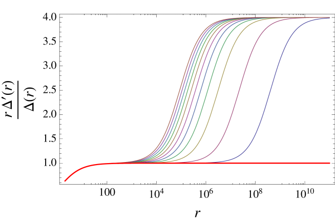
Figure 1: Log plot of $\gamma(r)\equiv\frac{d\log(\Delta)}{d\log r}$ for the general solution (36). The bottom red curve with $\gamma(r\gg 2m)=1$ corresponds to the subtracted geometry ($a_{1}=a_{2}=a_{3}=0$), while the various curves with $\gamma(r\gg 2m)=4$ correspond to the original geometry with different values for $a_{1}=a_{2}=a_{3}\equiv 1/\sinh(\delta)$. The different curves have increasingly larger values of $\delta$ towards the right, so we see that the original and subtracted geometries agree over a broader range in $r$ as the magnetic charges $B\sim\sinh(2\delta)$ increase.

3 Interpreting the flow between the original and subtracted geometries

In the previous section we described a four-parameter family of exact static solutions of the STU model that interpolates between the original and subtracted geometries; depending on the choice of parameters, this family also includes geometries with different asymptotic behavior from that of the original geometry. We can thus view the subtracted geometry loosely as an IR endpoint of an RG flow starting from the original geometry.
It is noteworthy that our solution implements explicitly the scaling limit discussed in Cvetic:2012tr that extracts the subtracted solution from the original one. In the present section we will interpret this scaling limit as a flow between the original and subtracted geometries, while setting the stage for the AdS/CFT discussion to follow in section 4.

Even though (36)-(39) (with $F^{0}$ given by (16)) is an exact solution of the full nonlinear equations, we find it instructive to discuss its linearized version. On the one hand the linearized analysis makes the discussion of regularity at the horizon cleaner, since this is related to a choice of state in the holographic context. Secondly, the sources that one gets by linearizing our family of exact solutions do not necessarily correspond to the sources of irrelevant perturbation theory, as we will discuss in detail below. Lastly, while in generic situations exact solutions to the nonlinear equations are not available, the principles behind the linearized analysis still apply. In particular, we will exhibit the existence of linearized modes of the subtracted geometry that start the flow to the original geometry when their sources are chosen correctly. As we will explicitly show in section 4, upon uplifting the solutions to $5d$, these modes will turn out to be dual to irrelevant operators that deform the conformal field theory dual to the subtracted geometry.

3.1 Linearized analysis

We start our analysis by linearizing the field equations around the subtracted solution. Since the full non-linear equations of motion are diagonalized by the fields $\phi_{I}$ in (20)-(23), we can simply consider

$$\phi_{I}=\phi_{I}^{\text{subt}}+\delta\phi_{I}\,,$$ (51)

where the $\delta\phi_{I}$ will be our linearized perturbations. The linearized equations are then

$$r(r-2m)\delta\phi_{0}^{\prime\prime}+2(r-m)\delta\phi_{0}^{\prime}-2\frac{q_{0}^{2}B_{1}^{2}B_{2}^{2}B_{3}^{2}}{\Delta^{2}}\delta\phi_{0}=0\,,$$ (52)

$$r(r-2m)\delta\phi_{i}^{\prime\prime}+2(r-m)\delta\phi_{i}^{\prime}-2\delta\phi_{i}=0\,.$$ (53)

The equations for the $\delta\phi_{i}$’s are particularly simple, and we focus on those first. Changing to a new radial variable $x=\frac{r}{m}-1\,$, these equations take the form

$$(1-x^{2})\delta\phi_{i}^{\prime\prime}(x)-2x\delta\phi_{i}^{\prime}(x)+2\delta\phi_{i}(x)=0\,,$$ (54)

which is a Legendre equation whose general solution is

$$\delta\phi_{i}(x)=\alpha_{i}\,x+\beta_{i}\left(\frac{x}{2}\log\left(\frac{x+1}{x-1}\right)-1\right).$$ (55)

Of these two solutions, only one is regular at the horizon (which is located at $x=1$), therefore we must set $\beta_{i}=0$, or

$$\delta\phi_{i}=\alpha_{i}\left(\frac{r}{m}-1\right).$$ (56)

Using the same variable $x$, and defining the parameters $b$ and $c$ as

$$b=\frac{\Pi_{c}^{2}-\Pi_{s}^{2}}{2\sqrt{2}\Pi_{c}\Pi_{s}}\,,\qquad c=\frac{\Pi_{c}^{2}+\Pi_{s}^{2}}{2\sqrt{2}\Pi_{c}\Pi_{s}}\,,$$ (57)

the equation for $\delta\phi_{0}$ becomes

$$(1-x^{2})\delta\phi_{0}^{\prime\prime}(x)-2x\delta\phi_{0}^{\prime}(x)+\frac{1}{(bx+c)^{2}}\delta\phi_{0}(x)=0\,.$$ (58)

The solution that is regular at the horizon in this case is given by

$$\delta\phi_{0}=\alpha_{0}\frac{cx+b}{bx+c}=\alpha_{0}\frac{(\Pi_{c}^{2}+\Pi_{s}^{2})r-2m\Pi_{s}^{2}}{(\Pi_{c}^{2}-\Pi_{s}^{2})r+2m\Pi_{s}^{2}}\,.$$ (59)

Notice that the condition of regularity will translate into a functional relation between the normalizable and non-normalizable modes in the standard holographic setting.

3.2 Perturbation theory and determination of the sources

In the previous section we showed that the solutions dubbed “original” and “subtracted” fit in a four-parameter family of solutions parametrized by $a_{I}$. In particular, recall that we have

$$a^{\text{orig}}_{i}=\frac{1}{\sinh\delta_{i}}\,,\qquad a^{\text{subt}}_{i}=0\,,$$ (60)

while the two $a_{0}$’s are both different from zero. In order to go from the subtracted to the original geometry, we need to “turn on” the parameters $a_{i}$ and change the parameter $a_{0}$. We would like to understand this in terms of a flow that is started by linearized fluctuations around the subtracted background. This suggests that the sources $\alpha_{I}$ should be directly related to the parameters $a_{I}$. However, since we are turning on an irrelevant mode, at each order in perturbation theory higher powers of $r$ will be generated, therefore we need to treat the sources as infinitesimal quantities. It is easy to see that linearizing the general solution $\phi_{i}$ around $a_{i}^{2}=0$, at first order in $a_{i}^{2}$ one gets:

$$\phi_{i}=\phi_{i}^{\text{subt}}+a_{i}^{2}\left(\frac{r}{m}-1\right)+\ldots\,,$$ (61)

and we recognize the second term on the right-hand side as being the linearized perturbation of the previous subsection. Notice that the higher order terms do not contain terms linear in $r$, so the sources obtained by linearizing in $a_{i}^{2}$ are equivalent to the sources that one would obtain by extracting the coefficient of order $r$ in a power-series expansion. Therefore we should identify

$$\alpha_{i}=(a^{\text{orig}}_{i})^{2}=\frac{1}{\sinh^{2}\delta_{i}}\,.$$ (62)

Analogously, we have

$$\phi_{0}=\phi_{0}^{\text{subt}}+(a_{0}^{2}-(a^{\text{subt}}_{0})^{2})\frac{\Pi_{s}^{2}}{\Pi_{c}^{2}}\frac{(\Pi_{c}^{2}+\Pi_{s}^{2})r-2m\Pi_{s}^{2}}{(\Pi_{c}^{2}-\Pi_{s}^{2})r+2m\Pi_{s}^{2}}\,,$$ (63)

and as a consequence

$$\alpha_{0}=\left((a^{\text{orig}}_{0})^{2}-(a^{\text{subt}}_{0})^{2}\right)\frac{\Pi_{s}^{2}}{\Pi_{c}^{2}}\,.$$ (64)

Notice however that the sources are in general not infinitesimal. They do become infinitesimal in the limit where the three parameters $\delta_{i}$ become very large. In fact in this limit we obtain particularly simple expressions for the sources:

$$\alpha_{i} \approx 4\,e^{-2\delta_{i}}\,,$$ (65)

$$\alpha_{0} \approx-4\sum_{i}e^{-2\delta_{i}}\,.$$ (66)

Therefore, to leading order we have the relation:

$$\frac{\delta\Delta}{\Delta}=\frac{1}{2}\sum_{I}\delta\phi_{I}=0,$$ (67)

that is, the metric is not changed to leading order in the parameters $e^{-2\delta_{i}}$.

Looking at the behavior of the linearized modes for very large $r$, one is led to the suspicion that the $\delta\phi_{i}$’s correspond to irrelevant perturbations while $\delta\phi_{0}$ seems to be associated to a marginal perturbation. In section 4 we will show that this suspicion is correct (after a suitable change of basis), and we will compute the quantum numbers of the operators in the dual CFT₂ that we need to turn on to start the flow to the asymptotically flat original black hole. It is important to notice that these irrelevant perturbations do change the value of the matter fields in the interior, and in particular they are finite (i.e. non zero) at the horizon. This is in contrast to the extremal case, where irrelevant perturbations die off quickly in the interior and do not change the value of the fields at the horizon.

Notice also that since we are turning on irrelevant deformations, there is no intrinsic (i.e. coordinate invariant) way to extract the sources for the dual operators. Their precise definitions must be supplemented with a perturbation scheme to compute higher order corrections. For example, it is easy to see that our choice for the $\alpha_{i}$’s is compatible with a scheme where the linear term in $r$ does not receive higher order corrections; however if we used a different radial coordinate, for example $r^{\prime}=r+c$ where $c$ is a constant, this would not be true anymore. This ambiguity has an analog in quantum field theory, where the question of whether a source of an operator receives quantum corrections or not depends on the renormalization scheme. This ambiguity is obviously not present to leading order in perturbation theory. We will revisit this issue at the end of section 4.3, where we will describe other possible choices for the sources.

3.3 Range of validity of the linear approximation

In many applications, one does not have the exact solutions, and often it is even impossible to solve the linearized equations exactly. In fact, in many interesting situations only the linearized modes in the asymptotic region are available, and a numerical treatment becomes necessary. It is therefore useful to investigate how one could approach this problem from a numerical perspective; we will then be able to compare the numerical results with the analytic results of the previous sections. The first step is to find a region that can be identified with the asymptotic region of the subtracted geometry (that is $\frac{r}{m}\gg 1$) but where the modes that start the flow to the original geometry are still small, so that they can be treated perturbatively. From the discussion in the previous sections, it is clear that this region should be

$$1<\frac{r}{m}\ll\frac{1}{\alpha}\,.$$ (68)

where $\alpha$ is the smallest of the $\alpha_{i}$’s. Furthermore, we argued that the $\alpha_{i}$’s are related to the parameters $\delta_{i}$, so that when the latter are large, $\alpha_{i}\approx 4\,e^{-2\delta_{i}}$. As anticipated in the previous section, this is when the three charges $B_{1}$, $B_{2}$, and $B_{3}$ are large compared to the fourth, $q_{0}\,$.

Since we expect the difference between the original and subtracted solutions for the $\phi_{i}$’s to be linear in this intermediate region, it is possible to determine the sources for these three modes by means of a linear interpolation, as shown in figure 2. The slope of the linear function turns out to be $4e^{-2\delta_{i}}$, perfectly matching the results of the previous section.

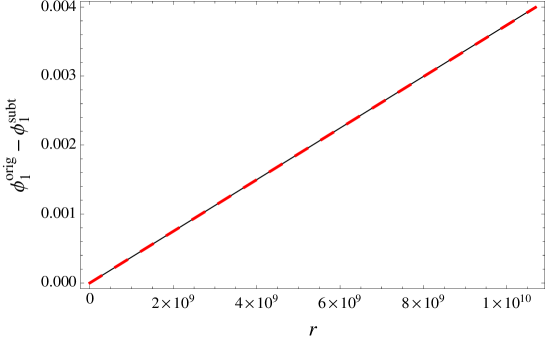
Figure 2: The dashed red line represents the difference between the original and subtracted fields $\phi_{1}\,$. The solid black line is a linear function with slope $4e^{-2\delta_{1}}$. For this plot, we chose $\delta_{0}=\delta_{1}=\delta_{2}=\delta_{3}=15$, $m=1$, and the domain is $r\in[100,10^{-4}e^{2\delta_{1}}]\,$.

We can also plot $\phi_{0}$ and the function $\alpha_{0}\frac{(\Pi_{c}^{2}+\Pi_{s}^{2})r-2m\Pi_{s}^{2}}{(\Pi_{c}^{2}-\Pi_{s}^{2})r+2m\Pi_{s}^{2}}$. We see in figure 3 that the correct source for this mode is $\alpha_{0}=-\alpha_{1}-\alpha_{2}-\alpha_{3}=-4(e^{-2\delta_{1}}+e^{-2\delta_{2}}+e^{-2\delta_{3}})$, confirming once again the analysis of the previous section. Before closing this section it is worth emphasizing that, by turning on different combinations of the sources, we can also flow to the various geometries with Lifshitz-like scaling discussed in section 2.2.

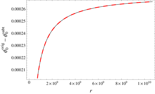
Figure 3: The dashed red line represents the difference between the original and subtracted fields $\phi_{0}\,$. The solid black line is the function $4(e^{-2\delta_{1}}+e^{-2\delta_{2}}+e^{-2\delta_{3}})\frac{(\Pi_{c}^{2}+\Pi_{s}^{2})r-2m\Pi_{s}^{2}}{(\Pi_{c}^{2}-\Pi_{s}^{2})r+2m\Pi_{s}^{2}}$. For this plot, we chose $\delta_{0}=\delta_{1}=\delta_{2}=\delta_{3}=15$, $m=1$, and the domain is $r\in[100,10^{-4}e^{2\delta_{1}}]\,$.

4 Uplifting and AdS/CFT interpretation

In this section we uplift our $4d$ solutions to five dimensions, where an AdS/CFT interpretation of the flow is possible. As shown in Cvetic:2011hp , the subtracted geometry uplifts to a BTZ black hole, which is asymptotically AdS${}_{3}\times S^{2}$. The linearized perturbations of the previous section uplift to linearized perturbations of the BTZ black hole, and we will explicitly show them to be dual to three irrelevant scalar operators with conformal weights $(h,\bar{h})=(2,2)$. This allows us to give a more precise description of the dynamical realization of the conformal symmetry for the charged $4d$ black holes under study, while clarifying at the same time the limitations of this program.

4.1 The $5d$ Lagrangian and equations of motion

As shown in Virmani:2012kw , the STU model (1) can be obtained by dimensional reduction of the following $5d$ Lagrangian:

$$\mathcal{L}_{5}=R_{5}{\,\star_{5}\mathds{1}}-\frac{1}{2}H_{ij}{\,\star_{5}dh^{i}}\wedge dh^{j}-\frac{1}{2}H_{ij}{\,\star_{5}\tilde{F}^{i}}\wedge\tilde{F}^{j}+\frac{1}{6}C_{ijk}\,\tilde{F}^{i}\wedge\tilde{F}^{j}\wedge\tilde{A}^{k},$$ (69)

where $H_{ij}$ and $C_{ijk}$ are defined as in (1). The $4d$ and $5d$ line elements are related by

$$ds_{5}^{2}=f^{-1}ds_{4}^{2}+f^{2}\left(dz+A^{0}\right)^{2}\,,$$ (70)

and the vector fields by

$$\tilde{A}^{i}=\chi^{i}(dz+A^{0})+A^{i}\,.$$ (71)

The form of the $h^{i}$ scalars in our general four-parameter family of solutions is given in (179)-(181). In particular, uplifting the subtracted solution (46)-(48) we discover that the $5d$ scalar fields are constant in this case:

$$h_{\text{subt}}^{1}=\left(\frac{B_{1}^{2}}{B_{2}B_{3}}\right)^{1/3}\,,\qquad h_{\text{subt}}^{2}=\left(\frac{B_{2}^{2}}{B_{1}B_{3}}\right)^{1/3}\,,\qquad h_{\text{subt}}^{3}=\left(\frac{B_{3}^{2}}{B_{1}B_{2}}\right)^{1/3}\,.$$ (72)

As anticipated, the $5d$ subtracted geometry asymptotes to AdS${}_{3}\times S^{2}$, and this will allow us to interpret the flow we found in the four-dimensional STU theory in terms of deformations of the CFT living on the boundary of the AdS₃ factor. The strategy we will follow consists of performing a consistent Kaluza-Klein reduction of the $5d$ theory on the two-sphere to obtain an effective $(2+1)$-dimensional theory. We will discover that the solutions of this effective theory with constant scalars correspond locally to AdS${}_{3}\,$, and one of them uplifts precisely to the subtracted geometry in five dimensions. Linearizing the theory around this solution will then allow us to identify the dual operators associated with the flow between the original and subtracted geometries.

Before proceeding further we note that the model (69) is slightly inconvenient in that the scalar fields satisfy the constraint $h^{1}h^{2}h^{3}=1$ which must be solved before taking variations of the action. Hence, we choose to work instead with unconstrained scalars $\Psi$ and $\Phi$ defined through Virmani:2012kw

$$h^{1}=e^{\sqrt{\frac{2}{3}}\Psi},\quad h^{2}=e^{-\frac{\Psi}{\sqrt{6}}-\frac{\Phi}{\sqrt{2}}},\quad h^{3}=e^{-\frac{\Psi}{\sqrt{6}}+\frac{\Phi}{\sqrt{2}}}\,,$$ (73)

in terms of which

$$\mathcal{L}_{5}=R_{5}{\,\star_{5}\mathds{1}}-\frac{1}{2}{\,\star_{5}d\Psi}\wedge d\Psi-\frac{1}{2}{\,\star_{5}d\Phi}\wedge d\Phi-\frac{1}{2}H_{ij}\left(\Psi,\Phi\right){\,\star_{5}\tilde{F}^{i}}\wedge\tilde{F}^{j}+\frac{1}{6}C_{ijk}\,\tilde{F}^{i}\wedge\tilde{F}^{j}\wedge\tilde{A}^{k}\,.$$ (74)

The equations of motion for the matter fields are then

$$0={} d\left(H_{ij}{\,\star_{5}\tilde{F}^{j}}\right)-\frac{C_{ijk}}{2}\tilde{F}^{j}\wedge\tilde{F}^{k}$$ (75)

$$0={} d\bigl{(}{\star_{5}d}\Psi\bigr{)}-\frac{1}{2}\frac{\delta H_{ij}}{\delta\Psi}{\,\star_{5}\tilde{F}^{i}}\wedge\tilde{F}^{j}$$ (76)

$$0={} d\bigl{(}{\star_{5}d}\Phi\bigr{)}-\frac{1}{2}\frac{\delta H_{ij}}{\delta\Phi}{\,\star_{5}\tilde{F}^{i}}\wedge\tilde{F}^{j}\,.$$ (77)

Similarly, Einstein’s equations read

$$G_{\mu\nu}={} \frac{1}{2}\biggl{[}\nabla_{\mu}\Psi\nabla_{\nu}\Psi-\frac{g_{\mu\nu}}{2}\nabla_{\lambda}\Psi\nabla^{\lambda}\Psi+\nabla_{\mu}\Phi\nabla_{\nu}\Phi-\frac{g_{\mu\nu}}{2}\nabla_{\lambda}\Phi\nabla^{\lambda}\Phi$$

$$\hphantom{\frac{1}{2}\biggl{[}}+H_{ij}\left(\tilde{F}^{i\hphantom{j}\rho}_{\mu}\tilde{F}^{j}_{\nu\rho}-\frac{g_{\mu\nu}}{4}\tilde{F}^{i}_{\lambda\rho}\tilde{F}^{j\,\lambda\rho}\right)\biggr{]}$$ (78)

and we recall that the only non-vanishing components of $H_{ij}\left(\Psi,\Phi\right)$ are given by $H_{ii}\left(\Psi,\Phi\right)=\left(h^{i}\left(\Psi,\Phi\right)\right)^{-2}\,$.

4.2 Consistent Kaluza-Klein reduction

The general structure of the uplifted line element (70) is

$$ds_{5}^{2}={} e^{\frac{\eta_{0}}{3}}ds_{4}^{2}+e^{-\frac{2\eta_{0}}{3}}\left(dz+A^{0}\right)^{2}$$ (79)

$$={} e^{\frac{\eta_{0}}{3}}\sqrt{\Delta(r)}\left(\frac{dr^{2}}{X(r)}-\frac{G(r)}{\Delta(r)}dt^{2}+\frac{e^{-\eta_{0}}}{\sqrt{\Delta(r)}}\left(dz+A^{0}\right)^{2}\right)+e^{\frac{\eta_{0}}{3}}\sqrt{\Delta(r)}\,ds^{2}\left(S^{2}\right)$$ (80)

where we assume that $A^{0}$ has no legs on the sphere directions (i.e. it is purely electric). It is easy to show that the subtracted geometry uplifts to a BTZ$\times S^{2}$ black hole. Nevertheless, it is more convenient to take a more general route that will allow us to characterize the general linear perturbations around the uplifted geometry. A Kaluza-Klein (KK) Ansatz that includes all our uplifted solutions is

$$ds_{5}^{2}={} ds^{2}_{\text{string}}(M)+e^{2U(x)}ds^{2}\left(Y\right)$$ (81)

$$\tilde{F}^{i}={} -B_{i}\,\sin\theta\,d\theta\wedge d\phi$$ (82)

$$\Psi={} \Psi(x)$$ (83)

$$\Phi={} \Phi(x)\,.$$ (84)

Here, $M$ is the $(2+1)$-dimensional “external” manifold with coordinates $x=\{r,t,z\}$, and some metric that we keep arbitrary, and $Y$ is the “internal” (compact) manifold, namely the two-sphere with radius $\ell_{S}$ and coordinates $y=\{\theta,\phi\}$. We pick the orientation such that the volume form on $Y$ is $\text{vol}_{2}=\ell_{S}^{2}\sin\theta\,d\theta\wedge d\phi\,$. The subscript “string” in $ds^{2}_{\text{string}}(M)$ is meant to remind us that the theory that will come out of the reduction will not be immediately in the $(2+1)$-dimensional Einstein frame, but rather in what could be called string frame. After performing the reduction we will translate the effective theory to Einstein frame before performing the AdS/CFT analysis. The radius of the sphere $\ell_{S}$ is set by the equations of motion to be:

$$\ell_{S}=\left(B_{1}B_{2}B_{3}\right)^{1/3}\,.$$ (85)

Notice however that we have the freedom to rescale $U$ in the reduction. The choice above guarantees that the radius of the reduced $3d$ (locally) AdS₃ metric (in the final $3d$ Einstein frame) is equal to the radius of the (locally) AdS₃ factor in the $5d$ geometry.

The details of the (consistent) KK reduction can be found in appendix A.2. Reducing the $5d$ equations of motion one finds that all reference to the two-sphere drops out, and the resulting three-dimensional equations of motion (149), (150), (A.2) and (174) follow from the effective (string frame) action

$$S_{\text{string}}=-\frac{1}{16\pi G_{3}}\int d^{3}x\sqrt{|g|}\,e^{2U}\biggl{[} R+\frac{2}{\ell_{S}^{2}}e^{-2U}-\frac{e^{-4U}}{2}\sum_{i=1}^{3}\frac{B_{i}^{2}}{\ell_{S}^{4}}H_{ii}(\Psi,\Phi)$$

$$+2\left(\nabla U\right)^{2}-\frac{1}{2}\left(\nabla\Psi\right)^{2}-\frac{1}{2}\left(\nabla\Phi\right)^{2}\biggr{]}.$$ (86)

The three dimensional Newton’s constant $G_{3}$ is fixed in terms of the normalization of the $5d$ action and the volume of the internal manifold, which are in turn related to the $4d$ Newton’s constant $G_{4}$:

$$G_{3}=\frac{1}{4\pi\ell_{S}^{2}}G_{5}=\frac{R_{z}}{2\ell_{S}^{2}}G_{4}\,.$$ (87)

Here, $R_{z}$ is the radius of the circle on which we reduce to go from the $5d$ theory (69) to the $4d$ STU model, and is in principle arbitrary. The next step consists in passing to three-dimensional Einstein frame by performing a Weyl rescaling of the metric on $M$. Denoting with a subscript $(E)$ the quantities in Einstein frame, the transformation we need is

$$ds^{2}_{\text{string}}(M)=e^{-4U}ds^{2}_{\text{(E)}}(M)\,,$$ (88)

which in particular implies

$$R=e^{4U}\left[R_{(E)}+8\square_{(E)}U-8\left(\nabla_{(E)}U\right)^{2}\right].$$ (89)

It follows that the Einstein frame effective action is (after dropping a surface term)

$$S_{\text{(E)}}=-\frac{1}{16\pi G_{3}}\int d^{3}x\sqrt{|g_{\text{(E)}}|}\,\biggl{[} R_{(E)}-6\left(\nabla_{(E)}U\right)^{2}-\frac{1}{2}\left(\nabla_{(E)}\Psi\right)^{2}-\frac{1}{2}\left(\nabla_{(E)}\Phi\right)^{2}$$

$$+\frac{2}{\ell_{S}^{2}}e^{-6U}-\frac{e^{-8U}}{2}\sum_{i=1}^{3}\frac{B_{i}^{2}}{\ell_{S}^{4}}H_{ii}(\Psi,\Phi)\biggr{]}.$$ (90)

In a slight abuse of notation, we will drop the subscript $(E)$ from now on because we will be working exclusively in Einstein frame. The equations of motion are then

$$G_{\mu\nu}={} -\frac{g_{\mu\nu}}{\ell_{S}^{2}}\left[-e^{-6U}+\frac{e^{-8U}}{4}\sum_{i=1}^{3}\frac{B_{i}^{2}}{\ell_{S}^{2}}H_{ii}(\Psi,\Phi)\right]+\frac{1}{2}\tilde{T}_{\mu\nu}$$ (91)

$$0={} \nabla_{\mu}\nabla^{\mu}\Psi-\frac{e^{-8U}}{2}\sum_{i=1}^{3}\frac{B_{i}^{2}}{\ell_{S}^{4}}\frac{\delta H_{ii}(\Psi,\Phi)}{\delta\Psi}$$ (92)

$$0={} \nabla_{\mu}\nabla^{\mu}\Phi-\frac{e^{-8U}}{2}\sum_{i=1}^{3}\frac{B_{i}^{2}}{\ell_{S}^{4}}\frac{\delta H_{ii}(\Psi,\Phi)}{\delta\Phi}$$ (93)

$$0={} \nabla_{\mu}\nabla^{\mu}U-\frac{e^{-6U}}{\ell_{S}^{2}}+\frac{e^{-8U}}{3}\sum_{i=1}^{3}\frac{B_{i}^{2}}{\ell_{S}^{4}}H_{ii}(\Psi,\Phi)\,,$$ (94)

where we defined the “kinetic” part of the stress tensor as

$$\tilde{T}_{\mu\nu}=\nabla_{\mu}\Psi\nabla_{\nu}\Psi-\frac{g_{\mu\nu}}{2}\left(\nabla\Psi\right)^{2}+\nabla_{\mu}\Phi\nabla_{\nu}\Phi-\frac{g_{\mu\nu}}{2}\left(\nabla\Phi\right)^{2}+12\nabla_{\mu}U\nabla_{\nu}U-6g_{\mu\nu}\left(\nabla U\right)^{2}\,.$$ (95)

4.3 Asymptotically AdS₃ solutions and dual operators

We will consider solutions where the scalars take constant values $U=\bar{U}$, $\Psi=\bar{\Psi}$, $\Phi=\bar{\Phi}$, so that $\tilde{T}_{\mu\nu}=0$. In such a background, the equations (91)-(94) reduce to

$$G_{\mu\nu}={} -\Lambda_{\text{\scriptsize{eff}}}\,g_{\mu\nu}$$ (96)

$$0={} \sum_{i=1}^{3}B_{i}^{2}\left.\frac{\delta H_{ii}(\Psi,\Phi)}{\delta\Psi}\right|_{\bar{\Psi},\bar{\Phi}}$$ (97)

$$0={} \sum_{i=1}^{3}B_{i}^{2}\left.\frac{\delta H_{ii}(\Psi,\Phi)}{\delta\Phi}\right|_{\bar{\Psi},\bar{\Phi}}$$ (98)

$$e^{2\bar{U}}={} \frac{1}{3}\sum_{i=1}^{3}\frac{B_{i}^{2}}{\ell_{S}^{2}}H_{ii}(\bar{\Psi},\bar{\Phi})\,,$$ (99)

where the effective cosmological constant $\Lambda_{\text{\scriptsize{eff}}}$ is given by

$$\Lambda_{\text{\scriptsize{eff}}}=\frac{1}{\ell_{S}^{2}}\left[-e^{-6\bar{U}}+\frac{e^{-8\bar{U}}}{4}\sum_{i=1}^{3}\frac{B_{i}^{2}}{\ell_{S}^{2}}H_{ii}(\bar{\Psi},\bar{\Phi})\right]=-\frac{e^{-6\bar{U}}}{4\ell_{S}^{2}}\,,$$ (100)

and we used (99) in the last equality. In three dimensions, the only solutions to Einstein’s equations with negative cosmological constant are locally AdS₃; the effective AdS₃ length $L$ in our case is then given by

$$L^{2}=-\frac{1}{\Lambda_{\text{\scriptsize{eff}}}}=4\,e^{6\bar{U}}\ell_{S}^{2}\,.$$ (101)

There is in fact a unique solution to equations (97)-(99) for the scalars, given by

$$e^{\bar{U}}=\left(\frac{B_{1}B_{2}B_{3}}{\ell_{S}^{3}}\right)^{1/3}=1\,,\qquad e^{\bar{\Psi}}=\left(\frac{B_{1}^{2}}{B_{2}B_{3}}\right)^{\frac{1}{\sqrt{6}}}\,,\qquad e^{\bar{\Phi}}=\left(\frac{B_{3}}{B_{2}}\right)^{\frac{1}{\sqrt{2}}}\,.$$ (102)

Notice in particular that $\bar{U}=0$. Comparing with (72)-(73), we see that these are precisely the values corresponding to the subtracted geometry. Moreover, as it follows from (96), the metric of this three-dimensional solution is locally AdS₃ with radius

$$L=2\,e^{3\bar{U}}\ell_{S}=2\ell_{S}=2\left(B_{1}B_{2}B_{3}\right)^{1/3}\,.$$ (103)

We will describe the global properties of the solution that corresponds to the subtracted geometry in the following subsection.

We can determine the operator content of the dual field theory from the action (4.2): we have the stress tensor coupling to the massless graviton, and three scalar operators that couple to the boundary values of $U$, $\Psi$, $\Phi$. Following the standard AdS/CFT dictionary, in order to compute the conformal dimensions of these operators we need to obtain the masses of the linearized bulk fields around the solution corresponding to the subtracted geometry. Linearizing the equations we find that the fluctuations of the three bulk scalars decouple and in fact satisfy the same equation:

$$0={} \nabla_{\mu}\nabla^{\mu}\delta F-\frac{8}{L^{2}}\,\delta F\,,$$ (104)

where $\delta F$ stands for any of $\delta U$, $\delta\Psi$, $\delta\Phi$. Therefore, the masses are given by

$$m_{\delta U}^{2}=m_{\delta\Psi}^{2}=m_{\delta\Phi}^{2}=\frac{8}{L^{2}}\,,$$ (105)

and according to the standard dictionary we conclude that the three scalar operators in the dual theory are irrelevant, with conformal dimension $\Delta=4$ .

4.4 Irrelevant deformation of the CFT

Finally, we relate the $4d$ modes of section 3, parametrized by the $\alpha_{I}$’s, to the linearized modes of the $3d$ theory. The scalars are

$$\delta U =\frac{1}{6m}\left(\alpha_{1}+\alpha_{2}+\alpha_{3}\right)(r-m)\,$$ (106)

$$\delta\Psi =\frac{1}{2\sqrt{6}m}\left(2\alpha_{1}-\alpha_{2}-\alpha_{3}\right)(r-m)\,$$ (107)

$$\delta\Phi =\frac{1}{2\sqrt{2}m}\left(\alpha_{3}-\alpha_{2}\right)(r-m)\,,$$ (108)

corresponding to non-normalizable modes. To identify the marginal mode, a little work is required. As explained in Cvetic:2011dn , the uplifted subtracted geometry can be cast in the BTZ form with the change of coordinates (we work in a gauge where $A_{0}\to 0$ as $r\to\infty$):

$$\rho^{2} =\frac{R_{z}^{2}}{\ell_{S}^{4}}\Delta(r)=\frac{R_{z}^{2}}{\ell_{S}^{4}}(2m)^{3}\Bigl{(}\left(\Pi_{c}^{2}-\Pi_{s}^{2}\right)r+2m\Pi_{s}^{2}\Bigr{)}$$ (109)

$$t =\frac{R_{z}}{2\ell_{S}^{4}}(2m)^{3}\left(\Pi_{c}^{2}-\Pi_{s}^{2}\right)t_{3}$$ (110)

$$z =-R_{z}\phi_{3}\,,$$ (111)

so that the metric reads

$$ds^{2}=-\frac{(\rho^{2}-\rho_{+}^{2})(\rho^{2}-\rho_{-}^{2})}{L^{2}\rho^{2}}dt_{3}^{2}+\frac{L^{2}\rho^{2}}{(\rho^{2}-\rho_{+}^{2})(\rho^{2}-\rho_{-}^{2})}d\rho^{2}+\rho^{2}\left(d\phi_{3}+\frac{\rho_{+}\rho_{-}}{L\rho^{2}}dt_{3}\right)^{2},$$ (112)

with the position of the inner ($\rho_{-}$) and outer ($\rho_{+}$) horizons given by

$$\rho_{+}=\frac{16m^{2}R_{z}}{L^{2}}\Pi_{c}\,,\qquad\rho_{-}=\frac{16m^{2}R_{z}}{L^{2}}\Pi_{s}\,.$$ (113)

The left- and right-moving temperatures are then

$$T_{L}=\frac{\rho_{+}+\rho_{-}}{2\pi L^{2}}=\frac{8m^{2}R_{z}}{\pi L^{4}}\left(\Pi_{c}+\Pi_{s}\right)\,,\qquad T_{R}=\frac{\rho_{+}-\rho_{-}}{2\pi L^{2}}=\frac{8m^{2}R_{z}}{\pi L^{4}}\left(\Pi_{c}-\Pi_{s}\right),$$ (114)

and the black hole mass, angular momentum, entropy density and temperature are

$$M =\frac{1}{8G_{3}}\left(\frac{\rho_{+}^{2}+\rho_{-}^{2}}{L^{2}}\right)=\frac{32m^{4}R_{z}^{2}}{L^{6}G_{3}}\left(\Pi_{c}^{2}+\Pi_{s}^{2}\right)$$ (115)

$$J =\frac{1}{8G_{3}}\left(\frac{2\rho_{+}\rho_{-}}{L}\right)=\frac{64m^{4}R_{z}^{2}}{L^{5}G_{3}}\Pi_{c}\Pi_{s}$$ (116)

$$S =\frac{\left(4\pi\rho_{+}\right)}{8G_{3}}=\frac{8\pi m^{2}R_{z}}{L^{2}G_{3}}\Pi_{c}$$ (117)

$$T =\frac{2T_{L}T_{R}}{T_{L}+T_{R}}=\frac{8m^{2}R_{z}}{\pi L^{4}}\left(\frac{\Pi_{c}^{2}-\Pi_{s}^{2}}{\Pi_{c}}\right)\,.$$ (118)

When we uplift the perturbations (56) and (59), we find that they superficially destroy the BTZ asymptotics. This is due to the fact that all the independent perturbations in the $4d$ theory involve a change in the metric. However, since the $3d$ linearized Einstein’s equations decoupled from the matter fields, the solution must still be locally AdS₃ and the uplifted perturbations must correspond to a change in the BTZ parameters up to diffeomorphisms. Indeed, we can perform a linearized diffeomorphism

$$\delta g_{\mu\nu}=2\nabla_{(\mu}\xi_{\nu)}\,,$$ (119)

that brings the metric to the original BTZ form, with the change of parameters:

$$\delta\rho_{+} =\Bigl{(}\alpha_{0}+\sum_{i}\alpha_{i}\Bigr{)}\frac{4m^{2}R_{z}}{L^{2}}\Pi_{c}$$ (120)

$$\delta\rho_{-} =-\Bigl{(}\alpha_{0}+\sum_{i}\alpha_{i}\Bigr{)}\frac{4m^{2}R_{z}}{L^{2}}\Pi_{s}\,.$$ (121)

Incidentally, this shows that the marginal mode is non-normalizable from the AdS₃ perspective, and that there is a non-trivial change of basis between the independent $4d$ modes and the $3d$ modes. We can translate this into a change of mass and angular momentum of the BTZ black hole:

$$\delta M =\delta\left(\frac{\rho_{+}^{2}+\rho_{-}^{2}}{8G_{3}L^{2}}\right)=\Bigl{(}\alpha_{0}+\sum_{i}\alpha_{i}\Bigr{)}\frac{16m^{4}R_{z}^{2}}{G_{3}L^{6}}\left(\Pi_{c}^{2}-\Pi_{s}^{2}\right)$$ (122)

$$\delta J =0\,.$$ (123)

Notice that the variations of the physical BTZ parameters vanish when

$$\alpha_{0}=-\sum_{i}\alpha_{i}\,.$$ (124)

As we now explain, we can choose our sources so that they satisfy the relation above, and this corresponds to a scheme where the entropy of the black hole does not change order by order in perturbation theory.

Recall that the precise relation between the parameters $\alpha_{I}$ and the parameters $a_{I}$ that describe the family of exact black hole solutions depends on the renormalization scheme, as explained at the end of section 3.2. The choice (62)-(63) is one possibility, but here we will present an alternative that is more natural from the point of view of AdS/CFT. In quantum field theory one has the freedom to redefine the sources at each order in perturbation theory, so that

$$J=J_{0}+\lambda J_{1}+\ldots+\lambda^{n}J_{n}+\ldots\,,$$ (125)

where $\lambda$ is the coupling constant. It is customary to choose a scheme where

$$J=J_{0}\,,$$ (126)

i.e. where the source is not renormalized. From the point of view of AdS/CFT, this means that the coefficient of $\rho^{\Delta-d}$ that corresponds to the source of the dual operator does not change at higher order in perturbation theory. This corresponds to the choice

$$\alpha_{i}=\frac{\Pi_{c}^{2}-\Pi_{s}^{2}}{\Pi_{c}^{2}\,\sinh^{2}\delta_{i}-\Pi_{s}^{2}\,\cosh^{2}\delta_{i}}\approx 4e^{-2\delta_{i}}\,,$$ (127)

showing once again that the leading contribution is independent of the scheme. It is possible to do the same for the metric mode associated to the dual stress tensor, but in this context it seems more natural to choose a scheme where the $4d$ metric does not change at the horizon order by order in perturbation theory. This yields

$$\alpha_{0}=-\sum_{i=1}^{3}\alpha_{i}\approx-4\sum_{i=1}^{3}e^{-2\delta_{i}}\,,$$ (128)

which once again agrees with the previous results to leading order in $e^{-2\delta_{i}}\,$. Notice that this choice corresponds to keeping the physical parameters of the BTZ black hole fixed, so that at first order the marginal mode associated to the metric is turned off. We conclude that the flow to the original geometry is started by turning on three irrelevant operators in the dual CFT.

4.5 Irrelevant mass scale and range of validity of the CFT description

Finally, we can determine the mass scale set by the irrelevant deformations, which represents the UV cutoff of the dual field theory. Consider the asymptotic behavior of the field $\delta U$:

$$\delta U=\frac{\ell_{S}^{4}\sum_{i=1}^{3}\alpha_{i}}{3R_{z}^{2}(2m)^{4}\left(\Pi_{c}^{2}-\Pi_{s}^{2}\right)}\rho^{2}+\ldots\,.$$ (129)

As a consequence, the source of the operator dual to $U$ reads

$$J_{U}=\frac{L^{8}\sum_{i=1}^{3}\alpha_{i}}{48R_{z}^{2}(2m)^{4}\left(\Pi_{c}^{2}-\Pi_{s}^{2}\right)}=\frac{1}{12\pi^{2}T_{L}T_{R}}\sum_{i}\alpha_{i}\,.$$ (130)

Recall that the temperature in a CFT sets an infrared cutoff, while the mass scale of the irrelevant deformation sets an ultraviolet cutoff. Equation (130) shows that when the $\alpha_{i}$’s are of order 1, the infrared cutoff and the ultraviolet cutoff are of the same order, so that there is no regime where the conformal field theory description is meaningful. On the other hand, when the $\alpha_{i}$’s become small (or $\delta_{i}\gg 1$), an energy window appears where perturbation theory on the CFT should be a good description of the system:

$$1<\frac{E^{2}}{T_{L}T_{R}}\ll\frac{1}{\alpha}\,.$$ (131)

This is the CFT analog of the condition (68) that we have identified in the $4d$ system.

We can phrase the result above in terms of standard effective field theory. The contributions of irrelevant couplings to a process characterized by an energy scale $E$ are typically suppressed by powers of $E/M$, where $M$ is the UV cutoff set by the irrelevant couplings. In our case we have

$$M^{2}\approx\frac{1}{\alpha}T_{L}T_{R}\,,$$ (132)

and this should be compared to the IR cutoff of the system, that is the temperature. One way to see this is that contributions from the region $E\sim M$ to thermal expectation values are suppressed by a factor $e^{-\beta M}$; since these contributions cannot be reliably computed in effective field theory, we require $\beta M\gg 1$. In this sense, $M$ is very large when the $\alpha$’s are small, opening up a range of energies where effective field theory becomes meaningful. It is precisely in this region that CFT (plus perturbation theory) becomes a good description of the system.

5 Discussion

It has been recently argued that certain questions involving the entropy and thermodynamics of four-dimensional asymptotically flat non-extremal black holes can be elucidated by replacing the original geometry by one with a different conformal factor, dubbed subtracted geometry. The replacement modifies the asymptotics while preserving the near-horizon behavior of the original black hole, in such a way that the role of an underlying conformal symmetry becomes manifest, shedding light on the form of the entropy for black holes away from extremality Cvetic:2011hp ; Cvetic:2011dn ; Cvetic:2012tr . Building on these works, we have shown that four-dimensional, static, asymptotically flat non-extremal black holes with one electric and three magnetic charges can be connected to their corresponding subtracted geometry by a flow which we have constructed explicitly in the form of an interpolating family of solutions. Upon uplifting the construction to five dimensions the subtracted geometry asymptotes to AdS${}_{3}\times S^{2}$, and an AdS/CFT interpretation of the flow is readily available as the effect of irrelevant perturbations in the conformal field theory dual to the AdS₃ factor. In particular, we have identified the quantum numbers of the deformations responsible for the flow and showed that they correspond to three scalar operators with conformal weights $(h,\bar{h})=(2,2)$.

As discussed in detail in section 3 and 4, the mass scale associated to such irrelevant perturbations becomes very large compared to the temperature when the magnetic charges are large. In this limit, it is reasonable to expect that some dynamical questions can be approximately answered by means of perturbation theory in the CFT${}_{2}\,$. At least in the static limit, our construction then puts the procedure followed in Cvetic:2011hp ; Cvetic:2011dn on a somewhat more concrete footing. On the other hand, away from this limit the ultraviolet cutoff set by the irrelevant deformations becomes of the same order of the infrared cutoff set by the temperature, and the dual CFT captures an increasingly smaller subset of the dynamics, making the usefulness of such an approach doubtful.

It would be of interest to extend our analysis to include rotating four-dimensional black holes. Even though we do not expect any conceptual difficulties, the rotating case is technically more challenging: in the $5d$ uplifted geometry the two-sphere $S^{2}$ is fibered non-trivially over AdS${}_{3}\,$, and the modes that start the flow presumably involve non-trivial harmonics on the sphere. This case will be addressed elsewhere. It would also be very interesting to set up the perturbation scheme in the dual CFT₂ and determine what observables of the $4d$ black hole can be reliably computed in terms of perturbation theory in the irrelevant couplings. Effective field theory makes sense only up to the scale set by the irrelevant deformations. However, our perturbations can be resummed geometrically to all orders, allowing us to go beyond the region where perturbation theory is meaningful and reach the asymptotically flat region. From the field theoretic perspective, it is then natural to wonder whether this allows us to say something about the regime where effective field theory breaks down. Similar questions can be considered for the black holes with Lifshitz-like asymptotics that can be obtained by turning on only a subset of the irrelevant deformations.

Appendix A Conventions and useful formulae

A.1 Hodge duality

Let $\omega$ be a $p$-form in $D$-dimensions,

$$\omega=\frac{1}{p!}\omega_{\mu_{1}\ldots\mu_{p}}\,dx^{\mu_{1}}\wedge\ldots\wedge dx^{\mu_{p}}\,.$$ (133)

We define the action of the Hodge star on the basis of forms as

$$\star(dx^{\mu_{1}}\wedge\cdots\wedge dx^{\mu_{p}})=\frac{1}{(D-p)!}{\epsilon_{\nu_{1}\ldots\nu_{D-p}}}^{\mu_{1}\ldots\mu_{p}}\,dx^{\nu_{1}}\wedge\cdots\wedge dx^{\nu_{D-p}}\,,$$ (134)

where $\epsilon_{\mu_{1}\ldots\mu_{D}}$ are the components of the Levi-Civita tensor. Equivalently, in components we find

$$\left(\star\,\omega\right)_{\mu_{1}\ldots\mu_{D-p}}=\frac{1}{p!}\epsilon_{\mu_{1}\ldots\mu_{D-p}\,\nu_{1}\ldots\nu_{p}}\,\omega^{\nu_{1}\ldots\nu_{p}}\,.$$ (135)

If $\varepsilon_{\mu_{1}\ldots\mu_{D}}$ denotes the components of the Levi-Civita symbol (a tensor density), we have

$$\epsilon_{\mu_{1}\ldots\mu_{D}}=\sqrt{|g|}\,\varepsilon_{\mu_{1}\ldots\mu_{D}}\quad\Leftrightarrow\quad\epsilon^{\mu_{1}\ldots\mu_{D}}=\frac{(-1)^{t}}{\sqrt{|g|}}\varepsilon^{\mu_{1}\ldots\mu_{D}}$$ (136)

where $t$ denotes the number of timelike directions, and we have adopted the convention that the Levi-Civita symbol $\varepsilon$ with up or down indices is the same. The volume element is given by

$$\star\mathds{1}=\sqrt{|g|}\,d^{D}x\equiv\mbox{vol}_{D}\qquad\Rightarrow\qquad\star\mbox{vol}_{D}=(-1)^{t}\mathds{1}\,.$$ (137)

A useful observation is that, for any two $p$-forms $A$ and $B$,

$$\star A\wedge B=\star B\wedge A={} \frac{1}{p!}\,A^{\mu_{1}\ldots\mu_{p}}B_{\mu_{1}\ldots\mu_{p}}\,\text{vol}_{D}\,.$$ (138)

Similarly, if $\phi$ is a scalar it follows

$$d{\star d\phi}=\left(-1\right)^{D-1}\nabla_{\mu}\nabla^{\mu}\phi\,\text{vol}_{D}\qquad\Rightarrow\qquad{\star d{\star d\phi}}=\left(-1\right)^{t+D-1}\nabla^{\mu}\nabla_{\mu}\phi\,,$$ (139)

while a one-form $A$ with field strength $F=dA$ satisfies

$${\star d{\star dA}}={\star d{\star F}}=\left(-1\right)^{t+1}\nabla_{\nu}F^{\nu}_{\phantom{\nu}\lambda}\,dx^{\lambda}\,.$$ (140)

A.2 Details of the Kaluza-Klein reduction

Here we provide further details on the reduction of the $5d$ theory (74) on the two-sphere. As described in the main text, our KK ansatz is

$$ds_{5}^{2}={} ds^{2}_{\text{string}}(M)+e^{2U(x)}ds^{2}\left(Y\right)$$ (141)

$$\tilde{F}^{i}={} -B_{i}\,\sin\theta\,d\theta\wedge d\phi$$ (142)

$$\Psi={} \Psi(x)$$ (143)

$$\Phi={} \Phi(x)\,,$$ (144)

where $M$ is the $(2+1)$-dimensional external manifold with coordinates $x=\{r,t,z\}$ and $Y$ is the two-sphere with radius $\ell_{S}$ and coordinates $y=\{\theta,\phi\}$. We pick the orientation such that the volume form on $Y$ is $\text{vol}_{2}=\ell_{S}^{2}\sin\theta\,d\theta\wedge d\phi\,$.

Because the field strengths $\tilde{F}^{i}$ are purely magnetic, and proportional to the volume form of the two-sphere, the vector equations (75) are satisfied trivially in our ansatz and do not yield lower-dimensional equations of motion. Let us now consider the reduction of the scalar equations (76)-(77). In order to reduce the coupling of the scalars to the U(1) field strengths it is useful to notice that via (138) our ansatz implies

$${\,\star_{5}\tilde{F}^{i}}\wedge\tilde{F}^{i}=\frac{1}{2!}\tilde{F}^{i\,\mu\nu}\tilde{F}^{i}_{\mu\nu}\,\text{vol}_{5}=\frac{B_{i}^{2}}{\ell_{S}^{4}}e^{-4U(x)}\,\text{vol}_{5}=\frac{B_{i}^{2}}{\ell_{S}^{4}}e^{-2U(x)}\,\text{vol}_{3}\wedge\text{vol}_{2}\,.$$ (145)

Next, we note that for any one-form $A$ with support in $M$

$${\star_{5}A}=e^{2U(x)}{\star_{3}A}\wedge\text{vol}_{2}\,.$$ (146)

In particular, if $\Psi$ is a scalar in $M$, applying this result to $d\Psi$ we find

$${\star_{5}d\Psi}=e^{2U(x)}{\star_{3}d\Psi}\wedge\text{vol}_{2}\,.$$ (147)

The decomposition of the scalar Laplacian then follows:

$$d{\star_{5}d\Psi}=e^{2U(x)}\Bigl{[}d\left({\star_{3}d\Psi}\right)+2dU(x)\wedge{\star_{3}d\Psi}\Bigr{]}\wedge\text{vol}_{2}\,.$$ (148)

Plugging this result together with (145) into (76)-(77) we find the effective $3d$ equations for the scalar fields on $M$:

$$0={} d\left({\star_{3}d\Psi}\right)+2dU\wedge{\star_{3}d\Psi}-\frac{e^{-4U}}{2}\sum_{i=1}^{3}\frac{B_{i}^{2}}{\ell_{S}^{4}}\frac{\delta H_{ii}}{\delta\Psi}\text{vol}_{3}$$ (149)

$$0={} d\left({\star_{3}d\Phi}\right)+2dU\wedge{\star_{3}d\Phi}-\frac{e^{-4U}}{2}\sum_{i=1}^{3}\frac{B_{i}^{2}}{\ell_{S}^{4}}\frac{\delta H_{ii}}{\delta\Phi}\text{vol}_{3}\,.$$ (150)

Equivalently, in component notation we have

$$0={} \nabla_{\mu}\nabla^{\mu}\Psi+2\nabla_{\mu}U\nabla^{\mu}\Psi-\frac{e^{-4U}}{2}\sum_{i=1}^{3}\frac{B_{i}^{2}}{\ell_{S}^{4}}\frac{\delta H_{ii}(\Psi,\Phi)}{\delta\Psi}$$ (151)

$$0={} \nabla_{\mu}\nabla^{\mu}\Phi+2\nabla_{\mu}U\nabla^{\mu}\Phi-\frac{e^{-4U}}{2}\sum_{i=1}^{3}\frac{B_{i}^{2}}{\ell_{S}^{4}}\frac{\delta H_{ii}(\Psi,\Phi)}{\delta\Phi}\,.$$ (152)

We now turn our attention to the reduction of the $5d$ Einstein’s equations (4.1). In order to reduce the Ricci tensor, we first study the decomposition of the spin connection and the curvature two-form. Let $\hat{e}^{M}$ denote the $5d$ local Lorentz frame, and $M,N,\ldots$ denote the flat indices on the $5d$ manifold. Denoting by $a,b,\ldots$ the flat indices on $M$, and by $\alpha,\beta,\ldots$ the flat indices on the compact manifold $Y$, our choice of vielbein reads

$$\hat{e}^{a} =e^{a}$$ (153)

$$\hat{e}^{\alpha} =e^{U}e^{\alpha}\,,$$ (154)

where $e^{a}$ and $e^{\alpha}$ are orthonormal frames for $M$ and $Y$, respectively. Denoting by ${\omega^{a}}_{b}$ the spin connection associated with $M$ and by ${\omega^{\alpha}}_{\beta}$ the spin connection appropriate to $Y$, solving the torsionless condition for the $5d$ spin connection $\hat{\omega}$ we find

$$\hat{\omega}^{a}_{\hphantom{a}b} =\omega^{a}_{\hphantom{a}b}$$ (155)

$$\hat{\omega}^{\alpha}_{\hphantom{\alpha}\beta} =\omega^{\alpha}_{\hphantom{\alpha}\beta}$$ (156)

$$\hat{\omega}^{\alpha}_{\hphantom{\alpha}a} =P_{a}\,e^{\alpha}\,,$$ (157)

where we introduced the shorthand

$$P_{a}\equiv e^{U}(\partial_{a}U)\,.$$ (158)

It is useful to notice that $\hat{\omega}^{a}_{\hphantom{a}\alpha}\wedge\hat{\omega}^{\alpha}_{\hphantom{\alpha}b}=P^{a}P_{b}\,\eta_{\alpha\beta}\,e^{\alpha}\wedge e^{\beta}=0$. Next, let $\Theta$ denote the curvature two-form. Then, on the $5d$ manifold we have $\hat{\Theta}^{M}_{\hphantom{M}N}=d\hat{\omega}^{M}_{\hphantom{M}N}+\hat{\omega}^{M}_{\hphantom{M}P}\wedge\hat{\omega}^{P}_{\hphantom{P}N}\,$. Computing the different components we find

$$\hat{\Theta}^{a}_{\hphantom{a}b}={} \Theta^{a}_{\hphantom{a}b}$$ (159)

$$\hat{\Theta}^{\alpha}_{\hphantom{\alpha}\beta}={} \Theta^{\alpha}_{\hphantom{\alpha}\beta}-P_{a}P^{a}\eta_{\beta[\gamma}\delta^{\alpha}_{\hphantom{\alpha}\sigma]}\,e^{\sigma}\wedge e^{\gamma}$$ (160)

$$\hat{\Theta}^{\alpha}_{\hphantom{\alpha}a}={} \delta^{\alpha}_{\hphantom{\alpha}\gamma}\left(\nabla_{c}P_{a}\right)e^{c}\wedge e^{\gamma}\,.$$ (161)

The antisymmetrization symbol $[...]$ used above includes a factor of $1/2!\,$, and $\nabla_{a}$ denotes the connection on $M$. From these expressions we can identify the non-vanishing components of the Riemann tensor, defined as $\hat{\Theta}^{M}_{\hphantom{M}N}=\frac{1}{2!}\hat{R}^{M}_{\hphantom{M}NPQ}\,\hat{e}^{P}\wedge\hat{e}^{Q}\,$:

$$\hat{R}^{a}_{\hphantom{a}bcd}={} R^{a}_{\hphantom{a}bcd}$$ (162)

$$\hat{R}^{\alpha}_{\hphantom{\alpha}\beta\gamma\delta}={} e^{-2U}\mathcal{R}^{\alpha}_{\hphantom{\alpha}\beta\gamma\delta}-2e^{-2U}P_{a}P^{a}\delta^{\alpha}_{\hphantom{\alpha}[\gamma}\eta_{\delta]\beta}$$ (163)

$$\hat{R}^{\alpha}_{\hphantom{\alpha}a\beta b}={} -\delta^{\alpha}_{\hphantom{\alpha}\beta}\,e^{-U}\nabla_{b}P_{a}$$ (164)

$$\hat{R}^{a}_{\hphantom{a}\alpha b\beta}={} -\eta_{\alpha\beta}\,e^{-U}\nabla_{b}P^{a}\,.$$ (165)

In the above notation $R^{a}_{\hphantom{a}bcd}$ are the components of the Riemann tensor of the external manifold $M$, and $\mathcal{R}^{\alpha}_{\hphantom{\alpha}\beta\gamma\delta}$ those of the Riemann tensor of the compact manifold $Y$. Finally, for the decomposition of the Ricci tensor $\hat{R}_{MN}=\hat{R}^{P}_{\hphantom{P}MPN}$ we find

$$\hat{R}_{ab}={} R_{ab}-d_{Y}e^{-U}\nabla_{b}P_{a}$$

$$={} R_{ab}-d_{Y}\left(\nabla_{b}\nabla_{a}U+\nabla_{a}U\nabla_{b}U\right)$$ (166)

$$\hat{R}_{\alpha\beta}={} e^{-2U}\mathcal{R}_{\alpha\beta}-\left(d_{Y}-1\right)e^{-2U}P_{a}P^{a}\,\eta_{\alpha\beta}-e^{-U}\nabla_{c}P^{c}\,\eta_{\alpha\beta}$$

$$={} e^{-2U}\mathcal{R}_{\alpha\beta}-d_{Y}\left(\nabla_{a}U\nabla^{a}U\right)\eta_{\alpha\beta}-\left(\nabla^{a}\nabla_{a}U\right)\eta_{\alpha\beta}$$ (167)

$$\hat{R}_{a\alpha}={} 0\,,$$ (168)

where $d_{Y}$ is the dimension of the compact manifold ($d_{Y}=2$ in our case). In particular, for the Ricci scalar $\hat{R}=\eta^{MN}\hat{R}_{MN}$ it follows that

$$\hat{R}={} R+e^{-2U}\mathcal{R}-2d_{Y}\nabla^{a}\nabla_{a}U-d_{Y}\left(1+d_{Y}\right)\nabla^{a}U\nabla_{a}U\,,$$ (169)

where $R$ is the scalar curvature on $M$, and $\mathcal{R}$ that of $Y$. Since the two-sphere has radius $\ell_{S}$ we have $\mathcal{R}_{\alpha\beta}=\eta_{\alpha\beta}/\ell_{S}^{2}\,$. Setting $d_{Y}=2$ in the above expressions we find that the only non-vanishing components in our reduction are

$$\hat{R}_{ab}={} R_{ab}-2\bigl{(}\nabla_{b}\nabla_{a}U+\nabla_{a}U\nabla_{b}U\bigr{)}$$ (170)

$$\hat{R}_{\alpha\beta}={} \biggl{(}\frac{e^{-2U}}{\ell_{S}^{2}}-\nabla^{a}\nabla_{a}U-2\nabla_{a}U\nabla^{a}U\biggr{)}\eta_{\alpha\beta}\,.$$ (171)

The Ricci scalar is then given by

$$\hat{R}=R+\frac{2}{\ell_{S}^{2}}e^{-2U}-4\nabla^{a}\nabla_{a}U-6\nabla^{a}U\nabla_{a}U\,.$$ (172)

Using the decomposition of the Ricci tensor, from the components of the $5d$ Einstein’s equations in the directions of the external manifold $M$ we get (using flat indices on $M$)

$$R_{ab}={} 2\bigl{(}\nabla_{b}\nabla_{a}U+\nabla_{a}U\nabla_{b}U\bigr{)}$$

$$+\frac{1}{2}\biggl{[}\nabla_{a}\Psi\nabla_{b}\Psi+\nabla_{a}\Phi\nabla_{b}\Phi-\frac{\eta_{ab}}{3}e^{-4U}\sum_{i=1}^{3}\frac{B_{i}^{2}}{\ell_{S}^{4}}H_{ii}(\Psi,\Phi)\biggr{]}.$$ (173)

Similarly, noting that with flat indices $\tilde{F}^{i\hphantom{i}P}_{\alpha}\tilde{F}^{i}_{\beta P}=\left(e^{-4U}B_{i}^{2}/\ell_{S}^{4}\right)\eta_{\alpha\beta}\,$, from the components of the $5d$ Einstein’s equations in the directions of $Y$ we find

$$\nabla^{a}\nabla_{a}U+2\nabla_{a}U\nabla^{a}U-\frac{e^{-2U}}{\ell_{S}^{2}}+\frac{e^{-4U}}{3}\sum_{i=1}^{3}\frac{B_{i}^{2}}{\ell_{S}^{4}}H_{ii}(\Psi,\Phi)=0\,.$$ (174)

Since all reference to the two-sphere dropped out from the equations of motion, the proposed truncation is consistent. Finally, we point out that the resulting three-dimensional equations of motion (149), (150), (A.2) and (174) can be obtained from the following effective action (in string frame):

$$S_{\text{string}}=-\frac{1}{16\pi G_{3}}\int d^{3}x\sqrt{|g|}\,e^{2U}\biggl{[} R+\frac{2}{\ell_{S}^{2}}e^{-2U}-\frac{e^{-4U}}{2}\sum_{i=1}^{3}\frac{B_{i}^{2}}{\ell_{S}^{4}}H_{ii}(\Psi,\Phi)$$

$$+2\left(\nabla U\right)^{2}-\frac{1}{2}\left(\nabla\Psi\right)^{2}-\frac{1}{2}\left(\nabla\Phi\right)^{2}\biggr{]}.$$ (175)

A.3 The general solution in terms of $5d$ and $3d$ fields

In terms of the $4d$ fields (11)-(14), our four-parameter family of solutions was given in (36)-(39) (with $F^{0}$ given by (16)). The $h^{i}$ fields appearing in the $5d$ theory (and also in the $4d$ STU model) are related to the diagonal fields (20)-(23) through

$$h^{1}={} \exp\left[\frac{1}{6}\left(2\phi_{1}-\phi_{2}-\phi_{3}\right)\right]$$ (176)

$$h^{2}={} \exp\left[\frac{1}{6}\left(2\phi_{2}-\phi_{1}-\phi_{3}\right)\right]$$ (177)

$$h^{3}={} \exp\left[\frac{1}{6}\left(2\phi_{3}-\phi_{1}-\phi_{2}\right)\right].$$ (178)

Hence, in our general family of solutions (26)-(27) they read

$$h^{1}(r)={} \left(\frac{B_{1}^{2}}{|B_{2}B_{3}|}\frac{\sqrt{\left(1+a_{2}^{2}\right)\left(1+a_{3}^{2}\right)}}{1+a_{1}^{2}}\frac{\left(a_{1}^{2}\,r+2m\right)^{2}}{\left(a_{2}^{2}\,r+2m\right)\left(a_{3}^{2}\,r+2m\right)}\right)^{1/3}$$ (179)

$$h^{2}(r)={} \left(\frac{B_{2}^{2}}{|B_{1}B_{3}|}\frac{\sqrt{\left(1+a_{1}^{2}\right)\left(1+a_{3}^{2}\right)}}{1+a_{2}^{2}}\frac{\left(a_{2}^{2}\,r+2m\right)^{2}}{\left(a_{1}^{2}\,r+2m\right)\left(a_{3}^{2}\,r+2m\right)}\right)^{1/3}$$ (180)

$$h^{3}(r)={} \left(\frac{B_{3}^{2}}{|B_{1}B_{2}|}\frac{\sqrt{\left(1+a_{1}^{2}\right)\left(1+a_{2}^{2}\right)}}{1+a_{3}^{2}}\frac{\left(a_{3}^{2}\,r+2m\right)^{2}}{\left(a_{1}^{2}\,r+2m\right)\left(a_{2}^{2}\,r+2m\right)}\right)^{1/3}\,.$$ (181)

We recall that the $5d$ line element is given in terms of the $4d$ one by (79). Similarly, in terms of the decoupled fields the $3d$ scalars are given by

$$U={} \frac{\phi_{1}+\phi_{2}+\phi_{3}}{6}+\log\frac{m}{\ell_{S}}$$ (182)

$$\Psi={} \frac{1}{2\sqrt{6}}\left(2\phi_{1}-\phi_{2}-\phi_{3}\right)$$ (183)

$$\Phi={} \frac{1}{2\sqrt{2}}\left(\phi_{3}-\phi_{2}\right)\,,$$ (184)

so in our general solution we obtain

$$U(r)={} \frac{1}{3}\log\Biggl{[}\frac{1}{\sqrt{\left(1+a_{1}^{2}\right)\left(1+a_{2}^{2}\right)\left(1+a_{3}^{2}\right)}}\left(\frac{a_{1}^{2}}{2m}r+1\right)\left(\frac{a_{2}^{2}}{2m}r+1\right)\left(\frac{a_{3}^{2}}{2m}r+1\right)\Biggr{]}$$ (185)

$$\Psi(r)={} \frac{1}{\sqrt{6}}\log\left[\frac{B_{1}^{2}}{|B_{2}B_{3}|}\frac{\sqrt{\left(1+a_{2}^{2}\right)\left(1+a_{3}^{2}\right)}}{1+a_{1}^{2}}\frac{\left(a_{1}^{2}\,r+2m\right)^{2}}{\left(a_{2}^{2}\,r+2m\right)\left(a_{3}^{2}\,r+2m\right)}\right]$$ (186)

$$\Phi(r)={} \frac{1}{\sqrt{2}}\log\left[\left|\frac{B_{3}}{B_{2}}\right|\sqrt{\frac{1+a_{2}^{2}}{1+a_{3}^{2}}}\left(\frac{a_{3}^{2}\,r+2m}{a_{2}^{2}\,r+2m}\right)\right].$$ (187)

References

- (1) A. Strominger and C. Vafa, Microscopic origin of the Bekenstein-Hawking entropy, Phys.Lett. B379 (1996) 99–104, [hep-th/9601029].
- (2) J. R. David, G. Mandal, and S. R. Wadia, Microscopic formulation of black holes in string theory, Phys.Rept. 369 (2002) 549–686, [hep-th/0203048].
- (3) P. Kraus, Lectures on black holes and the AdS(3) / CFT(2) correspondence, Lect.Notes Phys. 755 (2008) 193–247, [hep-th/0609074].
- (4) A. Sen, Black Hole Entropy Function, Attractors and Precision Counting of Microstates, Gen.Rel.Grav. 40 (2008) 2249–2431, [arXiv:0708.1270].
- (5) M. Guica, T. Hartman, W. Song, and A. Strominger, The Kerr/CFT Correspondence, Phys.Rev. D80 (2009) 124008, [arXiv:0809.4266].
- (6) T. Hartman, K. Murata, T. Nishioka, and A. Strominger, CFT Duals for Extreme Black Holes, JHEP 0904 (2009) 019, [arXiv:0811.4393]. 18 pages.
- (7) G. Compere, The Kerr/CFT correspondence and its extensions: a comprehensive review, arXiv:1203.3561.
- (8) M. Cvetic and F. Larsen, General rotating black holes in string theory: Grey body factors and event horizons, Phys.Rev. D56 (1997) 4994–5007, [hep-th/9705192].
- (9) J. M. Maldacena and A. Strominger, Black hole grey body factors and d-brane spectroscopy, Phys.Rev. D55 (1997) 861–870, [hep-th/9609026].
- (10) M. Cvetic and F. Larsen, Greybody Factors and Charges in Kerr/CFT, JHEP 0909 (2009) 088, [arXiv:0908.1136].
- (11) A. Castro, A. Maloney, and A. Strominger, Hidden Conformal Symmetry of the Kerr Black Hole, Phys.Rev. D82 (2010) 024008, [arXiv:1004.0996].
- (12) M. Cvetic and F. Larsen, Conformal Symmetry for General Black Holes, JHEP 1202 (2012) 122, [arXiv:1106.3341].
- (13) M. Cvetic and F. Larsen, Conformal Symmetry for Black Holes in Four Dimensions, arXiv:1112.4846.
- (14) M. Cvetic and G. Gibbons, Conformal Symmetry of a Black Hole as a Scaling Limit: A Black Hole in an Asymptotically Conical Box, JHEP 1207 (2012) 014, [arXiv:1201.0601].
- (15) E. Cremmer, C. Kounnas, A. Van Proeyen, J. Derendinger, S. Ferrara, et al., Vector Multiplets Coupled to N=2 Supergravity: SuperHiggs Effect, Flat Potentials and Geometric Structure, Nucl.Phys. B250 (1985) 385.
- (16) M. Duff, J. T. Liu, and J. Rahmfeld, Four-dimensional string-string-string triality, Nucl.Phys. B459 (1996) 125–159, [hep-th/9508094].
- (17) K. Behrndt, R. Kallosh, J. Rahmfeld, M. Shmakova, and W. K. Wong, STU black holes and string triality, Phys.Rev. D54 (1996) 6293–6301, [hep-th/9608059].
- (18) A. Virmani, Subtracted Geometry From Harrison Transformations, JHEP 1207 (2012) 086, [arXiv:1203.5088].
- (19) L. Huijse, S. Sachdev, and B. Swingle, Hidden Fermi surfaces in compressible states of gauge-gravity duality, Phys.Rev. B85 (2012) 035121, [arXiv:1112.0573].
- (20) X. Dong, S. Harrison, S. Kachru, G. Torroba, and H. Wang, Aspects of holography for theories with hyperscaling violation, JHEP 1206 (2012) 041, [arXiv:1201.1905].
- (21) S. A. Hartnoll and E. Shaghoulian, Spectral weight in holographic scaling geometries, JHEP 1207 (2012) 078, [arXiv:1203.4236].