Exact description of the magnetoelectric effect in the spin-1/2 XXZ-chain with Dzyaloshinskii-Moriya interaction

Abstract

We consider a simple integrable model of a spin chain exhibiting the Magnetoelectric Effect (MEE). Starting from the periodic $S\!=\!1/2$ XXZ-chain with Dzyaloshinskii-Moriya terms, which we consider as a local electric polarization in the spirit of the Katsura-Nagaosa-Baladsky (KNB) mechanism, we perform the mapping onto the conventional XXZ-chain with twisted boundary conditions. Using the techniques of Quantum Transfer Matrix (QTM) and Non-Linear Integral Equations (NLIE) we obtain the magnetization, electric polarization and magnetoelectric tensor as functions of magnetic and electric field for arbitrary temperatures. We investigate these dependencies as well as the thermal behavior of the above mentioned physical quantities, especially in the low-temperature regime. We found several regimes of polarization. Adjusting the magnetic field one can switch the system from one regime to another. The features of the critical properties connected with the MEE are also illustrated.

I Introduction

The strong interest in multiferroic materials (materials exhibiting simultaneously several primary ferroic order parameters), which occurred recently,mult1 ; mult2 ; mult3 also triggered intensive investigations in the field of magnetoelectric effects (MEE) and magnetoelectric materials.fiebig In general, MEE denominates the mutual influence of the electric and magnetic properties in matter. In its most prominent form, MEE can be defined as the magnetic field dependence of (ferro)electric polarization and the electric field dependence of magnetization. In linear approximation, one can introduce the linear magnetoelectric tensor (isothermic), which quantifies the induction of (ferro)electric polarization by a magnetic field and of magnetization by an electric field:

$$\alpha_{ij}=\left(\frac{\partial P_{i}}{\partial H_{j}}\right)_{T,\,\mathbf{E}}=\left(\frac{\partial M_{j}}{\partial E_{i}}\right)_{T,\,\mathbf{H}}\,,$$ (1)

where $T$ is the temperature, $i,j=(x,y,z)$, $\mathbf{P}$ ($\mathbf{M}$) the (ferro)electric polarization (magnetization) and $\mathbf{E}$ ($\mathbf{H}$) the electric (magnetic) field, respectively. The efficient control of magnetic properties of solids by means of the electric field has a lot of potential applications, for instance, in spintronics.jia09 At the moment, the number of known materials exhibiting the MEE exceeds one hundred.mult2 One of the microscopic mechanisms of the MEE was theoretically described by Katsura, Nagaosa, and Baladsky in 2005 (KNB-mechanism)KNB and connects the appearance of the local (ferro)electric polarization with the non-collinear ordering of the neighboring spins, i. e. with the spin current:KNB ; ser_dag ; jia

$$\mathbf{P}_{i}\sim\mathbf{e}_{ij}\times(\mathbf{S}_{i}\times\mathbf{S}_{j})\,,$$ (2)

where $\mathbf{e}_{ij}$ is the unit vector connecting two neighboring spins $\mathbf{S}_{i}$ and $\mathbf{S}_{j}$. The general phenomenological arguments of Ginzburg-Landau theorymost06 as well as symmetry argumentskaplan showed that this coupling between (ferro)electric polarization and magnetization always exists in certain classes of materials independent of the crystal symmetry. The MEE has been successfully described within the KNB-mechanism for many classes of ferroelectric materials. KNB_exp1 ; KNB_exp2 ; KNB_exp3 ; KNB_exp4 In turn, the discovery of the deep relationship between magnetic structure and ferroelectricity in several spin-chain materials stimulated further research of multiferroics and paved a way between the physics of multiferroics and quantum spin systems. The simplest system exhibiting the MEE by means of KNB-mechanism, considered so far, is the $S\!=\!1/2$ $J_{1}$-$J_{2}$-spin chain, which is believed to be a more or less adequate model for several multiferroic materials such as LiCu₂O₂,J1J2_1 ; J1J2_2 ; J1J2_3 LiCuVO₄,J1J2_4 ; J1J2_5 ; J1J2_6 CuCl₂,J1J2_7 and others. The expression for the electric polarization becomes particularly simple in the case of a one-dimensional linear chain, say, in $x$-direction. In this case, all $\mathbf{e}_{ij}=\mathbf{e}_{i,i+1}=\mathbf{e}_{x}$, and one gets for the electric polarization according to the KNB-mechanism:

$$P_{x} =0\,,$$ (3a)

$$P_{y} =\gamma\frac{1}{N}\sum_{n=1}^{N}\left(S_{n}^{y}S_{n+1}^{x}-S_{n}^{x}S_{n+1}^{y}\right)\,,$$ (3b)

$$P_{z} =\gamma\frac{1}{N}\sum_{n=1}^{N}\left(S_{n}^{z}S_{n+1}^{x}-S_{n}^{x}S_{n+1}^{z}\right)\,,$$ (3c)

where $\gamma$ is a material-dependent constant. Thus, considering one of the simplest lattice spin models exhibiting some interplay between magnetic and (ferro)electric properties, one arrives at the Hamiltonian of a $J_{1}$-$J_{2}$-chain in a magnetic field with additional Dzyaloshinskii-Moriya (DM) interaction.KNB_exp1 ; KNB_exp2 ; KNB_exp3 ; KNB_exp4 ; J1J2_1 ; J1J2_2 ; J1J2_3 ; J1J2_4 ; J1J2_5 ; J1J2_6 ; J1J2_7 Supposing the magnetic field to be in $z$-direction and the electric field in $y$-direction, one gets:

$$\mathcal{H} =J_{1}\sum_{n=1}^{N}\mathbf{S}_{n}\mathbf{S}_{n+1}+J_{2}\sum_{n=1}^{N}\mathbf{S}_{n}\mathbf{S}_{n+2}$$ (4)

$$\quad+\gamma E_{y}\sum_{n=1}^{N}\left(S_{n}^{x}S_{n+1}^{y}-S_{n}^{y}S_{n+1}^{x}\right)-g\mu_{B}H_{z}\sum_{n=1}^{N}S_{n}^{z}\,.$$

Although the frustrated $S\!=\!1/2$ spin chain with ferromagnetic nearest-neighbor and antiferromagnetic next-to-nearest-neighbor interactions has recently received considerable amount of attention, arl_2011 ; dmi_2011 ; kum_2012 ; kol_2012 ; ren_2012 ; sirker ; jia11 only few theoretical (mainly numerical) works have been devoted to MEE-connected issues and to the interaction with an electric field by means of DM-terms. The full Hamiltonian (4) is not integrable, whereas our aim is to develop an exact analysis of the MEE. Therefore, we look at a slightly simpler model with only nearest-neighbor interactions. Thus, we consider the $S\!=\!1/2$ XXZ-chain with DM-terms. We also suppose the potential ability of the system to generate an electric polarization due to the KNB-mechanism. The integrability of the $S\!=\!1/2$ XXZ-chain with DM-terms is based on a gauge transformation to the ordinary XXZ-chain. For the latter we apply the method of the quantum transfer matrix (QTM) leading to non-linear integral equations (NLIE)qtm4 ; qtm7 ; qtm8 ; qtm9 ; qtm10 ; qtm11 ; qtm12 which determine the exact free energy of the system, and thus, we are able to obtain exact thermodynamic functions.

II The model

II.1 Hamiltonian and MEE parameters

Let us consider the $S\!=\!1/2$ XXZ-chain in a longitudinal magnetic field and with Dzyaloshinskii-Moriya interaction:

$$\mathcal{H} =J\sum_{n=1}^{N}\left(S_{n}^{x}S_{n+1}^{x}+S_{n}^{y}S_{n+1}^{y}+\Delta S_{n}^{z}S_{n+1}^{z}\right)$$ (5)

$$\quad+JE\sum_{n=1}^{N}\left(S_{n}^{x}S_{n+1}^{y}-S_{n}^{y}S_{n+1}^{x}\right)-H\sum_{n=1}^{N}S_{n}^{z}\,.$$

Here, periodic boundary conditions are assumed, $S_{N+1}^{\alpha}=S_{1}^{\alpha}$, and the material-dependent constants $\gamma$ and $g\mu_{B}$ are absorbed into the electric field strength $JE=E_{y}\gamma$ and the magnetic field strength $H=g\mu_{B}H_{z}$, respectively. The operators $S_{n}^{\alpha}$ obey the standard $SU(2)$-algebra,

$$\left[S_{m}^{\alpha},S_{n}^{\beta}\right]=i\epsilon^{\alpha\beta\gamma}S_{m}^{\gamma}\delta_{mn}\,.$$ (6)

Implementing the rotation of all spins about the $z$-axis by angles proportional to the number of lattice sites,

$$S_{n}^{\pm}\rightarrow e^{\pm in\phi}S_{n}^{\pm}\,,\quad\phi=\tan^{-1}(E)\,,$$ (7)

one obtains the Hamiltonian of the ordinary XXZ-chain with certain changes in $J$ and $\Delta$ and with twisted boundary conditions. In other words, the gauge transformation corresponding to the site-dependent rotations of spins is equivalent to the following canonical transformation of the initial Hamiltonian: DM1 ; DM2 ; DM3 ; DM4

$$\widetilde{\mathcal{H}} =\overline{\mathcal{U}}\mathcal{H}\mathcal{U}$$ (8)

$$=\widetilde{J}\sum_{n=1}^{N}\left(S_{n}^{x}S_{n+1}^{x}+S_{n}^{y}S_{n+1}^{y}+\widetilde{\Delta}S_{n}^{z}S_{n+1}^{z}\right)-H\!\sum_{n=1}^{N}S_{n}^{z}\,,$$

$$\mathcal{U} =\exp\left\{-i\phi\sum_{j=1}^{N}jS_{j}^{z}\right\}\,,$$ (9)

where

$$\widetilde{J}=J\sqrt{1+E^{2}}\,,\quad\widetilde{\Delta}=\frac{\Delta}{\sqrt{1+E^{2}}}\,.$$ (10)

As the Hamiltonian of Eq. (8) is integrable and the methods of QTM and NLIE provide a very efficient formalism to calculate finite-temperature properties of the model, we are able to describe the MEE by the influence of magnetic and electric fields on thermodynamic functions. We are especially interested in the magnetization and the electric polarization which are defined as follows:

$$M =\frac{1}{N}\sum_{n=1}^{N}\big{\langle}S_{n}^{z}\big{\rangle}\,,$$ (11a)

$$P =\frac{1}{N}\sum_{n=1}^{N}\big{\langle}S_{n}^{y}S_{n+1}^{x}-S_{n}^{x}S_{n+1}^{y}\big{\rangle}\,,$$ (11b)

Here, the angle brackets denote the thermal average with respect to the statistical operator $\rho={\rm e}^{-\mathcal{H}/T}/Z$. These quantities can be derived from the canonical partition function $Z=\text{tr}\big{(}{\rm e}^{-\mathcal{H}/T}\big{)}$ of the system. Taking the connection between the Hamiltonians (5) and (8) into account, one can write down the following relations:

$$M(T,H,E) =-\left(\frac{\partial f}{\partial H}\right)_{T,E}=-\left(\frac{\partial\widetilde{f}}{\partial H}\right)_{T,\widetilde{J},\widetilde{\Delta}}\,,$$ (12a)

$$P(T,H,E) =-\frac{1}{J}\left(\frac{\partial f}{\partial E}\right)_{T,H}=-\frac{1}{J}\frac{d\widetilde{J}}{dE}\left(\frac{\partial\widetilde{f}}{\partial\widetilde{J}}\right)_{T,H,\widetilde{J}\cdot\widetilde{\Delta}}$$

$$=-\frac{E}{\sqrt{1+E^{2}}}\;G^{xy}(T,H,\widetilde{J},\widetilde{\Delta})\,,$$ (12b)

$$\alpha(T,H,E) =\frac{1}{J}\left(\frac{\partial M}{\partial E}\right)_{T,H}=\left(\frac{\partial P}{\partial H}\right)_{T,E}\,,$$ (12c)

where $\widetilde{f}$ and $f$ are the free energies per lattice site for the conventional XXZ-chain (Eq. (8)) with $E$-dependent coupling constant and anisotropy (Eqs. (10)) and for the XXZ-chain with DM-interaction (Eq. (5)), respectively. Note that the derivative in Eq. (12b) with respect to $\widetilde{J}$ has to be performed at constant value of the product $\widetilde{J}\cdot\widetilde{\Delta}$. Alternatively, we may apply the canonical transformation (9) to the definition (11b) to obtain the result (12b), where $G^{xy}$ is the nearest-neighbor transverse correlation function:

$$G^{xy}(T,H,\widetilde{J},\widetilde{\Delta})=\frac{1}{N}\sum_{n=1}^{N}\big{\langle}S_{n}^{x}S_{n+1}^{x}+S_{n}^{y}S_{n+1}^{y}\big{\rangle}\,.$$ (13)

Here, angle brackets denote thermal averaging with respect to the statistical operator $\widetilde{\rho}={\rm e}^{-\widetilde{\mathcal{H}}/T}/\text{tr}\big{(}{\rm e}^{-\widetilde{\mathcal{H}}/T}\big{)}$.

II.2 Phase diagram

The correspondence between $S\!=\!1/2$ XXZ-chains with and without DM-interaction allows one to map the well known ground-state phase diagram of the XXZ-chain onto the $(E,H/J)$-plane (see Fig. 1). The region between the two curves corresponds to the massless polarized (antiferromagnetic) ground states, and the region below the lower curve corresponds to the Néel ordering of the spins. The following equations describe the $E$-dependence of the upper and lower critical fields:

$$H_{u}/J =\Delta+\sqrt{1+E^{2}}\,,$$ (14a)

$$H_{l}/J =\operatorname{sh}{\eta}\sum_{k=-\infty}^{\infty}\frac{(-1)^{k}}{\operatorname{ch}{(k\eta)}}\,,$$ (14b)

where $\operatorname{ch}{\eta}=\widetilde{\Delta}=\Delta/\sqrt{1+E^{2}}$ is an appropriate parametrization of the anisotropy $\widetilde{\Delta}\geq 1$, i. e. $E\leq E_{l}=\sqrt{\Delta^{2}-1}$. For $E>E_{l}$ the electric field is too large for Néel ordering.

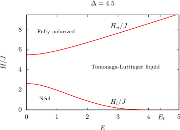
Figure 1: (Color online) Ground-state phase diagram of the $S\!=\!1/2$ XXZ-chain (5) for $\Delta=4.5$ in the $(E,H/J)$-plane. For $E=0$ the phase transitions occur at $H_{l}/J=2.637\ldots$ and $H_{u}/J=\Delta+1=5.5$. For $E>E_{l}$ there does not exist any Néel ordering.

III Results

III.1 Free-fermion case

As known, in case of zero anisotropy $\Delta=0$, the $S\!=\!1/2$ XXZ-chain reduces to the much simpler XX-chain which, in turn, can be solved exactly by mapping it onto a free-fermion system by means of the Jordan-Wigner transformation.JW The XX-chain with DM-term is also exactly solvable within this context.der06a ; der06b ; der00 ; der99 Thus, starting with the Hamiltonian (5) with $\Delta=0$ and performing a Jordan-Wigner transformation to free fermions:

$$S_{n}^{+} =\prod_{j=1}^{n-1}\left(1-2c_{j}^{+}c_{j}\right)c_{n}^{+}\,,$$ (15a)

$$S_{n}^{-} =\prod_{j=1}^{n-1}\left(1-2c_{j}^{+}c_{j}\right)c_{n}\,,$$ (15b)

$$S_{n}^{z} =c_{n}^{+}c_{n}-1/2\,,$$ (15c)

where $c_{n}^{+}$ and $c_{n}$ are creation and annihilation operators of spinless fermions obeying the standard anti-commutation relations, $\left\{c_{n},c_{m}\right\}=0$, $\left\{c_{n}^{+},c_{m}\right\}=\delta_{nm}$, one arrives at the following free-fermion Hamiltonian:

$$\mathcal{H}_{\text{XX-DM}} =\frac{NH}{2}-H\sum_{n=1}^{N}c_{n}^{+}c_{n}$$ (16)

$$\ +\frac{J}{2}\sum_{n=1}^{N}\left(\left(1+iE\right)c_{n}^{+}c_{n+1}+\left(1-iE\right)c_{n+1}^{+}c_{n}\right)\,.$$

Here, as usual, periodic boundary conditions are assumed. Then, the Fourier transform diagonalizes the Hamiltonian and yields

$$\mathcal{H}_{\text{XX-DM}} =\sum_{k}\varepsilon_{k}\left(c_{k}^{+}c_{k}-1/2\right)\,,$$ (17a)

$$\varepsilon_{k} =-H+J\left(\cos{k}+E\sin{k}\right)\,.$$ (17b)

For the free-fermion picture of the model under consideration, one can easily obtain all thermodynamic functions in the thermodynamic limit in the form of integrals over the one-dimensional Brillouin zone, $k\in\left[-\pi,\pi\right]$ (see for example Ref. [der12, ]). So, one gets for the free energy $f$ per spin, the magnetization $M$, the polarization $P$ and the magnetoelectric tensor $\alpha$:

$$f(T,H,E) =\frac{1}{2\pi}\int_{-\pi}^{\pi}\left(\frac{\varepsilon_{k}}{2}+T\log(n_{k})\right){\rm d}k\,,$$ (18a)

$$M(T,H,E) =\frac{1}{2\pi}\int_{-\pi}^{\pi}(n_{k}-1/2)\,{\rm d}k\,,$$ (18b)

$$P(T,H,E) =-\frac{1}{2\pi}\int_{-\pi}^{\pi}(n_{k}-1/2)\sin{k}\,{\rm d}k\,,$$ (18c)

$$\alpha(T,H,E) =-\frac{1}{2\pi T}\int_{-\pi}^{\pi}n_{k}(1-n_{k})\sin{k}\,{\rm d}k\,,$$ (18d)

where $n_{k}=1/(1+e^{\varepsilon_{k}/T})$ are the occupation numbers of spinless fermions.

Figure 2 shows the dependence of the magnetization $M$ and the polarization $P$ on the magnetic field $H$ for different values of the electric field $E$ in units of $J$ and for very low temperature. The phase transitions at the corresponding values of $H=H_{u}=\sqrt{1+E^{2}}$ can be observed. All critical exponents are $1/2$. The curves in Fig. 2 are obtained by the method described in the next section and in App. A, see for instance Eqs. (19) and (21). Similarly, direct numerical calculation of the same quantities by computing the integrals on the r. h. s. of Eqs. (18) produce data with deviations smaller than $10^{-6}$.

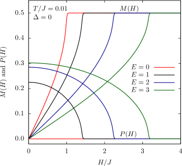
Figure 2: (Color online) Magnetization $M$ and polarization $P$ as functions of the magnetic field $H$ for anisotropy $\Delta=0$, temperature $T/J=0.01$ and different values of the electric field $E=0,1,2,3$.

III.2 General case

It is convenient to express the magnetization and the polarization in terms of static short-range correlation functions of the XXZ-chain. Using Eqs. (11a), (12b), and (13) as well as the translational invariance of the Hamiltonian (8) one obtains

$$M(T,H,E) =\langle S_{1}^{z}\rangle\,,$$ (19a)

$$P(T,H,E) =-\frac{E}{\sqrt{1+E^{2}}}\langle S_{1}^{x}S_{2}^{x}+S_{1}^{y}S_{2}^{y}\rangle\,.$$ (19b)

Due to recent progress in the theory of integrable models static short-range correlation functions of the XXZ-chain can be calculated exactly. It can be shown that all static correlation functions of the one-dimensional XXZ-model can be expressed as polynomials in the derivatives of three functionsJimbo et al. (2009) $\varphi$, $\omega$, and $\omega^{\prime}$ which are determined by solutions of certain numerically well behaved linear and non-linear integral equations.Boos and Göhmann (2009) In App. A we give the definitions of these functions in the massive case $\widetilde{\Delta}>1$.Trippe et al. (2010) In the critical case $0\leq\widetilde{\Delta}<1$ the definitions are quite similar.Boos et al. (2008)

Employing the short-hand notations

$$\varphi_{(n)} =\partial_{x}^{n}\varphi(x)|_{x=0}\,,$$ (20a)

$$f_{(m,n)} =\partial_{x}^{m}\partial_{y}^{n}f(x,y)|_{x=y=0}\quad\text{for}\ f=\omega,\omega^{\prime}\,,$$ (20b)

we obtainTrippe et al. (2010)

$$\langle S_{1}^{z}\rangle =-\frac{1}{2}\varphi_{(0)}\,,$$ (21a)

$$\langle S_{1}^{x}S_{2}^{x}\rangle =\langle S_{1}^{y}S_{2}^{y}\rangle=\ -\frac{\omega_{(0,0)}}{8\operatorname{sh}{\eta}}-\frac{\operatorname{ch}{\eta}\ \omega^{\prime}_{(1,0)}}{8\eta}\,,$$ (21b)

where the parameter $\eta$ is defined by $\widetilde{\Delta}=\operatorname{ch}{\eta}$ for $\widetilde{\Delta}>1$, i. e. $E<\sqrt{\Delta^{2}-1}$. Similar expressions can be obtained for the case $0\leq\widetilde{\Delta}<1$,Boos et al. (2008) i. e. $E>\sqrt{\Delta^{2}-1}$.

Combining Eqs. (21), (19), and (12c) the magnetization, the polarization and thereby the magnetoelectric tensor can be calculated exactly for all temperatures over the whole range of the phase diagram Fig. 1.

By solving the linear and non-linear integral equations of Appendix A, the MEE parameters $M$, $P$ and $\alpha$ of Eqs. (19a), (19b) and (12c), respectively, can be calculated with high numerical accuracy.

Figure 3 shows these three quantities as functions of the magnetic field for very low temperatures and different values of the electric field. The phase transitions at the corresponding values of the magnetic field (see Fig. 1) can be easily observed. Interestingly, in the Tomonaga-Luttinger liquid phase, the electric polarization $P$ is a non-monotonic function of the magnetic field $H$ whereas it is constant, $P\neq 0$, in the Néel-ordered phase and vanishing in the fully polarized ferromagnetic phase. Here, the critical exponents characterizing the magnetic field dependence of the electric polarization in the vicinity of critical values of the magnetic field, $H=H_{l}(E)$ and $H=H_{u}(E)$, are all equal to $1/2$,

$$P \sim\left(H-H_{l}\right)^{1/2}\,,$$ (22a)

$$P \sim\left(H_{u}-H\right)^{1/2}\,.$$ (22b)

This can be also observed by the van Hove-like singularities of the magnetoelectric tensor $\alpha(H)$. We evaluated the magnetoelectric tensor $\alpha(T,H,E)$ by numerical derivatives of $P$ and $M$ with respect to $H$ and $E$, respectively (see Eqs. (1) or (12c)). In the inset of Fig. 3 it is shown that both data sets coincide.

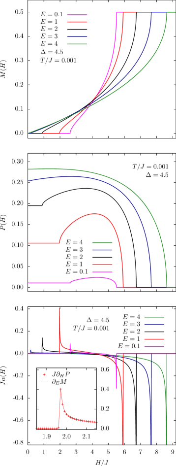
Figure 3: (Color online) Magnetization $M$, polarization $P$, and magnetoelectric tensor $\alpha$ as functions of the magnetic field $H$ for anisotropy $\Delta=4.5$, temperature $T/J=0.001$ and different values $E=0.1,1,2,3,4$. In the inset of the third panel the two data sets $J\partial_{H}P$ and $\partial_{E}M$ are compared, both obtained numerically using the five-point stencil algorithm of the first derivative.

Figure 4 illustrates the temperature-driven melting of the singularity of the magnetoelectric tensor as function of the magnetic field. The values $E=1$ of the electric field and $T=0.001\,J$ of the temperature belong to the red curve of the third panel of Fig. 3. With increasing temperature the curve becomes more and more flat. Note that the temperature in Fig. 4 is only slightly increased. For $T=0.03\,J\ll J$, for instance, there is no longer any indication of singular behavior. The two curves $J\partial_{H}P$ and $\partial_{E}M$ would overlay exactly such that only one of them is shown.

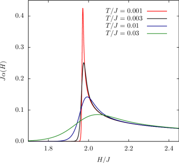
Figure 4: (Color online) Temperature dependence of the magnetoelectric tensor $\alpha$ for $E=1$ and $\Delta=4.5$ close to the critical point $H\approx 1.95J$. The square-root singularity for $T=0$ decays rapidly with increasing temperature.

In Figure 5 the temperature dependence of the electric polarization and the magnetoelectric tensor are displayed. The values of the electric and magnetic field are chosen in a way such that the different ground-state phases are represented (see Fig. 1), just below and above the critical lines. All curves show non-monotonic behavior and go to zero in the infinite-temperature limit. In the zero-temperature limit the magnetoelectric tensor vanishes in the Néel-ordered and in the fully polarized ferromagnetic phase, whereas it remains constant in the Tomonaga-Luttinger liquid.

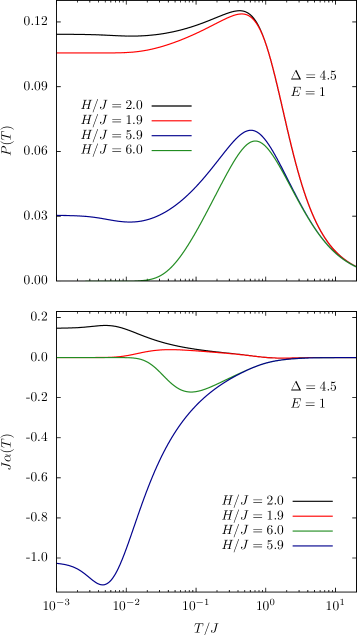
Figure 5: (Color online) Temperature dependence of the electric polarization $P$ and the magnetoelectric tensor $\alpha$ close to the critical points $H/J\approx 1.95$ and $H/J=4.5+\sqrt{2}$ (see Fig. 1).

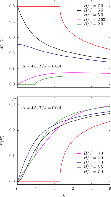
Figure 6: (Color online) Electric field dependence of the magnetization $M$ and the polarization $P$ for different fixed values of the magetic field $H$ at very low temperature $T/J=0.001$. The values $H/J=2.637$ and $H/J=5.5$ correspond to the phase transitions from the Néel-ordered ground state to the Tomonaga-Luttinger liquid and from the Tomonaga-Luttinger liquid to the fully polarized ferromagnetic state, respectively (see Fig. 1).

Figure 6 shows the dependence of the magnetization $M$ and the polarization $P$ on the electric field $E$ for fixed values of the magnetic field $H$, again for very low temperatures. For higher temperatures the cusps smooth out. Phase transitions only occur in the regimes (see Fig. 1 with $\Delta=4.5$)

$$H/J<H_{l}(E=0)/J =2.637\ldots\,,$$ (23a)

$$H/J>H_{u}(E=0)/J =\Delta+1=5.5\,.$$ (23b)

Here, the singularities are described by three different exponents. In most cases one can observe square-root behavior. This is always the case for the magnetization. However, for the special value of magnetic field $H/J=1+\Delta$, which corresponds to the transition from the Tomonaga-Luttinger liquid phase to the fully polarized ferromagnetic phase at zero electric field, the electric polarization grows quadratically in $E$.

This can be explained as follows. The critical behavior of the correlation function $\langle S_{1}^{x}S_{2}^{x}\rangle$ for fixed $E$ as function of the magnetic field $H$ is $\langle S_{1}^{x}S_{2}^{x}\rangle\sim\sqrt{H_{u}-H}$ for $H\leq H_{u}$. The gap between the fixed value $H=\Delta+1$ and $H_{u}(E)=\Delta+\sqrt{1+E^{2}}$ is quadratic in $E$. Therefore, the critical behavior is $\sqrt{H_{u}-H}\sim E$. Due to the prefactor in Eq. (19b) one eventually obtains

$$P(E)\Big{|}_{H=\Delta+1}=-\frac{2E}{\sqrt{1+E^{2}}}\langle S_{1}^{x}S_{2}^{x}\rangle\Big{|}_{H=\Delta+1}\sim E^{2}\,.$$ (24)

In addition to that, the polarization as a function of the external electric field can also exhibit linear behavior with further transition to the square-root form, at the values of $E$ corresponding to the transition from the Néel-ordered phase to the Tomonaga-Luttiger liquid phase. Thus, one can define the critical exponent $\delta_{E}$ which characterizes the behavior of the polarization on its corresponding conjugate field (electric field),

$$P\sim|E-E_{c}|^{\delta_{E}},\qquad\delta_{E}=1/2,1,2\,.$$ (25)

The limiting value of $P(E)$ for $E\to\infty$ can also be understood. Due to Eqs. (8) and (10) the model reduces in this limit to a free-fermion model with $H\to 0$. The rescaling $\widetilde{J}\mapsto J$ yields

$$\mathcal{H}\mapsto J\sum_{n=1}^{N}\left(S_{n}^{x}S_{n+1}^{x}+S_{n}^{y}S_{n+1}^{y}\right)\,.$$ (26)

Then, the free energy per lattice site follows from Eq. (18a) and is given by

$$f(T,H,E)=-\frac{T}{\pi}\int_{0}^{\pi}\log\left[2\,\text{cosh}{\left(\frac{J\cos{k}}{2T}\right)}\right]\,{\rm d}k\,.$$ (27)

Hence, the partition function $Z=\operatorname{tr}{({\rm e}^{-H/T})}={\rm e}^{-F/T}$ with $f=F/N$ and the nearest-neighbor correlation functions can be calculated in the low-temperature limit,

$$\langle S_{1}^{x}S_{2}^{x}\rangle= -\frac{T}{2N}\frac{\partial\log{(Z)}}{\partial J}=\frac{1}{2}\frac{\partial f}{\partial J}$$

$$= -\frac{1}{4\pi}\int_{0}^{\pi}\tanh{\left(\frac{J\cos{k}}{2T}\right)}\cos{k}\,{\rm d}k$$

$$\xrightarrow{\makebox[17.07164pt][c]{\tiny$\!T\!\!\to\!0$}} -\frac{1}{4\pi}\int_{0}^{\pi}|\cos{k}|\,{\rm d}k=-\frac{1}{2\pi}\,.$$ (28)

Therefore, $P(E)\to 1/\pi$ for $E\to\infty$ and $T\to 0$.

IV Discussions and Conclusion

The system considered in the present paper, being an integrable one, allowed us to obtain an exact description of the MEE by means of QTM and NLIE techniques. We considered a microscopic dielectric polarization to be proportional to the antisymmetric product of $x$- and $y$-components of the spins from two adjacent sites, i. e. to a spin current $j^{z}$. This mechanism, which is known as a KNB-mechanism,KNB is realized in several one-dimensional magnetic materials.KNB_exp1 ; KNB_exp2 ; KNB_exp3 ; KNB_exp4 ; J1J2_1 ; J1J2_2 ; J1J2_3 ; J1J2_4 ; J1J2_5 ; J1J2_6 ; J1J2_7 In our model, however, we have to impose a restriction in order to preserve integrability. While the standard model to describe the MEE in one-dimensional magnetic materials with KNB-mechanism is the $J_{1}$-$J_{2}$-chain, Eq. (4), we consider an ordinary XXZ-chain in a magnetic field with DM-terms, Eq. (5). The DM-terms describe a local dielectric polarization where the corresponding coefficient is the electric field magnitude $E$ in appropriate units.

The main objects of our investigation are the magnetization $M$ and the dielectric polarization $P$, which are the thermal averages of the operators $\sum_{n=1}^{N}S_{n}^{z}$ and $\sum_{n=1}^{N}(S_{n}^{y}S_{n+1}^{x}-S_{n}^{x}S_{n+1}^{y})$, respectively. As a main result the exact finite-temperature plots of $M(T,H,E)$ and $P(T,H,E)$ have been obtained, especially in the low-temperature regime. Below we summarize the most interesting features of these plots.

As we mapped the system with DM-interaction onto the ordinary XXZ-chain, where $E$ enters the effective coupling constant $\widetilde{J}(E)$ and effective anisotropy $\widetilde{\Delta}(E)$, the magnetization curves $M(H)$ at fixed values of $T$ and $E$ (see Fig. 3, upper panel) do not show any great difference from those of the conventional XXZ-chain.qtm4 The polarization as a function of magnetic field at constant values of temperature and electric field exhibits non-monotonic behavior (see Fig. 3, middle panel).

Since we chose a large anisotropy $\Delta=4.5$, one can distinguish three possible parts of the polarization curve corresponding to the Néel-ordered phase, Tomonaga-Luttinger massless regime, and fully polarized spin configuration of the effective XXZ-chain, respectively. All these three regimes are easily recognizable in the middle panel of Fig. 3. At low values of $H$, when the system is in the Néel-ordered ground state, the polarization $P(H)$ is constant and thus starts with a plateau. One can also observe the effect of the electric field on the polarization $P(H)$. With increasing value of $E$ the plateau becomes shorter and higher. In the limit $E\rightarrow\infty$ the effective anisotropy parameter $\widetilde{\Delta}=1/\sqrt{1+E^{2}}$ becomes zero, which means $M=0$ and $P=P_{max}=1/\pi$ for $H=0$. The second segment of the magnetic field dependent polarization corresponds to the Tomonaga-Luttinger regime of the effective XXZ-chain. This part of the polarization curve is a dome which starts at the plateau and ends at the value $P=0$ corresponding to the fully polarized ground state of the spin system. The values of the critical exponents corresponding to the two critical values of $H$ (transitions from the Néel-ordered ground state to the Tomonaga-Luttinger regime and from the Tomonaga-Luttinger regime to the fully polarized spin state) are equal to $1/2$.

A feature of the model under consideration is the vanishing polarization $P(H)$ at $E=0$. There only exists mutual influence of electric and magnetic properties of the model for $E\neq 0$. With respect to the electric properties the system does not show ferroic order, but is a conventional ‘dielectric’ system which acquires polarization in an external electric field. However, this dielectric polarization is strongly affected by the external magnetic field as well, which is the MEE one can observe in our system.

Looking at the dependence of the magnetoelectric tensor $\alpha$ on the magnetic field $H$ (see Fig. 3, lower panel) one can easily identify the zero-temperature phase transitions between Néel, Tomonaga-Luttinger and fully polarized ground states by the singular peaks. For sufficiently large $H$ the polarization is zero due to the transition to the fully polarized ferromagnetic state. The magnetoelectric tensor has a negative peak at this transition point. In addition to that, the absolute magnitude of this peak is larger than that of the positive peak corresponding to the transition from the Néel-ordered to the Tomonaga-Luttinger liquid state. This indicates a more dramatic drop of polarization for upper critical magnetic fields compared to its rise for the lower critical fields. However, the type of singularity in both cases is the same with critical exponent equal to 1/2, i. e. $\alpha\sim\left|H-H_{c}\right|^{-1/2}$.

The behavior of the polarization as function of electric field is strongly affected by the magnetic field (see Fig. 6, lower panel). Even at vanishing magnetic field it exhibits non-trivial behavior during the whole process of polarization. The polarization increases linearly for small values of $E$ followed by a smooth curve approaching its saturated value $1/\pi$ in the limit $E\to\infty$. Switching on a magnetic field causes essential changes in the course of the polarization curve. For low magnetic fields the polarization starts linearly as in the $H=0$ case, but changes to a square-root behavior at the value of $E$ corresponding to the transition from Néel-ordered ground state to Tomonaga-Luttinger liquid phase. At this point the polarization curve has a cusp. For intermediate values of the magnetic field the system starts with a Tomonaga-Luttinger liquid phase, and the increase of $E$ does not drive the system to another ground state. One can observe monotonic increase of the polarization with linear behavior at small $E$. At the special value of $H$ corresponding to the critical value of the transition between Tomonaga-Luttinger liquid phase and fully polarized spin configuration at $E=0$, i. e. $H=(\Delta+1)J$, one gets quadratic behavior for small $E$. Finally, for sufficiently large magnetic fields, when the system starts at the fully polarized magnetic configuration, the electric polarization vanishes. This changes dramatically to a square-root increase at the point of quantum phase transition to Tomonaga-Luttinger liquid state. To summarize one can distinguish four different behaviors of the polarization $P(E)$: linear followed by a cusp for $0<H<H_{l}$, linear with a smooth increase for $H=0$ or $H_{l}\leq H<H_{u}$, quadratic for $H=H_{u}$, and vanishing followed by a cusp for $H>H_{l}$.

Finally, the temperature dependencies of the polarization $P$ and of the magnetoelectric tensor $\alpha$ illustrate another interesting feature (see Fig. 5). In the vicinity of quantum critical points the temperature dependence of the polarization is non-monotonic. The most intriguing feature shows the curve for $H=6J$ and $E=1$, where at low temperatures polarization is absent ($P=0$). Then, at intermediate temperatures the polarization curve rises up to values of about $0.065$. Eventually, it drops to zero for high temperatures. Thus, starting from zero temperature and increasing it continuously, the system exhibits a broad polarization peak over almost five orders of magnitude. Here, the values of magnetic and electric fields correspond to the fully polarized ferromagnetic phase just above the critical line. The temperature dependence of the magnetoelectric tensor, which is presented in the lower panel of Fig. 5, is also non-monotonic and indicates the different regimes of the system response.

Although the system considered in the present paper exhibits MEE and also demonstrates a number of interesting features like many regimes of polarization and a thermally activated peak, it does not exhibit ferroelectric polarization, which means that $P$ is always zero, unless $E\neq 0$. In order to obtain more interesting and richer features like double ferroic order or induction of polarization only by the magnetization and/or by the magnetic field within the KNB-mechanism, one should consider more sophisticated models. One way which seems straightforward to us is to include microscopic interactions between local order parameters, e. g. local magnetization and local polarization. One example is

$$\mathcal{H}_{int}\sim\sum_{n=1}^{N}\left(S_{n}^{x}S_{n+2}^{y}-S_{n}^{y}S_{n+2}^{x}\right)S_{n+1}^{z}\,.$$ (29)

The local polarization is composed according to KNB-mechanism and includes next-to-nearest-neighbor spin interactions. Three-site interactions recently received considerable attention in a bit diverse context.der12 ; Suz71 ; Got99 ; Lou04 ; Kro08 ; Der09 It was shown by Suzuki in Ref. [Suz71, ] that there is a series of spin chains with multiple-site interactions of special kind, which can be mapped onto free spinless fermions via the Jordan-Wigner transformation. Unfortunately, the $S\!=\!1/2$ XXZ-chain with three-site spin-interaction terms given by Eq. (29) is no longer integrable. One has to restrict oneself to the XY-chain with corresponding termsder12 ; Suz71 ; Got99 ; Lou04 ; Kro08 ; Der09 or has to implement numerical simulations. Another obvious non-trivial choice of local interaction between magnetization and polarization is $\sum_{n=1}^{N}p_{n}m_{n+1}$. However, in this case even the corresponding XX-model is not exactly solvable.

Another possibility to construct the model exhibiting the double ferroic order and MEE within the integrable systems is to consider rather sophisticated spin chains with special three-spin interaction discussed in Ref. [zvy03, ]. These models seem to be very promising by means of the MEE because of the local interaction between microscopic magnetic and dipole moments presented in their Hamiltonians (if one supposes that the KNB mechanism is realized in the system). This argument allows us to hope that the model could possess a ferroelectric phase generated by the magnetic field solely. All these ideas conveyed above could be the guide line to further developments in the MEE and multiferroics of integrable systems.

V Acknowledgements

The authors thank Jesko Sirker, Temo Vekua, Oleg Derzhko, Alexander Nersesyan and Frank Göhmann for comments and stimulating discussions. V. O. expresses his gratitude to the Department of Theoretical Physics of the Bergische Universität Wuppertal for warm hospitality during the work on this paper. His research stay has been supported by DFG (Grant No. KL 645/8-1). V. O. also likes to acknowledge partial financial support from Volkswagen Foundation (Grant No. I/84 496) and from the project SCS-BFBR 11RB-001. M. B. likes to acknowledge financial support by the DFG (Grant No. KL 645/7-1).

Appendix A Exact determination of correlation functions

The functions $\varphi$, $\omega$, and $\omega^{\prime}$ that determine all static correlation functions of the XXZ-chain are defined in terms of solutions of linear and non-linear integral equations. They were termed the physical part of the problem,Boos and Göhmann (2009) since the physical parameters like temperature or magnetic field enter solely through these functions. We provide their definitions only for the case $\widetilde{\Delta}>1$. The definitions for the case $-1<\widetilde{\Delta}<1$ can be found in Ref. [Boos et al., 2008].

First of all let us define a basic pair of auxiliary functions as the solution of the non-linear integral equationsTrippe et al. (2010)

$$\log\mathfrak{b}(x) =-\frac{2\widetilde{J}\operatorname{sh}(\eta)}{T}d(x)-\frac{H}{2T}+\kappa\ast\log\left(1+\mathfrak{b}\right)(x)-\kappa^{-}\ast\log\left(1+\overline{\mathfrak{b}}\right)(x)\,,$$ (30a)

$$\log\overline{\mathfrak{b}}(x) =-\frac{2\widetilde{J}\operatorname{sh}(\eta)}{T}d(x)+\frac{H}{2T}+\kappa\ast\log\left(1+\overline{\mathfrak{b}}\right)(x)-\kappa^{+}\ast\log\left(1+\mathfrak{b}\right)(x)\,,$$ (30b)

where we denote with $\ast$ the convolution $(f\ast g)(x)=\frac{1}{\pi}\int\nolimits_{-\pi/2}^{\pi/2}f(x-y)g(y){\rm d}y$. Here we introduced the parameter $\eta$ defined by $\widetilde{\Delta}=\operatorname{ch}(\eta)$. Eqs. (30) are valid for all $\eta\geq 0$ meaning that $\widetilde{\Delta}>1$. The driving term $d$ is given by its Fourier series,

$$d(x)=\sum_{k=-\infty}^{\infty}\frac{{\rm e}^{2ikx}}{\operatorname{ch}(\eta k)}\,.$$ (31)

Note that the physical parameters temperature $T$, magnetic field $H$, and coupling $\widetilde{J}$ enter only through the driving terms of Eqs. (30) into our formulae. The kernels $\kappa$ and $\kappa^{\pm}$ are given by

$$\kappa(x) =\sum_{k=-\infty}^{\infty}\frac{{\rm e}^{-\eta|k|+2imkx}}{2\operatorname{ch}(\eta k)}\,,$$ (32a)

$$\kappa^{\pm}(x) =\kappa(x\pm i\eta^{-})\,,$$ (32b)

where $\eta^{-}=\eta-\epsilon$ with an arbitrary small number $\epsilon>0$.

Except for the auxiliary functions $\mathfrak{b}$ and $\overline{\mathfrak{b}}$ we need two more pairs of functions $g_{\mu}^{(\pm)}$ and ${g^{\prime}}_{\mu}^{(\pm)}$ in order to define $\varphi$, $\omega$, and $\omega^{\prime}$. Both pairs satisfy linear integral equations involving $\mathfrak{b}$ and $\overline{\mathfrak{b}}$,

$$g^{+}_{\nu}(x)=-d(x-\nu)+\kappa\ast\frac{g^{+}_{\nu}}{1+\mathfrak{b}^{-1}}(x)-\kappa^{-} \ast\frac{g^{-}_{\nu}}{1+\overline{\mathfrak{b}}^{-1}}(x)\,,$$ (33a)

$$g^{-}_{\nu}(x)=-d(x-\nu)+\kappa\ast\frac{g^{-}_{\nu}}{1+\overline{\mathfrak{b}}^{-1}}(x)-\kappa^{+} \ast\frac{g^{+}_{\nu}}{1+\mathfrak{b}^{-1}}(x)\,,$$ (33b)

$${g^{\prime}}^{+}_{\nu}(x)=-c_{+}(x-\nu)+\kappa\ast\frac{{g^{\prime}}^{+}_{\nu}}{1+\mathfrak{b}^{-1}}(x)-\kappa^{-} \ast\frac{{g^{\prime}}^{-}_{\nu}}{1+\overline{\mathfrak{b}}^{-1}}(x)+\ l\ast\frac{g^{+}_{\nu}}{1+\mathfrak{b}^{-1}}(x)-l^{-}\ast\frac{g^{-}_{\nu}}{1+\overline{\mathfrak{b}}^{-1}}(x)\,,$$ (33c)

$${g^{\prime}}^{-}_{\nu}(x)=-c_{-}(x-\nu)+\kappa\ast\frac{{g^{\prime}}^{-}_{\nu}}{1+\overline{\mathfrak{b}}^{-1}}(x)-\kappa^{+} \ast\frac{{g^{\prime}}^{+}_{\nu}}{1+\mathfrak{b}^{-1}}(x)+\ l\ast\frac{g^{-}_{\nu}}{1+\overline{\mathfrak{b}}^{-1}}(x)-l^{+}\ast\frac{g^{+}_{\nu}}{1+\mathfrak{b}^{-1}}(x)\,.$$ (33d)

The functions $l$ and $c_{\pm}$ are again given by their Fourier series,

$$l(x)=\sum_{k=-\infty}^{\infty}\frac{\operatorname{sign}(k){\rm e}^{2ikx}}{4\operatorname{ch}^{2}(\eta k)}\,,\quad\ l^{\pm}(x)=l(x\pm i\eta^{-})\,,\quad\ c_{\pm}(x)=\pm\sum_{k=-\infty}^{\infty}\frac{{\rm e}^{\pm\eta k+2ikx}}{2\operatorname{ch}^{2}(\eta k)}\,,$$ (34)

where we set $\operatorname{sign}(0)=0$ for the sign function.

The functions $\varphi(\mu)$, $\omega(\mu_{1},\mu_{2})$, and $\omega^{\prime}(\mu_{1},\mu_{2})$ that determine the explicit form of the correlation functions of the XXZ-chain can be written as integrals involving $\mathfrak{b}$, $\overline{\mathfrak{b}}$, $g_{\mu}^{(\pm)}$, and ${g^{\prime}}_{\mu}^{(\pm)}$. The function

$$\varphi(\nu) =\frac{1}{2\pi}\int\nolimits_{-\pi/2}^{\pi/2}\left(\frac{g_{\widetilde{\nu}}^{-}(x)}{1+\overline{\mathfrak{b}}(x)^{-1}}-\frac{g_{\widetilde{\nu}}^{+}(x)}{1+\mathfrak{b}(x)^{-1}}\right){\rm d}x\,,$$ (35a)

determines the magnetization $$M(T,H)=-{\textstyle\frac{1}{2}}\varphi(0)$$ which is the only independent one-point function of the XXZ-chain. The function

$$\omega(\nu_{1},\nu_{2}) =-4\kappa(\widetilde{\nu}_{2}-\widetilde{\nu}_{1})+\widetilde{K}_{\eta}(\widetilde{\nu}_{2}-\widetilde{\nu}_{1})-d\ast\left(\frac{g_{\widetilde{\nu}_{1}}^{+}}{1+\mathfrak{b}^{-1}}+\frac{g_{\widetilde{\nu}_{1}}^{-}}{1+\overline{\mathfrak{b}}^{-1}}\right)(\widetilde{\nu}_{2})\,,$$ (35b)

also determines the energy per lattice site of the XXZ-chain, $$\langle s_{j-1}^{x}s_{j}^{x}+s_{j-1}^{y}s_{j}^{y}+\Delta s_{j-1}^{z}s_{j}^{z}\rangle=\operatorname{sh}(\eta)\omega(0,0)/4 \omega^{\prime}(\mu_{1},\mu_{2})$$. The function is defined as

$$\frac{\omega^{\prime}(\nu_{1},\nu_{2})}{\eta} =-4l(\widetilde{\nu}_{2}-\widetilde{\nu}_{1})+\widetilde{L}_{\eta}(\widetilde{\nu}_{2}-\widetilde{\nu}_{1})-d\ast\left(\frac{{g^{\prime}}_{\widetilde{\nu}_{1}}^{+}}{1+\mathfrak{b}^{-1}}+\frac{{g^{\prime}}_{\widetilde{\nu}_{1}}^{-}}{1+\overline{\mathfrak{b}}^{-1}}\right)(\widetilde{\nu}_{2})$$

$$\mspace{200.0mu}-c_{-}\ast\frac{g_{\widetilde{\nu}_{1}}^{+}}{1+\mathfrak{b}^{-1}}(\widetilde{\nu}_{2})-c_{+}\ast\frac{g_{\widetilde{\nu}_{1}}^{-}}{1+\overline{\mathfrak{b}}^{-1}}(\widetilde{\nu}_{2})\,,$$ (35c)

where we set $\widetilde{\nu}=-i\nu$ and $\widetilde{\nu}_{j}=-i\nu_{j}$. The functions $\widetilde{K}_{\eta}$ and $\widetilde{L}_{\eta}$ are determined by

$$\widetilde{K}_{\eta}(x) =\frac{\operatorname{sh}(2\eta)}{2\sin(x+i\eta)\sin(x-i\eta)}\,,$$ (36a)

$$\widetilde{L}_{\eta}(x) =\frac{i\sin(2x)}{2\sin(x+i\eta)\sin(x-i\eta)}\,.$$ (36b)

For the calculation of the magnetization and the polarization, the non-linear integral equations for $\mathfrak{b}$ and $\overline{\mathfrak{b}}$ as well as their linear counterparts for $g_{\mu}^{(\pm)}$ and ${g^{\prime}}_{\mu}^{(\pm)}$ were solved iteratively in Fourier space utilizing the fast Fourier transformation algorithm. The derivatives of $g_{\mu}^{(\pm)}$ and ${g^{\prime}}_{\mu}^{(\pm)}$ with respect to $\mu$, needed in the computation of the derivative of $\omega^{\prime}$ satisfy linear integral equations as well, which were obtained as derivatives of the equations for $g_{\mu}^{(\pm)}$ and ${g^{\prime}}_{\mu}^{(\pm)}$. Taking into account derivatives is particularly simple in Fourier space.

References

- (1) A. R. Akbashev and A. R. Kaul, Russ. Chem. Rev. 80, 1159 (2011).
- (2) K. Wang, J.-M. Liu and Z. Ren, Adv. Phys. 58, 321 (2009).
- (3) S.-W. Cheong and M. Mostovoy, Nature Materials 6, 13 (2007).
- (4) M. Fiebig, J.Phys.D: Appl. Phys. 38, R123 (2005).
- (5) C. Jia and J. Berakdar, Appl. Phys. Lett. 95, 012105 (2009).
- (6) H. Katsura, N. Nagaosa, and A. V. Balatsky, Phys. Rev. Lett. 95, 057205 (2005).
- (7) I. A. Sergienko and E. Dagotto, Phys. Rev. B 73, 094434 (2006).
- (8) C. L. Jia, S. Onoda, N. Nagaosa, and J.-H. Han, Phys. Rev. B 76, 144424 (2007).
- (9) M. Mostovoy, Phys. Rev. Lett. 96, 067601 (2006).
- (10) T. A. Kaplan and S. D. Mahanti, Phys. Rev. B 83, 174432 (2011).
- (11) T. Kimura, T. Goto, H. Shintani, K. Ishizaka, T. Arima, and Y. Tokura, Nature(London) 426, 55 (2003).
- (12) T. Goto, T. Kimura, G. Lawes, A. P. Ramirez, and Y. Tokura, Phys. Rev. Lett. 92, 257201 (2004).
- (13) G. Lawes, A. B. Harris, T. Kimura, N. Rogado, R. J. Cava, A. Aharony, O. Entin-Wohlman, T. Yildrim, M. Kenzelmann, C. Broholm, and A. P. Ramirez, Phys. Rev. Lett. 95, 087205 (2005).
- (14) K. Taniguchi, N. Abe, T. Takenobu, Y. Iwasa, and T. Arima, Phys. Rev. Lett. 97, 097203 (2006).
- (15) S. Seki, Y. Yamasaki, M. Soda, M. Matsuura, K. Hirota, and Y. Tokura, Pshys,. Rev. Lett 100, 127201 (2008).
- (16) S. Park, Y. J. Choi, C. L.Zang, and S.-W. Cheong, Phes. Rev. Lett 98, 057601 (2007).
- (17) A. A. Bush, V. N. Glazkov, M. Hagiwara, T. Kashiwagi, S. Kimura, K. Omura, L. A. Prozorova, L. E. Svistov, A. M. Vasiliev, and A. Zheludev, Phys. Rev. B 85, 054421 (2012).
- (18) Y. Yasui, Y. Naito, K. Saso, T. Moyoshi, M. Sato, and K. Kakurai, J. Phys. Soc. Jpn 77, 023712 (2008).
- (19) Y. Naito, K. Sato, Y. Yasui, Yu. Kobayashi, Yo. Kobayashi, and M. Sato, J. Phys. Soc. Jpn 76, 023708 (2007).
- (20) F. Schrettle, S. Krohns, P. Lunkenheimer, J. Hemberger, N. Büttgen, H.-A. Krug von Nidda, A. V. Prokofiev, and A. Loidl, Phys. Rev. B 77, 144101 (2008).
- (21) S. Seki, T. Kurumaji, S. Ishiwata, H. Matsui, H. Murakawa, Y. Tokunaga, Y. Kaneko, T. Hasegawa, and Y. Tokura, Phys. Rev. B 82, 064424 (2010).
- (22) M. Arlego, F. Heidrich-Meisner, A. Honecker, G. Rossini, and T. Vekua, Phys. Rev. B 84, 224409 (2011).
- (23) D. V. Dmitriev, V. Ya. Krivnov, and N. Yu. Kuzminyh, Phys. Rev. B 84, 214438 (2011).
- (24) A. U. B. Wolter, F. Lipps, M. Sch pers, S.-L. Drechsler, S. Nishimoto, R. Vogel, V. Kataev, B. B chner,H. Rosner, M. Schmitt, M. Uhlarz, Y. Skourski, J. Wosnitza, S. S llow, K. C. Rule, Phys. Rev. B 85, 014407 (2012).
- (25) A. K. Kolezhuk, F. Heidrich-Meisner, S. Greschner, and T. Vekua, Phys. Rev. B 85, 064420 (2012).
- (26) J. Ren and J. Sirker, Phys. Rev. B 85, 140410 (2012).
- (27) J. Sirker, Phys. Rev. B 81, 014419 (2010).
- (28) C. Jia and J. Berakdar, arXiv:1101.2067 (unpublished).
- (29) A. Klümper, Eur. Phys. J. B 5, 677 (1998).
- (30) A. Klümper, Lect. Notes in Phys. 645, 349 (2004).
- (31) J. Damerau, A. Klümper, J. Stat. Phys.: Theor and Exp. 12, 12014 (2006).
- (32) A. Seel, T. Bhattacharyya, F. Göhmann, A. Klümper, J. Stat. Mech.: Theor. and Exp 08, 08030 (2007)
- (33) C. Trippe, A. Klümper, LTP 33, 920 (2007).
- (34) G. A. P. Ribeiro, A. Klümper, Nucl. Phys. B 801, 247 (2008).
- (35) C. Trippe, A. Honecker, A. Klümper, and V. Ohanyan, Phys. Rev. B 81, 054402 (2010).
- (36) F. C. Alcaraz and W. F. Wreszinski, J. Stat. Phys. 58, 45 (1990).
- (37) D. N. Aristov, and S. V. Maleyev, Phys. Rev. B 62, R751 (2000).
- (38) R. Jafari and A. Langari, arXiv:0812.1862 (unpublished).
- (39) H. Karimi and I. Affleck, Phys. Rev. B 84, 174420 (2011).
- (40) E. Lieb, T. Schulz, and D. Mattis, Annals of Phys.(N.Y.) 16, 407 (1961).
- (41) O. Derzhko, and T. Verkholyak, J. Phys. Soc. Jpn. 75, 104711 (2006).
- (42) O. Derzhko, T. Verkholyak, T. Krokhmalskii, and H. Büttner, Phys. Rev. B 73, 214407 (2006).
- (43) O. Derzhko, J. Richter, and O. Zaburannyii, J. Phys.: Condens. Matter 12, 8661 (2000).
- (44) O. Derzhko, J. Richter, Phys. Rev. B 59, 100 (1999).
- (45) M. Topilko, T. Krokhmalskii, O. Derzhko, and V. Ohanyan, Eur. Phys. J. B 85, 278 (2012).
- Jimbo et al. (2009) M. Jimbo, T. Miwa, and F. Smirnov, J. Phys. A 42, 304018 (2009).
- Boos and Göhmann (2009) H. Boos and F. Göhmann, J. Phys. A 42, 315001 (2009).
- Trippe et al. (2010) C. Trippe, F. Göhmann, and A. Klümper, Eur. Phys. J. B 73, 253 (2010).
- Boos et al. (2008) H. Boos, J. Damerau, F. Göhmann, A. Klümper, J. Suzuki, and A. Weiße, J. Stat. Mech.: Theor. Exp. P08010 (2008).
- (50) M. Suzuki, Prog. Theor. Phys. 46, 1337 (1971).
- (51) D. Gottlieb and J. Rössler, Phys. Rev. B 60, 9232 (1999).
- (52) P. Lou, W.-C. Wu, and M.-C. Chang, Phys. Rev. B 70, 064405 (2004).
- (53) T. Krokhmalskii, O. Derzhko, J. Stolze, and T. Verkholyak, Phys. Rev. B 77, 174404 (2008).
- (54) O. Derzhko, T. Krokhmalskii, J. Stolze, and T. Verkholyak, Phys. Rev. B 79, 094410 (2009).
- (55) A. A. Zvyagin and A. Klümper, Phys. Rev. B 68, 144426 (2003);H. Frahm and C. Rödenbeck, Eur. Phys. J. B 10, 409 (1999); H. Frahm, J. Phys. A: Math. Gen. 25, 1417 (1992); N. Muramoto and M. Takahashi, J. Phys. Soc. Jpn. 68, 2098 (1999).