Families of building sets and regular wonderful models

Abstract

Given a subspace arrangement, there are several De Concini-Procesi models associated to it, depending on distinct sets of initial combinatorial data (building sets). The first goal of this paper is to describe, for the root arrangements of types $A_{n}$, $B_{n}$ (=$C_{n}$), $D_{n}$, the poset of all the building sets which are invariant with respect to the Weyl group action, and therefore to classify all the wonderful models which are obtained by adding to the complement of the arrangement an equivariant divisor. Then we point out, for every fixed $n$, a family of models which includes the minimal model and the maximal model; we call these models regular models and we compute, in the complex case, their Poincaré polynomials.

1 Introduction

In [3], [4], De Concini and Procesi constructed wonderful models for the complement of a subspace arrangement in a vector space. These are smooth varieties, proper over the given space, in which the union of the subspaces is replaced by a divisor with normal crossings.

The interest in these varieties was at first motivated by an approach to Drinfeld construction of special solutions for Khniznik-Zamolodchikov equation (see [7]). Moreover, in [3] it was shown, using the cohomology description of these models to give an explicit presentation of a Morgan algebra, that the mixed Hodge structure and the rational homotopy type of the complement of a complex subspace arrangement depend only on the intersection lattice (viewed as a ranked poset).

Then real and complex De Concini-Procesi models turned out to play a relevant role in several fields of mathematical research: subspace and toric arrangements, toric varieties and tropical geometry, moduli spaces of curves, configuration spaces, box splines, index theory, discrete geometry (see for instance [5], [6], [8], [9], [11], [21], [22] and [27]).

In general, given a subspace arrangement, there are several De Concini-Procesi models associated to it, depending on distinct sets of initial combinatorial data (building sets, see Section 2.1). Among these building sets there are always a minimal one and a maximal one with respect to inclusion: as a consequence there are always a minimal and a maximal De Concini-Procesi model.

The importance of the minimal construction was immediately pointed out, but real and complex non minimal models (in particular maximal models) appeared in various contexts (see [1], [2], [19], [25]). For instance it is well known that the toric variety of type $A_{n-1}$ is isomorphic to the maximal model associated to the boolean arrangement (see [17] for further references).

In this paper we will deal with the root arrangements of types $A_{n}$, $B_{n}$ (=$C_{n}$), $D_{n}$. As our first goal we will describe, for these arrangements, the poset of all the associated building sets (ordered by inclusion) which are invariant with respect to the Weyl group action, and therefore we will classify all the wonderful models which are obtained by adding to the complement of the arrangement an equivariant divisor.

Our second goal will be to point out, for every fixed $n$, a family of models (which we will call regular models), which includes the minimal model and the maximal model, and to compute the Poincaré polynomials of all the models in this family.

To describe our results more in detail, let us consider for instance the $A_{n-1}$ case: we will introduce a partial order on the set $\Lambda_{n}$ of all the partitions of $n$, and we will define a family of $S_{n}$ invariant building sets ${\mathcal{G}}_{\lambda}$, where $\lambda\in\Lambda_{n}$ is a building partition, i.e. it is $(n)$ or a partition with at least two parts greater than or equal to 2.

Then, given any subset $\{\lambda^{1},\lambda^{2},...,\lambda^{k}\}$ of pairwise not comparable building partitions, we will show that the union $\{{\mathcal{G}}_{\lambda^{1}}\cup{\mathcal{G}}_{\lambda^{2}}\cup\cdots\cup{\mathcal{G}}_{\lambda^{k}}\}$ is an $S_{n}$ invariant building set, and that all the $S_{n}$ invariant building sets can be obtained in this way (see Theorem 4.1).

Some particularly regular objects come out of this picture, i.e. the building sets ${\mathcal{G}}_{s}(A_{n-1})$ obtained as the union of the building sets ${\mathcal{G}}_{\lambda}$ such that $\lambda$ has exactly $s$ parts. Therefore, for every $n\geq 2$ we have a family of $n-2$ regular building sets:

$${\mathcal{G}}_{1}(A_{n-1})\subset{\mathcal{G}}_{2}(A_{n-1})\subset\cdots\subset{\mathcal{G}}_{n-2}(A_{n-1})$$

where ${\mathcal{G}}_{1}(A_{n-1})$ coincides with the minimal building set and ${\mathcal{G}}_{n-2}(A_{n-1})$ with the maximal one. We will give formulas for the Poincaré series (Section 6) of all the regular models $Y_{{\mathcal{G}}_{s}(A_{n-1})}$. For $s=1$ this series is the well known series for the moduli spaces of stable $n+1$-pointed curves of genus zero, while in the case of maximal models the formulas we obtain are explicit sums and products of polynomials whose coefficients involve the Stirling numbers of the second kind (different formulas for the Poincaré polynomials of the maximal models were described in [15]). The formulas for the intermediate models are “interpolations” between the formulas for the maximal and the minimal cases.

We will also compute formulas for the Poincaré series of some auxiliary wonderful models of subspace arrangements (see Theorem 6.1).

The classification of all the Weyl group equivariant models in the $B_{n}$ case, and the computations of the Poincaré polynomials of the $B_{n}$ regular models, are provided in Sections 7 and 8, while the $D_{n}$ case is studied in Sections 10 and 11.

Finally, we will point out the connection between our formulas and the rich combinatorics of the corresponding real De Concini-Procesi models. The real models can be contructed, as it is well known, by gluing nestohedra, and from this one obtains formulas for their Euler characteristics. Different formulas for these Euler characteristics can also be obtained by evaluating in $q=-1$ the Poincaré polynomials of the corresponding complex models. From the comparison of these two different computations one obtains nice combinatorial equivalences (see Section 12).

Acknowledgements. We wish to thank Filippo Callegaro and Andrea Maffei for their useful suggestions.

2 Basic construction

2.1 Building sets and nested sets

Let $V$ be a finite dimensional vector space and let ${\mathcal{G}}$ be a finite set of subspaces of the dual space $V^{*}$. We denote by ${\mathcal{C}}_{\mathcal{G}}$ its closure under the sum.

Definition 2.1.

Given a subspace $U\in{\mathcal{C}}_{\mathcal{G}}$, a decomposition of $U$ in $\mathbf{{\mathcal{C}}_{\mathcal{G}}}$ is a collection $\{U_{1},\cdots,U_{k}\}$ ($k>1$) of non zero subspaces in ${\mathcal{C}}_{\mathcal{G}}$ such that

1. $U=U_{1}\oplus\cdots\oplus U_{k}$

2. for every subspace $A\subset U$, $A\in{\mathcal{C}}_{\mathcal{G}}$, we have $A\cap U_{1},\cdots,A\cap U_{k}\in{\mathcal{C}}_{\mathcal{G}}$ and $A=\left(A\cap U_{1}\right)\oplus\cdots\oplus\left(A\cap U_{k}\right)$.

Definition 2.2.

A subspace $F\in{\mathcal{C}}_{\mathcal{G}}$ which does not admit a decomposition is called irreducible and the set of irreducible subspaces is denoted by $\mathbf{{\mathcal{F}}_{\mathcal{G}}}$.

One can prove that every subspace $U\in{\mathcal{C}}_{\mathcal{G}}$ has a unique decomposition into irreducible subspaces.

Definition 2.3.

A collection ${\mathcal{G}}$ of subspaces of $V^{*}$ is called building if every element $C\in{\mathcal{C}}_{\mathcal{G}}$ is the direct sum $G_{1}\oplus\cdots\oplus G_{k}$ of the set of maximal elements $G_{1},\cdots,G_{k}$ of ${\mathcal{G}}$ contained in $C$.

As first examples of building sets one can consider the set of irreducible subspaces of a given family of subspaces of $V^{*}$, or any set of subspaces of $V^{*}$ which is closed under the sum.

Given a family ${\mathcal{G}}$ of subspaces of $V^{*}$ there are different sets ${\mathcal{B}}$ of subspaces of $V^{*}$ such that ${\mathcal{C}}_{{\mathcal{B}}}={\mathcal{C}}_{\mathcal{G}}$; if we order by inclusion the collection of such sets, it turns out that the minimal element is ${\mathcal{F}}_{\mathcal{G}}$ and the maximal one is ${\mathcal{C}}_{\mathcal{G}}$.

Definition 2.4.

(see [4]) Let ${\mathcal{G}}$ be a building set of subspaces of $V^{*}$. A subset ${\mathcal{S}}\subset{\mathcal{G}}$ is called $\mathbf{{\mathcal{G}}}$-nested if and only if for every subset $\{A_{1},\cdots,A_{k}\}$ ($k\geq 2$) of pairwise non comparable elements of ${\mathcal{S}}$ the subspace $A=A_{1}+\cdots+A_{k}$ does not belong to ${\mathcal{G}}$.

We notice that if ${\mathcal{C}}$ is a building family of subspaces closed under the sum, then the subspaces of a ${\mathcal{C}}$-nested set are totally ordered (with respect to inclusion). For a more general definition of building sets and nested sets from a purely combinatorial viewpoint see [10].

2.2 Wonderful models

Let us take ${\mathbb{C}}$ as the base field and consider a finite subspace arrangement in the complex vector space $V$. We will describe this arrangement by the dual arrangement ${\mathcal{G}}$ in $V^{*}$ (for every $A\in{\mathcal{G}}$, we will denote by $A^{\perp}$ its annihilator in $V$). The complement in $V$ of the arrangement will be denoted by ${\mathcal{A}}_{\mathcal{G}}$.
For every $A\in{\mathcal{G}}$ we have a rational map defined outside of $A^{\perp}$:

$$\pi_{A}:V\longrightarrow V/A^{\perp}\longrightarrow{\mathbb{P}}\left(V/A^{\perp}\right).$$

We then consider the embedding

$$\phi_{\mathcal{G}}:{\mathcal{A}}_{\mathcal{G}}\longrightarrow V\times\prod_{A\in{\mathcal{G}}}{\mathbb{P}}\left(V/A^{\perp}\right)$$

given by the inclusion on the first component and by the maps $\pi_{A}$ on the other components.

Definition 2.5.

The De Concini-Procesi model $Y_{{\mathcal{G}}}$ associated to ${\mathcal{G}}$ is the closure of $\phi_{\mathcal{G}}\left({\mathcal{A}}_{\mathcal{G}}\right)$ in $V\times\prod_{A\in{\mathcal{G}}}{\mathbb{P}}\left(V/A^{\perp}\right)$.

These wonderful models are particularly interesting when the arrangement ${\mathcal{G}}$ is building: they turn out to be smooth varieties and the complement of ${\mathcal{A}}_{\mathcal{G}}$ in $Y_{\mathcal{G}}$ is a divisor with normal crossings. The irreducible components of this divisor are in correspondence with the elements of ${\mathcal{G}}$, and their intersection are described by the following rule: let us consider a subset $S$ of ${\mathcal{G}}$; then the common intersection of the irreducible components associated to the elements of $S$ is nonempty if and only if $S$ is a ${\mathcal{G}}$-nested set.

The integer cohomology rings of the models $Y_{\mathcal{G}}$ have been described in [4]. They are torsion free, and in [26] Yuzvinski explicitly described ${\mathbb{Z}}$-bases (see also [12]). We briefly recall these results.

Let ${\mathcal{G}}$ be a building set of subspaces of $V^{*}$. If ${\mathcal{H}}\subset{\mathcal{G}}$ and $B\in{\mathcal{G}}$ is such that $A\subsetneq B$ for each $A\in{\mathcal{H}}$, one defines

$$d_{{\mathcal{H}},B}:=\dim B-\dim\left(\sum_{A\in{\mathcal{H}}}A\right).$$

In the polynomial ring ${\mathbb{Z}}[c_{A}]_{A\in{\mathcal{G}}}$, we consider the ideal $I$ generated by the polynomials

$$P_{{\mathcal{H}},B}:=\prod_{A\in{\mathcal{H}}}c_{A}\left(\sum_{C\supset B}c_{C}\right)^{d_{{\mathcal{H}},B}}$$

as ${\mathcal{H}}$ and $B$ vary.

Theorem 2.1.

(see [4]).
There is a surjective ring homomorphism

$$\phi\>:\>{\mathbb{Z}}[c_{A}]_{A\in{\mathcal{G}}}\longrightarrow H^{*}(Y_{\mathcal{G}},{\mathbb{Z}})$$

whose kernel is $I$ and such that $\phi(c_{A})\in H^{2}(Y_{\mathcal{G}},{\mathbb{Z}})$.

Definition 2.6.

Let ${\mathcal{G}}$ be a building set of subspaces of $V^{*}$. A function

$$f:{\mathcal{G}}\longrightarrow{\mathbb{N}}$$

is $\mathbf{{\mathcal{G}}}$-admissible (or simply admissible) if $f=0$ or, if $f\neq 0$, ${\text{supp}}(f)$ is ${\mathcal{G}}$-nested and for all $A\in{\text{supp}}(f)$ one has

$$f(A)<d_{{\text{supp}}(f)_{A},A}$$

where ${\text{supp}}(f)_{A}:=\{C\in{\text{supp}}(f):C\subsetneq A\}$.

Definition 2.7.

A monomial $m_{f}=\prod_{A\in{\mathcal{G}}}c_{A}^{f(A)}\in{\mathbb{Z}}[c_{A}]_{A\in{\mathcal{G}}}$ is admissible if $f$ is admissible.

Theorem 2.2.

(see [26], [12])
The set $\mathcal{B}_{\mathcal{G}}$ of all admissible monomials gives a ${\mathbb{Z}}$-basis of $H^{*}(Y_{\mathcal{G}},{\mathbb{Z}})$.

3 A partial ordering on partitions

Let us denote by ${\mathcal{F}}_{A_{n-1}}$ the building set of irreducibles associated to the root system $A_{n-1}$. There is a bijective correspondence between the elements of ${\mathcal{F}}_{A_{n-1}}$ and the subsets of $\{1,\cdots,n\}$ of cardinality at least two: if the annihilator of $A\in{\mathcal{F}}_{A_{n-1}}$ is the subspace described by the equation $x_{i_{1}}=x_{i_{2}}=\cdots=x_{i_{k}}$ then we represent $A$ by the set $\{i_{1},i_{2},\ldots,i_{k}\}$. In an analogous way we can establish a bijective correspondence between the elements of the maximal building set ${\mathcal{C}}_{A_{n-1}}$ and the unorderd partitions of the set $\{1,\cdots,n\}$ in which at least one part has more than one element: for instance, $\{1,3,4\}\{2,5\}\{6\}\{7,8\}$ represents the subspace in ${\mathcal{C}}_{A_{7}}$ of dimension 4 whose annihilator is described by the system of equations $x_{1}=x_{3}=x_{4}$, $x_{2}=x_{5}$ and $x_{7}=x_{8}$.

Let us denote by $\Lambda_{n}$ the set of partitions of $n\in{\mathbb{N}}$. To every unordered partition of $\{1,\cdots,n\}$ we can associate, considering the cardinalities of its parts, a partition in $\Lambda_{n}$. Therefore we can associate a partition in $\Lambda_{n}$ to every subspace in ${\mathcal{C}}_{A_{n-1}}$. We will say that a subspace in ${\mathcal{C}}_{A_{n-1}}$ has the form $\lambda\in\Lambda_{n}$ if its associated partition is $\lambda$. For instance, the subspace $\{1,3,4\}\{2,5\}\{6\}\{7,8\}$ in ${\mathcal{C}}_{A_{7}}$ has the form $(3,2,2,1)$.

In this section we will describe a poset structure on $\Lambda_{n}$ which will be used in the classification of all the $S_{n}$ invariant building sets associated to the root system $A_{n-1}$.

If $n\geq 1$ and $\lambda\in\Lambda_{n}$, we will represent $\lambda$ by its Young diagram and call admissible the following moves:

• remove an entire row and add all its boxes to another row which has at least two boxes; then, if necessary, rearrange the rows in order to obtain a Young diagram (see Figure 1);
  

• remove $k\geq 2$ rows made by a single box and form a row made by $k$ boxes, if $k$ is greater than or equal to the number of boxes of the smallest row with more than one box; then, if necessary, rearrange the rows in order to obtain a Young diagram (see Figure 2).

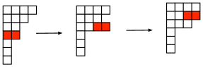
Figure 1: Example of an admissible move of type $a)$.

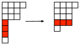
Figure 2: Example of an admissible move of type $b)$. The number of boxes of the new row is $3$: if it was 2, the move would not be admissible.

Remark 3.1.

If $\lambda=(1,1,...,1)$ there are no possible admissible moves.

Now we equip $\Lambda_{n}$ with the following partial order: $\lambda\in\Lambda_{n}$ is greater than $\mu\in\Lambda_{n}$ (we write $\lambda>\mu$) if $\lambda\neq\mu$ and the Young diagram of $\lambda$ can be obtained by the one of $\mu$ by a sequence of admissible moves (see Figure 3).

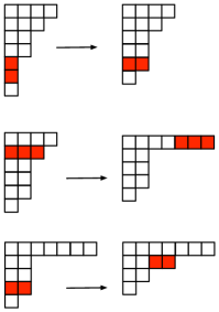
Figure 3: A sequence of three admissible moves, starting from the partition $\mu=(4,3,2,2,1,1,1)$. At the end we obtain $\lambda=(7,4,2,1)$, therefore $\lambda>\mu$.

In the sequel we will be interested in the subset $B\Lambda_{n}$ of $\Lambda_{n}$ ($n\geq 1$) made by $(n)$ and, if $n\geq 4$, by all the partitions with at least two numbers greater than or equal to 2, i.e. $\lambda\in B\Lambda_{n}$ iff $\lambda=(n)$ or $\lambda=(\lambda_{1},\lambda_{2},\ldots,\lambda_{k},...)$ with $k\geq 2$ and

$$\lambda_{1}\geq\lambda_{2}\geq\cdots\geq\lambda_{k}\geq 2$$

We will call building partitions the partitions in $B\Lambda_{n}$. The ordering of $\Lambda_{n}$ induces a poset structure on $B\Lambda_{n}$.

Remark 3.2.

Let $\gamma,\delta$ be two building partitions. If $\gamma\geq\delta$ one can find a subspace of the form $\gamma$ which contains a subspace of the form $\delta$.

Remark 3.3.

Let us denote by $\succeq$ the well known partial ordering on $\Lambda_{n}$ such that $\mu\succeq\gamma$ if and only if $\mu_{1}\geq\lambda_{1}$ and $\mu_{1}+\mu_{2}\geq\lambda_{1}+\lambda_{2}$ and so on. We observe that $\gamma\geq\lambda$ implies $\gamma\succeq\lambda$ but the reverse implication is not true. In fact the ordering $\succeq$ can be obtained as a result of a set of moves which includes the moves used to define $\geq$: the elementary steps consist in removing a box from a row of a Young diagram and adding it to a higher row. We notice that, for instance, $(5,2)\succeq(4,3)$ but one cannot find a subspace of the form $(4,3)$ inside a subspace of the form $(5,2)$.

Remark 3.4.

Given two partitions $\lambda,\gamma$ in the poset $(B\Lambda_{n},\geq)$, it is not true that there exists a minimum element $\mu\in B\Lambda_{n}$ such that $\mu\geq\lambda$ and $\mu\geq\gamma$. Let us consider for instance $\lambda=(8,4,4),\gamma=(7,5,3,1)$. The (not comparable) partitions $\theta=(12,4)$ and $\rho=(8,8)$ are the minimal partitions in $B\Lambda_{n}$ which are $\geq\lambda,\gamma$. Furthermore, it is not true that there exists a maximum element $\mu\in B\Lambda_{n}$ such that $\theta\geq\mu$ and $\rho\geq\mu$.

4 The $S_{n}$ invariant building sets of type $A_{n-1}$

We are going to to describe all the building sets associated to the root arrangement $A_{n-1}$ which are invariant with respect to the natural $S_{n}$ action (this is in the spirit of the construction of the compactifications of configuration spaces: the corresponding wonderful models will have a $S_{n}$ equivariant divisor at the boundary).

We start by defining a family of building sets, parametrized by building partitions.

Definition 4.1.

Let $\lambda$ be a building partition. We define ${\widetilde{\mathcal{G}}}_{\lambda}$ as the set made by all the subspaces of the form $\gamma\in\Lambda_{n}$ for every $\gamma\geq\lambda$. We define ${\mathcal{G}}_{\lambda}$ as ${\mathcal{F}}_{A_{n-1}}\cup{\widetilde{\mathcal{G}}}_{\lambda}$.

Remark 4.1.

We notice that, according to the definition, if $\lambda=(n)$ then ${\mathcal{G}}_{\lambda}$ is the building set of irreducibles ${\mathcal{F}}_{A_{n-1}}$. The only building set associated to the root system $A_{2}$ (i.e. when $n=3$) is ${\mathcal{G}}_{(3)}={\mathcal{F}}_{A_{2}}$. If $n=4$, there are two building sets: the minimal one ${\mathcal{G}}_{(4)}={\mathcal{F}}_{A_{3}}$ and the maximal one ${\mathcal{G}}_{(2,2)}$. If $n>4$, the maximal building set is ${\mathcal{G}}_{(2,2,1,1,1,...)}$.

It is immediate from the definition that:

Proposition 4.1.

Given two different building partitions $\mu$ and $\lambda$, the building set ${\mathcal{G}}_{\lambda}$ is included in ${\mathcal{G}}_{\mu}$ if and only if $\lambda>\mu$.

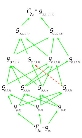
Figure 4: The Hasse diagram of the family of building sets of type ${\mathcal{G}}_{\lambda}$ in the case $A_{7}$ (green arrows represent inclusions). The red arrow shows a case where there is not inclusion.

The building sets of type ${\mathcal{G}}_{\lambda}$ ($\lambda\in B\Lambda_{n}$) are not the only $S_{n}$ invariant building sets which include ${\mathcal{F}}_{A_{n-1}}$. For instance, in the $A_{5}$ case, ${\mathcal{G}}_{(4,2)}\cup{\mathcal{G}}_{(3,3)}$ is an $S_{6}$ invariant building set, which does not belong to the family ${\mathcal{G}}_{\lambda}$. The following theorem describes all the $S_{n}$ invariant building sets.

Definition 4.2.

Given a set ${\mathcal{S}}=\{\lambda^{1},\lambda^{2},...,\lambda^{v}\}$ of pairwise not comparable elements in $B\Lambda_{n}$, we denote by ${\mathcal{G}}_{{\mathcal{S}}}$ the building set

$${\mathcal{G}}_{{\mathcal{S}}}={\mathcal{G}}_{\lambda^{1}}\cup{\mathcal{G}}_{\lambda^{2}}\cup...\cup{\mathcal{G}}_{\lambda^{v}}$$

We denote by ${\mathcal{T}}_{n}$ the set whose elements are the nonempty sets of pairwise not comparable elements in $B\Lambda_{n}$.

Theorem 4.1.

The map:

$${\mathcal{S}}=\{\lambda^{1},\lambda^{2},...,\lambda^{v}\}\rightarrow{\mathcal{G}}_{{\mathcal{S}}}$$

is a bijection between ${\mathcal{T}}_{n}$ and the set made by the $S_{n}$ invariant building sets which contain ${\mathcal{F}}_{A_{n-1}}$.

Proof.

Let us consider a $S_{n}$ invariant building set ${\mathcal{B}}$ which contains ${\mathcal{F}}_{A_{n-1}}$. If it is different from ${\mathcal{F}}_{A_{n-1}}$ we consider the subspaces in ${\mathcal{B}}-{\mathcal{F}}_{A_{n-1}}$: to each of these subspaces we associate the partition in $B\Lambda_{n}$ which describes its form and, among these partitions, we choose the minimal ones (with respet to $\geq$).

Let $A$ be a subspace in ${\mathcal{B}}-{\mathcal{F}}_{A_{n-1}}$ whose associated partition $\gamma=(\gamma_{1},\gamma_{2},\ldots,\gamma_{s})\in B\Lambda_{n}$ is minimal. Then, by $S_{n}$ invariance, ${\mathcal{B}}$ contains all the subspaces of this form. We will show that ${\mathcal{G}}_{\gamma}\subseteq{\mathcal{B}}$. For this it suffices to show that if $\mu\in B\Lambda_{n}$ can be obtained from $\gamma$ by an admissible move, than ${\mathcal{B}}$ contains all the subspaces of the form $\mu$. Let us consider moves of type $a)$: then $\mu=(\mu_{1},\mu_{2},\ldots,\mu_{i},...,\mu_{s-1})$ where the numbers $\mu_{l}$ coincide with the $\gamma_{h}$ except for $\mu_{i}=\gamma_{j}+\gamma_{t}$, where $\gamma_{j}>1$. Now we take two subspaces which are of the form $\gamma$ and therefore belong to ${\mathcal{B}}$:

$$C=\underset{\gamma_{1}}{\{\ldots\}}\underset{\gamma_{2}}{\{\ldots\}}...\underset{\gamma_{j}}{\{1,2,3,...,\gamma_{j}\}}\cdots\underset{\gamma_{t}}{\{\gamma_{j}+1,\gamma_{j}+2,...,\gamma_{j}+\gamma_{t}\}}\cdots\underset{\gamma_{s}}{\{\ldots\}}$$

$$D=\underset{\gamma_{1}}{\{\ldots\}}\underset{\gamma_{2}}{\{\ldots\}}...\underset{\gamma_{j}}{\{\gamma_{j}+1,2,3,...,\gamma_{j}\}}\cdots\underset{\gamma_{t}}{\{1,\gamma_{j}+2,...,\gamma_{j}+\gamma_{t}\}}\cdots\underset{\gamma_{s}}{\{\ldots\}}$$

The sum $C+D$ is the subspace

$$C+D=\underset{\gamma_{1}}{\{\ldots\}}\underset{\gamma_{2}}{\{\ldots\}}...\underset{\gamma_{j}+\gamma_{t}}{\{1,2,3,...,\gamma_{j},\gamma_{j}+1,\gamma_{j}+2,...,\gamma_{j}+\gamma_{t}\}}\cdots\underset{\gamma_{s}}{\{\ldots\}}$$

By definition of building set, $C+D$ must be the direct sum of the maximal subspaces in ${\mathcal{B}}$ contained in it. This is possible only if $C+D\in{\mathcal{B}}$. We have shown that ${\mathcal{B}}$ contains a subspace of the form $\mu$, and therefore it contains all such subspaces.

As for the moves of type $b)$, let $\gamma_{k}$ be the last part which is $>1$ of $\gamma\in B\Lambda_{n}$. As a particular case, we first show that if $\mu$ is obtained from $\gamma$ by deleting $\gamma_{k}$ parts equal to $1$ and adding a part equal to $\gamma_{k}$ then ${\mathcal{B}}$ contains a subspace of the form $\mu$. The argument is similar to the one above. For instance, if $\gamma=(4,3,1,1,1,1)$ and $\mu=(4,3,3,1)$, one then considers the two subspaces:

$$C=\{1,2,3,4\}\{5,6,7\}\{8\}\{9\}\{10\}\{11\}$$

$$D=\{1,2,3,4\}\{8,9,10\}\{5\}\{6\}\{7\}\{11\}$$

The sum $C+D$ is the subspace

$$C+D=\{1,2,3,4\}\{5,6,7\}\{8,9,10\}\{11\}$$

which must belong to ${\mathcal{B}}$ and has the form $\mu$. Combining the result in this particular case with the result for moves of the first type, it is now easy to prove that if $\mu\in B\Lambda_{n}$ can be obtained from $\gamma$ by any admissible move of the second type, than ${\mathcal{B}}$ contains all the subspaces of the form $\mu$.

Let $S=\{\gamma^{1},\gamma^{2},...,\gamma^{v}\}$ be the set of the (pairwise not comparable) minimal partitions associated to the subspaces in ${\mathcal{B}}-{\mathcal{F}}_{A_{n-1}}$. Repeating the argument described above we can prove that ${\mathcal{B}}$ contains ${\mathcal{G}}_{\gamma^{1}}\cup{\mathcal{G}}_{\gamma^{2}}\cup...\cup{\mathcal{G}}_{\gamma^{v}}$.

To show the reverse inclusion, let us consider $D\in{\mathcal{B}}-{\mathcal{F}}_{A_{n-1}}$. If $D$ is associated to a minimal partition, say $\gamma^{1}$, then $D\in{\mathcal{G}}_{\gamma^{1}}$ by definition. If the partition $\gamma$ associated to $D$ is not minimal, then for a certain $i$ we have $\gamma>\gamma^{i}$. By definition of ${\mathcal{G}}_{\gamma^{i}}$ we know that $D\in{\mathcal{G}}_{\gamma^{i}}$: this concludes the proof that ${\mathcal{B}}={\mathcal{G}}_{\gamma^{1}}\cup{\mathcal{G}}_{\gamma^{2}}\cup...\cup{\mathcal{G}}_{\gamma^{v}}$.

Now we must show that the above expression for ${\mathcal{B}}$ is unique, i.e., if ${\mathcal{B}}={\mathcal{G}}_{\lambda^{1}}\cup{\mathcal{G}}_{\lambda^{2}}\cup...\cup{\mathcal{G}}_{\lambda^{v}}$ and ${\mathcal{B}}={\mathcal{G}}_{\theta^{1}}\cup{\mathcal{G}}_{\theta^{2}}\cup...\cup{\mathcal{G}}_{\theta^{r}}$ then $r=v$ and, up to reordering, $\theta^{i}=\lambda^{i}$ $\forall i$. Let us suppose that ${\mathcal{B}}\neq{\mathcal{F}}_{A_{n-1}}$ (otherwise the statement is trivial).

First we observe that if $\lambda^{1}$ is not $\geq$ of one of the partitions $\theta^{1},\theta^{2},...,\theta^{r}$, then in ${\mathcal{G}}_{\theta^{1}}\cup{\mathcal{G}}_{\theta^{2}}\cup...\cup{\mathcal{G}}_{\theta^{r}}$ there are not elements of the form $\lambda^{1}$. This is a contradiction. Therefore we must have, say, $\lambda^{1}\geq\theta^{1}$. The same argument shows that there exists $i$ such that $\theta^{1}\geq\lambda^{i}$. This implies $\lambda^{1}\geq\lambda^{i}$, and since the elements $\lambda^{1},\lambda^{2},...,\lambda^{v}$ are pairwise not comparable, we must have $i=1$ and $\lambda^{1}\geq\theta^{1}\geq\lambda^{1}$, that is to say, $\lambda^{1}=\theta^{1}$. The claim follows by induction.

∎

5 The Poincaré polynomial for the maximal model (case $A_{n-1}$)

In this section we provide a formula for the Poincaré polynomial of the maximal model $Y_{{\mathcal{G}}_{(2,2,1,1,....)}}=Y_{max,n}$:

$$P(Y_{max,n})(q)=\sum_{i}dim\ H^{2i}(Y_{max,n},{\mathbb{Q}})q^{i}$$

We use a combinatorial strategy, different from the one in [15], which in the next sections will be generalized in many ways (i.e. it will be applied to different models and to different root arrangements).

Let $G$ be a minimal (with respect to inclusion) element in a building set ${\mathcal{G}}$. Let ${\mathcal{G}}^{\prime}={\mathcal{G}}-\{G\}$, and let ${\overline{\mathcal{G}}}$ be the family in ${\displaystyle\left({\mathbb{C}}^{n}\right)^{\ast}/G}$ given by the elements $\{(A+G)/G\>:\>A\in{\mathcal{G}}^{\prime}\}$. In [4] and [13] it is shown that ${\mathcal{G}}^{\prime}$ and ${\overline{\mathcal{G}}}$ are building and that $Y_{{\mathcal{G}}}$ can be obtained by blowing up $Y_{{\mathcal{G}}^{\prime}}$ along a subvariety isomorphic to $Y_{{\overline{\mathcal{G}}}}$.

This implies that, denoting by $p$ the blowing up map ${\displaystyle p\>:\>Y_{{\mathcal{G}}}\mapsto Y_{{\mathcal{G}}^{\prime}}}$, we have

$$H^{\ast}(Y_{{\mathcal{G}}},{\mathbb{Z}})\cong p^{\ast}H^{\ast}(Y_{{\mathcal{G}}^{\prime}},{\mathbb{Z}})\oplus\left(H^{\ast}(E,{\mathbb{Z}})/p^{\ast}H^{\ast}(Y_{{\overline{\mathcal{G}}}},{\mathbb{Z}})\right)$$

The exceptional divisor $E$ is isomorphic to the projectivization of the normal bundle of $Y_{{\overline{\mathcal{G}}}}$ in $Y_{{\mathcal{G}}^{\prime}}$. Then $H^{\ast}(E,{\mathbb{Z}})$ is generated, as $p^{\ast}H^{\ast}(Y_{{\overline{\mathcal{G}}}},{\mathbb{Z}})$-algebra, by the Chern class $\zeta=c_{1}(T)$ of the tautological line bundle $T\mapsto E$. Furthermore the class $\zeta$ has in $H^{\ast}(E,{\mathbb{Z}})$ the unique relation provided by the Chern polynomial of the normal bundle $N_{Y_{{\overline{\mathcal{G}}}}/Y_{{\mathcal{G}}^{\prime}}}$. This proves the following proposition where we denote by $P(Y)(q)$ ($q$ has degree 2) the Poincarè polynomial of a model $Y$:

Proposition 5.1.

Let $G$ be a minimal (with respect to inclusion) element in a building set ${\mathcal{G}}$. Then:

$$P(Y_{{\mathcal{G}}})(q)=P(Y_{{\mathcal{G}}^{\prime}})(q)+\frac{q^{dim\,G}-q}{q-1}P(Y_{{\overline{\mathcal{G}}}})(q)$$

Theorem 5.1.

For $n\geq 2$, we have the following inductive formula for the Poincaré polynomial of the maximal model $Y_{{\mathcal{G}}_{(2,2,1,1,....)}}=Y_{max,n}$:

$$P(Y_{max,n})(q)=1+\sum_{\begin{array}[]{c}\lambda\in\Lambda_{n}\\ \lambda\neq(1,1,1,...,1)\end{array}}\frac{q^{n-l(\lambda)}-q}{q-1}t_{\lambda}P(Y_{max,l(\lambda)})(q)$$

where $l(\lambda)$ is the lenght of the partition $\lambda$ (the number of parts) and $t_{\lambda}$ is the number of subspaces whose form is $\lambda$.

Proof.

We obtain this formula by applying Proposition 5.1 several times. We start by choosing a minimal subspace in the building set ${\mathcal{G}}_{(2,2,1,1,....)}$, then a minimal subspace in the building set ${\mathcal{G}}_{(2,2,1,1,....)}^{\prime}$ and so on.

The key observation is that the ‘quotient’ building sets which are produced by this process are all isomorphic to maximal building sets. More precisely, let us suppose that, at a certain step, we have the building set ${\mathcal{G}}_{(2,2,1,1,....)}^{\prime\prime}={\mathcal{G}}_{(2,2,1,1,....)}-\{\hbox{some subspaces}\}$. The dimension of the deleted subspaces can be bounded, since at every step we have to remove a minimal subspace, so at first we can remove the subspaces of dimension 2, then the subspaces of dimension 3, and so on. Let us therefore suppose that in ${\mathcal{G}}_{(2,2,1,1,....)}^{\prime\prime}$ the deleted subspaces are of dimension $\leq j$. Now we remove a minimal subspace $A$ from ${\mathcal{G}}_{(2,2,1,1,....)}^{\prime\prime}$: if there still are subspaces of dimension $j$ in ${\mathcal{G}}_{(2,2,1,1,....)}^{\prime\prime}$ then $A$ has dimension $j$, otherwise $A$ has dimension $j+1$. Let $A$ have the form $\lambda$. Now let us consider $\overline{{\mathcal{G}}^{\prime\prime}}$: it is isomorphic to a building set associated to the arrangement $A_{l(\lambda)-1}$. In fact we can think of the quotient space as the space where some groups of variables are equal: there are only $l(\lambda)$ ‘free variables’. From this point of view, it is easy to check that $\overline{{\mathcal{G}}^{\prime\prime}}$ is the maximal building set of type $A_{l(\lambda)-1}$: every subspace in this maximal building set can be obtained as a quotient $B+A/A$, where we can choose $B\in{\mathcal{G}}_{(2,2,1,1,....)}$ with $dim\ B>dim\ A$, so $B\in{\mathcal{G}}_{(2,2,1,1,....)}^{\prime\prime}$. ∎

Remark 5.1.

We put $P(Y_{max,1})(q)=1$ as a base for the induction. Then we observe that $P(Y_{max,2})(q)=1$ and $P(Y_{max,3})(q)=q+1$.

From this inductive formula we can write $P(Y_{max,n})(q)$ as an explicit sum of polynomials whose coefficients are expressed in terms of the Stirling numbers of the second kind.

Definition 5.1.

Given two positive integers $n>j$, let us denote by $f_{n,j}(q)$ the polynomial $S(n,j)\frac{q^{n-j}-q}{q-1}\;$, where $S(n,j)=\frac{Surg(n,j)}{j!}$ is the Stirling number of the second kind.

Theorem 5.2.

For $n\geq 3$, we have:

$$P(Y_{max,n})(q)=1+\sum_{\begin{array}[]{c}1\leq k\leq\lfloor\frac{n-1}{2}\rfloor\\ (j_{1},j_{2},...,j_{k})\in J_{k}(n-2)\end{array}}f_{j_{2},j_{1}}(q)f_{j_{3},j_{2}}(q)\cdots f_{j_{k},j_{k-1}}(q)f_{n,j_{k}}(q)$$

where $J_{k}(n-2)$ is the set of all the lists $(j_{1},j_{2},...,j_{k})$ of integers such that $1\leq j_{1}<j_{2}<\cdots<j_{k}\leq n-2$ and, for every $i=1,2,...,k$, $j_{i}-j_{i-1}\geq 2$.

Proof.

The proof is by induction on $n$.

One first observes that, in the sum which appears in the formula of Theorem 5.1, we can regroup all the partitions with the same length $j$, with $j=1,...,n-2$:

$$P(Y_{max,n})(q)=1+\sum_{j=1,....,n-2}\frac{q^{n-j}-q}{q-1}\;S(n,j)P(Y_{max,j})(q)$$

The conclusion then follows by induction. ∎

Remark 5.2.

We notice that we can use our formula for the Poincaré polynomials of the maximal models to obtain formulas for $P(Y_{{\mathcal{G}}_{(2,2,1,1,....)}^{\prime\prime}})(q)$, where ${\mathcal{G}}_{(2,2,1,1,....)}^{\prime\prime}$ is any one of the building sets obtained as a result of the above described algorithm, which starts from ${\mathcal{G}}_{(2,2,1,1,....)}$ and deletes at each step a minimal subspace. In fact, at each step of the algorithm we have a relation like the following one:

$$P(Y_{max,n})(q)=P(Y_{{\mathcal{G}}_{(2,2,1,1,....)}^{\prime\prime}})(q)+\hbox{sums of polynomials}\ \frac{q^{n-j}-q}{q-1}P(Y_{max,j})(q)$$

In principle it is possible to use arguments similar to the one used in the proof of Theorem 5.1 to find formulas for the Poincaré polynomials of the models $Y_{{\mathcal{G}}_{\lambda}}$ ($\lambda\in B\Lambda_{n}$), but when we quotient by a subspace it is not always true that the quotient building set is one of the invariant ones described in the preceding sections, so the computation may need further steps and may become more complicated.

6 Regular building sets

The following building sets appear as natural objects in our picture, since they are obtained as unions of the building sets ${\mathcal{G}}_{\lambda}$ which lie on a same row of the diagram of $B\Lambda_{n}$ (see Figure 4).

Definition 6.1.

For every $n\geq 3$ and $1\leq s\leq n-2$ we denote by ${\mathcal{G}}_{s}(A_{n-1})$ the $S_{n}$ invariant building set which contains ${\mathcal{F}}_{A_{n-1}}$ and also all the subspaces of the maximal building set which have dimension $\geq n-s$. We will call ${\mathcal{G}}_{s}(A_{n-1})$ the regular building set of degree $s$.

We notice that, for $n\geq 3$, ${\mathcal{G}}_{1}(A_{n-1})={\mathcal{F}}_{A_{n-1}}={\mathcal{G}}_{(n)}$ and, for $n\geq 4$, ${\mathcal{G}}_{n-2}(A_{n-1})$ is equal to the maximal building set ${\mathcal{G}}_{(2,2,1,...,1)}$. Therefore, for every $n\geq 3$ we have pointed out $n-2$ distinct regular building sets which include the irreducibles:

$${\mathcal{G}}_{1}(A_{n-1})\subset{\mathcal{G}}_{2}(A_{n-1})\subset\cdots\subset{\mathcal{G}}_{n-2}(A_{n-1}).$$

The following definition points out the property needed to apply the argument of the proof of Theorem 5.1 to more general building sets.

Definition 6.2.

Let us consider, for every $n\geq 1$, a building set ${\mathcal{G}}(n)$ (associated to a subspace arrangement in ${\mathbb{C}}^{n}$). We will call the family $\{{\mathcal{G}}(n)\}$ inductive if, when we take any subspace $G\in{\mathcal{G}}(n)$ of dimension $j$ (with $n-1\geq j>2$), the building set ${\overline{\mathcal{G}}(n)}=\{(A+G)/G\>:\>A\in{\mathcal{G}}^{\prime\prime}\}$ is (isomorphic to) ${\mathcal{G}}(n-j)$, for every ${\mathcal{G}}^{\prime\prime}$ obtained from ${\mathcal{G}}$ by removing $G$, all the subspaces of dimension $<j$ and any collection of subspaces of dimension $j$.

A first remark is that the family of maximal building sets is inductive.

We observe that ${\mathcal{G}}_{n-3}(A_{n-1})$ is an inductive family, while ${\mathcal{G}}_{n-4}(A_{n-1})$ is inductive “up to subspaces of dimension 1”, that is to say, the quotient building sets may differ from the expected ones, but only in the subspaces of dimension 1. For $s<n-4$ the family ${\mathcal{G}}_{s}(A_{n-1})$ is not inductive, so the argument of the proof of Theorem 5.1 cannot be applied. Anyway we will manage to compute the Poincaré polynomials of the associated models. For this it is useful to introduce some different families of building sets, which are inductive:

Definition 6.3.

For every $n\geq 3$ and $1\leq s\leq n-1$ we denote by ${\widetilde{\mathcal{G}}}_{s}(A_{n-1})$ the ($S_{n}$ invariant) building set which contains all the subspaces of the maximal building set which have dimension $\geq n-s$.

Remark 6.1.

We notice that ${\widetilde{\mathcal{G}}}_{n-1}(A_{n-1})={\mathcal{G}}_{n-2}(A_{n-1})$ and that all the other building sets ${\widetilde{\mathcal{G}}}_{s}(A_{n-1})$ (when $1\leq s\leq n-2$) do not include hyperplanes. All the families ${\widetilde{\mathcal{G}}}_{s}(A_{n-1})$ are inductive.

For convenience of notation, for every $n\geq 2$ and $s\geq n-1$ we put ${\mathcal{G}}_{s}(A_{n-1})$ and ${\widetilde{\mathcal{G}}}_{s+1}(A_{n-1})$ to be equal to the maximal building set. Let us denote by $f_{n,j}(q)$, as in Section 5, the polynomial $S(n,j)\frac{q^{n-j}-q}{q-1}\;$ (where $S(n,j)$ are the Stirling numbers of the second kind).

Theorem 6.1.

For every $n\geq 3$ and $1\leq s\leq n-2$ we have the following formula for the Poincaré polynomial of the models $Y_{{\widetilde{\mathcal{G}}}_{s}(A_{n-1})}$:

$$P(Y_{{\widetilde{\mathcal{G}}}_{s}(A_{n-1})})(q)=1+\sum_{\begin{array}[]{c}1\leq k\leq\lfloor\frac{s+1}{2}\rfloor\\ (j_{1},j_{2},...,j_{k})\in J_{k}(s)\end{array}}f_{j_{2},j_{1}}(q)f_{j_{3},j_{2}}(q)\cdots f_{j_{k},j_{k-1}}(q)f_{n,j_{k}}(q)$$

Proof.

One repeats the steps of the proofs of Theorems 5.1 and 5.2, paying attention to the fact that the length of the partitions which appear is $\leq s$. ∎

Remark 6.2.

Since ${\widetilde{\mathcal{G}}}_{n-2}(A_{n-1})$ and ${\mathcal{G}}_{n-2}(A_{n-1})$ differ only in the subspaces of dimension 1, this formula includes as a particular case ($s=n-2$) the formula for the maximal models (see Theorem 5.2).

Now we are ready to describe formulas for the Poincaré polynomials of the models $Y_{{\mathcal{G}}_{s}(A_{n-1})}$: these turn out to be interpolations between the well known formula for minimal models and the formula for maximal models of Theorem 5.2. In these interpolations the polynomials $P(Y_{{\widetilde{\mathcal{G}}}_{s}(A_{n-1})})(q)$ play a role.

In [26] the Poincaré series $\Phi(q,t)=t+\sum_{n\geq 2,i}dim\ H^{2i}(Y_{{\mathcal{G}}_{1}(A_{n-1})},{\mathbb{Q}})q^{i}\frac{t^{n}}{n!}$ for the minimal models has been computed in the following way. First one computes, via a recursive relation, the series $\lambda(q,t)$ which counts the contribution of basis monomials whose associated nested set is represented by a tree (included the degenerate tree given by a single leaf, which gives contribution $t$):

$$\lambda(q,t)^{(1)}=1+\frac{\lambda(q,t)^{(1)}}{q-1}\left[e^{q\lambda(q,t)}-qe^{\lambda(q,t)}+q-1\right]$$

(here the superscript ⁽¹⁾ means the first derivative with respect to $t$).

Then one obtains $\Phi(q,t)$ as $e^{\lambda(q,t)}-1$.

Now we need a modification $\Phi(q,t,y)$ of $\Phi(q,t)$, where the powers of the variable $y$ take into account the number of the maximal subspaces in the nested sets associated to basis elements:

$$\Phi(q,t,y)=e^{y\lambda(q,t)}-1$$

Theorem 6.2.

For every $n\geq 3$ and $1\leq s\leq n-2$ we have the following formula for the Poincaré polynomial of the models $Y_{{\mathcal{G}}_{s}(A_{n-1})}$:

$$\frac{t^{n}}{n!}P(Y_{{\mathcal{G}}_{s}(A_{n-1})})(q)=\frac{t^{n}}{n!}P(Y_{{\widetilde{G}}_{s}(A_{n-1})})(q)+$$

$$+\sum_{\begin{array}[]{c}s<j\leq n-2\end{array}}\Phi_{|{\small\begin{array}[]{c}deg\ y=j\\ deg\ t=n\end{array}}}(q,t,1)P(Y_{{\widetilde{\mathcal{G}}}_{s}(A_{j-1})})(q)$$

Proof.

Our first step consists in describing the ${\mathcal{G}}_{s}(A_{n-1})$-nested sets, since they are the supports of the monomials of the Yuzvinski bases (see Section 2.2). One observes that, if $S$ is a ${\mathcal{G}}_{s}(A_{n-1})$-nested set, then $S$ can be partitioned into two subsets:
a) the (possibly empty) subset $S_{1}$ made by the subspaces which belong to ${\widetilde{\mathcal{G}}}_{s}(A_{n-1})$. If $S_{1}$ is not empty, it contains a minimal element $A$ (with respect to inclusion). Then the elements of $S_{1}$ are totally orderd by inclusion ($A$ is the minimal one).
b) the (possibly empty) subset $S_{2}$ made by the subspaces which belong to ${\mathcal{F}}_{A_{n-1}}-{\widetilde{\mathcal{G}}}_{s}(A_{n-1})$. They satisfy the following properties: they form a ${\mathcal{F}}_{A_{n-1}}$-nested set; their sum $B$ doesn’t belong to ${\widetilde{\mathcal{G}}}_{s}(A_{n-1})$ and, if $S_{1}$ is not empty and $A$ is the minimal subspace in $S_{1}$, $B$ is strictly included into $A$.

Therefore, every monomial $m$ in the basis is the product of a monomial $m_{S_{1}}$ with support in $S_{1}$ and a monomial $m_{S_{2}}$ with support in $S_{2}$. We notice that $m_{S_{2}}$ also belongs to the cohomology basis of $Y_{{\mathcal{F}}_{A_{n-1}}}$.

Let us denote by $A_{1},A_{2},...,A_{t}$ the maximal elements in $S_{2}$. We can represent them by subsets of $\{1,2,...,n\}$ as usual; considering the cardinalities of these subsets, and eventually adding some parts equal to 1, we can associate to $A_{1},A_{2},...,A_{t}$ a partition $\lambda\in\Lambda_{n}$.

One can then compute Poincaré polynomials by regrouping all the basis monomials such that the maximal elements in $S_{2}$ give a partition of length $j$, with the two following restrictions on $j$: $j\leq n-2$ (all the subspaces $A_{1},A_{2},...,A_{t}$ have dimension $\geq 2$ otherwise they are not in the support of a basis element) and $j>s$ (otherwise $A_{1}+A_{2}+\cdots+A_{t}$ belongs to ${\mathcal{G}}_{s}(A_{n-1})$).

The contribution of all the “$m_{S_{2}}$ factors” such that the maximal elements in $S_{2}$ give a partition of length $j$ is provided (up to multiplication by $\frac{t^{n}}{n!}$) by:

$$\Phi_{|{\small\begin{array}[]{c}deg\ y=j\\ deg\ t=n\end{array}}}(q,t,1)$$

Now we observe that, by our description of nested sets, once such a factor $m_{S_{2}}$ is fixed, all the factors of type $m_{S_{1}}$ are in bijective correspondence with the monomials of the cohomology basis of $Y_{{\widetilde{\mathcal{G}}}_{s}(A_{j-1})}$. The following example illustrates this correspondence: let $n=12$ and let $\{1,2,3\}$ and $\{4,5,6,7\}$ be the maximal subspaces in $S_{2}$. Then every subspace in $S_{1}$ contains $\{1,2,3\}$ and $\{4,5,6,7\}$, therefore we can represent it as a partition of $\{1,2,...,12\}$ where 1,2,3 belong to the same part, and 4,5,6,7 belong to the same part. Now, “collapsing” 1,2,3 to a new symbol $\overline{1}$ and 4,5,6,7 to $\overline{4}$, we are representing every subspace in $S_{1}$ by a partition of $\{\overline{1},\overline{4},8,9,10,11,12\}$, or renumbering the elements, by a partition of $\{1,2,3,4,5,6,7\}$. In this way we associate to the monomial $m_{S_{1}}$ a monomial in the cohomology basis of $Y_{{\widetilde{\mathcal{G}}}_{s}(A_{6})}$ (in this correspondence the exponents do not change, according to the definition of admissible monomials in Section 2.2).

∎

Example 6.1.

Here there are some examples:

$$P(Y_{{\mathcal{G}}_{1}(A_{4})})(q)=q^{3}+16q^{2}+16q+1$$

$$P(Y_{{\mathcal{G}}_{2}(A_{4})})(q)=q^{3}+26q^{2}+26q+1$$

$$P(Y_{{\mathcal{G}}_{3}(A_{4})})(q)=q^{3}+41q^{2}+41q+1$$

$$P(Y_{{\mathcal{G}}_{1}(A_{5})})(q)=q^{4}+42q^{3}+127q^{2}+42q+1$$

$$P(Y_{{\mathcal{G}}_{2}(A_{5})})(q)=q^{4}+67q^{3}+222q^{2}+67q+1$$

$$P(Y_{{\mathcal{G}}_{3}(A_{5})})(q)=q^{4}+142q^{3}+372q^{2}+142q+1$$

$$P(Y_{{\mathcal{G}}_{4}(A_{5})})(q)=q^{4}+187q^{3}+732q^{2}+187q+1$$

$$P(Y_{{\mathcal{G}}_{5}(A_{6})})(q)=q^{5}+855q^{4}+9556q^{3}+9556q^{2}+855q+1$$

Remark 6.3 (There is not an extended action on non minimal models).

As it is well known, the minimal model of type $A_{n-1}$ has a natural ‘extended’ $S_{n+1}$ action, which comes from the moduli interpretation (see for instance [4], [13], [14]). This is not true for the other $S_{n}$ invariant models, as one can see from the geometrical point of view since the $S_{n}$ action induced on the irreducible divisors in the boundary does not extend to a $S_{n+1}$ action.

From the algebraic point of view, for instance, a comparison between the character $\chi^{2}_{4}$ of the $S_{4}$ action on $Y_{{\mathcal{G}}_{2}(A_{3})}$ and the character $\chi^{1}_{4}$ of the $S_{4}$ action on $Y_{{\mathcal{G}}_{1}(A_{3})}$ shows that on the cohomology of the maximal model there is not an extended action compatible with the extended action on the cohomology of the minimal model. In fact $\chi^{2}_{4}-\chi^{1}_{4}=(s_{(4)}+s_{(2,2)})q$ and there is not a representation of $S_{5}$ which, once restricted, decomposes as $s_{(4)}+s_{(2,2)}$.

7 Case $B_{n}$ ( and $C_{n}$), classification of all the invariant building sets

Let us consider the root arrangement of type $B_{n}$ in ${\mathbb{C}}^{n}$ and let $W(B_{n})$ be its Weyl group (the case $C_{n}$ leads to the same arrangement). The subspaces in the building set of irreducibles ${\mathcal{F}}_{B_{n}}$ are of two types, strong subspaces and weak subspaces. A subspace of $({\mathbb{C}}^{n})^{*}$ is strong if its annihilator can be described by the equation $x_{i_{1}}=\cdots=x_{i_{k}}=0$. Then strong subspaces can be put in bijective correspondence with the subsets of $\{1,\cdots,n\}$ of cardinality greater than or equal to $1$ (we will call such subsets strong when they represent a strong subspace). A subspace in ${\mathcal{F}}_{B_{n}}$ is weak if its annihilator can be described by $\{x_{i_{1}}=\cdots=x_{i_{r}}=-x_{j_{1}}=\cdots=-x_{j_{s}}\}$ ($r+s\geq 2$); therefore weak elements are in bijective correspondence with the subsets of $\{1,\cdots,n\}$ of cardinality greater than or equal to $2$ (such subsets will be called weak) equipped with a partition (possibly trivial) into two parts.

Therefore, the subspaces in the maximal building set ${\mathcal{C}}_{B_{n}}$ can put in bijective correspondence with the partitions of $\{1,\cdots,n\}$ such that each part is labelled "weak" or "strong" and the following extra conditions are satisfied: at most one part is strong, and if there is not a strong part, then at least one of the weak parts has more than 1 element.

We want to classify all the $W(B_{n})$ invariant building sets which include ${\mathcal{F}}_{B_{n}}$. The combinatorial description of the subspaces in the maximal building set suggests us to introduce the notion of partition with a singular part:

Definition 7.1.

We denote by $S\Lambda_{n}$ the set of singular partitions: its elements are the couples $(r,\lambda)$ with $r$ integer, $0\leq r\leq n$ and $\lambda\in\Lambda_{n-r}$.

If a subspace $A$ in ${\mathcal{C}}_{B_{n}}$ is represented by a partition of $\{1,\cdots,n\}$, which has a strong part of cardinality $r$ ($r$ may be 0) and weak parts whose cardinalities give the partition $\lambda\in\Lambda_{n-r}$, we will say that $A$ has the form $(r,\lambda)$.

The element $(r,\lambda)\in S\Lambda_{n}$ can be represented by a diagram whose higher row has $r$ coloured boxes (see Figure 5).

Figure 5: The coloured diagram representing the singular (building) partition $(2,(4,3,1,1,1))$.

We consider the following three types of admissible moves on $S\Lambda_{n}$:
a) remove an entire not coloured row and add all its boxes to a not coloured row which has at least two boxes or to the coloured row (if it exists; if we are adding boxes to the coloured row, then the boxes will be coloured). At the end, if necessary, the not coloured rows will be rearranged in order to obtain a valid diagram;
b) remove $k\geq 2$ not coloured rows made by a single box and form a row made by $k$ boxes, if $k$ is greater than or equal to the number of boxes of the smallest not coloured row with more than one box; then, if necessary, rearrange the rows in order to obtain a valid coloured diagram;
c) if the diagram is made by a single row, we can colour it.

As in the $A_{n}$ case, we introduce a partial ordering in $S\Lambda_{n}$:

$$(s,\gamma)\geq(r,\lambda)$$

if and only if $(s,\gamma)$ can be obtained by $(r,\lambda)$ by a sequence of admissible moves.

Definition 7.2.

A singular building partition (of type $B_{n}$, $n\geq 2$) is a couple $(r,\lambda)\in S\Lambda_{n}$ which satisfies the further conditions that $\lambda\neq(1,1,1,...)$ and, if $r=0$, then $\lambda\in B\Lambda_{n}-\{(n)\}$. We will denote by $SB\Lambda_{n}$ the poset of all singular building partitions, with the ordering induced by $\geq$.

Definition 7.3.

Let us consider $(r,\lambda)\in SB\Lambda_{n}$. We define the set $B{\mathcal{G}}_{(r,\lambda)}$ as the union of ${\mathcal{F}}_{B_{n}}$ with the set made by all the subspaces of the form $(s,\gamma)\in SB\Lambda_{n}$, with $(s,\gamma)\geq(r,\lambda)$.

We notice that, according to the definition, the building set of irreducibles is denoted by $B{\mathcal{G}}_{(n,(0))}$. If $n=3$, there are two $W(B_{n})$ invariant building sets which contain the irreducibles: the minimal one $B{\mathcal{G}}_{(3,(0))}$ and the maximal one $B{\mathcal{G}}_{(1,(2))}$. If $n>3$, the building sets $B{\mathcal{G}}_{(s,\lambda)}$ ($(s,\lambda)$ in $SB\Lambda_{n}$) are all distinct and the maximal building set is described as $B{\mathcal{G}}_{(0,(2,2,1,1,1,...))}\cup B{\mathcal{G}}_{(1,(2,1,1,1,1,...))}$.

Proposition 7.1.

Given $n\geq 3$ and two different singular building partitions $(r,\mu)$ and $(s,\lambda)$ in $SB\Lambda_{n}$, the building set $B{\mathcal{G}}_{(s,\lambda)}$ is included into $B{\mathcal{G}}_{(r,\mu)}$ if and only if $(s,\lambda)>(r,\mu)$.

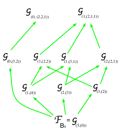
Figure 6: The Hasse diagram of the family of building sets of type ${\mathcal{G}}_{(r,\mu)}$ (with $(r,\mu)$ in $SB\Lambda_{n}$) in the case $B_{5}$.

Definition 7.4.

Given a set ${\mathcal{S}}=\{(r_{1},\lambda^{1}),(r_{2},\lambda^{2}),...,(r_{v},\lambda^{v})\}$ of pairwise not comparable elements in $SB\Lambda_{n}$, we denote by ${\mathcal{G}}_{{\mathcal{S}}}$ the building set

$${\mathcal{G}}_{{\mathcal{S}}}={\mathcal{G}}_{(r_{1},\lambda^{1})}\cup{\mathcal{G}}_{(r_{2},\lambda^{2})}\cup...\cup{\mathcal{G}}_{(r_{v},\lambda^{v})}$$

and by $B{\mathcal{T}}_{n}$ the set whose elements are the nonempty sets of pairwise not comparable elements in $SB\Lambda_{n}$.

We have the following classification theorem (we omit the proof, since it is similar to the $A_{n}$ case, Theorem 4.1).

Theorem 7.1.

The map:

$${\mathcal{S}}=\{(r_{1},\lambda^{1}),(r_{2},\lambda^{2}),...,(r_{v},\lambda^{v})\}\rightarrow{\mathcal{G}}_{{\mathcal{S}}}$$

is a bijection between $B{\mathcal{T}}_{n}$ and the set of the $W(B_{n})$ invariant building sets which contain the irreducibles.

8 Regular building sets in case $B_{n}$.

As in the $A_{n}$ case, we focus on the regular $W(B_{n})$ invariant building sets, obtained as the union of all the building sets of type ${\mathcal{G}}_{(r,\mu)}$ (with $(r,\mu)$ in $SB\Lambda_{n}$) which lie on a same row of the Hasse diagram (see Figure 6).

Definition 8.1.

For every $n\geq 2$ and $0\leq s\leq n-2$ we denote by ${\mathcal{G}}_{s}(B_{n})$ the ($W(B_{n})$ invariant) building set which contains the irreducibles and also all the subspaces of the maximal building set which have dimension $\geq n-s$. We will call ${\mathcal{G}}_{s}(B_{n})$ the regular building set of type $B_{n}$ and of degree $s$.

For every $n\geq 2$ and $s\geq n-1$ we put ${\mathcal{G}}_{s}(B_{n})$ to be equal to the maximal building set. We notice that, for $n\geq 3$, ${\mathcal{G}}_{0}(B_{n})$ is the building set of irreducibles (denoted by $B{\mathcal{G}}_{(n,(0))}$ in Section 7) and, for $n\geq 4$, ${\mathcal{G}}_{n-2}(B_{n})$ is equal to the maximal building set $B{\mathcal{G}}_{(0,(2,2,1,1,1,...))}\cup B{\mathcal{G}}_{(1,(2,1,1,1,1,...))}$.

As in the $A_{n}$ case, we will define families of subspace arrangements which are obtained by removing some of the irreducible subspaces from ${\mathcal{G}}_{s}(B_{n})$.

Definition 8.2.

For every $n\geq 2$ and $0\leq s\leq n-1$ we denote by ${\widetilde{\mathcal{G}}}_{s}(B_{n})$ the ($W(B_{n})$ invariant) building set which contains all the subspaces of the maximal building set which have dimension $\geq n-s$. Moreover, for every $n\geq 2$ and $s>n-1$ we put ${\widetilde{\mathcal{G}}}_{s}(B_{n})$ to be equal to the maximal building set.

We remark that ${\widetilde{\mathcal{G}}}_{n-1}(B_{n})={\mathcal{G}}_{n-2}(B_{n})$ is the maximal building set and that, for every fixed $s\geq 0$, the family ${\widetilde{\mathcal{G}}}_{s}(B_{n})$ is inductive.

Given two positive integers $n>j$, let us denote by $h_{n,j}(q)$ the polynomial

$$h_{n,j}(q)=\left(\sum_{k=1}^{n+1-(j-1)}\binom{n}{k-1}S(n+1-k,j-1)2^{n+1-(j-1)-k}\right)\frac{q^{n+1-j}-q}{q-1}$$

Theorem 8.1.

For every $n\geq 2$ and $0\leq s\leq n-2$ we have

$$P(Y_{{\widetilde{\mathcal{G}}}_{s}(B_{n})})(q)=1+\sum_{\begin{array}[]{c}1\leq k\leq\lfloor\frac{s+2}{2}\rfloor\\ (j_{1},j_{2},...,j_{k})\in J_{k}(s+1)\end{array}}h_{j_{2},j_{1}}(q)h_{j_{3},j_{2}}(q)\cdots h_{j_{k},j_{k-1}}(q)h_{n,j_{k}}(q)$$

where $J_{k}(s+1)$ is the set of all the lists $(j_{1},j_{2},...,j_{k})$ of integers such that $1\leq j_{1}<j_{2}<\cdots<j_{k}\leq s+1$ and, for every $i=1,2,...,k$, $j_{i}-j_{i-1}\geq 2$.

Proof.

We can compute the Poincaré polynomials using the strategy described in Section 5, i.e. by removing at each step a minimal element and considering the quotient. Since the family of building sets ${\widetilde{\mathcal{G}}}_{s}(B_{n})$ is inductive, every quotient is again a building set of type ${\widetilde{\mathcal{G}}}_{s}(B_{j})$. We then have the following inductive formula:

$$P(Y_{{\widetilde{\mathcal{G}}}_{s}(B_{n})})(q)=1+\sum_{\begin{array}[]{c}j=n-s+1,....,n\end{array}}\frac{q^{j-1}-q}{q-1}\binom{n}{j}2^{j-1}P(Y_{{\widetilde{\mathcal{G}}}_{s}(B_{n-j+1})})(q)+$$

$$+\sum_{\begin{array}[]{c}j=n-s,....,n-1\end{array}}\frac{q^{j}-q}{q-1}\binom{n}{j}P(Y_{{\widetilde{\mathcal{G}}}_{s}(B_{n-j})})(q)+$$

$$+\sum_{{\begin{array}[]{c}(r,\lambda)\in SB\Lambda_{n}\\ l(\lambda)\leq s\end{array}}}\frac{q^{n-l(\lambda)}-q}{q-1}\binom{n}{r}2^{n-r-l(\lambda)}t_{\lambda}P(Y_{{\widetilde{\mathcal{G}}}_{s}(B_{l(\lambda)})})(q)$$

The first (res. second) addendum describes the quotients by weak (resp. strong) subspaces in ${\mathcal{F}}_{B_{n}}\cap{\widetilde{\mathcal{G}}}_{s}(B_{n})$. The third addendum describes the quotients by subspaces in ${\widetilde{\mathcal{G}}}_{s}(B_{n})$ whose form $(r,\lambda)$ belongs to $SB\Lambda_{n}$. For every $j=1,...,s+1$ we can regroup all the subspaces which have dimension $n+1-j$, which are

$$\sum_{k=1}^{n+1-(j-1)}\binom{n}{k-1}S(n+1-k,j-1)2^{n+1-(j-1)-k}$$

subspaces. Therefore we obtain

$$P(Y_{{\widetilde{\mathcal{G}}}_{s}(B_{n})})(q)=1+\sum_{\begin{array}[]{c}1\leq j\leq s+1\end{array}}h_{n,j}(q)P(Y_{{\widetilde{\mathcal{G}}}_{s}(B_{j-1})})(q)$$

Since $j\leq s+1$ we have that ${\widetilde{\mathcal{G}}}_{s}(B_{j-1})$ is equal to the maximal building set associated to the root arrangement $B_{j-1}$ and the proof can be concluded by induction(as a base for the induction we put $P(Y_{{\widetilde{\mathcal{G}}}_{s}(B_{0})})(q)=1$). ∎

Remark 8.1.

Since ${\widetilde{\mathcal{G}}}_{n-2}(B_{n})$ and ${\mathcal{G}}_{n-2}(B_{n})$ differ only in the subspaces of dimension 1, this formula includes as a particular case ($s=n-2$) the formula for maximal models (see [15], where a formula was obtained using a different combinatorial argument).

Now we are ready to describe formulas for the Poincaré polynomials of the models $Y_{{\mathcal{G}}_{s}(B_{n})}$: as in the $A_{n}$ case, these turn out to be interpolations between the formula for minimal models and the formula for maximal models.

In [26], [12] the Poincaré series

$$\Phi_{B}(q,t)=\sum_{n\geq 1,i}dim\ H^{2i}(Y_{{\mathcal{G}}_{0}(B_{n})},{\mathbb{Q}})q^{i}\frac{t^{n}}{2^{n}n!}$$

for the minimal models has been computed in the following way. Let $\lambda_{B}(q,t)$ be the series which counts the contribution of basis monomials whose associated nested set is represented by a tree which has only weak vertices. We have:

$$\lambda_{B}(q,t)=\frac{1}{2}\lambda(q,t)$$

where $\lambda(q,t)$ is the corresponding series for the $A_{n}$ case (see Section 6).

Then one observes that the series $\mu_{B}$ which counts the contribution of basis monomials whose associated nested set is represented by a tree which has at least a strong vertex is provided by the relation:

$$\mu_{B}(q,t)=\frac{1}{1-\gamma_{B}(q,t)}-1$$

where

$$\gamma_{B}(q,t)=\frac{e^{q\lambda_{B}(q,t)}-qe^{\lambda_{B}(q,t)}}{q-1}+1$$

Then one obtains $\Phi_{B}(q,t)$ as $e^{\lambda_{B}(q,t)}(\mu_{B}+1)-1$.

Now we need the following modification $\Phi_{B}(q,t,y)$ of $\Phi_{B}(q,t)$, where the powers of the variable $y$ take into account the number of maximal subspaces in the nested sets associated to basis elements:

$$\Phi_{B}(q,t,y)=e^{y\lambda_{B}(q,t)}(y\mu_{B}+1)-1$$

Theorem 8.2.

For every $n\geq 2$ and $0\leq s\leq n-2$ we have the following formula for the Poincaré polynomial of the models $Y_{{\mathcal{G}}_{s}(B_{n})}$:

$$\frac{t^{n}}{2^{n}n!}P(Y_{{\mathcal{G}}_{s}(B_{n})})(q)=\frac{t^{n}}{2^{n}n!}P(Y_{{\widetilde{\mathcal{G}}}_{s}(B_{n})})(q)+$$

$$+\sum_{\begin{array}[]{c}s<j\leq n-2\end{array}}\Phi_{B}{{}_{|{\small\begin{array}[]{c}deg\ y=j\\ deg\ t=n\end{array}}}}(q,t,1)P(Y_{{\widetilde{\mathcal{G}}}_{s}(B_{j})})(q)$$

Proof.

The proof is similar to the one in the $A_{n-1}$ case (see Theorem 6.2). ∎

9 The interplay between boolean and root arrangements

The boolean arrangement is a subarrangement of the arrangement of type $B_{n}$ in ${\mathbb{C}}^{n}$. The irreducibles are the lines in $({\mathbb{C}}^{n})^{*}$ whose annihilators are the hyperplanes $x_{i}=0$. The maximal building set is given by the subspaces of $({\mathbb{C}}^{n})^{*}$ whose annihilators are the subspaces $x_{i_{1}}=x_{i_{2}}=\cdots=x_{i_{k}}=0$ ($k=1,2,...,n$). We can define regular models:

Definition 9.1.

Given $n\geq 1$ and $-1\leq s\leq n-2$ we denote by ${\mathcal{G}}_{s}(Bo(n))$ the building set which contains the irreducible subspaces and also all the subspaces of the maximal building set which have dimension $\geq n-s$.

For $n=1$ there is only one building set. Given $n\geq 2$, one immediately observes that the regular building sets ${\mathcal{G}}_{s}(Bo(n))$, with $-1\leq s\leq n-2$, are all the $S_{n}$ invariant building sets which contain the irreducibles (for $s=-1$ we have the building set of irreducibles, for $s=n-2$ the maximal building set). For every fixed $s\geq-1$, the family ${\mathcal{G}}_{s}(Bo(n))$ is inductive.

The maximal projective model $Y_{{\mathcal{G}}_{n-2}(Bo(n))}$ is isomorphic to the toric variety of type $A_{n-1}$ (see Procesi [23], Henderson [17]). We observe that there is the following chain of inclusions among building sets:

$${\mathcal{G}}_{-1}(Bo(n))\subsetneq{\mathcal{G}}_{0}(Bo(n))\subsetneq\cdots\subsetneq{\mathcal{G}}_{n-2}(Bo(n))\subsetneq{\mathcal{G}}_{0}(B_{n})\subsetneq\cdots\subsetneq{\mathcal{G}}_{n-2}(B_{n})$$

Then we have the following chain of projections among the associated models:

$$Y_{{\mathcal{G}}_{-1}(Bo(n))}\leftarrow Y_{{\mathcal{G}}_{0}(Bo(n))}\leftarrow\cdots\leftarrow Y_{{\mathcal{G}}_{n-2}(Bo(n))}\leftarrow Y_{{\mathcal{G}}_{0}(B_{n})}\leftarrow\cdots\leftarrow Y_{{\mathcal{G}}_{n-2}(B_{n})}$$

which gives ring injections in cohomology:

$$H^{*}(Y_{{\mathcal{G}}_{-1}(Bo(n))})\rightarrow H^{*}(Y_{{\mathcal{G}}_{0}(Bo(n))})\rightarrow\cdots\rightarrow H^{*}(Y_{{\mathcal{G}}_{n-2}(Bo(n))})\rightarrow H^{*}(Y_{{\mathcal{G}}_{0}(B_{n})})\rightarrow\cdots\rightarrow H^{*}(Y_{{\mathcal{G}}_{n-2}(B_{n})})$$

These ring injections can be described explicitely in terms of the bases, according to the following general rule, which depends on the blow-up construction. Let ${\mathcal{T}}\subset{\mathcal{G}}$ be two building sets of subspaces of ${\mathbb{C}}^{n}$. For every $A\in{\mathcal{T}}$ let us define

$${\mathcal{U}}_{{\mathcal{T}},{\mathcal{G}}}(A)=\{B\in{\mathcal{G}}-{\mathcal{T}}\>|\>A\ \hbox{is maximal among the subspaces in}\ {\mathcal{T}}\ \hbox{which are included in}\ B\}$$

Then the ring injection

$$R_{{\mathcal{T}},{\mathcal{G}}}\>:\>H^{*}(Y_{{\mathcal{T}}})\rightarrow H^{*}(Y_{{\mathcal{G}}})$$

is described by:

$$\forall A\in{\mathcal{T}}\quad R_{{\mathcal{T}},{\mathcal{G}}}(c_{A})=c_{A}+\sum_{B\in{\mathcal{U}}_{{\mathcal{T}},{\mathcal{G}}}(A)}c_{B}$$

For instance, if ${\mathcal{T}}$ is equal to ${\mathcal{F}}_{A_{5}}$, ${\mathcal{G}}={\mathcal{G}}_{(2,2,1,1)}$ is the maximal model of the arrangement $A_{5}$ and $A=(1,2,3)$, we have:

$$R_{{\mathcal{F}}_{A_{5}},{\mathcal{G}}_{(2,2,1,1)}}(c_{(1,2,3)})=c_{(1,2,3)}+c_{(1,2,3)(4,5)}+c_{(1,2,3)(4,6)}+c_{(1,2,3)(5,6)}+c_{(1,2,3)(4,5,6)}$$

10 Remarks on the classification in case $D_{n}$

Let us now consider the root arrangement of type $D_{n}$ in ${\mathbb{C}}^{n}$ and denote by $W(D_{n})$ its Weyl group. The building set of irreducibles is the same as in the $B_{n}$ case, except for the strong sets, which must now have cardinality at least 2. Hence, as in the $B_{n}$ case, we can put the elements of the maximal model ${\mathcal{C}}_{D_{n}}$ in a bijective correspondence with the partitions of $\{1,\ldots n\}$ with at most one strong part and such that the strong part (if there is one) is required to have cardinality $\geq 2$.
With this setting, in order to classify all the $W(D_{n})$ invariant building sets which contain the irreducibles we can repeat the same arguments used in the case $B_{n}$. We start with a slightly different set of couples, in fact we replace $S\Lambda_{n}$ with $\overline{S}\Lambda_{n}$, where $\overline{S}\Lambda_{n}$ is the set of couples $(r,\lambda)$ such that $r\neq 1$ and $\lambda$ is a partition of $n-r$.

Definition 10.1.

A singular building partition of type $D_{n}$ ($n\geq 4$) is a couple $(r,\lambda)\in\overline{S}\Lambda$ with $\lambda\neq(1,1,1,\ldots,1)$ and, if $r=0$, $\lambda\in B\Lambda_{n}-\{(n)\}$. We will denote by $SB\Lambda_{n}(D_{n})$ the poset of all singular building partitions with the ordering induced by $\geq$.

Definition 10.2.

Let $n\geq 4$. Let us consider $(r,\lambda)\in SB\Lambda_{n}(D_{n})$. If $n$ is odd or $r\neq 0$ we define the set $D{\mathcal{G}}_{(r,\lambda)}$ as the union of the building set of irreducibles of type $D_{n}$ with the set made by all the subspaces of the form $(s,\gamma)$ where $(s,\gamma)\in SB\Lambda_{n}(D_{n})$ and $(s,\gamma)\geq(r,\lambda).$

Remark 10.1.

If $n$ is an even number greater than or equal to $4$, $r=0$ and $\lambda$ is a partition of $n$ made by even numbers we have two uncomparable $W(D_{n})$ invariant building sets (containing the irreducibles of type $D_{n}$) associated to the singular partition $(0,\lambda)$. To see this suppose that $\lambda=(\lambda_{1},\ldots,\lambda_{m})$ and call

• $I(\lambda,+)$ the set of subspaces whose form is $\lambda$, and in which every subset $\{i_{1},i_{2},...,i_{k}\}$ represents the annihilator of $\{x_{i_{1}}=\cdots=x_{i_{k-1}}=x_{i_{k}}\}$;

• $I(\lambda,-)$ the set of subspaces whose form is $\lambda$ in which the first subset represents the annihilator of $\{-x_{i_{1}}=x_{i_{2}}=\cdots=x_{i_{\lambda_{1}-1}}=x_{i_{\lambda_{1}}}\}$ and the other subspaces are as in $I(\lambda,+)$.

As a consequence of this remark, when $n$ is even and $\lambda$ is a partition of $n$ made by even numbers, in the poset of singular building partitions, the vertex corresponding to $(0,\lambda)$ splits into two vertices $(0,\lambda,+)$ and $(0,\lambda,-)$; we have the same “double vertex" in the corresponding poset of the building sets $D{\mathcal{G}}_{(r,\lambda)}$: $D{\mathcal{G}}(0,\lambda,+)$ and $D{\mathcal{G}}(0,\lambda,-)$.

Proposition 10.1.

Given $n\geq 4$, and two different singular building partitions $(r,\lambda)$ and $(s,\gamma)$, we have that $D{\mathcal{G}}_{(s,\gamma)}\subset D{\mathcal{G}}_{(r,\lambda)}$ if and only if $(s,\gamma)\geq(r,\lambda).$

Definition 10.3.

Let $n$ be an odd number $\geq 5$. Given a set ${\mathcal{S}}=\{(r_{1},\lambda^{1}),\ldots,(r_{v},\lambda^{v})\}$ of pairwise non comparable elements in $SB\Lambda_{n}(D_{n})$, we denote by ${\mathcal{G}}_{\mathcal{S}}$ the building set

$${\mathcal{G}}_{\mathcal{S}}=D{\mathcal{G}}_{(r_{1},\lambda^{1})}\cup\ldots\cup D{\mathcal{G}}_{(r_{v},\lambda^{v})}.$$

Remark 10.2.

If $n$ is even ($n\geq 4$) we have a similar definition with respect to to the poset with double vertices: in the set of non comparable elements $(0,\lambda,+)$ or $(0,\lambda,-)$ (or both) may appear.

The proof of the following classification theorem is similar to the one in the cases $A_{n}$ and $B_{n}$:

Theorem 10.1.

Let $n\geq 4$. If $n$ is odd, the $W(D_{n})$ invariant building sets which contain the irreducibles are in bijection with the unions of sets of pairwise not comparable (with respect to inclusion) elements of the family $D{\mathcal{G}}_{(r,\lambda)}$ $((r,\lambda)\in SB\Lambda_{n}(D_{n}))$.
If $n$ is even we have the same statement, with respect to the poset with double vertices.

11 Regular building sets in case $D_{n}$

We can compute the Poincaré polynomial of the $D_{n}$ maximal model by subtracting from the $B_{n}$ one the contribution provided by the basis monomials whose associated ${\mathcal{C}}_{B_{n}}$-nested set contains at least an element with strong part of cardinality one. If we denote by $\Gamma_{\text{max}}^{n}(q)$ such contribution we have the following

Theorem 11.1.

$$\Gamma_{\text{max}}^{n}(q)=n\left(\sum_{\begin{array}[]{c}1\leq k\leq\lfloor\frac{n-1}{2}\rfloor\\ \\ (j_{1},\ldots,j_{k+1})\in\tilde{J}_{k}(n-1)\end{array}}f(n-1,j_{k})\cdots f(j_{3},j_{2})\tilde{f}(j_{2},j_{1})P_{\text{max,}B_{j_{1}}}(q)\right)$$

where, given, $n>m$

$$\tilde{f}(n,m):=S(n,m)\frac{q^{n-m+1}-q}{q-1}$$

and $\tilde{J}_{k}(n-1)$ is the set of $(k+1)$-tuples $(j_{1},\ldots,j_{k+1})$ such that $1\leq j_{1}<j_{2}<\ldots<j_{k}<j_{k+1}=n-1$, $j_{2}-j_{1}\geq 1$ and $j_{i}-j_{i-1}\geq 2$ for $i\in\{3,\ldots,k+1\}$.

Proof.

Fix $n\geq 2$ and let us see how a "bad" nested set is done. Since the nested sets of the maximal model are totally ordered by inclusion we must have a minimum element, say $N_{1}$, with strong part of cardinality one. Hence, $N_{1}$ must have a weak part given by a partition in $j\geq 1$ (and $j<n-1$) parts of the remaining $n-1$ leaves (otherwise the corresponding monomials wouldn’t be admissible). The subspaces included in this one, in the nested set we are dealing with, have no strong part (by minimality) and they are obtained by splitting (in an admissible way) the weak part of $N_{1}$; on the other hand, the family of the subspaces which lie above $N_{1}$ may be thought as an admissibile ${\mathcal{C}}_{B_{j}}$ nested set.
From these remarks and since the strong leaf may be chosen in $n$ different ways, the claim follows.∎

Corollary 11.1.

$$P_{\text{max,}D_{n}}=P_{\text{max,}B_{n}}-\Gamma_{\text{max}}^{n}(q).$$

Proof.

Immediate from the theorem and the remarks above.∎

Definition 11.1.

For every $n\geq 4$ and $0\leq s\leq n−2$ we denote by ${\mathcal{G}}_{s}(D_{n})$ the ($W(D_{n})$ invariant) building set which contains the irreducibles and also all the subspaces of the maximal building set which have dimension $\geq n-s$. We will call ${\mathcal{G}}_{s}(D_{n})$ the regular building sets of type $D_{n}$ and degree $s$. Moreover, for every $n\geq 4$ and $s\geq n−1$ we put ${\mathcal{G}}_{s}(D_{n})$ to be equal to the maximal building set.

Definition 11.2.

For every $n\geq 4$ and $0\leq s\leq n−2$ we denote by $\tilde{{\mathcal{G}}}_{s}(D_{n})$ the $W(D_{n})$ invariant building set which contains all the subspaces of the maximal building set which have dimension $\geq n-s$. Moreover, for every $n\geq 4$ and $s\geq n−1$ we put $\tilde{{\mathcal{G}}}_{s}(D_{n})$ to be equal to the maximal building set.

Now,as in the case of the maximal model, we can compute the Poincaré polynomial of the models $Y_{\tilde{{\mathcal{G}}}_{s}(D_{n})}$ starting from the ones of the models $Y_{\tilde{{\mathcal{G}}}_{s}(B_{n})}$.

Theorem 11.2.

For every $n\geq 4$ and $0\leq s\leq n-2$

$$P(Y_{\tilde{{\mathcal{G}}}_{s}(D_{n})})(q)=P(Y_{\tilde{{\mathcal{G}}}_{s}(B_{n})})(q)-\Gamma_{s}^{n}(q)$$

where

$$\Gamma_{s}^{n}(q)=n\left(\sum_{\begin{array}[]{c}1\leq k\leq\lfloor\frac{s+2}{2}\rfloor\\ \\ (j_{1},\ldots,j_{k+1})\in\tilde{J}_{k,s}(n-1)\end{array}}f(n-1,j_{k})\cdots f(j_{3},j_{2})\tilde{f}(j_{2},j_{1})P(Y_{\tilde{{\mathcal{G}}}_{s}(B_{j_{1}})})(q)\right)$$

where $\tilde{J}_{k,s}(n-1)$is the set of $(k+1)$-tuples $(j_{1},\ldots,j_{k+1})$ such that $1\leq j_{1}<j_{2}<\ldots<j_{k}<j_{k+1}=n-1$, $j_{k}\leq s$, $j_{2}-j_{1}\geq 1$ and $j_{i}-j_{i-1}\geq 2$ for $i\in\{3,\ldots,k+1\}$.

Proof.

The proof is essentially the same as in the maximal case: we have to subtract to $P(Y_{\tilde{{\mathcal{G}}}_{s}(B_{n})})(q)$ the contribution provided by the monomials whose associated nested sets contain an element with a strong part of cardinality one. The only difference is that now we are dealing with subspaces of dimension at least $n-s$.
∎

Remark 11.1.

If $n<4$, as bases for the induction, we take $P(Y_{\widetilde{{\mathcal{G}}}_{0}(D_{1})})(q)=1$; $P(Y_{\widetilde{{\mathcal{G}}}_{0}(D_{2})})(q)=P(Y_{\widetilde{{\mathcal{G}}}_{1}(D_{2})})(q)=1+q$; $P(Y_{\widetilde{{\mathcal{G}}}_{0}(D_{3})})(q)=1+q+q^{2}$;$P(Y_{\widetilde{{\mathcal{G}}}_{1}(D_{3})})(q)=P(Y_{\widetilde{{\mathcal{G}}}_{2}(D_{3})})(q)=1+7q+q^{2}$.

The same strategy (start from what with know about $B_{n}$ and subtract) may be applied to the computation of $P(Y_{{\mathcal{G}}_{s}(D_{n})})(q)$.
The main difference is that the strong irreducible sets in case $D_{n}$ must have cardinality at least three while $B_{n}$ admits strong irreducible sets of cardinality two. So we may work as follows: if we define

$$\gamma_{D}(q,t):=2\left(\gamma_{B}(q,t)-q\frac{t^{2}}{2!2^{2}}-(4q+q^{2})\frac{t^{3}}{3!2^{3}}-q\sum_{n\geq 4}\binom{n}{2}\frac{t^{n}}{n!2^{n}}\right)$$

then the contribution of the strong trees (in the Poincaré series of the minimal model) is given by

$$\mu_{D}(q,t)=\frac{1}{1-\gamma_{D}(q,t)}-1.$$

Calling $\Phi_{D}(q,t,y):=e^{y\lambda_{A}(q,t)}(y\mu_{D}(q,t)+1)-1$ we have:

Theorem 11.3.

For every $n\geq 4$ and $0\leq s\leq n-2$ we have the following formula for the Poincaré polynomial of the models $Y_{{\mathcal{G}}_{s}(D_{n})}$:

$$\frac{t^{n}}{2^{n-1}n!}P(Y_{{\mathcal{G}}_{s}(D_{n})})(q)=\frac{t^{n}}{2^{n-1}n!}P(Y_{{\widetilde{\mathcal{G}}}_{s}(D_{n})})(q)+$$

$$+\sum_{\begin{array}[]{c}s<j\leq n-2\end{array}}\Phi_{D_{|{\small\begin{array}[]{c}deg\ y=j\\ deg\ t=n\end{array}}}}(q,t,1)P(Y_{{\widetilde{\mathcal{G}}}_{s}(D_{j})})(q)$$

Proof.

The proof is similar to the one in the $A_{n-1}$ case (see Theorem 6.2). ∎

12 The Euler characteristic of real models

The De Concini-Procesi construction can be repeated also for real subspace arrangements and its projective version produces real compact models. The cohomology of these models has been described by Rains in [24]. In this section we will make a remark about Euler characteristic.

Let us consider a real building set of subspaces in an euclidean vector space and denote by $Y_{{\mathcal{G}}}({\mathbb{C}})$ and $Y_{{\mathcal{G}}}({\mathbb{R}})$ the complex model and the real compact model associated to it. From a result of [18] it follows that $H^{2i}(Y_{{\mathcal{G}}}({\mathbb{C}}),{\mathbb{Z}}_{2})\cong H^{i}(Y_{{\mathcal{G}}}({\mathbb{R}}),{\mathbb{Z}}_{2})$; therefore $\sum_{i}(-1)^{i}\dim\ H^{2i}(Y_{{\mathcal{G}}}({\mathbb{C}}),{\mathbb{Q}})$ is equal to the Euler characteristic $\chi_{E}(Y_{{\mathcal{G}}}({\mathbb{R}}))$. Then if we put $q=-1$ in our formulas for the Poincaré polynomials we obtain the Euler characteristic of the corresponding real compact De Concini-Procesi models.

We point out that there are other ways to compute the Euler characteristic of these models. For instance, as it is well known, in the $A_{n-1}$ case the maximal real compact model can be obtained by gluing $n!$ permutohedra of dimension $n-2$. Therefore another formula for the Euler characteristic can be obtained by counting the faces of the $n!$ permutohedra and taking into account their identifications (a face of dimension $i$ is identified with $2^{n-i-1}-1$ other $i$-dimensional faces). More precisely, let $P_{n-2}$ be the $(n-2)$-dimensional permutohedron. Then the Euler characteristic of the real maximal model $Y_{max,n}({\mathbb{R}})$ is provided by the following formula:

$$\chi_{E}(Y_{max,n}({\mathbb{R}}))=\sum_{i=0}^{n-2}\,(-1)^{i}\frac{|i-\hbox{dimensional faces of}\;P_{n-2}|}{2^{n-i-1}}\,n!=$$

$$=\sum_{i=0}^{n-2}\,(-1)^{i}\frac{S(n-1,n-1-i)}{2^{n-i-1}}\,(n-i-1)!n!$$ (1)

From the formula of Theorem 5.2, since $f_{n,j}(-1)$ is equal to 0 if $n,j$ have different parity and is equal to $-S(n,j)$ otherwise, we obtain:

$$\chi_{E}(Y_{max,n}({\mathbb{R}}))=P(Y_{max,n})(-1)=1+$$

$$+\sum_{\begin{array}[]{c}1\leq k\leq\lfloor\frac{n-1}{2}\rfloor\\ 1\leq j_{1}<j_{2}<\cdots<j_{k}\leq n-2\\ n\equiv j_{k}\equiv\cdots\equiv j_{1}\mod 2\end{array}}(-1)^{k}S(j_{2},j_{1})S(j_{3},j_{2})\cdots S(j_{k},j_{k-1})S(n,j_{k})$$

When $n$ is odd this sum is easily shown to be equal to 0 (this is in accordance with Poincaré duality), while for $n$ even the formula above specializes to:

$$\chi_{E}(Y_{max,n}({\mathbb{R}}))=P(Y_{max,n})(-1)=1+$$ (2)

$$+\sum_{\begin{array}[]{c}1\leq k\leq\lfloor\frac{n-1}{2}\rfloor\\ 1\leq j_{1}<j_{2}<\cdots<j_{k}\leq n-2\\ j_{i}\ even\end{array}}(-1)^{k}S(j_{2},j_{1})S(j_{3},j_{2})\cdots S(j_{k},j_{k-1})S(n,j_{k})$$

For instance, when $n=6$

$$\chi_{E}(Y_{max,n}({\mathbb{R}}))=1-S(6,4)-S(6,2)+S(6,4)S(4,2)=1-65-31+455=360$$

We point out that by comparing formulas (1) and (2) some nice relations, involving Stirling numbers of the second kind, appear. This remark extends to all the De Concini-Procesi models of root arrangements, which are obtained by gluing nestohedra (see [27]), in particular to all the regular models. For instance, the maximal model in case $B_{n}$ is obtained by gluing $2^{n}n!$ permutohedra $P(n-1)$, therefore by computing in two different ways the Euler characteristic one obtains that

$$\sum_{i=0}^{n-1}\,(-1)^{i}\frac{S(n,n-i)}{2^{n-i}}\,(n-i)!2^{n}n!$$

is equal to the number obtained putting $s=n-2$ and $q=-1$ in the formula of Theorem 8.1. We remark that in in [15] one can find other different formulas for the Euler characteristic of the maximal models of root arrangements.

References

- [1] Callegaro, F., and Gaiffi, G. An explicit description of Coxeter homology complexes. ISRN Geometry (2011).
- [2] Davis, M., Januszkiewicz, T., and Scott, R. Fundamental group of blow-ups. Adv. Math 177 (2003), 115–179.
- [3] De Concini, C., and Procesi, C. Hyperplane arrangements and holonomy equations. Selecta Mathematica 1 (1995), 495–535.
- [4] De Concini, C., and Procesi, C. Wonderful models of subspace arrangements. Selecta Mathematica 1 (1995), 459–494.
- [5] De Concini, C., and Procesi, C. On the geometry of toric arrangements. Transform. Groups 10 (2005), 387–422.
- [6] De Concini, C., and Procesi, C. Topics in Hyperplane Arrangements, Polytopes and Box-Splines. Springer, Universitext, 2010.
- [7] Drinfeld, V. On quasi triangular quasi-hopf algebras and a group closely connected with . Leningrad Math. J. 2 (1991), 829–860.
- [8] Etingof, P., Henriques, A., Kamnitzer, J., and Rains, E. The cohomology ring of the real locus of the moduli space of stable curves of genus 0 with marked points. Annals of Math. 171 (2010), 731–777.
- [9] Feichtner, E. De Concini-Procesi arrangement models - a discrete geometer’s point of view. Combinatorial and Computational Geometry, J.E. Goodman, J. Pach, E. Welzl, eds; MSRI Publications 52, Cambridge University Press (2005), 333–360.
- [10] Feichtner, E., and Kozlov, D. Incidence combinatorics of resolutions. Selecta Math. (N.S.) 10 (2004), 37–60.
- [11] Feichtner, E., and Sturmfels, B. Matroid polytopes, nested sets and Bergman fans. Port. Math. (N.S.) 62 (2005), 437–468.
- [12] Gaiffi, G. Blow ups and cohomology bases for De Concini-Procesi models of subspace arrangements. Selecta Mathematica 3 (1997), 315–333.
- [13] Gaiffi, G. De Concini - Procesi models of arrangements and symmetric group actions. Collana Tesi di Perfezionamento, Scuola Normale Superiore (1999).
- [14] Gaiffi, G., and D’Antonio, G. Symmetric group actions on the cohomology of configurations in . Rendiconti Lincei - Matematica e Applicazioni 21 (2010), 235–250.
- [15] Gaiffi, G., and Serventi, M. Poincaré series for maximal De Concini - Procesi models of root arrangements. Rendiconti Lincei - Matematica e Applicazioni 23 (2012), 51–67.
- [16] Getzler, E. Operads and moduli spaces of genus 0 riemann surfaces. The Moduli space of Curves, ed. by R. Dijkgraaf, C. Faber, G. van der Geer, Progress in Math. 129, Birkhäuser (1995), 199–230.
- [17] Henderson, A. Rational cohomology of the real coxeter toric variety of type A. Configuration Spaces: Geometry, Combinatorics, and Topology, publications of the Scuola Normale Superiore, no. 14, A. Bjorner, F. Cohen, C. De Concini, C. Procesi and M. Salvetti (eds.), Pisa (2012), 313–326.
- [18] Krasnov, V. A. Real algebraically maximal varieties. Math Notes 73 (2003), 806–812.
- [19] Lambrechts, P., Turchin, V., and Volic, I. Associahedron, cyclohedron, and permutohedron as compatifications of configuration spaces. Bull. Belg. Math. Soc. Simon Stevin 17 (2010), 303–332.
- [20] Manin, Y. I. Generating functions in algebraic geometry and sums over trees. The Moduli space of Curves, ed. by R. Dijkgraaf, C. Faber, G. van der Geer, Progress in Math. 129, Birkhäuser (1995), 401–418.
- [21] Postnikov, A. Permutohedra, associahedra, and beyond. Int Math Res Notices (2009), 1026–1106.
- [22] Postnikov, A., Reiner, V., and Williams, L. Faces of generalized permutohedra. Documenta Mathematica 13 (2008), 207–273.
- [23] Procesi, C. The toric variety associated to Weyl chambers. Mots. Melanges offerts a M.-P. Schutzenberger. Editions Hermes. (1990), 153–161.
- [24] Rains, E. The homology of real subspace arrangements. J Topology 3 (4) (2010), 786–818.
- [25] Szenes, A., and Vergne, M. Toric reduction and a conjecture of Batyrev and Materov. Invent. Math. 158 (2004), 453–495.
- [26] Yuzvinsky, S. Cohomology bases for De Concini-Procesi models of hyperplane arrangements and sums over trees. Invent. Math. 127 (1997), 319–335.
- [27] Zelevinski, A. Nested complexes and their polyhedral realizations. Pure and Applied Mathematics Quarterly 2 (2006), 655–671.