Computing Petaflops over Terabytes of Data:
The Case of Genome-Wide Association Studies

Abstract

In many scientific and engineering applications, one has to solve not one but a sequence of instances of the same problem. Often times, the problems in the sequence are linked in a way that allows intermediate results to be reused. A characteristic example for this class of applications is given by the Genome-Wide Association Studies (GWAS), a widely spread tool in computational biology. GWAS entails the solution of up to trillions ($10^{12}$) of correlated generalized least-squares problems, posing a daunting challenge: the performance of petaflops ($10^{15}$ floating-point operations) over terabytes of data.

In this paper, we design an algorithm for performing GWAS on multi-core architectures. This is accomplished in three steps. First, we show how to exploit the relation among successive problems, thus reducing the overall computational complexity. Then, through an analysis of the required data transfers, we identify how to eliminate any overhead due to input/output operations. Finally, we study how to decompose computation into tasks to be distributed among the available cores, to attain high performance and scalability.

We believe the paper contributes valuable guidelines of general applicability for computational scientists on how to develop and optimize numerical algorithms.

Authors’ addresses: Diego Fabregat, AICES, RWTH Aachen, Aachen, Germany, fabregat@aices.rwth-aachen.de.
Paolo Bientinesi, AICES, RWTH Aachen, Aachen, Germany, pauldj@aices.rwth-aachen.de.

1 Introduction

Many traditional linear algebra libraries, such as LAPACK [Anderson et al. (1999)] and ScaLAPACK [Blackford et al. (1997)], and tools such as Matlab, focus on providing efficient building blocks for solving one instance of many standard problems. By contrast, engineering and scientific applications often originate multiple instances of the same problem, thus leading to a —possibly very large— sequence of independent library invocations. The drawback of this situation is the missed opportunity for optimizations and data reuse; in fact, due to their black-box nature, libraries cannot avoid redundant computations or exploit problem-specific properties across invocations. The underlying theme of this paper is that a solution scheme devised for a specific sequence may be much more efficient than the repeated execution of the best single-instance routine [Bientinesi et al. (2010), Di Napoli et al. (2012)].

Genome-wide Association Studies (GWAS) clearly exemplify this issue, posing a formidable computational challenge: the solution of billions, or even trillions, of correlated generalized least-squares (GLS) problems. As described below, a solution based on the traditional black box approach is entirely unfeasible. With this paper we demonstrate that by tackling all the problems as a whole, and by exploiting application specific knowledge in combination with a careful parallelization scheme, it becomes possible for biologists to complete GWAS in matter of hours.

Any algorithm to perform GWAS needs to address the following issues.

• Complexity. In a representative study, one has to solve a grid of $m\times t$ generalized least-squares problems, where $m$ and $t$ are of the order of millions and hundreds of thousands, respectively. The complexity for the solution of one problem (of size $n$) in isolation is $O(n^{3})$ floating point operations (flops), adding up to $O(mtn^{3})$ flops for the entire study. In the case of the largest problem addressed in our experiments (Section 6; $m=10^{6}$, $t=10^{5}$, and $n=10^{3}$), this approach would require the execution of roughly $10^{23}$ flops; even if performed at the theoretical peak of Sequoia, the fastest supercomputer in the world, the computation would take more than 2 months. Here we illustrate how, by exploiting the structure that links different problems, the complexity reduces to $O(mtn)$, and the same experiment on a 40-core node completes in about 12 hours.

• Size of the datasets. GWAS entails the processing of terabytes of data. Specifically, the aforementioned analysis involves reading 10 GBs and writing 3.2 TBs. Largely exceeding even the combined main memory of current typical clusters, these requirements demand an out-of-core mechanism to efficiently handle datasets residing on disk. In such a scenario, data is partitioned in slabs, and it becomes critical to determine the most appropriate traversal, as well as the size and shape of each slab. The problem is far from trivial, because these factors affect the amount of transfers and computation performed, as well as the necessary extra storage. By modeling all these factors, we find the best traversal direction, and show how to determine the shape and size of the slabs to achieve a complete overlap of transfers with computations. As a result, irrespective of the data size, the efficiency of our in-core solver is sustained.

• Parallelism. The partitioning of data in slabs that fit in main memory translates to the computation of the two-dimensional grid of GLSs in terms of sub-grids or tiles of such problems. The computation of each tile must be organized to exploit multi-threaded parallelism and to attain scalability even with a large number of cores. To this end, we present a study on how to decompose the tiles into smaller computational tasks —to take advantage of the cache memories— and how to distribute such tasks among the computing cores.

Our study of these three issues is not specifically tied to GWAS; we keep the discussion in general terms, to concentrate on the methodology rather than on the problem at hand. We believe this paper contributes valuable guidelines for computational scientists on how to optimize numerical algorithms. For the specific case of GWAS, thanks to the combination of a lower complexity, a perfect overlapping of data movement with computation, and a nearly perfect scalability, we outperform the current state-of-the-art tools, GenABEL and FaST-LMM [Aulchenko et al. (2007), Lippert et al. (2011)], by a factor of more than 1000.

Section 2 introduces GWAS both in biology and linear algebra terms. In Section 3, we detail how our algorithm for GWAS exploits application-specific knowledge to reduce the asymptotical cost of the best existing algorithms, while in Section 4 we analyze the required data transfers, and discuss the application of out-of-core techniques to completely hide the overhead due to input/output operations. In Section 5, we tailor our algorithm to exploit shared-memory parallelism, and we provide performance results in Section 6. Future work is discussed in Section 7, and conclusions are drawn in Section 8.

2 Multi-trait Genome-Wide Association Studies

In a living being, observable characteristics —traits or phenotypes— such as eye color, height, and susceptibility to disease, are influenced by information encoded in the genome. The identification of specific regions of the genome —single-nucleotide polymorphisms or SNPs— associated to a given trait enhances the understanding of the trait, and, in the case of diseases, facilitates prevention and treatment. Genome-wide Association Studies (GWAS) are a powerful statistical tool for locating the SNPs involved in the control of a trait [Lauc et al. (2010), Levy et al. (2009), Speliotes et al. (2010)]. The simultaneous analysis of many phenotypes is the objective of the so called multi-trait GWAS.

Every year, computational biologists publish hundreds of GWAS-related papers [(11)], with a clear trend towards analyses that include more and more SNPs. Ideally, the computational biologists aim at testing the whole human genome against as many traits as possible. Mathematically, for each SNP $X_{i}$ and trait $y_{j}$ ( $i\in[1\dots m],j\in[1\dots t]$), one has to solve the generalized least-squares problem (GLS)

$$b_{ij}:=(X_{i}^{T}M_{j}^{-1}X_{i})^{-1}X_{i}^{T}M_{j}^{-1}y_{j}$$ (1)

where

• $y_{j}$ is the vector of observations;

• $X_{i}$ is the design matrix;

• $M_{j}$ is the covariance matrix, representing dependencies among observations; and

• the vector $b_{ij}$ expresses the relation between a variation in the SNP ($X_{i}$) and a variation in the trait ($y_{j}$).

In multi-trait GWAS, the covariance matrix satisfies

$$M_{j}:=\sigma^{2}_{j}\cdot(h^{2}_{j}\Phi+(1-h^{2}_{j})I),$$ (2)

where

• the kinship matrix $\Phi$ contains the relationship among all studied individuals,

• $\sigma^{2}$ and $h^{2}_{j}$ are trait-dependent scalar estimates, and

• $I$ is the identity matrix.

The number of SNPs, $m$, ranges between $10^{6}$ and $10^{8}$ (180.000.000 for the full human genome), and the number of traits, $t$, is either 1 (single-trait analysis), or ranges between $10^{4}$ and $10^{5}$.

In Fig. 1, we provide a visual interpretation of the problem: Each point in the grid, i.e., the vertical vector of size $p$ at position $(i,j)$, corresponds to the solution of one GLS (association between the $i$-th SNP and the $j$-th trait). A column in the figure represents a single-trait analysis (association between all the SNPs and a given trait); in this case, $y_{j}$ as well as $h^{2}_{j}$ and $\sigma^{2}_{j}$, and therefore $M_{j}$, are fixed. The full grid depicts the whole multi-trait analysis; as expected, $y$, $h^{2}$, $\sigma^{2}$, and $M$ vary along the $t$ dimension, while the SNP $X_{i}$ is fixed; the kinship matrix $\Phi$ is constant throughout the two-dimensional grid.

In linear algebra terms, Eq. (1) solves a linear regression with non-independent outcomes, where $b_{ij}\in\mathcal{R}^{p}$, $X_{i}\in\mathcal{R}^{n\times p}$ is full rank, $M_{j}\in\mathcal{R}^{n\times n}$ is symmetric positive definite (SPD), $y_{j}\in\mathcal{R}^{n}$, $\Phi\in\mathcal{R}^{n\times n}$ is symmetric, $I\in\mathcal{R}^{n\times n}$, and $\sigma^{2}_{j}$ and $h^{2}_{j}\in\mathcal{R}$. Moreover, the design matrix $X_{i}$ presents a special structure: each $X_{i}$ may be partitioned as $(X_{L}\;|\;X_{R_{i}})$, where $X_{L}\in R^{n\times(p-1)}$ is the same for all $X_{i}$’s, while $X_{R_{i}}\in R^{n\times 1}$ varies. The sizes are $10^{3}\leq n\leq 10^{4}$ and $2\leq p\leq 20$. The quantities $X_{i}$, $\Phi$, $h^{2}_{j}$, $\sigma^{2}_{j}$, and $y_{j}$ are known, and the vector $b_{ij}$ is to be computed.

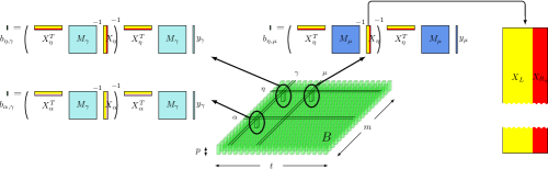
Figure 1: Interpretation of GWAS as a two-dimensional sequence of generalized least-squares problems ($b:=(X^{T}{M}^{-1}X)^{-1}X^{T}{M}^{-1}y$). GWAS with multiple phenotypes requires the solution of $m\times t$ correlated GLS problems, originating a three-dimensional object $B$ of size $m\times t\times p$. As suggested by the colors, along the $t$ direction the covariance matrix $M$ and the phenotype $y$ vary, while the design matrix $X$ does not; conversely, in the $m$ direction, $M$ and $y$ are fixed, while $X$ varies. The colors also hint at the fact that $X$ can be viewed as consisting of two parts, $X_{L}$ and $X_{R}$, where the former is constant across the entire grid and the latter changes along $m$.

2.1 Related Work

The black-box nature of traditional numerical libraries limits them to offering routines for the zero-dimensional case, a point in the grid, and use such kernel repeatedly for each problem in the sequence. As discussed previously, such an approach is absolutely unviable. Instead, GWAS-specific tools, such as GenABEL and FaST-LMM, incorporate and exploit knowledge specific to the application. However, these tools still present limitations in all three of the GWAS challenges: 1) they are tailored for a one-dimensional sequence of problems, individual columns of Fig. 1; for the solution of the entire two-dimensional grid they only offer the possibility of repeatedly using their one-dimensional solver. From a multi-trait GWAS perspective, this still represents a black box approach, missing opportunities for further computation reuse; 2) they incorporate rudimentary out-of-core mechanisms that lack the overlapping of data transfers with computation, thus incurring a considerable overhead; and 3) they attain only poor scalability.

2.2 Terminology

Here we give a brief description of the acronyms used throughout the paper.

• GWAS: Genome-Wide Association Studies.

• GLS: Generalized Least-Squares problems.

• GenABEL: A framework for statistical genomics, including one of the most widely used packages to perform gwas.

• gwfgls: GenABEL’s state-of-the-art routine for GWAS.

• fast-lmm: The most recent high-performance tool for GWAS.

• mt-gwas: our novel solver for multi-trait GWAS.

Additionally, we will reference many times

• BLAS (Basic Linear Algebra Subprograms) [Dongarra et al. (1990)], and

• LAPACK (Linear Algebra PACKage),

as the de-facto standard libraries for high-performance dense linear algebra computations.

3 The multi-trait GWAS algorithm

mt-gwas, a novel algorithm for multi-trait GWAS is introduced: First we describe a simplified version that solves one single GLS instance, and then show how the algorithm can be tailored for Eqs. (1) and (2), the solution of the whole GWAS. We stress that while mt-gwas is suboptimal for the solution of one single GLS, it exploits the specific structure and properties of the full problem, and dramatically reduces its computational complexity, thus achieving remarkable speedups.

3.1 Single-instance

The fastest approach for Eq. (1) involves computing the Cholesky factorization of the matrix $M$ [Paige (1979)], for a cost of $\frac{n^{3}}{3}$ flops. In the context of GWAS, in which $M$ varies with the index $j$ (Eq. (2)), such a factorization has to be performed $t=10^{4}$–$10^{5}$ times, thus originating a computational bottleneck. Instead, the main idea behind mt-gwas is to take advantage of the fact that $M$ results from scaling and shifting the matrix $\Phi$, which remains constant for all $i$’s and $j$’s. Then, computing the eigendecomposition $Z\Lambda Z^{T}=\Phi$ ($Z$ orthogonal, $\Lambda$ diagonal),

$$M_{j}: =\sigma^{2}_{j}(h^{2}_{j}Z\Lambda Z^{T}+(1-h^{2}_{j})I)$$

$$=ZD_{j}Z^{T},\ \ \rm{where}\ \ D_{j}=\sigma^{2}_{j}(h^{2}_{j}\Lambda+(1-h^{2}_{j})I).$$

While the eigendecomposition is much more expensive than the Cholesky factorization, $\frac{10}{3}n^{3}$ vs. $\frac{n^{3}}{3}$ flops, it allows us to express $M_{j}^{-1}$, for any $j$, with only $O(n)$ additional flops:

$$M_{j}^{-1}=ZD_{j}^{-1}Z^{T}.$$

After this initial step, Eq. (1) can be rewritten as

$$b_{ij}:=(X_{i}^{T}ZD_{j}^{-1}Z^{T}X_{i})^{-1}X_{i}^{T}ZD_{j}^{-1}Z^{T}y_{j}.$$

Since $M_{j}$ is SPD, its eigenvalues $D_{j}$ are all positive. Accordingly, the algorithm may take advantage of the symmetry of the expression $X_{i}^{T}ZD_{j}Z^{T}X_{i}$, and save computations. This is accomplished by computing the inverse of the square root of each entry of $D_{j}$ ($K_{j}:=D^{-\frac{1}{2}}_{j})$, resulting in

$$b_{ij}:=(X_{i}^{T}ZK_{j}K^{T}_{j}Z^{T}X_{i})^{-1}X_{i}^{T}ZK_{j}K^{T}_{j}Z^{T}y_{j}.$$

Next, the products $X^{\prime}_{i}:=Z^{T}X_{i}$ and $y^{\prime}_{j}:=Z^{T}y_{j}$ are computed

$$b_{ij}:=(X^{\prime T}_{i}K_{j}K^{T}X^{\prime}_{i})^{-1}X^{\prime T}_{i}K_{j}K^{T}y^{\prime}_{j},$$

and also $W_{ij}:=K^{T}_{j}X^{\prime}_{i}$ and $v_{j}:=K^{T}_{j}y^{\prime}_{j}$

$$b_{ij}:=(W^{T}_{ij}W_{ij})^{-1}W^{T}_{ij}v_{j}.$$

What remains is an ordinary least-squares problem. Numerical considerations allow us to safely rely on forming $S_{ij}:=W^{T}_{ij}W_{ij}$ without incurring instabilities. The algorithm completes by computing $b_{ij}:=W^{T}_{ij}v_{j}$ and solving the corresponding SPD linear system $b_{ij}:=S_{ij}^{-1}b_{ij}$. mt-gwas is detailed in Algorithm 1.

Algorithm 1: mt-gwas for the solution of a single instance of the generalized least-squares problem.

⬇

1 $Z\Lambda Z^{T}=\Phi$

2 $D_{j}:=\sigma^{2}_{j}(h^{2}_{j}\Lambda+(1-h^{2}_{j})I)$

3 $K_{j}K_{j}^{T}=D_{j}^{-\frac{1}{2}}$

4 $X^{\prime}_{i}:=Z^{T}X_{i}$

5 $y^{\prime}_{j}:=Z^{T}y_{j}$

6 $W_{ij}:=K_{j}^{T}X^{\prime}_{i}$

7 $v_{j}:=K_{j}^{T}y^{\prime}_{j}$

8 $S_{ij}:=W_{ij}^{T}W_{ij}$

9 $b_{ij}:=W_{ij}^{T}v_{j}$

10 $b_{ij}:=S_{ij}^{-1}b_{ij}$

3.2 Tailoring for the two-dimensional sequence

We now discuss how to extend Algorithm 1 for the solution of the two-dimensional sequence of GLSs specific to GWAS. The general objective is to identify opportunities for reusing partial calculations across different problems, in order to reduce the overall cost.

As a first step, we expose further application-specific knowledge: between any two matrices $X_{i_{1}}$ and $X_{i_{2}}$, only the right portion changes. In Algorithm 2, every appearance of $X_{i}$ is replaced with its partitioned counterpart $(X_{L}\;|\;X_{R_{i}})$, and the partitioning is propagated. The subscripts $L$, $R$, $T$, and $B$ stand for $L$eft, $R$ight, $T$op, and $B$ottom, respectively. Since $S$ is symmetric, the star in the top-right quadrant indicates the transpose of $S_{BL_{ij}}$, and this quadrant does not need to be either stored or computed. This intricate refinement of the algorithm is absolutely necessary to expose for each operand, which portion varies along which dimension.

Algorithm 2: Single-instance version of mt-gwas; the structure of $X_{i}$ is exposed.

⬇

1 $Z\Lambda Z^{T}=\Phi$

2 $D_{j}:=\sigma^{2}_{j}(h^{2}_{j}\Lambda+(1-h^{2}_{j})I)$

3 $K_{j}K_{j}^{T}=D_{j}^{-\frac{1}{2}}$

4 $(X^{\prime}_{L}\;|\;X^{\prime}_{R_{i}}):=Z^{T}(X_{L}\;|\;X_{R_{i}})$

5 $y_{j}^{\prime}:=Z^{T}y_{j}$

6 $(W_{L_{j}}\;|\;W_{R_{ij}}):=K_{j}^{T}(X^{\prime}_{L}\;|\;X^{\prime}_{R_{i}})$

7 $v_{j}:=K_{j}^{T}y_{j}^{\prime}$

8 $\left(\begin{array}[]{c | c}S_{TL_{j}}&\star\\ \hline\cr S_{BL_{ij}}&S_{BR_{ij}}\end{array}\right):=\left(\begin{array}[]{c | c}W_{L_{j}}^{T}W_{L_{j}}&\star\\ \hline\cr W_{R_{ij}}^{T}W_{L}&W_{R_{ij}}^{T}W_{R_{ij}}\end{array}\right)$

9 $\left(\begin{array}[]{c}b_{T_{j}}\\ \hline\cr b_{B_{ij}}\end{array}\right):=\left(\begin{array}[]{c}W_{L_{j}}^{T}v_{j}\\ \hline\cr W_{R_{ij}}^{T}v_{j}\end{array}\right)$

10 $b_{ij}:=S_{ij}^{-1}b_{ij}$

Next, we wrap Algorithm 2 with a double loop, corresponding to the traversal of the two-dimensional $m$-$t$ grid, and reorganize the operations, aiming at eliminating redundant computation. Both traversals of the grid —by rows (for i, for j) and by columns (for j, for i)— are provided, in Algorithms 3 and 4, respectively. We will use the latter to describe how the computation can be rearranged; the same reasoning applies to the former.

For each operation in the algorithm, the dependencies on the indices $i$ and $j$ are determined by the left-hand side operand(s). Any operation whose left-hand side does not include any subscript is invariant across the two-dimensional sequence; therefore it can be computed once and reused in every other iteration of the loops. This is the case for the eigendecomposition of $\Phi$, and the computation of $X^{\prime}_{L}$. Operations that only vary across the $t$ dimension (subscript $j$), are performed once per iteration over $t$ —the outer loop— and reused across the iterations over $m$ —the inner loop—. Finally, the operations labeled with $i$ or $i,j$ are placed in the innermost loop.

Algorithm 3: Solution of the two-dimensional grid of GLS problems depicted in Fig. 1. Traversal by rows.

⬇

1 $Z\Lambda Z^{T}=\Phi$

2 $X^{\prime}_{L}:=Z^{T}X_{L}$

3 for 1 $\leq$ i $\leq$ m

4 $X^{\prime}_{R_{i}}:=Z^{T}X_{R_{i}}$

5 for 1 $\leq$ j $\leq$ t

6 $D_{j}:=\sigma^{2}_{j}(h^{2}_{j}\Lambda+(1-h^{2}_{j})I)$

7 $K_{j}K_{j}^{T}=D_{j}^{-\frac{1}{2}}$

8 $y_{j}^{\prime}:=Z^{T}y_{j}$

9 $W_{L_{j}}:=K_{j}^{T}X^{\prime}_{L}$

10 $W_{R_{ij}}:=K_{j}^{T}X^{\prime}_{R_{i}}$

11 $v_{j}:=K_{j}^{T}y_{j}^{\prime}$

12 $S_{TL_{j}}:=W_{L_{j}}^{T}W_{L_{j}}$

13 $S_{BL_{ij}}:=W_{R_{ij}}^{T}W_{L_{j}}$

14 $S_{BR_{ij}}:=W_{R_{ij}}^{T}W_{R_{ij}}$

15 $b_{T_{j}}:=W_{L_{j}}^{T}v_{j}$

16 $b_{B_{ij}}:=W_{R_{ij}}^{T}v_{j}$

17 $b_{ij}:=S_{ij}^{-1}b_{ij}$

Algorithm 4: Solution of the two-dimensional grid of GLS problems depicted in Fig. 1. Traversal by columns.

⬇

1 $Z\Lambda Z^{T}=\Phi$

2 $X^{\prime}_{L}:=Z^{T}X_{L}$

3 for 1 $\leq$ j $\leq$ t

4 $D_{j}:=\sigma^{2}_{j}(h^{2}_{j}\Lambda+(1-h^{2}_{j})I)$

5 $K_{j}K_{j}^{T}=D_{j}^{-\frac{1}{2}}$

6 $y_{j}^{\prime}:=Z^{T}y_{j}$

7 $W_{L_{j}}:=K_{j}^{T}X^{\prime}_{L}$

8 $v_{j}:=K_{j}^{T}y_{j}^{\prime}$

9 $S_{TL_{j}}:=W_{L_{j}}^{T}W_{L_{j}}$

10 $b_{T_{j}}:=W_{L_{j}}^{T}v_{j}$

11 for 1 $\leq$ i $\leq$ m

12 $X^{\prime}_{R_{i}}:=Z^{T}X_{R_{i}}$

13 $W_{R_{ij}}:=K_{j}^{T}X^{\prime}_{R_{i}}$

14 $S_{BL_{ij}}:=W_{R_{ij}}^{T}W_{L_{j}}$

15 $S_{BR_{ij}}:=W_{R_{ij}}^{T}W_{R_{ij}}$

16 $b_{B_{ij}}:=W_{R_{ij}}^{T}v_{j}$

17 $b_{ij}:=S_{ij}^{-1}b_{ij}$

As the reader might have noticed, the algorithm still performs redundant computations: Lines 6–9, 11–12, and 15 in Algorithm 3 and line 12 in Algorithm 4 depend only on the dimension traversed by the inner loop, and are therefore recomputed at each iteration of the outer loop. This flaw can be resolved by precomputing the quantities outside of the double loop, and then accessing them from within the loops. While mathematically and algorithmically possible, the approach poses practical constraints on Algorithm 3, as it would require a fairly large amount of extra storage. The solution is instead applicable in Algorithm 4: The operation $X^{\prime}_{R_{i}}:=Z^{T}X_{R_{i}}$ may overwrite $X_{R_{i}}$, making the size of temporary storage negligible. Let us stress the significance of this improvement: by avoiding redundant calculations, Algorithm 4 saves $2tmn^{2}$ flops, thus drastically lowering the cost with respect to the other state-of-the-art algorithms, and eliminates the main computation bottleneck. Henceforth, Algorithm 4 is our algorithm of choice.

Practical considerations allow us for one more optimization. Notice that operation $X^{\prime}_{R_{i}}:=Z^{T}X_{R_{i}}$ is performed independently for each $X_{R_{i}}$, resulting in $m$ matrix-vector multiplications. Instead, these matrix-vector operations may be bundled together in a single large matrix-matrix product, known to be a much more efficient operation. Similar reasoning applies to the operation at line 6, $y^{\prime}_{j}:=Z^{T}y_{j}$.

mt-gwas, the final algorithm that includes all these optimizations, is provided in Algorithm 5. There, $\mathcal{X}_{R}$ and $\mathcal{Y}$ are used to represent the collection of all $X_{R}$’s and all $y$’s, respectively: $\mathcal{X}_{R}=(X_{R_{1}}\;|\;X_{R_{2}}\;|\;\ldots\;|\;X_{R_{m}})$ and $\mathcal{Y}=(y_{1}\;|\;y_{2}\;|\;\ldots\;|\;y_{t})$. The second and third columns indicate, respectively, for each individual operation, the corresponding BLAS or LAPACK routine and its associated cost.

Algorithm 5: mt-gwas

⬇

1$\mathcal{B}:=$ mt-gwas( $X_{L}$, $\mathcal{X}_{R}$, $\mathcal{Y}$, $h^{2}_{j}$, $\sigma^{2}_{j}$, $\Phi$ )

2 $Z\Lambda Z^{T}=\Phi$ (eigendec) $\frac{10}{3}n^{3}$

3 $X^{\prime}_{L}:=Z^{T}X_{L}$ (gemm) $2n^{2}(p-1)$

4 $\mathcal{X}_{R}^{\prime}:=Z^{T}\mathcal{X}_{R}$ (gemm) $2n^{2}m$

5 $\mathcal{Y}^{\prime}:=Z^{T}\mathcal{Y}$ (gemm) $2n^{2}t$

6 for 1 $\leq$ j $\leq$ t

7 $D_{j}:=\sigma^{2}_{j}(h^{2}_{j}\Lambda+(1-h^{2}_{j})I)$ (scalar-op) $2n$

8 $K_{j}K_{j}^{T}=D_{j}^{-\frac{1}{2}}$ (scalar-op) $2n$

9 $W_{L_{j}}:=K_{j}^{T}X^{\prime}_{L}$ (scalar-op) $(p-1)n$

10 $v_{j}:=K_{j}^{T}y_{j}^{\prime}$ (scalar-op) $n$

11 $S_{TL_{j}}:=W_{L_{j}}^{T}W_{L_{j}}$ (syrk) $(p-1)^{2}n$

12 $b_{T_{j}}:=W_{L_{j}}^{T}v_{j}$ (gemv) $2(p-1)n$

13 for 1 $\leq$ i $\leq$ m

14 $W_{R_{ij}}:=K_{j}^{T}X^{\prime}_{R_{i}}$ (scalar-op) $n$

15 $S_{BL_{ij}}:=W_{R_{ij}}^{T}W_{L_{j}}$ (gemv) $2(p-1)n$

16 $S_{BR_{ij}}:=W_{R_{ij}}^{T}W_{R_{ij}}$ (dot) $2n$

17 $b_{B_{ij}}:=W_{R_{ij}}^{T}v_{j}$ (dot) $2n$

18 $b_{ij}:=S_{ij}^{-1}b_{ij}$ (posv) $O(p^{3})$

3.3 Computational cost

Let us now compare the computational cost of mt-gwas with that of the aforementioned alternatives: LAPACK, FaST-LMM, and GenABEL. To this end, we recall the size of the input and output operands:

• $X_{L}\in R^{n\times(p-1)}$,

• $\mathcal{X}_{R}\in R^{n\times m}$,

• $\mathcal{Y}\in R^{n\times t}$,

• $h^{2}_{j}$, $\sigma^{2}_{j}\in R$,

• $\Phi\in R^{n\times n}$,

• $\mathcal{B}\in R^{m\times t\times p}$.

Typical values for these dimensions are:

• $10^{3}\leq n\leq 10^{4}$,

• $2\leq p\leq 20$,

• $10^{6}\leq m\leq 10^{8}$,

• $10^{4}\leq t\leq 10^{5}$.

The asymptotical cost of mt-gwas (see third column in Algorithm 5) is $O(n^{3}+mn^{2}+tn^{2}+tmpn)$. Since in a typical scenario for multi-trait GWAS $m$ and $t$ are much larger than $n$, the dominating factor is $O(tmpn)$. By contrast, the cost for the traditional library approach of LAPACK, which optimizes for a single GLS ($O(n^{3})$) and uses it for each point in the two-dimensional grid, is $O(tmn^{3})$; the cost for state-of-the-art tools —FaST-LMM and GenABEL—, which optimize for a one-dimensional analysis ($O(mn^{2})$) and use it for each column in Fig. 1, is $O(tmn^{2})$.

Table 1 collects the mentioned costs together with the ratio with respect to mt-gwas. The message is clear: No matter how optimized a solver for a single GLS or for a one-dimensional analysis is, it cannot compete with a solver specifically tailored for the entire multi-trait analysis.

mt-gwas exploits the specific structure of the operands and the correlation among GLSs, and lowers the cost of the best existing methods by a factor of $O(\frac{n}{p})$. For a problem of size $n=1{,}000$, $p=4$ and large $m$ and $t$, we can expect mt-gwas to be around two orders of magnitude faster than fast-lmm and gwfgls.

	Computational cost	Ratio over mt-gwas
ylapacky	$O(tmn^{3})$	$O(\frac{n^{2}}{p})$
ygwfglsy	$O(tmn^{2})$	$O(\frac{n}{p})$
yfast-lmmy	$O(tmn^{2})$	$O(\frac{n}{p})$
ymt-gwas y	$O(tmnp)$	$1$

Table 1: Asymptotic cost of each of the discussed approaches to multi-trait GWAS. The ratio over mt-gwas illustrates the impact of exploiting increasing levels of correlation within GWAS. mt-gwas improves the cost of state-of-the-art tools by a factor of $O(\frac{n}{p})$.

4 Out-of-core: Analysis of computation and data transfers

In addition to the formidable computational complexity, GWAS poses a second challenge: the management of large datasets. In the prospective scenario in which $m=36{,}000{,}000$, $t=300{,}000$, and $n=10{,}000$, the size of input and output data amounts to tens and hundreds of terabytes, respectively. Current analyses already involve the processing and generation of few terabytes of data.

Obviously, present shared-memory architectures are not equipped with such an amount of main memory; the size of the datasets thus becomes a limiting factor. In order to overcome this limitation, we turn our attention to out-of-core algorithms [Toledo (1999), Grimes (1988), Agullo et al. (2007)]. The goal is to design an algorithm that makes an effective use of the available input/output (I/O) mechanisms, to deal with data sets as large as the available secondary storage, and to minimize the overhead due to data transfers.

In the general case, the operands $\mathcal{X}_{R}$, $\mathcal{Y}$, and $\mathcal{B}$ are too large to fit in main memory and need to be streamed from disk to memory and vice versa. A naive approach, which too often becomes the choice for actual implementations, is sketched in Algorithm 6. The algorithm loads one $y$ and one $X_{R}$ and stores one $b$ at a time, resembling an unblocked algorithm. A quick study of the computation and data transfers suffices to understand the poor quality of the approach. Let us assume the following problem sizes: $n=1{,}000$, $p=4$, $m=10^{6}$, and $t=10^{5}$. On the one hand, this data set requires the performance of approximately 1.1 petaflops; at a rate of 25 GFlops/sec (see Sections 5 and 6 for details), it would complete in about 12 hours. On the other hand, loading $t$ times the whole operand $\mathcal{X}_{R}$ ($n\times m\times t\times 8$, assume 8 byte, double precision, data) already causes 800 TBs of traffic between disk and main memory. At a peak bandwidth of 2 GB/sec, which is by no means reached due to the small size of the transfers, the data movement alone takes 111 hours, about 10 times more than the time spent in actual computation. In order to attain an efficient out-of-core design, one has to a) study how different parameters affect the ratio between computation and data movement, aiming at reducing the latter, and b) use techniques for overlapping I/O with computation, thus leading to a complete elimination of I/O overhead.

Algorithm 6: Sketch of a naive out-of-core scheme for mt-gwas.

⬇

1$\mathcal{B}:=$ mt-gwas( $X_{L}$, $\mathcal{X}_{R}$, $\mathcal{Y}$, $h^{2}_{j}$, $\sigma^{2}_{j}$, $\Phi$ )

2 [$\ldots$]

3 for 1 $\leq$ j $\leq$ t

4 load $y_{j}$

5 [$\ldots$]

6 for 1 $\leq$ i $\leq$ m

7 load $X_{R_{i}}$

8 [$\ldots$]

9 store $b_{ij}$

The key behind a drastic reduction of data movement is data reuse; this is commonly attained by blocked algorithms or, in the context of out-of-core, tiled algorithms. The idea consists in loading not one single $y$ and $X_{R}$ at a time, but many of them, in a chunk or slab; once loaded in memory, each of the elements in the slabs can be used repeatedly. Following this approach, the cost of an expensive operation such as a disk-memory transfer, is amortized by performing many more arithmetic operations per transferred element.

The ratio of computation over transferred data

$$r\equiv\frac{\text{\tt\# flops}}{\text{\tt data\_to\_load + data\_to\_store}}$$ (3)

gives an approximate idea of the potential for the minimization of the impact of the data transfers. Since the time for loading an element from disk is much larger than performing a scalar operation, large ratios are desired. When applied to a concrete situation, the ratio $r$ exposes a number of parameters or degrees of freedom that may be adjusted to improve the ratio. In the context of Algorithm 5, these degrees of freedom are the number of $y$’s and $X_{R}$’s loaded at a time.

The above ratio may be extended to incorporate the concept of overlapping. For the algorithm to completely hide the I/O under computation, the time spent in computation must be larger than the time for loading and storing data. Hence, the inequality

$$\text{\tt computation\_time}>\text{\tt IO\_time}$$

must hold. The inequality may be refined as

$$\frac{\text{\tt\# flops}}{\text{\tt\# flops/sec}}>\frac{\text{\tt data\_to\_load + data\_to\_store}}{\text{\tt IO\_bandwidth}}.$$ (4)

Inequality (4) enables the identification of (ranges of) values for the aforementioned degrees of freedom, so that a perfect overlapping is achieved.

As an overlapping out-of-core mechanism we choose the so-called double-buffering. In short, to deploy double-buffering, main memory is divided into two workspaces. Each workspace contains buffers, one per operand to be streamed; in this case, two buffers for the input operands $\mathcal{X}_{R}$ and $\mathcal{Y}$, and one for the output stream $\mathcal{B}$. At a given iteration over the streams, one workspace is used for computation, while the other one is used for downloading previous results and uploading data for the next iteration. After each iteration, the workspaces swap roles. For more details, we refer the reader to [Fabregat-Traver et al. (2012)].

The rest of this section is dedicated to the analysis of the computation and data transfer required by Algorithm 5. During the analysis we expose the degrees of freedom, and provide the specific constraints they must satisfy.

4.1 Preloops: Single sweep over the input streams

We logically divide Algorithm 5 in two sections: 1) preloops —lines 1 to 4—, and 2) loops —lines 5 to 17—. In the preloops, the operations at lines 1 and 2 involve operands that fit in main memory; they are therefore computed through direct calls to the corresponding BLAS and LAPACK routines. On the contrary, the two matrix products at lines 3 and 4 involve the operands $\mathcal{X}_{R}$ and $\mathcal{Y}$, which reside on disk, and must therefore be performed in a streaming fashion.

The approach to compute $\mathcal{X}^{\prime}_{R}:=Z^{T}\mathcal{X}_{R}$ (line 4), and equivalently $\mathcal{Y}^{\prime}:=Z^{T}\mathcal{Y}$ (line 3), consists in a traversal over the stream $\mathcal{X}_{R}$ in slabs containing $nb$ $X_{R}$’s, where the optimal value for $nb$ is to be estimated. At every step over the stream (Fig. 2(a)), the algorithm

1. loads $nb$ $X_{R}$’s, each of them of size $n$, i.e., $n\times nb$ elements;

2. stores $nb$ $X^{\prime}_{R}$’s, each of them also of size $n$; and

3. performs $2\times n^{2}\times nb$ flops, corresponding to the matrix product $\mathcal{X}^{\prime}_{R_{i}}:=Z^{T}\mathcal{X}_{R_{i}}$.

The ratio of computation over data movement is

$$\frac{2\times n^{2}\times nb}{(n\times nb)+(n\times nb)}\quad\equiv\quad n.$$

For typical values of $n$ —from one thousand to tens of thousands—, such a ratio shows great potential for perfect overlapping.

Notice that, even though the ratio is independent of the value of $nb$, two quantities in (4) are influenced by this parameter: the performance of gemm (# flops/sec), and the data transfer rate (IO_bandwidth). The objective for both quantities is clear: One wants to maximize them both, to minimize execution time and I/O time. The constraint to satisfy is

$$\frac{2\times n^{2}\times nb}{\text{\tt\# flops/sec}}>\frac{2\times n\times nb\times\text{\tt sizeof(datatype)}}{\text{\tt IO\_bandwidth}},$$ (5)

which simplifies to

$$\frac{n}{\text{\tt\# flops/sec}}>\frac{\text{\tt sizeof(datatype)}}{\text{\tt IO\_bandwidth}}.$$ (6)

Since these quantities are specific to the architecture and the problem, we defer their evaluation to Sec. 6, where the experimental setup is defined.

4.2 Loops: Cross product of the input streams

The analysis and application of double-buffering to the second section of the algorithm requires a deeper discussion. Instead of a single sweep through the streams, this section operates on every pair ($X_{R_{i}}$, $y_{j}$) of data, i.e., a “cross product” of the input streams $\mathcal{X}_{R}$ and $\mathcal{Y}$. The problem can be translated into how the object $\mathcal{B}$ is built. In view of the impossibility of fitting the entire data set in memory, the problem of computing $\mathcal{B}$ is decomposed into the computation of smaller parts or tiles (Fig. 2(b)). Let us assign each tile the size $mb\times tb$, where $mb$ and $tb$ are the number of $X_{R}$’s and $y$’s processed, respectively. Henceforth we concentrate on determining adequate values for these two parameters.

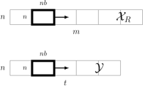
(a) Single-sweep traversal of the streams $\mathcal{X}_{R}$ and $\mathcal{Y}$ in slabs of $nb$.

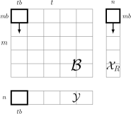
(b) Computation of object $\mathcal{B}$ of size $m\times t$ decomposed into tiles of size $(mb\times tb)$. Traversal by columns.

Figure 2: Meaning of the degrees of freedom in the application of double-buffering to mt-gwas.

As for the first section of the algorithm, the goal is to achieve a perfect overlapping of I/O with computation. To this end, we must once more study the ratio of computation over data movement as a function of the tile size. To compute a tile, the algorithm must load $(mb\times n)+(tb\times n)$ elements, corresponding to the loading of a slab of $\mathcal{X}_{R}$’s and a slab of $\mathcal{Y}$’s, and store $(mb\times tb\times p)$ elements, corresponding to a slab of $\mathcal{B}$. Per tile, $O(mb\times tb\times n\times p)$ flops are performed, for a ratio of

$$\frac{O(mb\times tb\times p\times n)}{(mb\times n+tb\times n)+(mb\times tb\times p)}.$$

In Section 3.2 we deduced that a traversal by columns of the grid depicted in Fig. 1, is favorable in terms of computational cost and temporary storage. Hence, the algorithm will load a slab of $\mathcal{Y}$’s and reuse it for all $\mathcal{X}_{R}$’s. Consequently, the cost of loading the slab of $\mathcal{Y}$’s can be neglected, and the ratio simplifies to

$$r=\frac{O(tb\times p\times n)}{n+tb\times p}.$$

This ratio $r$ is independent of the value $mb$. Intuitively, if $mb$ is multiplied by 2, both the amount of computation within the tile and the required I/O are doubled (twice the number of $X_{R}$’s are loaded and twice the number of $b_{ij}$’s are computed and stored). On the contrary, the ratio grows monotonically with $tb$. For the sake of clarity, we illustrate in Fig. 3 the behavior of $r$ as a function of $tb$. For $tb=1$, $r$ is $O(p)$; the ratio rapidly grows with $tb$ until it reaches a value of about $2n$, from where the growth is much smaller.

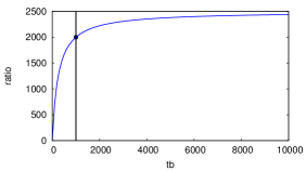
Figure 3: Ratio of computation over data transfer for tiles of $\mathcal{B}$. The ratio is plotted as a function of $tb$, with $p=4$ and $n=1000$. The ratio is initially very low but grows rapidly to values that allow a perfect overlapping of I/O with computation.

As discussed previously, large values of the ratio are favored. Therefore, tiling along the $t$ dimension ($tb>1$) is imperative to reduce the I/O overhead.

However, since we are making use of double-buffering, we do not need to choose the largest possible $tb$; we only require $tb$ to be large enough to completely hide the overhead due to I/O. The minimum value of $tb$ leading to a perfect overlap can be determined analytically via (4). The time for computing a tile must be larger than the time for loading a slab of $\mathcal{X}_{R}$ and storing the corresponding slab of $\mathcal{B}$:

$$\frac{mb\times tb\times(5+2(p-1))\times n}{\text{\tt\# flops/sec}}>\frac{(mb\times n+mb\times tb\times p)\times\text{\tt sizeof(datatype)}}{\text{\tt IO bandwidth}}.$$

Dividing both sides by $mb$:

$$\frac{tb\times(5+2(p-1))\times n}{\text{\tt\# flops/sec}}>\frac{(n+tb\times p)\times\text{\tt sizeof(datatype)}}{\text{\tt IO bandwidth}}.$$ (7)

In Eq. (7), the values for $n$ and $p$ are given as input; the datatype is known; the hard-drive bandwidth is to be determined empirically; and the performance attained in the computation of a tile is determined when tailoring for the architecture, as discussed in Section 5. As we observed for $nb$, the parameter $mb$ does not influence the reduction of data transfer, and it has to satisfy no explicit constraint. Still, tiling along $m$ ($mb>1$) is recommended for performance reasons, as we demonstrate in Section 5.

Let us summarize the study performed in this section. We exposed and analyzed the degrees of freedom in the tiling of our algorithm: $nb$, $mb$, and $tb$. The main message of the study is that $tb$ is the key in the reduction of the data movement to make the computation feasible. Additionally, we discussed the implication of the value of all three parameters in terms of performance, and stated the two key constraints —Eqs. (6) and (7)— to be satisfied in order to completely eliminate overhead due to I/O operations.

5 Tailoring for shared-memory parallelism

Algorithm 5 (described in Sections 3 and 4) both has a lower computational complexity than all the current alternatives and eliminates the overhead due to I/O. Yet, a careful implementation is required to exploit shared-memory parallelism. In this section, we explain how to select the best-suited type of parallelism for each section of the algorithm, and outline the steps to achieve almost optimal scalability.

5.1 Preloop: Multi-threaded BLAS

The operations in the preloop section, lines 2–5, correspond to either LAPACK routines (eigendecomposition) that cast most of the computation in terms of BLAS-3 kernels, or are direct calls to BLAS-3 routines (gemm). For this class of routines, it is well known that optimized multi-threaded BLAS libraries deliver both high-performance and scalability. This is therefore the solution we adopt.

5.2 Loops: Single-threaded BLAS + OpenMP parallelism

In sharp contrast to the preloops, the computation performed within the loops, lines 6–18, maps to non-scalable BLAS-1 and BLAS-2 operations, thus making the use of multi-threaded BLAS not viable. Instead, we exploit the multi-core parallelism by utilizing a single-threaded BLAS in combination with OpenMP threads and by decomposing the computation in tasks.

In Section 4, it was shown that tiling the computation of $\mathcal{B}$ along the $t$ dimension is the key to eliminate penalties due to I/O data transfers. In this section we demonstrate that for a high-performance shared-memory implementation, it is also crucial to tile along the $m$ dimension, and discuss how to select the best tile size and shape. Furthermore, we explore different multi-threading strategies to manage the data transfers, and to split and assign computational tasks to cores; since the total number of options is daunting, here we only describe those two that we considered most promising:

1. a single master thread is responsible for the streaming of all tiles, and all threads collaborate in the computation of each tile; and

2. each thread operates on whole tiles, and is responsible for their streaming.

5.2.1 Two-dimensional tiling

If we only consider tiles of size $1\times tb$, the largest tile is of size $1\times 100{,}000$ (See Fig. 2(b), with $mb=1$ and $tb=t$). In our experimental environment with 40 threads, each thread computes a task or block of size $1\times 2{,}500$, attaining poor efficiency: 1.54% Instead, by tiling (and blocking) along $m$ as well as along $t$, efficiency increases:

1. For a tile size of $200\times 100{,}000$ with blocks of size $1\times 100{,}000$, the attained efficiency is 3.75%.

2. For a tile size of $1{,}000\times 100{,}000$ with blocks of size $100\times 100$, the efficiency raises to 6.35%.

A higher workload per thread —case a)— results in a speedup of about 2.5x; by further increasing the value of $mb$ —case b)— data locality improves, for speedups of about 4x. The benefits of using two-dimensional tiles are thus clear; it remains to determine how such tiles should be decomposed to maximize performance.

5.2.2 Estimating the best block size

Typically, as long as the tile size satisfies the constraints (6) and (4.2), one chooses $mb$ and $tb$ to maximize the RAM usage. For performance purposes, the computation of such large tiles must be split into smaller blocks to exploit both the memory hierarchy and all the available cores. The same way the tile size is chosen according to the amount of available main memory, in cache-based architectures the block size is determined according to the size of the cache memories. The challenge lies on finding the optimal block size $(mbb\times tbb)$.

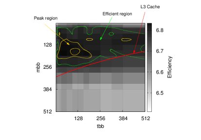
Figure 4: Study of the performance attained by different block sizes $(mbb\times tbb)$. The red line (L3 cache) delimits the blocks that fit in L3 cache —above the line—. The green region (Efficient region) includes block sizes attaining an efficiency of at least 6.7%. Most of the region fits in L3. The yellow region (Peak region) includes the most efficient blocks (efficiency above 6.8%). The fluctuation within the Peak region is less than 0.5%.

We consider blocking for the highest level of cache. Fig. 4 provides a heatmap representing the efficiency attained varying the block sizes. The red line delimits the space of block sizes that fit in the last level of cache —level 3 (L3) for the architecture used in our experiments (see Section 6 for details)—. As anticipated, the block sizes attaining higher efficiency (green line: Efficient region) lie above the red line, i.e., fit in L3 cache. Also expected is the fact that relatively large square blocks attain the highest efficiency (yellow line: Peak region).

Interestingly, we observed that inside the Peak region performance plateaus, exhibiting variations below 0.5%. This suggests that one should focus on finding this region rather than the most efficient block size. As a matter of fact, since within the Peak region the fluctuations due to the hardware and the operating system are greater than the differences in performance, it can be argued that a best block size does not even exist.

5.2.3 Work distribution

We conclude describing two possibly strategies to distribute the blocks among cores.

1. Cooperative threads (mt-gwas-ct). A common scheme for tile-based implementations of out-of-core algorithms consists of a master thread that takes care of all data transfers, and a number of spawned threads that cooperate in the computation of each tile. As Fig. 5 illustrates, each tile is divided into blocks, and these are distributed among computing threads, thus sharing the workload.

2. Independent threads (mt-gwas-it). Alternatively, work may be distributed so that each thread is responsible for the loading, computation, and downloading of its own entire tiles. As Fig. 5 illustrates, each tile is still decomposed into blocks for performance reasons.

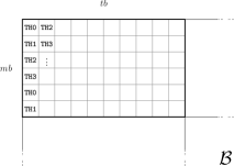
(a) Cooperative threads: A master thread loads each tile, and all spawned threads cooperate on the computation of the tile.

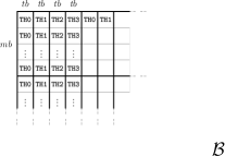
(b) Independent threads: Each thread is responsible for the loading, computation and downloading of its own tiles.

Figure 5: The two studied approaches to work distribution.

6 Experimental results

We focus now on experimental results. We compare the performance and scalability of the state-of-the art tools, fast-lmm and gwfgls, with those of the presented algorithm mt-gwas. For mt-gwas we provide results for both parallel approaches described in Section 5.2.3: mt-gwas-ct for cooperative threads, and mt-gwas-it for independent threads.

6.1 Experimental setup

All tests were run on a SMP system consisting of 8 Intel Xeon E7-4850 multi-core processors. Each processor comprises ten cores, operating at a frequency of 2.00 GHz, for a combined peak performance of 320 GFlops/sec. The system is equipped with 512GB of RAM and 4TBs of disk as secondary memory. The I/O system attains a maximum bandwidth of 2GBs/sec for data transfers of at least 2MBs.

The routines were compiled with the GNU C Compiler (gcc, version 4.4.5), and linked to a multi-threaded Intel’s MKL library (version 10.3). Our routines make use of the OpenMP parallelism provided by the compiler through a number of pragma directives. All computations were performed in double precision.

6.2 Configuring the degrees of freedom

In order to attain maximum performance, we need to estimate the most effective values for the algorithm parameters: $nb$, $mb$, $tb$, $mbb$, and $tbb$.

6.2.1 $nb$

As described in Section 4, this parameter is chosen to be greater than or equal to the minimum value that maximizes both data transfer rate and gemm’s performance. The maximum I/O bandwidth is attained for transfers of at least 2MBs; the minimum value of $nb$ to reach this size is 250 ($nb\times n\times\text{\tt sizeof(datatype)}\equiv 250\times 1000\times 8B\equiv 2$MBs). We also determined empirically that the minimum value of $nb$ to maximize gemm’s performance for 40 cores in the specified architecture is $10{,}000$ (attaining 240 GFlops/sec). Therefore, we set $nb$ to $10{,}000$. Substituting in Eq. (6), we see that we will achieve a perfect overlapping:

$$\frac{1000}{240\times 10^{9}}>\frac{8}{2\times 10^{9}}\equiv 4.17>4.$$

6.2.2 $mbb$ and $tbb$

According to the results shown in Fig. 4, we simply choose a square block size within the Peak region: $160\times 160$.

6.2.3 $mb$ and $tb$

We determined that the maximum performance attained in the computation of a tile is about 25 GFlops/sec. Substituting each variable in Eq. (7):

$$\frac{tb\times 11\times 1000}{25\times 10^{9}}>\frac{8000+tb\times 32}{2\times 10^{9}}\quad\equiv\quad tb>10.$$

Therefore, and given the chosen block size, the constraint above ($tb>10$) does not impose any restriction in our choice of tile size ($tb$ will be at least 160). In any case, we emphasize the importance of always carrying out such an analysis, as differences in performance or I/O bandwidth could lead to more restrictive constraints.

As discussed in Section 5, we choose different tile sizes for the different approaches to work distribution. In the case of mt-gwas-ct, we consider large square tiles maximizing the usage of free main memory; accordingly we choose $mb=tb=25{,}600$. For mt-gwas-it, we fix the value of $tb$ to that of the block size, i.e., $tb=tbb=160$, while for $mb$ we select a small multiple of the block size ($mb=1600$). The reason for such a small tile size is to show that our routine can achieve impressive speedups even with a limited amount of main memory, emphasizing that the only restriction for mt-gwas is the size available amount of secondary device storage. As an example, for the execution of the largest test reported in this section, which involves the processing of more than 3 terabytes of data, mt-gwas-it only required less than 2 gigabytes of memory.

6.3 Experiments

We present performance results for fast-lmm, gwfgls, mt-gwas-ct, and mt-gwas-it. At first, results for a single core are given, to highlight the speedup due to the sole improvement of the algorithm, i.e., the reduction in computational cost. Then, we compare the scalability and performance of all four algorithms, using all the available 40 cores.

In Fig. 6, we provide timings for the four routines for increasing values of $t$. The experiments were run using a single thread. The gap between the state-of-the-art routines and our novel algorithm is substantial: while fast-lmm and gwfgls would take, respectively, about 10 and 8.5 days to complete, mt-gwas-ct and mt-gwas-it reduce the execution time to 5.3 and 4.8 hours, respectively. In terms of speedups, our best routine, mt-gwas-it, is 50 and 43 times faster than fast-lmm and gwfgls, respectively. It is also worth noticing the 10% speedup of mt-gwas-it with respect to mt-gwas-ct.

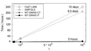
Figure 6: Performance of the single-threaded versions of the four presented routines. The problem dimensions are: $n=1{,}000$, $p=4$, and $m=100{,}000$. For $t=10{,}000$, our routines —mt-gwas-ct and mt-gwas-it— outperform the state-of-the-art tools fast-lmm and gwfgls by a factor of 50 and 43, respectively.

Scalability results are shown in Fig. 7. The figure reveals clear scalability issues in the parallel implementations of both fast-lmm and gwfgls; they achieve speedups between 1.4 and 1.6, and plateau when 16 or more cores are used. Instead, the results for our routines clearly demonstrate the benefit of carefully tailoring Algorithm 5 for large shared-memory architectures: Using all available 40 cores, mt-gwas-ct and mt-gwas-it attain speedups of 35 and 36.6, respectively. Furthermore, the trend presented by both our routines forecasts larger speedups, should more cores be available.

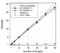
Figure 7: Scalability of mt-gwas-ct, mt-gwas-it, fast-lmm, and gwfgls. While fast-lmm and gwfgls present a mediocre scalability, our routines —mt-gwas-ct and mt-gwas-it— attain speedups of 35x and 36.6x, respectively, when using 40 threads. The problem dimensions are: $n=1{,}000$, $p=4$, $m=100{,}000$, and $t=20{,}000$.

Figure 8 presents performance results for the same four routines when using 40 threads. Here, the effects of the computational cost reduction, the perfect I/O overlapping, and a better scalability are all combined, yielding speedups of $1{,}352$ and $1{,}012$ over fast-lmm and gwfgls, respectively. The time to compute the largest presented problem, $n=1{,}000$, $p=4$, $m=10^{6}$, and $t=10^{5}$, is reduced from (unfeasible) years to 12 hours.

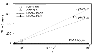
Figure 8: Performance of the multi-threaded versions. The problem dimensions are: $n=1{,}000$, $p=4$, and $m=1{,}000{,}000$. While, for $t=100{,}000$, fast-lmm and gwfgls are not viable, our routines complete in a matter of hours. The observed speedups are larger than 1000x.

7 Future Work

Multi-trait GWAS is constrained by three dimensions: $n$, ranging from $10^{3}$ to $10^{4}$, $m$, ranging from $10^{6}$ to $10^{8}$, and $t$, ranging from $10^{4}$ to $10^{5}$. The work presented in this paper allows $m$ and $t$ to grow as large as desired. On the contrary, our routines assume the operand $\Phi\in R^{n\times n}$ to fit in main memory, and thus are constrained by the size of $n$. For very large values of $n$, the problem demands a distributed-memory version of mt-gwas, and therefore requires an extension of the analysis of data transfers and work distribution undergone in this paper.

Additionally, there is an increasing demand for support of co-processors such as GPUs. While the use of GPUs was proven successful for the single-trait case ($t=1$) [Beyer (2012)], routines for the more general multi-trait case are not yet available. There, the challenge lies in writing optimized kernels for the computation within the loops, tuning for the intricate memory hierarchy of the architecture.

8 Conclusions

We addressed an extremely challenging and widespread problem in computational biology, the genome-wide association study (GWAS) with multiple traits. GWAS involves large-scale computations —petaflops— on large data sets —terabytes of data—, and the existing state-of-the-art tools are only effective in conjunction with supercomputers. In this paper we introduced mt-gwas, a novel algorithm for sequences of least-squares problems, tailored to take advantage of both application-specific knowledge and shared memory parallelism, and demonstrated that for performing the full GWAS analysis, a single multi-core node suffices.

First, we described the derivation of an algorithm that exploits all knowledge available from the application: from the specific two-dimensional sequence of generalized least-squares problems, to the special structure of the operands. By eliminating redundant computations, this algorithm lowers the asymptotical cost of state-of-the-art tools by several orders of magnitude.

Then, we discussed how to deal with large-scale datasets. In order to incorporate an out-of-core mechanism, we analyzed the ratio between data movement and computations, and derived the best tile size and shape for a perfect overlapping of data transfers with computation. This mechanism enables the processing of data sets as large as the available secondary storage, without any overhead due to I/O operations.

Finally, we tailored our algorithm for shared-memory parallel architectures. The study of the different sections of the algorithm suggested the use of a mixed parallelism: 1) multi-threaded BLAS, and 2) single-threaded BLAS and OpenMP parallelism. We empirically estimated the best size for the computational tasks, and studied two different approaches to distribute those task among threads. The resulting routines attain speedups of 35x and 36.6x on 40 cores.

By combining the effects of the computational cost reduction, the perfect I/O overlapping, and a high scalability, our routines yield, when compared to the state-of-the-art tools, a 1000-fold reduction in the time to solution. Thanks to this algorithm, analyses that were thought to be feasible only with the help of supercomputers, can now be completed in matter of a few hours with a single multi-core node.

9 Acknowledgements

Financial support from the Deutsche Forschungsgemeinschaft (German Research Association) through grant GSC 111 is gratefully acknowledged. The authors thank Matthias Petschow for discussion on the algorithms, and the Center for Computing and Communication at RWTH Aachen for the computing resources.

eceived Month Year; revised Month Year; accepted Month Year

References

- Agullo et al. (2007) Agullo, E., Guermouche, A., Num, T., Agullo, E., Guermouche, A., Graal, P., ens Lyon, L., and Bordeaux, L. 2007. Towards a parallel out-of-core multifrontal solver: Preliminary study. Research report 6120. INRIA.
- Anderson et al. (1999) Anderson, E., Bai, Z., Bischof, C., Blackford, S., Demmel, J., Dongarra, J., Du Croz, J., Greenbaum, A., Hammarling, S., McKenney, A., and Sorensen, D. 1999. LAPACK Users’ Guide, Third ed. Society for Industrial and Applied Mathematics, Philadelphia, PA.
- Aulchenko et al. (2007) Aulchenko, Y. S., Ripke, S., Isaacs, A., and van Duijn, C. M. 2007. Genabel: an R library for genome-wide association analysis. Bioinformatics 23, 10 (May), 1294–6.
- Beyer (2012) Beyer, L. 2012. Exploiting graphics accelerators for computational biology. M.S. thesis, Aachen Institute for Computational Engineering Science, RWTH Aachen.
- Bientinesi et al. (2010) Bientinesi, P., Eijkhout, V., Kim, K., Kurtz, J., and van de Geijn, R. 2010. Sparse direct factorizations through unassembled hyper-matrices. Computer Methods in Applied Mechanics and Engineering 199, 430–438.
- Blackford et al. (1997) Blackford, L. S., Choi, J., Cleary, A., D’Azevedo, E., Demmel, J., Dhillon, I., Dongarra, J., Hammarling, S., Henry, G., Petitet, A., Stanley, K., Walker, D., and Whaley, R. C. 1997. ScaLAPACK Users’ Guide. Society for Industrial and Applied Mathematics, Philadelphia, PA.
- Di Napoli et al. (2012) Di Napoli, E., Bluegel, S., and Bientinesi, P. 2012. Correlations in sequences of generalized eigenproblems arising in density functional theory. Computer Physics Communications (CPC) 183, 8 (Aug.), 1674–1682.
- Dongarra et al. (1990) Dongarra, J., Croz, J. D., Hammarling, S., and Duff, I. S. 1990. A set of level 3 basic linear algebra subprograms. ACM Trans. Math. Softw. 16, 1, 1–17.
- Fabregat-Traver et al. (2012) Fabregat-Traver, D., Aulchenko, Y. S., and Bientinesi, P. 2012. Fast and scalable algorithms for genome studies. Tech. rep., Aachen Institute for Advanced Study in Computational Engineering Science. Available at http://www.aices.rwth-aachen.de:8080/aices/preprint/documents/AICES-2012-05-01.pdf.
- Grimes (1988) Grimes, R. G. 1988. Solving systems of large dense linear equations. The Journal of Supercomputing 1, 291–299. 10.1007/BF00154340.
- (11) Hindorff, L., MacArthur, J., Wise, A., Junkins, H., Hall, P., Klemm, A., and Manolio, T. A catalog of published genome-wide association studies. Available at: www.genome.gov/gwastudies. Accessed July 22nd, 2012.
- Lauc et al. (2010) Lauc, G. et al. 2010. Genomics Meets Glycomics–The First GWAS Study of Human N-Glycome Identifies HNF1 as a Master Regulator of Plasma Protein Fucosylation. PLoS Genetics 6, 12 (12), e1001256.
- Levy et al. (2009) Levy, D. et al. 2009. Genome-wide association study of blood pressure and hypertension. Nature Genetics 41, 6 (Jun), 677–687.
- Lippert et al. (2011) Lippert, C., Listgarten, J., Liu, Y., Kadie, C. M., Davidson, R. I., and Heckerman, D. 2011. Fast linear mixed models for genome-wide association studies. Nat Meth 8, 10 (Oct), 833–835.
- Paige (1979) Paige, C. C. 1979. Fast numerically stable computations for generalized linear least squares problems. SIAM Journal on Numerical Analysis 16, 1, pp. 165–171.
- Speliotes et al. (2010) Speliotes, E. K. et al. 2010. Association analyses of 249,796 individuals reveal 18 new loci associated with body mass index. Nature Genetics 42, 11 (Nov), 937–948.
- Toledo (1999) Toledo, S. 1999. External memory algorithms. American Mathematical Society, Boston, MA, USA, Chapter A survey of out-of-core algorithms in numerical linear algebra, 161–179.