The rates and time-delay distribution of multiply imaged supernovae behind lensing clusters

Abstract

Time delays of gravitationally lensed sources can be used to constrain the mass model of a deflector and determine cosmological parameters. We here present an analysis of the time-delay distribution of multiply imaged sources behind 17 strong lensing galaxy clusters with well-calibrated mass models. We find that for time delays less than 1000 days, at $z=3.0$, their logarithmic probability distribution functions are well represented by $P(\log\Delta t)=5.3\times 10^{-4}\Delta t^{\widetilde{\beta}}/M_{250}^{2\widetilde{\beta}}$, with $\widetilde{\beta}=0.77$, where $M_{250}$ is the projected cluster mass inside 250 kpc (in $10^{14}\textrm{M}_{\odot}$), and $\widetilde{\beta}$ is the power-law slope of the distribution. The resultant probability distribution function enables us to estimate the time-delay distribution in a lensing cluster of known mass. For a cluster with $M_{250}=2\times 10^{14}\textrm{M}_{\odot}$, the fraction of time delays less than 1000 days is approximately $3\%$. Taking Abell 1689 as an example, its dark halo and brightest galaxies, with central velocity dispersions $\sigma\geqslant 500\ \textrm{km}\ \textrm{s}^{-1}$, mainly produce large time delays, while galaxy-scale mass clumps are responsible for generating smaller time delays. We estimate the probability of observing multiple images of a supernova in the known images of Abell 1689. A two-component model of estimating the supernova rate is applied in this work. For a magnitude threshold of $m_{\textrm{AB}}=26.5$, the yearly rate of Type Ia (core-collapse) supernovae with time delays less than 1000 days is $0.004\pm 0.002$ ($0.029\pm 0.001$). If the magnitude threshold is lowered to $m_{\textrm{AB}}\sim 27.0$, the rate of core-collapse supernovae suitable for time delay observation is $0.044\pm 0.015$ per year.

1 Introduction

An object in our universe, such as a galaxy or a galaxy cluster, could bend light rays passing it and act as a lens to magnify or demagnify sources behind it [1]. This effect is known as gravitational lensing and has been developed into a powerful cosmological tool in recent decades [2] [3] [4] [5]. With the help of gravitational lensing, we can observe distant galaxies behind galaxy clusters which would otherwise be too faint to be observed, and analyze their properties. We can also measure the cosmological parameters that describe the geometry and the expansion rate of the universe [6] [7]. In addition, we can analyze the total mass distribution in lensing galaxy clusters [8], regardless of the differences between luminous and dark matter [9].

In strong gravitational lensing systems, multiple images are produced. Light travels along the stationary paths between two points in space time. A massive object, like a galaxy or cluster of galaxies located along the light path, in general affects and perturbs the light trajectory [10]. When lensed by a galaxy or a cluster of galaxies, light emitted by a source may travel along different light paths and be observed as different multiple images. Light from these images is received at different times. Thus, multiple images have different arrival times to the observer. The difference of arrival times between multiple images of the same source is called the time delay.

So far, time delays have been studied and applied in many ways: to constrain the Hubble parameter $H_{0}$ [11] [12] [13]; to study the galaxy mass profile with Monte Carlo simulations [14]; to measure the cosmological parameter $w$ [15] [16] [17] [18] [13]; to improve the mass models of galaxies with the time delays of quasars [19].

Compared to quasars, light curves of type Ia supernovae (SNe Ia) evolve regularly with time, and have been extensively studied [20] [21]. Hence, they are potentially very useful as standard sources for constraining time delays in gravitational lens systems. In principle, they can also be used to constrain the Hubble constant through the measurement of the time delays [22]. SNe Ia play a key role as standard candles in distance measurements on cosmological scales. Supernovae provide direct evidence that the low-redshift universe is accelerating [23] [24] [25]. They act as the primary sources of heavy elements and potentially dust in the universe [26]. However, there is still debate on the progenitor models of SNe Ia [21] [27]. There are two major progenitor scenarios to explain the mechanism of Type Ia progenitor. In the single degenerate model [28], a carbon-oxygen white dwarf accretes mass from a companion star, a subgiant, a helium star or a red giant, and reaches the Chandrasekhar mass limit, resulting in a thermonuclear explosion [29] [30]. In the double degenerate scenario [31], two white dwarfs merge, approach the Chandrasekhar mass limit, and ignite. Recently, a third model gives another explanation of the possible SN progenitor scenarios. Instead of accreting the mass to the Chandrasekhar mass limit, the detonation ignites to the accreted He shell of one white dwarf, then the detonation shock wave comes to the core or near the center, and a second detonation happens [32] [33] [34].

The rate of supernovae (SNR) reflect their formation mechanism. For example, core-collapse SNe (Type II and Ibc supernovae) arising from massive stars help us trace the star formation and may be used to constrain the star formation rate (SFR) [35]. A well established model of estimating the SNR for Ia SNe ($\textrm{SNR}_{\textrm{Ia}}$) is a “two-component”  model [36] [37] [38], with one component dependent on the recent star formation in the host galaxy and the other component dependent on the host stellar mass. The SN type Ia rate is a combination of these two components. The $\textrm{SNR}_{\textrm{Ia}}$ at intermediate redshift has been constrained using the SDSS-II dataset to $z\leqslant 0.12$ [39], and extended analysis to $z<0.3$ [40]. At high redshift, the SN Ia rate is also tested and constrained, using the SNLS dataset to $z\thickapprox 0.5$ [41] and $0.1\leq z\leq 1.1$ [42], the HST/GOODS survey up to $z<1.8$ [43] [44], and the Subaru Deep Field (SDF) to $z<2$ [45]. The core-collapse supernova rate is also tested and estimated up to $z\sim 0.7$, using the GOODS survey. With these data and the SNR model, we can estimate the lensed SNR in a cluster lensing system [46].

The aim of this paper is to (1) develop a general function to describe the time-delay distributions in gravitational lensing systems; (2) estimate the lensed SNR as a function of time delay and magnitude in Abell 1689 to assess the feasibility of constraining mass models and cosmological parameters with lensed supernovae observationally.

The outline of the paper is as follows. In section 2, we develop a theoretical formalism for describing the time-delay distribution. The analysis and discussion of parameters for the distribution function are developed in section 3. In section 4, we model time-delay distributions of 17 massive lensing clusters. We analyze and fit the parameters of the distribution function, based on the results from modeling. In section 5, using the “two-component”  model, we calculate the probability of observing supernovae in 35 known multiply imaged galaxies behind Abell 1689. Finally, we summarize our investigation and discuss future prospects in section 6. Throughout this paper, we assume a cosmological model with $\Omega_{m}=0.3,\Omega_{\Lambda}=0.7,h=0.7$. Magnitudes are in the AB system.

2 Time delay theory

A light ray is deflected when it passes a cosmic massive object. In a lensing system, the light path from the source to the observer is changed according to the gravitational field near the lens. In the case of a multiple image system, lensing generally causes a difference in the arrival time of a galaxy image pair and hence generates a time delay. The time delay, $\Delta t$, can be calculated as [10]

$$c\Delta t(y)=\xi^{2}_{0}\frac{D_{\textrm{OS}}}{D_{\textrm{OL}}D_{\textrm{LS}}}(1+z_{L})[\phi(x_{1},y)-\phi(x_{2},y)],$$ (2.1)

where $\xi_{0}=4\pi(\frac{\sigma_{v}}{c})^{2}\frac{D_{\textrm{OL}}D_{\textrm{LS}}}{D_{\textrm{OS}}}$ is the characteristic length scale in the lens plane. Here $\sigma_{v}$ is the value of an effective velocity dispersion, $D_{\textrm{OS}}$ is the angular diameter distance between the observer and the source, $D_{\textrm{OL}}$ is the angular diameter distance between the observer and the lens, $D_{\textrm{LS}}$ is the angular diameter distance between the lens and the source, and $z_{L}$ is the lens redshift. We denote the image position in the lens plane by $\bm{\xi}$ and the source position in the source plane by $\bm{\eta}$. Here $y=|\bm{\eta}|/\eta_{0}$, is the source position in the source plane, with $\eta_{0}=\frac{\xi_{0}D_{\textrm{OS}}}{D_{\textrm{OL}}}$ being the maximal distance to the caustic line. We define $x_{i}(i=1,2)$ as two image positions in the lens plane with $x=|\bm{\xi}|/\xi_{0}$. Here $x,y$ are dimensionless vectors. The Fermat potential is defined as $\phi(x_{i},y)(i=1,2)$. For a two-image system, the larger the difference of their Fermat potentials, the larger time delay they will generate. The Fermat potential $\phi(x,y)$ can also be described by the lensing potential $\varphi(x)$ [47],

$$\phi(x,y)=\frac{(x-y)^{2}}{2}-\varphi(x).$$ (2.2)

We assume spherically symmetric lenses in what follows.

Generally, for a lens with density distribution $\rho\varpropto r^{-\delta}$, the time delay can be expanded as [8] [48]

$$\Delta t(\delta)\approx(\delta-1)\Delta t_{\textrm{SIS}}\left[1-\frac{(2-\delta)^{2}}{12}\left(\frac{\Delta r}{\langle r\rangle}\right)^{2}\cdots\right],$$ (2.3)

where $\Delta t_{\textrm{SIS}}$ represents the time delay for the Singular Isothermal Sphere (SIS; $\delta=2$), and $\langle r\rangle=(r_{i}+r_{j})/2$. If the term $\frac{\Delta r}{\langle r\rangle}$ is small, the higher order terms can be ignored.

For real clusters, tidal perturbations from objects near the lens or along the line of sight [49] [50] may affect the images as well. An external shear can be added to the lens [48], whose potential is

$$\phi(\gamma)=-\frac{1}{2}[\gamma_{1}(\zeta^{2}_{1}-\zeta^{2}_{2})+2\gamma_{2}\zeta_{1}\zeta_{2}],$$ (2.4)

where $\gamma$ is the strength of the shear, $\gamma_{1}=\gamma\cos 2\theta_{\gamma}$ and $\gamma_{2}=\gamma\sin 2\theta_{\gamma}$, with $\theta_{\gamma}$ being the angle between the direction of the shear and the major axis of the lens. Here $\zeta_{1}$, $\zeta_{2}$ represent the components of the lens coordinate. Then more than 2 multiple images may be produced by each source, and the time delay between images $i$ and $j$ is [48]

$$c\Delta t=\frac{D_{\textrm{OL}}D_{\textrm{OS}}}{2D_{\textrm{LS}}}(1+z_{L})\{(r^{2}_{j}-r^{2}_{i})+\gamma[r^{2}_{j}\cos 2(\theta_{j}-\theta_{\gamma})-r^{2}_{i}\cos 2(\theta_{i}-\theta_{\gamma})]\},$$ (2.5)

where $r_{k}=(\zeta_{k}^{2}+\zeta_{k}^{2})^{1/2}$ with $k=i,j$ is the distance of the image from the center. The shear affects the time delay in two-image lenses with $r_{i}\neq r_{j}$ only slightly, while in four-image lenses with $r_{i}\approx r_{j}$, the shear may play a significant role.

For a lens in a general quadrupole with total shear $\Gamma=\gamma_{int}+\gamma_{ext}$, the time delay can be estimated as [8] [51]

$$\Delta t\simeq 2\Delta t_{\textrm{SIS}}(1-\langle\kappa\rangle)\frac{\sin^{2}(\Delta\theta_{ij}/2)}{1-4f_{int}\cos^{2}(\Delta\theta_{ij}/2)},$$ (2.6)

where $\langle\kappa\rangle$ is the average surface density in the annulus bounded by the images in units of the critical surface density and $f_{int}=\gamma_{int}/\Gamma$ is the fraction of the quadrupole. Here $\Delta\theta_{ij}$ represents the angle between the images $\Delta\theta_{ij}=\theta_{1}-\theta_{2}$.

To discuss the time-delay distribution in a lensing cluster, we start from a simple situation, in which the mass distribution of a lensing cluster is described by a SIS profile and no more than two multiple images are generated from each source. With the density $\rho(r)=\frac{\sigma_{v}^{2}}{4\pi Gr^{2}}$, the time delay is [52]

$$c\Delta t_{\textrm{SIS}}=32\pi^{2}\left(\frac{\sigma_{v}}{c}\right)^{4}\frac{D_{\textrm{OL}}D_{\textrm{LS}}}{D_{\textrm{OS}}}(1+z_{L})y,$$ (2.7)

from which it follows that $\Delta t\propto y$, i.e., the time delay is proportional to the location of the source. If the source is located within the strong lensing area enclosed by the caustic line, two images will be created. In this case, the normalized probability that the source is located between $\eta$ and $\eta+\mathrm{d}\eta$ is [53]

$$p(\eta,\eta+\mathrm{d}\eta)=\int_{\eta}^{\eta+\mathrm{d}\eta}2\frac{\eta}{\eta^{2}_{0}}\mathrm{d}\eta;\qquad\eta\leqslant\eta_{0}.$$ (2.8)

Hence, the normalized time delay probability distribution function can be simplified as

$$f(\Delta t)=2\frac{\Delta t}{\Delta t^{2}_{\textrm{peak}}};\qquad\Delta t\leqslant\Delta t_{\textrm{peak}}.$$ (2.9)

Here $f(x)$ denotes a probability distribution function throughout this paper and $\Delta t_{\textrm{peak}}$ is the time delay which has the largest probability. With $f(\Delta t)\mathrm{d}(\Delta t)=P(\log\Delta t)\mathrm{d}(\log\Delta t)$, and $\mathrm{d}(\Delta t)=\ln 10\cdot 10^{\log\Delta t}d(\log\Delta t)$, it follows that $P(\log\Delta t)=\ln 10\cdot 10^{\log\Delta t}f(\Delta t)$, i.e., the probability distribution function of the logarithmic time delay for the SIS profile is

$$P(\log\Delta t)=\frac{2\ln 10}{\Delta t^{2}_{\textrm{peak}}}10^{2\log\Delta t};\qquad\log\Delta t\leqslant\log\Delta t_{\textrm{peak}}.$$ (2.10)

The time-delay distribution is sensitive to the slope of the density profile [54] [55]. Steeper inner slopes tend to produce larger time delays [52]. There are several theoretical profiles established to describe the mass distribution of a cluster: the SIS profile, the dPIE profile (dual pseudo isothermal elliptical profile) [56], and the NFW profile (Navarro-Frenk-White profile) [57], etc. For a density distribution described as $\rho\varpropto r^{-\delta}$, the density slopes $\delta$ for these three profiles are listed in table 1. The slope of the density profile may affect the distribution of the time delay in this way: compared to the SIS profile, the NFW profile has shallower inner density slope, but steeper outer density slope, which means that on small time delay scales, the distribution of the time delay will be stretched out to a higher probability, but on large time-delay scales, it will be lower than the distribution of a SIS profile. The dPIE profile has even shallower inner density slope but steeper outer density slope than the NFW profile, so the time-delay distribution of dPIE profile has the shallowest slope among the three profiles.

	inner $\delta$	intermediate $\delta$	outer $\delta$	$\beta$
SIS	$-2$	$-2$	$-2$	$2.00$
NFW	$-1$	$-2$	$-3$	$1.20$
dPIE	$0$	$-2$	$-4$	$0.83$

Table 1: The slopes of the density profiles describing the mass distribution of a galaxy cluster and the slopes of the best-fitting functions to the time-delay distribution. More details of the best-fitting function and slope $\beta$ are described in subsection 3.1.

Equations (2.9) (2.10) show that the time-delay probability distribution function is a power law for the SIS profile. Motivated by the discussion above, we make the simple ansatz that the time-delay probability distribution function can be approximated as: $f(\Delta t)\propto\Delta t^{\beta-1}$ and $P(\log\Delta t)\propto 10^{\beta\log\Delta t}$, or $P(\log\Delta t)\propto\Delta t^{\beta}$. More details on the comparison of the ansatz and simulation results are presented in section 3.1.

This ansatz is based on the assumption of the time-delay distribution generated by a two-multiple-image system. For clusters with complicated structures, as shown in equations (2.3), (2.5), (2.6), e.g., clusters whose mass distributions are described by clumps of potentials, the situation is more complicated because more images are produced so more time delays are generated. Fortunately, the simulations described in section 3.2 and figure 2 show that the distribution of time delays generated by multiple images still obey a power-law distribution.

After normalization, the probability distribution functions can be written as:

$$f(\Delta t)=\frac{\beta}{\Delta t^{\beta}_{\textrm{peak}}}\Delta t^{\beta-1};\qquad\Delta t\leqslant\Delta t_{\textrm{peak}},$$ (2.11)

$$P(\log\Delta t)=\frac{\beta\ln 10}{\Delta t^{\beta}_{\textrm{peak}}}\Delta t^{\beta};\qquad\Delta t\leqslant\Delta t_{\textrm{peak}},$$ (2.12)

$$\log P(\log\Delta t)=\beta\log(\Delta t)+\log(\beta\ln 10)-\beta\log\Delta t_{\textrm{peak}};\qquad\Delta t\leqslant\Delta t_{\textrm{peak}}.$$ (2.13)

We can also write the cumulative probability distribution as

$$f(<\Delta t)=\int_{0}^{\Delta t}f(x)dx=\left\{\begin{array}[]{ll}\frac{\Delta t^{\beta}}{\Delta t^{\beta}_{\textrm{peak}}}&\qquad\Delta t\leqslant\Delta t_{\textrm{peak}},\\ 1&\qquad\Delta t>\Delta t_{\textrm{peak}}.\end{array}\right.$$ (2.14)

If we set $\beta=2$, the probability distribution functions (2.11) and (2.12) reduce to the expressions for the SIS case, i.e., functions (2.9) and (2.10).

According to the virial theorem[58], for a fixed radius, the enclosed mass is proportional to the velocity dispersion, $M\varpropto\sigma_{v}^{2}$. From equation (2.7), for the SIS profile, $\Delta t_{\textrm{peak, SIS}}\varpropto\sigma^{4}_{v}\varpropto M^{2}$. More generally, for a general profile with density distribution described as $\rho\varpropto r^{-\delta}$, the expression for the time delay can be well approximated as $\Delta t\varpropto\Delta t_{\textrm{SIS}}(\delta-1)$ (2.3), i.e., $\Delta t\varpropto(\delta-1)M^{2}$. Hence, we can write the probability distribution function (2.13) as

$$\log P(\log\Delta t)=\beta\log(\Delta t)+\log(\beta^{C_{1}}\ln 10)-2\beta\log M_{250}+C_{2},$$ (2.15)

where $C_{1},C_{2}$ are constants to be determined. Here $M_{250}$ is defined as the projected mass within $R<250\,\textrm{kpc}$, in units of $10^{14}\,\textrm{M}_{\odot}$. In this equation, $\beta$ and $M_{250}$ are parameters. If the value of $\beta$ is fixed, on the right hand of the equation (2.15), the second and the fourth terms (i.e., $\log(\beta^{C_{1}}\ln 10)$ and $C_{2}$) will be reduced to one constant: $C^{{}^{\prime}}_{2}=C_{2}+\log(\beta^{C_{1}}_{\textrm{fix}}\ln 10)$. In this case, there will be only one constant $C^{{}^{\prime}}_{2}$ to be determined. So the logarithmic probability distribution function can be reduced to

$$\log P(\log\Delta t)=\beta\log(\Delta t)-2\beta\log M_{250}+C^{{}^{\prime}}_{2}.$$ (2.16)

We will discuss $\beta$ and $C^{{}^{\prime}}_{2}$ in section 3.

3 Modeling clusters of galaxies

In this section, we discuss how $\beta$ depends on different mass profiles, and the effect of the mass on the time-delay distribution. Considering the time required for a realistic observation, small time delays, i.e., time delays no longer than 1000 days, are more suitable for an actual time-delay measurement in a reasonable amount of time. In this paper, we therefore focus on time delays less than 1000 days. We treat all time delays as independent from each other and the time delays are taken from all images pairs.

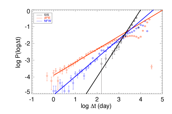
Figure 1: The logarithmic probability distribution of the time delays for three density profiles. They are the SIS profile (black), the dPIE density profile (red) and the NFW density profile (blue). The background sources are at $z=3$. The open circles and their poisson error bars are obtained from a numerical representation of the potentials. The best-fitting functions for each cluster are also plotted. The slopes of the best-fitting functions for the SIS profile, the NFW profile and the dPIE profile are $\beta_{\textrm{SIS}}=2.0$, $\beta_{\textrm{NFW}}=1.11$, $\beta_{\textrm{dPIE}}=0.78$.

To get the time-delay distribution, we create an input catalog of sources. Time delays are created when there are multiple images, so we need to make sure that the input source plane covers the area enclosed by the caustic line(s) and includes all potential multiply lensed sources. On the other hand, the input source plane should be sufficiently well sampled so as to be sensitive to the mass distribution and potential differences in the lens. This is to make sure that small time delays are also produced. In this work, we choose an input source plane covering an area of 60 $\times$ 60 arcsec with 200 $\times$ 200 pixels in the source plane at $z=3$. With the help of Lenstool [59], we can obtain a list of all images of every source in the source plane. Then we compute the differences in the arrival times between multiple images from each source. For example, for a source with 3 multiple images: image1, image2, image3, we compute the differences of arrival times between each two of these three images. Then we get 3 time delays in total.

3.1 The slope of the time-delay distribution

The time-delay distributions for the SIS, the NFW and the dPIE profiles are simulated and computed. In simulating the time-delay distributions, we choose parameters similar to those of mass models of real clusters. We adjust the parameters of the profiles to make their distributions overlap. The results are shown in figure 1. In the NFW mass model, the velocity dispersion is 1810 km/s, the concentration is 3.579 and the scale radius is 618 kpc. In the dPIE mass model, the velocity dispersion is 1500 km/s, the core radius is 72 kpc, and the cut radius is 2000 kpc. For the mass model described by the SIS profile, we set the velocity dispersion to 400 km/s. A change in the velocity dispersion will shift the distribution horizontally but keep the slope unchanged. So for computational convenience, we keep the velocity dispersion and shift the distribution horizontally to make the results for three profiles overlap. All three profiles are circular. With time delays less than 1000 days, the slopes of the logarithmic probability distribution functions for the SIS profile, the NFW profile and the dPIE profile, are $\beta_{\textrm{SIS}}=2.0$ as expected, $\beta_{\textrm{NFW}}=1.11$, $\beta_{\textrm{dPIE}}=0.78$, respectively (see also table 1). The difference in slopes of the distributions arises from the difference in the density slopes of the mass profiles, as discussed in section 2. This shows that the slope of the time-delay distribution is strongly affected by the mass distribution, especially the density slope of the cluster.

3.2 An example: Abell 1689

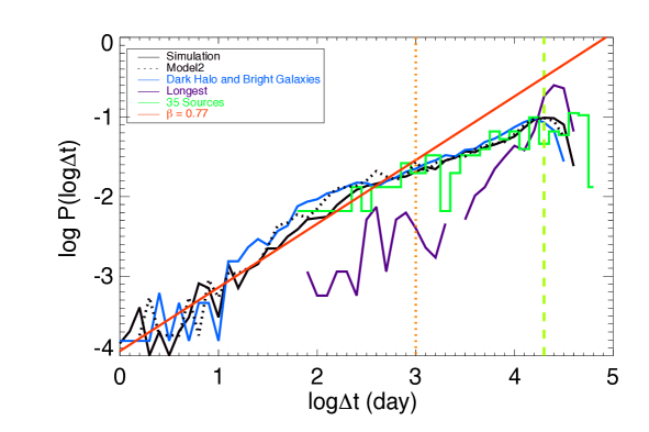
Figure 2: The time-delay distributions of Abell 1689 with modeled background sources at $z=3$. The time-delay distribution produced by the cluster with the full mass model is in black. The blue curve represents the time-delay distribution produced by the dark halo and a few bright galaxies (massive components), which fails to reproduce small time delays. The distribution of the selected longest time delays from each source is in purple. The red curve represents the logarithmic probability distribution function with $\beta=0.77$. The histogram in green represents the distribution of the time delays of 35 known multiply imaged sources. We are mainly interested in small time delays, i.e., those located to the left of the dotted orange line at 1000 days ($\log\Delta t$ = 3.0). The dashed line in olive represents $\Delta t_{\textrm{peak}}$.

With the help of deep Hubble Space Telescope (HST) imaging, Abell 1689 ($z=0.183$) displays a large number of multiple image systems at the center of the cluster. Using information from these systems, the mass model of Abell 1689 has been extensively studied. We base our work on the mass model consisting of 35 plausible lensed sources and 116 multiple images [60] [61] [7]. Among them, 25 sources have confirmed spectroscopic redshifts, the other 10 systems have lensing modeling redshifts or/and photometric redshifts.

To check how the time-delay distribution depends on the mass distribution, we split the mass model of Abell 1689 into two parts. The first part (massive components) consists of a dark halo and the three brightest galaxies with central velocity dispersions $\sigma\geqslant 500\,\textrm{km}\,\textrm{s}^{-1}$. The second part includes all other substructures (subcomponent), that is, all other gravitational potentials with velocity dispersions $\sigma$ smaller than $500\,\textrm{km}\,\textrm{s}^{-1}$. We compute the time-delay distribution in two different ways: First, we produce all time delays for Abell 1689 with the full mass model. Second, we compute time delays of Abell 1689 with only the mass model of the first part (massive components). The second part (subcomponent) itself produces only two multiple images, i.e., only one time delay. This is because most substructures do not gain enough mass to surpass the critical surface mass density, which is required for the structure to produce multiple images.

The time-delay distribution for Abell 1689 is shown in figure 2. The histogram in green represents the distribution of the time delays of the 35 known sources. It is consistent with the simulation of the grid of hypothetical sources. A logarithmic probability distribution function (2.13) with slope $\beta=0.77$ in red is also plotted. The blue curve represents the time delay distribution generated by the first part (massive components). From the figure, it is evident that the first part (massive components) succeeds in reproducing most relatively ‘large’ time delays, e.g., time delays larger than around 30 days. We conclude that small time delays are predominantly generated by substructures in the mass model.

The typical offset between the observed and modeled images is about $\sim$ 1^′′ [5]. Therefore, the individual time delays are affected. To test how the position offset affects the time-delay distribution, we plot the time delay distributions generated by two different mass models for Abell 1689. The result is shown in figure 2. The black curve represents the time-delay distribution applied in this paper, while the dotted curve is the result when another mass model [62] is used. Though different models may produce different time delays, the slope of the distribution of the time delays is not strongly affected.

The time-delay distribution of a real cluster may be more complicated than the ones discussed in section 2. The structure of the lensing cluster may consist of more clumps of potentials with more complicated mass distribution, thus each source may produce more than 2 multiple images. To check how these extra multiple images affect the time-delay distribution and whether the distributions for real clusters can also be fitted with the power-law functions, we also plot the distribution of the longest time delays generated by each source in figure 2. The figure shows firstly that compared to the ‘longest’ time delays, the total time-delay distribution can be fitted to a power-law function. Secondly, for small time delays, though none of them belong to the ‘longest’ time delays and there is no direct connection between the ansatz motivated by two image systems and those non-longest time delays, the distribution of the small time delays may also be fitted with a power-law function, which is implied by the simulation result of the total time delays. Finally, even though more multiple images are generated and more time delays are produced, the time-delay distribution still can be fitted well with a power-law function. Therefore, we proceed to apply the ansatz of the power-law functions (2.11) (2.12) deduced from two-image system to the real clusters with more multiple images.

4 Time delays in 17 clusters

4.1 Cluster selection and modeling

Cluster	$z$	RA (J2000.0)		Dec (J2000.0)		$M_{250}$	$\beta$
		[deg]		[deg]		($10^{14}\textrm{M}_{\odot}$)
Abell 2204	0.152	248.	195540	5.	575825	$2.29\pm 0.50$	$0.79\pm 0.03$
Abell 868	0.154	146.	359960	$-$8.	651994	$1.97\pm 1.11$	$0.57\pm 0.03$
RXJ 1720	0.164	260.	041860	26.	625627	$1.18\pm 0.59$	$0.64\pm 0.04$
Abell 2218	0.171	248.	954604	66.	212242	$3.00\pm 0.24$	$0.89\pm 0.04$
Abell 1689	0.183	197.	872954	$-$1.	341006	$4.53\pm 0.13$	$0.79\pm 0.03$
Abell 383	0.188	42.	014079	$-$3.	529040	$1.87\pm 0.26$	$0.85\pm 0.09$
Abell 773	0.217	139.	472660	51.	727024	$3.01\pm 0.58$	$0.86\pm 0.04$
RXJ 2129	0.235	322.	416510	0.	089227	$1.37\pm 0.37$	$0.74\pm 0.03$
Abell 1835	0.253	210.	258650	2.	878470	$2.83\pm 0.41$	$0.89\pm 0.05$
Abell 1703	0.280	198.	771971	51.	817494	$2.98\pm 0.09$	$0.77\pm 0.08$
MACS 2135	0.325	323.	800390	$-$1.	049624	$2.64\pm 0.04$	$0.83\pm 0.02$
MACS 1319	0.328	200.	034880	70.	077501	$2.28\pm 0.26$	$0.41\pm 0.06$
MACS 0712	0.328	108.	085460	59.	538994	$1.29\pm 0.27$	$0.63\pm 0.05$
MACS 0947	0.345	146.	803230	76.	387101	$2.96\pm 0.94$	$0.59\pm 0.09$
SMACS 2248	0.348	342.	183260	$-$44.	530966	$2.87\pm 0.06$	$0.80\pm 0.06$
MACS 1133	0.389	173.	304880	50.	144436	$1.52\pm 0.23$	$0.91\pm 0.05$
MACS 1347	0.451	206.	877570	$-$11.	752643	$3.86\pm 0.02$	$0.77\pm 0.05$

Table 2: Properties of 17 lensing clusters. The redshifts of the selected clusters range from 0.15 to 0.30 for models from LoCuSS and from 0.30 to 0.45 for MACS clusters. Here $M_{250}$ denotes the projected lensing mass inside 250 kpc [63] [62]. The slopes of $\beta$ in function (2.16) are also listed.

To further analyze the logarithmic probability distribution function of time delays and constrain the parameter and the constant in equation (2.13), we compute time-delay distributions by modeling 17 lensing clusters. The cluster selection procedure is based on two criteria: First, each lensing cluster system should have at least one image with a spectroscopically-confirmed redshift. Furthermore, the range of redshifts of the selected clusters should be as large as possible. The redshifts of the selected clusters range from 0.15 to 0.30 for models from LoCuSS [63] and from 0.30 to 0.45 for MACS models [62]. The selected clusters are listed in table 2.

The modeling procedure is the same as described in section 3. To make a reasonable comparison, the input source file for each cluster should have the same number of sources. Moreover, the whole source area should have the same size and be sufficiently sampled to cover the multiple image areas described by the caustic lines.

4.2 Estimating $\beta$

Figure 3: The distribution of parameter $\beta$ for probability distribution functions of 17 clusters. The modeling sources are at $z=3$. The probability distribution functions are fitted to the modeling data of time delays within 1000 days. The parameter range is $\beta\in[0.41,0.91]$.

.

As for Abell 1689 (section 3.2), we fit power-law distribution functions to time-delay distributions generated from the 17 cluster models. The functions are fitted to the data with time delays less than 1000 days. The cluster masses [61] [63] and the fitting values of $\beta$ are shown in table 2. The distribution of the parameter $\beta$ is shown in figure 3. The mean value is $\bar{\beta}=0.75$, and the median value is $\dot{\beta}=0.79$. With the least squares method, if the clusters are weighted equally to each other, we determine that the best-fitting slope is $\widetilde{\beta}=0.77$ for the 17 clusters, with standard deviations in $\log P(\Delta t)$ in the range [0.11, 0.30]. As a consequence, to a good approximation, $\beta$ can be fixed in equation (2.16).

4.3 Parameter estimation

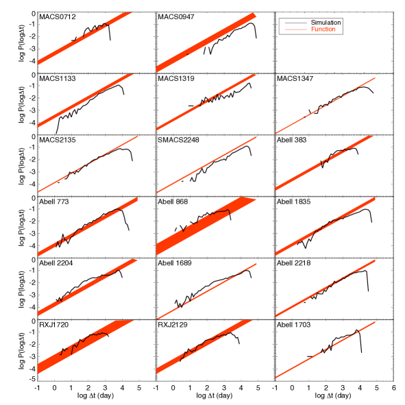
Figure 4: The logarithmic probability distribution functions for 17 clusters with background sources at $z=3$. The solid curves represent the modeling results of time-delay distribution of 17 clusters. The red shaded regions represent the logarithmic probability distribution function from equation (4.3). The uncertainties of the distribution functions arise from the uncertainties in the mass. For MACS1133, the input source area is 10 $\times$ 10 arcsec. For other clusters, the input source areas are 60 $\times$ 60 arcsec.

We fix the value of $\widetilde{\beta}=0.77$ in the logarithmic probability distribution function (2.16) and fit the function to the simulated data, and then find the best-fitting value for constant $C^{{}^{\prime}}_{2}$. With smallest deviations, we find that the best-fitting value is $C^{{}^{\prime}}_{2}=-3.28$. So the logarithmic probability distribution function (2.16) can be written as

$$\log P(\log\Delta t)=\widetilde{\beta}\log\Delta t-2\widetilde{\beta}\log M_{250}-3.28,$$ (4.1)

or

$$P(\log\Delta t)=5.27\times 10^{-4}\Delta t^{\widetilde{\beta}}/M_{250}^{2\widetilde{\beta}}.$$ (4.2)

If we introduce $\widetilde{\beta}=0.77$, then the logarithmic probability distribution function is simply

$$\log P(\log\Delta t)=0.77\log\Delta t-1.54\log M_{250}-3.28.$$ (4.3)

For a cluster with $M_{250}=2\times 10^{14}\ \textrm{M}_{\odot}$, the probability of a time delay less than 1000 days is about $0.025$. In figure 4, we present modeled time-delay distributions for all 17 clusters and their logarithmic probability distribution functions (4.3) with sources at $z=3$. Among the 17 systems, MACS1133 has much smaller multiple-image area enclosed by the caustic lines. To make the small time delays detectable, for MACS1133, we change the input source area to 10 $\times$ 10 arcsec. For other clusters, we keep the input source as 60 $\times$ 60 arcsec.

5 The rate of lensed supernovae in Abell 1689

With the help of the gravitational lensing amplification, we can potentially observe supernovae which would otherwise be too faint for detection. If a source is located inside the multiply imaged surface defined by the caustic line, two or more images will be generated. We may therefore observe multiple images of a supernova in the source galaxies.

For Abell 1689, we know 35 multiply imaged sources and 116 corresponding multiple images. For each multiple-image pair producing a time delay, we call the image arriving first to the observer the leading image. For example, for a source with 3 multiple images: image1, image2, image3, assuming the images have arrival times $\tau_{image1}<\tau_{image2}<\tau_{image3}$, there are three image pairs: $\textrm{pair}12$, $\textrm{pair}13$ and $\textrm{pair}23$. The corresponding leading images are $\textrm{image}1$, $\textrm{image}1$ and $\textrm{image}2$, accordingly. So in this three-image system, only the image with the longest arrival time (in this case, it is image3) cannot be the leading image. That is, for 1 source having 3 multiple images, the number of the leading images are $3-1=2$. Therefore, in a lensing system with $m$ sources and $n$ corresponding multiple images, the number of the leading images are $n-m$. According to this definition, in Abell 1689, there are $(116-35=)$ 81 leading images in total.

To estimate the probability of observing a leading supernovae image in Abell 1689, we need to know the supernova rate. The models for describing the supernova rate are dependent on the types of the supernova. The rate of core-collapse supernovae ($\textrm{SNR}_{\textrm{cc}}$) can be obtained from the star-formation rate:

$$\left(\frac{\textrm{SNR}_{\textrm{cc}}}{\textrm{yr}^{-1}}\right)=k_{\textrm{cc}}\cdot 10^{-3}\left(\frac{\textrm{SFR}}{\textrm{M}_{\odot}\ \textrm{yr}^{-1}}\right),$$ (5.1)

where the parameter $k_{\textrm{cc}}$ can be determined by measuring the $\textrm{SNR}_{\textrm{cc}}$ and SFR. Here the factor of $10^{-3}$ is multiplied into the function to simplify the parameter $k_{\textrm{cc}}$. We also multiply factors in the following functions (5.2) (5.7) for the same reason. The $\textrm{SNR}_{\textrm{cc}}$ and SFR can be derived from observational data [43] [64]. By using the core-collapse SN rate density and comparing it against the SFR density, the parameter is constrained to be $k_{\textrm{cc}}=7.5\pm 2.5$ [36]. Alternatively, by using a Salpeter IMF and a progenitor mass ranging between 8 and 50 solar masses, the parameter is estimated to be $k_{\textrm{cc}}=7$ [46]. In this paper, we choose $k_{\textrm{cc}}=10$ as the upper limit, and $k_{\textrm{cc}}=5$ as the lower limit.

For Type Ia supernovae, we use the popular “two-component”  model to estimate the Type Ia supernova rate ($\textrm{SNR}_{\textrm{Ia}}$) [36] [37] [38]:

$$\left(\frac{\textrm{SNR}_{\textrm{Ia}}}{\textrm{yr}^{-1}}\right)=\hat{A}\cdot 10^{-10}\left(\frac{M_{\star}}{\textrm{M}_{\odot}}\right)^{\alpha}+\hat{B}\cdot 10^{-3}\left(\frac{\textrm{SFR}}{\textrm{M}_{\odot}\textrm{yr}^{-1}}\right),$$ (5.2)

where $M_{\star}$ is the host stellar mass, and $\alpha$ denotes the exponent of the stellar mass. The first component describes the stellar mass contribution. The second component describes the host galaxy star-formation contribution. For parameters $\hat{A}$ and $\alpha$, we choose $\hat{A}=1.05\pm 0.16$ and $\alpha=0.68\pm 0.01$ [65]. The parameter $\hat{B}$ can be related to the $\textrm{SNR}_{\textrm{cc}}-\textrm{SFR}$ relation (5.1),

$$\hat{B}=k_{\textrm{cc}}\Theta,$$ (5.3)

where $\Theta=\textrm{SNR}_{\textrm{Ia}}/\textrm{SNR}_{\textrm{cc}}$. The value of $\Theta$ has been estimated at redshift up to $z\sim 1.5$ [43]. At redshift $z<1$, the ratio of $\textrm{SNR}_{\textrm{Ia}}/\textrm{SNR}_{\textrm{cc}}$ approximately ranges between $\Theta=1/2$ and $\Theta=1/4$, which is consistent with the result $\Theta=0.35\pm 0.08$ in nearby galaxies [37]. At higher redshift $z>1.0$, inspired from figure 3 of [43], we assume

$$\Theta=\frac{1}{15};\qquad 1.0\leq z.$$ (5.4)

Considering all sources in Abell 1689 have redshifts $z>1.0$, in this work, $\hat{B}=0.5\pm 0.17$. This value is consistent with $\hat{B}=0.39\pm 0.07$ (based on redshift $0.2<z<0.75$ [38]).

From their magnitude in F775W, we estimate the flux and the luminosity and then constrain their SFR [66] as

$$\left(\frac{\textrm{SFR}}{\textrm{M}_{\odot}\>\textrm{yr}^{-1}}\right)=1.4\times 10^{-28}\left(\frac{\bar{L}_{\nu}}{\textrm{erg}\,\textrm{ s}^{-1}\,\textrm{Hz}^{-1}}\right).$$ (5.5)

This conversion between UV flux and the SFR is for rest wavelengths, ranging from 1500 Å to 2800 Å, while our data [60] have observed wavelength in the range 6900 Å to 8600 Å. We assume these galaxies have flat spectra, as is typical for star-forming galaxies, so we can calculate the luminosity from the flux.

Figure 5: The cumulative rate ($N_{\textrm{SN}}$) of the leading images of lensed supernovae in Abell 1689, derived from equations (5.1) and (5.7). The magnitude threshold is 26.5 and a total number of 70 among the 72 leading images are included because of the magnitude threshold. The time delays are calculated based on the modeled source positions. The red curve represents the estimated cumulative $\textrm{SNR}_{\textrm{Ia}}$, while the cumulative $\textrm{SNR}_{\textrm{cc}}$ is plotted in blue curve. The uncertainties of $N_{\textrm{SN}}$ arise from the upper and lower limits of the parameters in the functions (5.1) (5.2) (5.7).

Note that multiple images from the same source should have the same inferred luminosity. To infer the luminosity of each image, we need to know their fluxes. With magnitudes of 116 images [60] [61], we can estimate their fluxes. Using Lenstool, we can get a magnification map on the image plane then read the values of the magnification on the map. Considering the gravitational magnification effect and k correction [67] [68], the flux can be calculated as

$$\log(F_{\nu})=[m_{\textrm{AB}}+2.5\log(|\mu|)+2.5\log(1+z)+48.6]/(-2.5),$$ (5.6)

where $\mu$ is the gravitational magnification factor, and $z$ is the source redshift. When images are located close to the caustics, their gravitational magnification factors ($\mu$) may be very large. Thus, the values of fluxes of these images derived from equation 5.6 are uncertain, and their luminosities estimated from the fluxes may not be reliable. So we neglect these images and average other luminosity values of images of the same source to constrain $\bar{L}_{\nu}$. When we know their luminosities, from equation (5.5), we can calculate their SFR, and then $\textrm{SNR}_{\textrm{Ia}}$ (5.7) and $\textrm{SNR}_{\textrm{cc}}$ (5.1).

We also need to calculate the stellar masses and the star-formation rates for each galaxy. To estimate the stellar-mass contribution to the SNR, we separate the images into two groups. In group one, with data of photometry from HST/ACS in bands B, V, I, Z, ground-based near-infrared imaging and Spitzer/IRAC photometry [61], we derive their stellar mass from SED fitting [69]. In group two with insufficient photometric data, we estimate the mass contribution based on the ratio of mass and star-formation contribution to the SNR derived from group one. The median value of this ratio, is only 2.9% (4.2%) of the upper (lower) limits of the star-formation part. In this paper, we choose its median value and assume the mass part contributes 3.5 % of the star-formation part. Therefore, for group two, the $\textrm{SNR}_{\textrm{Ia}}$ may be estimated as

$$\left(\frac{\textrm{SNR}_{\textrm{Ia}}}{\textrm{yr}^{-1}}\right)=1.035\cdot\hat{B}\cdot 10^{-3}\left(\frac{\textrm{SFR}}{\textrm{M}_{\odot}\textrm{yr}^{-1}}\right).$$ (5.7)

We assume Type Ia supernovae have absolute magnitude $M=-19.3$ mag [43], and core-collapse supernovae have $M=-17.0$ mag [70]. With their absolute magnitudes, considering the k correction, we calculate the apparent magnitudes for each supernova. Their apparent magnitudes of a supernova can be expressed as:

$$m=M+5\log_{10}(D_{L}/10\textrm{ pc})-2.5\log_{10}(|\mu|)-2.5\log_{10}(1+z).$$ (5.8)

Here $D_{L}$ denotes the luminosity distance. This equation is used to constrain the magnitude when considering the magnitude thresholds in figures 5 and 7.

The cumulative rate of observing the leading images of the lensed supernovae in Abell 1689 is shown in figure 5. Among the total 81 leading images, we exclude 14 images from 5 sources with insufficient magnitude data [60], so there are 72 leading images to be considered. Here $N_{\textrm{SN}}(<\log\Delta t)$ represents the cumulative rate of the supernova images observable in one year. We set the detection threshold to 26.5 mag in all bands. In that case, a total number of 70 of the 72 leading images are included. The resulting probabilities are $0.004\pm 0.002$ for the Type Ia supernovae and $0.029\pm 0.001$ for the core-collapse supernovae in one year, assuming time delays less than 1000 days.

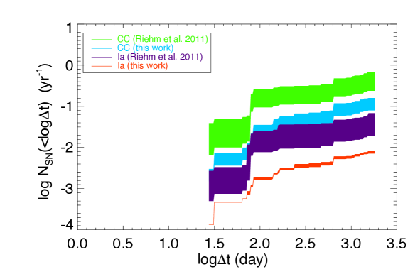
Figure 6: The comparison of the supernova rate estimated from functions (5.1) and (5.7), and the supernova rate from [46], with time delays less than 5 years. The green and purple curves represent the logarithmic cumulative $\textrm{SNR}_{\textrm{cc}}$ and $\textrm{SNR}_{\textrm{Ia}}$ from [46]. Our results are shown in blue for $\textrm{SNR}_{\textrm{cc}}$ and in red for $\textrm{SNR}_{\textrm{Ia}}$. The uncertainties of $\log N_{SN}$ arise from the upper and lower limits of the parameters in the functions (5.1) (5.2) (5.7). At $\log\Delta t\sim 1.8$, there is a fast increase in the $\log N_{\textrm{SN}}$. Firstly, in this region, there are more leading images included, so both our results and the results from [46] raise quickly. Secondly, the leading images have much larger SNR and uncertainties in their result. This causes an even faster raise and higher upper limit in their curves.

We also compare our results to the results from other groups [46]. The result is shown in figure 6. The difference in supernovae rates may arise from the difference in the lens model and/or the SNR prescription. For example, different lens models may produce different magnification factors for each images, and then produce different luminosities, and SFR. In addition, the different parameters chosen in the SNR model (5.2), e.g., $k_{\textrm{cc}}$, $\hat{A}$, $\alpha$, $\hat{B}$ may also affect the constraint on SNR. In this paper, we choose $k_{\textrm{cc}}=7.5\pm 2.5$, $\hat{A}=1.05\pm 0.16$, $\alpha=0.68\pm 0.01$, $\hat{B}=0.5\pm 0.17$, while in [46], the parameters are $k_{\textrm{cc}}=7.0$, $\hat{A}=4.4^{+1.6}_{-1.4}$, $\alpha=1.0$, $\hat{B}=2.6\pm 1.1$. Larger values of $\hat{A}$, $\alpha$, $\hat{B}$ chosen will cause a higher SNR estimate. We applied the parameters of [46] to the functions (5.1) (5.2) (5.7), in an attempt to reproduce their results. The results fit well to their $\textrm{SNR}_{\textrm{Ia}}$, but a significant discrepancies remain for $\textrm{SNR}_{\textrm{cc}}$.

We estimate the probability of observing the leading supernova images as a function of magnitude threshold in figure 7. The figure shows the cumulative rates of observable leading supernova images as a function of magnitude threshold, with time delays less than 1000 days. For a magnitude threshold of 27.0, we can observe $0.044\pm 0.015$ core-collapse supernovae per year, with time delays less than 1000 days. Under the conditions of small time-delay scales and limited magnitude threshold, the probability of observing a leading supernova image is quite low.

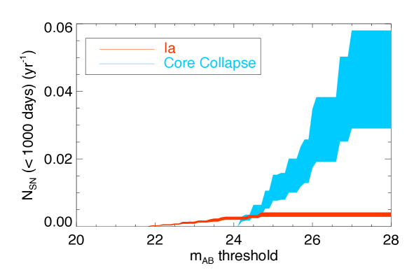
Figure 7: The cumulative rate of observing a leading supernovae image, as a function of magnitude threshold. The images have time-delay separations less than 1000 days. The uncertainties of $N_{\textrm{SN}}$ arise from the upper and lower limits of the parameters in the functions (5.1) (5.2) (5.7). The Type Ia supernovae involved are much brighter than those of the core-collapse supernovae. This causes a ‘shift’ in the distributions of the rates of Type Ia supernovae. At $m_{\textrm{AB}}$ around 24.7 for Type Ia supernovae, the curve flattens out. This is because all the Type Ia supernovae involved in the calculation have magnitudes smaller than about 24.7. The HST telescope has the magnitude limit in detecting the lensed sources. The James Webb Space Telescope may detect fainter lensed sources behind Abell 1689. As a sequence, Type Ia supernovae fainter than 24.7 will be detected, and the cumulative rate of observing a leading Type Ia supernovae ($N_{\textrm{SN}}$) will increase at $m_{\textrm{AB}}>24.7$ as well. This is also the case for the core-collapse supernovae when $m_{\textrm{AB}}>$ 27.0.

6 Summary and discussion

We analyzed the time-delay distributions in strong lensing systems. We found that we can describe the probability distribution of time delays as a power law function (2.16). In the function, there are two parameters, $M_{250}$, $\beta$, and a constant $C^{{}^{\prime}}_{2}$. Modeling with mass profiles of SIS, NFW and dPIE (in figure 1), we found that the parameter $\beta$ is strongly affected by the slopes of the mass profiles of the lensing clusters. The shallower the inner density profile and the steeper the outer density profile are, the more the time-delay distribution will be stretched out to both the higher and the lower end, causing a lower $\beta$. By modeling Abell 1689, we found that the massive galaxies and halos mainly produce large time delays, while small time delays are predominated produced by substructures (galaxies) in the cluster. We also simulated and verified that the time-delay distribution generated by ‘real’ clusters with more than 2 multiple images from the same sources also obey the power-law distribution in figure 2.

To estimate the parameter and the constant in the logarithmic probability distribution function, we modeled 17 strong lensing clusters as shown in figure 4, using their well calibrated mass models. With the fixed best-fitting slope $\widetilde{\beta}=0.77$, we determined the best-fitting value of $C^{{}^{\prime}}_{2}$ to the function (2.16). The resultant logarithmic probability distribution function (4.3) enables us to estimate the time-delay distribution of a cluster with known mass.

We also calculated the probability of observing the leading images of the lensed supernovae in Abell 1689. The $\textrm{SNR}_{\textrm{cc}}$ can be derived from the SFR (5.1). The “two component”  model was applied to constrain the $\textrm{SNR}_{\textrm{Ia}}$. We constrained the parameters in the function (5.2), and calculated the SNR for Type Ia supernova. We estimated the luminosity from magnitudes of images in Abell 1689 (5.6), derived the SFR from the luminosity (5.5), and then estimated the probability of observing a leading supernova image in the system as shown in figure 5. Considering a typical magnitude limit of observations with $m_{\textrm{AB}}=26.5$, we can observe $0.004\pm 0.002$ Type Ia supernovae and $0.029\pm 0.001$ core-collapse supernovae per year. We compared the results in this work to [46] as shown in figure 6, and discussed the possible reasons which may cause the differences.

We also constrained the cumulative rate of observing a leading supernovae image, as a function of the magnitude threshold (in figure 7). If the magnitude limit is lowered to 27.0, the probability of observing the leading images of the core-collapse supernovae will be up to $0.044\pm 0.015$ per year, with image separations within 1000 days. This probability is quite low, which means that detecting time delays from lensed supernovae will be challenging with current facilities.

References

- [1] F. Zwicky, On the Probability of Detecting Nebulae Which Act as Gravitational Lenses, Physical Review 51 (Apr., 1937) 679–679.
- [2] J. H. Cooke and R. Kantowski, Time Delay for Multiply Imaged Quasars, Astrophys. J. Lett. 195 (Jan., 1975) L11+.
- [3] R. D. Blandford and R. Narayan, Cosmological applications of gravitational lensing, Annual Review of Astronomy and Astrophysics 30 (1992) 311–358.
- [4] G. Efstathiou, W. J. Sutherland, and S. J. Maddox, The cosmological constant and cold dark matter, Nature 348 (Dec., 1990) 705–707.
- [5] J.-P. Kneib and P. Natarajan, Cluster lenses, The Astronomy and Astrophysics Review 19 (Nov., 2011) 47, [arXiv:1202.0185].
- [6] S. Refsdal, On the possibility of determining Hubble’s parameter and the masses of galaxies from the gravitational lens effect, Mon. Not. R. Astron. Soc. 128 (1964) 307–+.
- [7] E. Jullo, P. Natarajan, J.-P. Kneib, A. D’Aloisio, M. Limousin, J. Richard, and C. Schimd, Cosmological Constraints from Strong Gravitational Lensing in Clusters of Galaxies, Science 329 (Aug., 2010) 924–927, [arXiv:1008.4802].
- [8] C. S. Kochanek and P. L. Schechter, The Hubble Constant from Gravitational Lens Time Delays, Measuring and Modeling the Universe (2004) 117–+, [astro-ph/0306040].
- [9] R. Massey, T. Kitching, and J. Richard, The dark matter of gravitational lensing, Reports on Progress in Physics 73 (Aug., 2010) 086901–+, [arXiv:1001.1739].
- [10] P. Schneider, J. Ehlers, and E. Falco, Gravitational Lenses. Springer-Verlag, 1992.
- [11] P. Saha, J. Coles, A. V. Macciò, and L. L. R. Williams, The Hubble Time Inferred from 10 Time Delay Lenses, Astrophys. J. Lett. 650 (Oct., 2006) L17–L20, [astro-ph/0607240].
- [12] D. Paraficz and J. Hjorth, The Hubble Constant Inferred from 18 Time-delay Lenses, Astrophys. J. 712 (Apr., 2010) 1378–1384, [arXiv:1002.2570].
- [13] S. H. Suyu, M. W. Auger, S. Hilbert, P. J. Marshall, M. Tewes, T. Treu, C. D. Fassnacht, L. V. E. Koopmans, D. Sluse, R. D. Blandford, F. Courbin, and G. Meylan, Two accurate time-delay distances from strong lensing: Implications for cosmology, ArXiv e-prints (Aug., 2012) [arXiv:1208.6010].
- [14] D. Rusin, Constraining Galaxy Mass Profiles with Strong Gravitational Lensing, ArXiv Astrophysics e-prints (Apr., 2000) [astro-ph/0004241].
- [15] D. Paraficz and J. Hjorth, Gravitational lenses as cosmic rulers: , from time delays and velocity dispersions, Astron. Astrophys. 507 (2009) 49–52, [arXiv:0910.5823].
- [16] D. Coe and L. A. Moustakas, Cosmological Constraints from Gravitational Lens Time Delays, Astrophys. J. 706 (Nov., 2009) 45–59, [arXiv:0906.4108].
- [17] S. H. Suyu, P. J. Marshall, M. W. Auger, S. Hilbert, R. D. Blandford, L. V. E. Koopmans, C. D. Fassnacht, and T. Treu, Dissecting the Gravitational lens B1608+656. II. Precision Measurements of the Hubble Constant, Spatial Curvature, and the Dark Energy Equation of State, Astrophys. J. 711 (Mar., 2010) 201–221, [arXiv:0910.2773].
- [18] E. V. Linder, Lensing time delays and cosmological complementarity, Phys. Rev. D 84 (Dec., 2011) 123529, [arXiv:1109.2592].
- [19] L. J. Goicoechea and V. N. Shalyapin, Time Delays in the Gravitationally Lensed Quasar H1413+117 (Cloverleaf), ApJ 708 (Jan., 2010) 995–1001, [arXiv:0911.4829].
- [20] M. Hamuy, M. M. Phillips, N. B. Suntzeff, R. A. Schommer, J. Maza, A. R. Antezan, M. Wischnjewsky, G. Valladares, C. Muena, L. E. Gonzales, R. Aviles, L. A. Wells, R. C. Smith, M. Navarrete, R. Covarrubias, G. M. Williger, A. R. Walker, A. C. Layden, J. H. Elias, J. A. Baldwin, M. Hernandez, H. Tirado, P. Ugarte, R. Elston, N. Saavedra, F. Barrientos, E. Costa, P. Lira, M. T. Ruiz, C. Anguita, X. Gomez, P. Ortiz, M. della Valle, J. Danziger, J. Storm, Y.-C. Kim, C. Bailyn, E. P. Rubenstein, D. Tucker, S. Cersosimo, R. A. Mendez, L. Siciliano, W. Sherry, B. Chaboyer, R. A. Koopmann, D. Geisler, A. Sarajedini, A. Dey, N. Tyson, R. M. Rich, R. Gal, R. Lamontagne, N. Caldwell, P. Guhathakurta, A. C. Phillips, P. Szkody, C. Prosser, L. C. Ho, R. McMahan, G. Baggley, K.-P. Cheng, R. Havlen, K. Wakamatsu, K. Janes, M. Malkan, F. Baganoff, P. Seitzer, M. Shara, C. Sturch, J. Hesser, A. N. P. Hartig, J. Hughes, D. Welch, T. B. Williams, H. Ferguson, P. J. Francis, L. French, M. Bolte, J. Roth, S. Odewahn, S. Howell, and W. Krzeminski, BVRI Light Curves for 29 Type IA Supernovae, Astron. J. 112 (Dec., 1996) 2408, [astro-ph/9609064].
- [21] W. Hillebrandt and J. C. Niemeyer, Type IA Supernova Explosion Models, Annual Review of Astronomy and Astrophysics 38 (2000) 191–230, [astro-ph/0006305].
- [22] M. Oguri and Y. Kawano, Gravitational lens time delays for distant supernovae: breaking the degeneracy between radial mass profiles and the Hubble constant, Mon. Not. R. Astron. Soc. 338 (Feb., 2003) L25–L29, [astro-ph/0211499].
- [23] A. G. Riess, A. V. Filippenko, P. Challis, A. Clocchiatti, A. Diercks, P. M. Garnavich, R. L. Gilliland, C. J. Hogan, S. Jha, R. P. Kirshner, B. Leibundgut, M. M. Phillips, D. Reiss, B. P. Schmidt, R. A. Schommer, R. C. Smith, J. Spyromilio, C. Stubbs, N. B. Suntzeff, and J. Tonry, Observational Evidence from Supernovae for an Accelerating Universe and a Cosmological Constant, Astron. J. 116 (Sept., 1998) 1009–1038, [astro-ph/9805201].
- [24] S. Perlmutter, G. Aldering, G. Goldhaber, R. A. Knop, P. Nugent, P. G. Castro, S. Deustua, S. Fabbro, A. Goobar, D. E. Groom, I. M. Hook, A. G. Kim, M. Y. Kim, J. C. Lee, N. J. Nunes, R. Pain, C. R. Pennypacker, R. Quimby, C. Lidman, R. S. Ellis, M. Irwin, R. G. McMahon, P. Ruiz-Lapuente, N. Walton, B. Schaefer, B. J. Boyle, A. V. Filippenko, T. Matheson, A. S. Fruchter, N. Panagia, H. J. M. Newberg, W. J. Couch, and The Supernova Cosmology Project, Measurements of Omega and Lambda from 42 High-Redshift Supernovae, Astrophys. J. 517 (June, 1999) 565–586, [astro-ph/9812133].
- [25] J. Nordin, L. Östman, A. Goobar, R. Amanullah, R. C. Nichol, M. Smith, J. Sollerman, B. A. Bassett, J. Frieman, P. M. Garnavich, G. Leloudas, M. Sako, and D. P. Schneider, Spectral properties of type Ia supernovae up to z 0.3, Astron. Astrophys. 526 (Feb., 2011) A119+, [arXiv:1011.6227].
- [26] C. Gall, J. Hjorth, and A. C. Andersen, Production of dust by massive stars at high redshift, The Astronomy and Astrophysics Review 19 (Sept., 2011) 43, [arXiv:1108.0403].
- [27] D. Maoz and F. Mannucci, Type-Ia supernova rates and the progenitor problem, a review, ArXiv e-prints (Nov., 2011) [arXiv:1111.4492].
- [28] J. Whelan and I. Iben, Jr., Binaries and Supernovae of Type I, Astrophys. J. 186 (Dec., 1973) 1007–1014.
- [29] F. Hoyle and W. A. Fowler, Nucleosynthesis in Supernovae., Astrophys. J. 132 (Nov., 1960) 565+–.
- [30] D. Branch, M. Livio, L. R. Yungelson, F. R. Boffi, and E. Baron, In Search of the Progenitors of Type Ia Supernovae, Publications of the Astronomical Society of the Pacific 107 (Nov., 1995) 1019–+.
- [31] R. F. Webbink, Double white dwarfs as progenitors of R Coronae Borealis stars and Type I supernovae, Astrophys. J. 277 (Feb., 1984) 355–360.
- [32] M. Fink, W. Hillebrandt, and F. K. Röpke, Double-detonation supernovae of sub-Chandrasekhar mass white dwarfs, Astron. Astrophys. 476 (Dec., 2007) 1133–1143, [arXiv:0710.5486].
- [33] L. Bildsten, K. J. Shen, N. N. Weinberg, and G. Nelemans, Faint Thermonuclear Supernovae from AM Canum Venaticorum Binaries, Astrophys. J. Lett. 662 (June, 2007) L95–L98, [astro-ph/0703578].
- [34] J. Guillochon, M. Dan, E. Ramirez-Ruiz, and S. Rosswog, Surface Detonations in Double Degenerate Binary Systems Triggered by Accretion Stream Instabilities, Astrophys. J. Lett. 709 (Jan., 2010) L64–L69, [arXiv:0911.0416].
- [35] J. P. Anderson, S. M. Habergham, and P. A. James, On the multiple supernova population of Arp 299: constraints on progenitor properties and host galaxy star formation characteristics, Mon. Not. R. Astron. Soc. 416 (Sept., 2011) 567–579, [arXiv:1105.2837].
- [36] E. Scannapieco and L. Bildsten, The Type Ia Supernova Rate, Astrophys. J. Lett. 629 (Aug., 2005) L85–L88, [astro-ph/0507456].
- [37] F. Mannucci, M. Della Valle, N. Panagia, E. Cappellaro, G. Cresci, R. Maiolino, A. Petrosian, and M. Turatto, The supernova rate per unit mass, Astron. Astrophys. 433 (Apr., 2005) 807–814, [astro-ph/0411450].
- [38] M. Sullivan, D. Le Borgne, C. J. Pritchet, A. Hodsman, J. D. Neill, D. A. Howell, R. G. Carlberg, P. Astier, E. Aubourg, D. Balam, S. Basa, A. Conley, S. Fabbro, D. Fouchez, J. Guy, I. Hook, R. Pain, N. Palanque-Delabrouille, K. Perrett, N. Regnault, J. Rich, R. Taillet, S. Baumont, J. Bronder, R. S. Ellis, M. Filiol, V. Lusset, S. Perlmutter, P. Ripoche, and C. Tao, Rates and Properties of Type Ia Supernovae as a Function of Mass and Star Formation in Their Host Galaxies, Astrophys. J. 648 (Sept., 2006) 868–883, [astro-ph/0605455].
- [39] B. Dilday, R. Kessler, J. A. Frieman, J. Holtzman, J. Marriner, G. Miknaitis, R. C. Nichol, R. Romani, M. Sako, B. Bassett, A. Becker, D. Cinabro, F. DeJongh, D. L. Depoy, M. Doi, P. M. Garnavich, C. J. Hogan, S. Jha, K. Konishi, H. Lampeitl, J. L. Marshall, D. McGinnis, J. L. Prieto, A. G. Riess, M. W. Richmond, D. P. Schneider, M. Smith, N. Takanashi, K. Tokita, K. van der Heyden, N. Yasuda, C. Zheng, J. Barentine, H. Brewington, C. Choi, A. Crotts, J. Dembicky, M. Harvanek, M. Im, W. Ketzeback, S. J. Kleinman, J. Krzesiński, D. C. Long, E. Malanushenko, V. Malanushenko, R. J. McMillan, A. Nitta, K. Pan, G. Saurage, S. A. Snedden, S. Watters, J. C. Wheeler, and D. York, A Measurement of the Rate of Type Ia Supernovae at Redshift 0.1 from the First Season of the SDSS-II Supernova Survey, Astrophys. J. 682 (July, 2008) 262–282, [arXiv:0801.3297].
- [40] B. Dilday, M. Smith, B. Bassett, A. Becker, R. Bender, F. Castander, D. Cinabro, A. V. Filippenko, J. A. Frieman, L. Galbany, P. M. Garnavich, A. Goobar, U. Hopp, Y. Ihara, S. W. Jha, R. Kessler, H. Lampeitl, J. Marriner, R. Miquel, M. Mollá, R. C. Nichol, J. Nordin, A. G. Riess, M. Sako, D. P. Schneider, J. Sollerman, J. C. Wheeler, L. Östman, D. Bizyaev, H. Brewington, E. Malanushenko, V. Malanushenko, D. Oravetz, K. Pan, A. Simmons, and S. Snedden, Measurements of the Rate of Type Ia Supernovae at Redshift 0.3 from the Sloan Digital Sky Survey II Supernova Survey, Astrophys. J. 713 (Apr., 2010) 1026–1036, [arXiv:1001.4995].
- [41] J. D. Neill, M. Sullivan, D. Balam, C. J. Pritchet, D. A. Howell, K. Perrett, P. Astier, E. Aubourg, S. Basa, R. G. Carlberg, A. Conley, S. Fabbro, D. Fouchez, J. Guy, I. Hook, R. Pain, N. Palanque-Delabrouille, N. Regnault, J. Rich, R. Taillet, G. Aldering, P. Antilogus, V. Arsenijevic, C. Balland, S. Baumont, J. Bronder, R. S. Ellis, M. Filiol, A. C. Gonçalves, D. Hardin, M. Kowalski, C. Lidman, V. Lusset, M. Mouchet, A. Mourao, S. Perlmutter, P. Ripoche, D. Schlegel, and C. Tao, The Type Ia Supernova Rate at z 0.5 from the Supernova Legacy Survey, Astron. J. 132 (Sept., 2006) 1126–1145, [astro-ph/0605148].
- [42] K. Perrett, M. Sullivan, A. Conley, S. González-Gaitán, R. Carlberg, D. Fouchez, P. Ripoche, J. D. Neill, P. Astier, D. Balam, C. Balland, S. Basa, J. Guy, D. Hardin, I. M. Hook, D. A. Howell, R. Pain, N. Palanque-Delabrouille, C. Pritchet, N. Regnault, J. Rich, V. Ruhlmann-Kleider, S. Baumont, C. Lidman, S. Perlmutter, and E. S. Walker, Evolution in the Volumetric Type Ia Supernova Rate from the Supernova Legacy Survey, Astron. J. 144 (Aug., 2012) 59, [arXiv:1206.0665].
- [43] T. Dahlen, L.-G. Strolger, A. G. Riess, B. Mobasher, R.-R. Chary, C. J. Conselice, H. C. Ferguson, A. S. Fruchter, M. Giavalisco, M. Livio, P. Madau, N. Panagia, and J. L. Tonry, High-Redshift Supernova Rates, Astrophys. J. 613 (Sept., 2004) 189–199, [astro-ph/0406547].
- [44] T. Dahlen, L.-G. Strolger, and A. G. Riess, The Extended HST Supernova Survey: The Rate of SNe Ia at z 1.4 Remains Low, Astrophys. J. 681 (July, 2008) 462–469, [arXiv:0803.1130].
- [45] O. Graur, D. Poznanski, D. Maoz, N. Yasuda, T. Totani, M. Fukugita, A. V. Filippenko, R. J. Foley, J. M. Silverman, A. Gal-Yam, A. Horesh, and B. T. Jannuzi, Supernovae in the Subaru Deep Field: the rate and delay-time distribution of type Ia supernovae out to redshift 2, ArXiv e-prints (Jan., 2011) [arXiv:1102.0005].
- [46] T. Riehm, E. Mörtsell, A. Goobar, R. Amanullah, T. Dahlén, J. Jönsson, M. Limousin, K. Paech, and J. Richard, Near-IR search for lensed supernovae behind galaxy clusters. III. Implications for cluster modeling and cosmology, Astron. Astrophys. 536 (Dec., 2011) A94, [arXiv:1109.6351].
- [47] R. Narayan and M. Bartelmann, Lectures on Gravitational Lensing, ArXiv Astrophysics e-prints (June, 1996) [astro-ph/9606001].
- [48] H. J. Witt, S. Mao, and C. R. Keeton, Analytic Time Delays and H0 Estimates for Gravitational Lenses, Astrophys. J. 544 (Nov., 2000) 98–103, [astro-ph/0004069].
- [49] C. R. Keeton, C. S. Kochanek, and U. Seljak, Shear and Ellipticity in Gravitational Lenses, Astrophys. J. 482 (June, 1997) 604, [astro-ph/9610163].
- [50] H. J. Witt and S. Mao, Probing the structure of lensing galaxies with quadruple lenses: the effect of ‘external’ shear, Mon. Not. R. Astron. Soc. 291 (Oct., 1997) 211–218, [astro-ph/9702021].
- [51] C. S. Kochanek, What Do Gravitational Lens Time Delays Measure?, Astrophys. J. 578 (Oct., 2002) 25–32, [astro-ph/0205319].
- [52] M. Oguri, A. Taruya, Y. Suto, and E. L. Turner, Strong Gravitational Lensing Time Delay Statistics and the Density Profile of Dark Halos, Astrophys. J. Lett. 568 (Apr., 2002) 488–499, [astro-ph/0112119].
- [53] J. Samsing, private communication, .
- [54] C. R. Keeton and P. Madau, Lensing Constraints on the Cores of Massive Dark Matter Halos, Astrophys. J. Lett. 549 (Mar., 2001) L25–L28, [astro-ph/0101058].
- [55] J. S. B. Wyithe, E. L. Turner, and D. N. Spergel, Gravitational Lens Statistics for Generalized NFW Profiles: Parameter Degeneracy and Implications for Self-Interacting Cold Dark Matter, Astrophys. J. 555 (July, 2001) 504–523, [astro-ph/0007354].
- [56] Á. Elíasdóttir, M. Limousin, J. Richard, J. Hjorth, J.-P. Kneib, P. Natarajan, K. Pedersen, E. Jullo, and D. Paraficz, Where is the matter in the Merging Cluster Abell 2218?, ArXiv e-prints (Oct., 2007) [arXiv:0710.5636].
- [57] J. F. Navarro, C. S. Frenk, and S. D. M. White, The Structure of Cold Dark Matter Halos, Astrophys. J. 462 (May, 1996) 563–+, [astro-ph/9508025].
- [58] J. Binney and S. Tremaine, GALACTIC DYNAMICS. Princeton Series in Astrophysics.
- [59] E. Jullo, J.-P. Kneib, M. Limousin, Á. Elíasdóttir, P. J. Marshall, and T. Verdugo, A Bayesian approach to strong lensing modelling of galaxy clusters, New Journal of Physics 9 (Dec., 2007) 447–+, [arXiv:0706.0048].
- [60] M. Limousin, J. Richard, E. Jullo, J.-P. Kneib, B. Fort, G. Soucail, Á. Elíasdóttir, P. Natarajan, R. S. Ellis, I. Smail, O. Czoske, G. P. Smith, P. Hudelot, S. Bardeau, H. Ebeling, E. Egami, and K. K. Knudsen, Combining Strong and Weak Gravitational Lensing in Abell 1689, The Astrophysical Journal 668 (Oct., 2007) 643–666, [astro-ph/0612165].
- [61] J. Richard, paper in preparation, .
- [62] J. Richard, private communication, .
- [63] J. Richard, G. P. Smith, J.-P. Kneib, R. S. Ellis, A. J. R. Sanderson, L. Pei, T. A. Targett, D. J. Sand, A. M. Swinbank, H. Dannerbauer, P. Mazzotta, M. Limousin, E. Egami, E. Jullo, V. Hamilton-Morris, and S. M. Moran, LoCuSS: first results from strong-lensing analysis of 20 massive galaxy clusters at z = 0.2, Mon. Not. R. Astron. Soc. 404 (May, 2010) 325–349, [arXiv:0911.3302].
- [64] M. Giavalisco, M. Dickinson, H. C. Ferguson, S. Ravindranath, C. Kretchmer, L. A. Moustakas, P. Madau, S. M. Fall, J. P. Gardner, M. Livio, C. Papovich, A. Renzini, H. Spinrad, D. Stern, and A. Riess, The Rest-Frame Ultraviolet Luminosity Density of Star-forming Galaxies at Redshifts z 3.5, Astrophys. J. Lett. 600 (Jan., 2004) L103–L106, [astro-ph/0309065].
- [65] M. Smith, R. C. Nichol, B. Dilday, J. Marriner, R. Kessler, B. Bassett, D. Cinabro, J. Frieman, P. Garnavich, S. W. Jha, H. Lampeitl, M. Sako, D. P. Schneider, and J. Sollerman, The SDSS-II Supernova Survey: Parameterizing the Type Ia Supernova Rate as a Function of Host Galaxy Properties, ArXiv e-prints (Aug., 2011) [arXiv:1108.4923].
- [66] R. C. Kennicutt, Jr., Star Formation in Galaxies Along the Hubble Sequence, Ann.Rev.Astron.Astrophys 36 (1998) 189–232, [astro-ph/9807187].
- [67] D. W. Hogg, I. K. Baldry, M. R. Blanton, and D. J. Eisenstein, The K correction, ArXiv Astrophysics e-prints (Oct., 2002) [astro-ph/0210394].
- [68] P. G. van Dokkum and M. Franx, The Fundamental Plane in CL 0024 at z = 0.4: implications for the evolution of the mass-to-light ratio., Mon. Not. R. Astron. Soc 281 (Aug., 1996) 985–1000, [astro-ph/9603063].
- [69] J. Walcher, B. Groves, T. Budavári, and D. Dale, Fitting the integrated spectral energy distributions of galaxies, Astrophysics and Space Science 331 (Jan., 2011) 1–52, [arXiv:1008.0395].
- [70] C. B. D’Andrea, M. Sako, B. Dilday, J. A. Frieman, J. Holtzman, R. Kessler, K. Konishi, D. P. Schneider, J. Sollerman, J. C. Wheeler, N. Yasuda, D. Cinabro, S. Jha, R. C. Nichol, H. Lampeitl, M. Smith, D. W. Atlee, B. Bassett, F. J. Castander, A. Goobar, R. Miquel, J. Nordin, L. Östman, J. L. Prieto, R. Quimby, A. G. Riess, and M. Stritzinger, Type II-P Supernovae from the SDSS-II Supernova Survey and the Standardized Candle Method, Astrophys. J. 708 (Jan., 2010) 661–674, [arXiv:0910.5597].