Radiation thermo-chemical models of protoplanetary discs

Abstract

Context. The carbon monoxide (CO) ro-vibrational emission from discs around Herbig Ae stars and T Tauri stars with strong ultraviolet emissions suggests that fluorescence pumping from the ground $X^{1}\Sigma^{+}$ to the electronic $A^{1}\Pi$ state of CO should be taken into account in disc models.

Aims. We wish to understand the excitation mechanism of CO ro-vibrational emission seen in Herbig Ae discs, in particular in transitions involving highly excited rotational and vibrational levels.

Methods. We implemented a CO model molecule that includes up to 50 rotational levels within nine vibrational levels for the ground and $A$-excited states in the radiative-photochemical code ProDiMo. We took CO collisions with hydrogen molecules (H₂), hydrogen atoms (H), helium (He), and electrons into account. We estimated the missing collision rates using standard scaling laws and discussed their limitations. We tested the effectiveness of UV fluorescence pumping for the population of high-vibrational levels ($v$=1–9, $J$=1–50) for four Herbig Ae disc models (disc mass $M_{\mathrm{disc}}$=10^-2, 10^-4 and inner radius $R_{\mathrm{disc}}$=1, 20 AU). We tested the effect of infrared (IR) pumping on the CO vibrational temperature and the rotational population in the ground vibrational level.

Results. UV fluorescence and IR pumping impact on the population of ro-vibrational $v>1$ levels. The $v=1$ rotational levels are populated at rotational temperatures between the radiation temperature around 4.6 $\mu$m and the gas kinetic temperature. The UV pumping efficiency increases with decreasing disc mass. The consequence is that the vibrational temperatures $T_{\mathrm{vib}}$, which measure the relative populations between the vibrational levels, are higher than the disc gas kinetic temperatures (suprathermal population of the vibrational levels). The effect is more important for low-density gases because of lower collisional de-excitations.The UV pumping is more efficient for low-mass ($M_{\mathrm{disc}}<$ 10^-3 M_⊙) than high-mass ($M_{\mathrm{disc}}>$ 10^-3 M_⊙) discs. Rotational temperatures from fundamental transitions derived using optically thick ¹²CO $v=1-0$ lines do not reflect the gas kinetic temperature. Uncertainties in the rate coefficients within an order of magnitude result in variations in the CO line fluxes up to 20%. CO pure rotational levels with energies lower than 1000 K are populated in LTE but are sensitive to a number of vibrational levels included in the model. The ¹²CO pure rotational lines are highly optically thick for transition from levels up to $E_{\mathrm{upper}}$=2000 K. The model line fluxes are comparable with the observed line fluxes from typical HerbigAe low- and high-mass discs.

1 Introduction

Terrestrial planets form in the inner region of protoplanetary discs (typically $R<$3-5 AU), where the gas reaches temperatures of a few hundred to a few thousand degrees Kelvin and the dust grains are warm enough such that water is not frozen onto their surfaces (Kamp et al. 2010). The growth of solid cores in the inner disc is slower than in the outer disc, where grains are coated with an icy mantle. As a consequence, the solid bodies never reach the critical mass to attract gravitationally the disc gas before the gas disc has dissipated (Armitage 2010).

At a few hundred to a few thousand degrees, molecules are excited to their ro-vibrational levels and emit in the near- and mid-infrared. Probing the warm gas emissions requires high angular-resolution observations in the infrared. Carbon monoxide is one of the most abundant species in protoplanetary discs, and its ro-vibrational transitions around 4.6 micron ($M$-band) are the most commonly detected lines with high spectral resolution adaptive-optics (AO) assisted spectrometers around T Tauri (Najita et al. 2003; Rettig et al. 2004; Salyk et al. 2011) and Herbig Ae stars (Blake & Boogert 2004; Carmona et al. 2005; Brittain et al. 2009; van der Plas et al. 2009). The CO peak emission is also seen displaced from the source centre, suggesting the presence of an inner hole (Brittain et al. 2003; Goto et al. 2006; Brown et al. 2012). The spectro-astrometric technique further improves our understanding of the emission by reaching spatial resolutions of the order of 0.1–0.5 AU for nearby (100-140 pc) discs (Pontoppidan et al. 2008). Goto et al. (2012) observed the CO ro-vibrational emission from the HD~100546 disc with a spatial resolution of 10 AU at 100 pc. They found warm CO gas (400-500) out to a distance of 50 AU, which is evidence for the presence of a warm molecular disc atmosphere. Very dense and hot gas located within a few tenths of AU from the stars can be detected by the CO overtone emissions (Tatulli et al. 2008; Berthoud et al. 2007; Thi et al. 2005).

Line profiles are diverse, from broad single peaked to clear double peaked; the latter is a signature of Keplerian rotation of the gas between 1 and 5 AU (Salyk et al. 2009). Bast et al. (2011) focused on 8 out of 50 discs that show broad single-peaked CO profiles. They proposed that those 8 discs have either highly turbulent inner disc gas and/or that a slowly moving disc wind contributes to the emission.

The $M$-band observations show lines emitted from a large range of excitation levels (from fundamental $v=1\rightarrow 0$ $P$(1) and $R$(0) lines to “hot” lines ($v^{\prime}>1$, $\Delta v=1$) which make it possible to probe disc regions with different excitation conditions. CO vibrational diagrams of Herbig Ae discs indicate vibrational gas temperatures higher than the rotational ones (a few thousand K instead of a few hundred K). This suggests that the population of high vibrational levels ($v>$1) may be dominated by IR and UV fluorescence excitation (Brittain et al. 2007; Brown et al. 2012). The $v>$ 1 ro-vibrational levels can also be efficiently populated by UV fluorescence for T Tauri discs, especially for strongly accreting systems with excess UV emission (Bast et al. 2011). Fluorescence excitation in T Tauri discs is supported by Hubble Space Telescope observations of UV-pumped CO emission (France et al. 2011).

Many models of CO ro-vibrational emission made the assumption of local thermodynamical equilibrium (LTE) population (Hügelmeyer et al. 2009; Regály et al. 2010; Salyk et al. 2011). Nevertheless, a detailed understanding of the CO ro-vibrational lines, especially the spatial location of the lines and the efficiency of the IR/UV fluorescence, requires non local thermodynamic equilibrium (NLTE) modelling and a chemo-physical code that includes detailed continuum and line radiative transfer. The accuracy of NLTE modelling depends on many factors, including the availability of accurate collision rates. The difficulties associated with the measurement and computation of accurate rates result in sparse trustworthy data. Completeness in the rate coefficients can be attained only by using approximate extrapolation rules derived from physical considerations. Krotkov et al. (1980) and Scoville et al. (1980) studied the efficiency of UV and IR pumping but considered only pure-vibrational levels.

In this paper, we describe the implementation of a large CO model molecule, which includes many ro-vibrational levels in the ground electronic state $X$ and the electronic state $A$, into the code ProDiMo. The radiative chemo-physical code ProDiMo solves the continuum radiative transfer, the gas heating and cooling balance, the gas chemistry, and the disc vertical hydrostatic structure self-consistently (Woitke et al. 2009, paper I). This paper is the fourth in a series dealing with aspects in protoplanetary disc modelling (Kamp et al. 2010; Thi et al. 2011, paper II & III).

We will use the code to model two typical discs around an A-type star: a solar-nebula-mass disc ($M_{\mathrm{disc}}=0.01$ M_⊙), and a low-mass disc ($M_{\mathrm{disc}}=10^{-4}$ M_⊙). The choice of these models isq justified by the expectation that the strength of UV/IR fluorescence will depend on the density and optical depth in the discs.

The paper is organized as follows: we present and discuss the CO spectroscopic and collisional data implemented in the ProDiMo code in Sec. 2. The main feature of the ProDiMo code and the disc model parameters are described in Sec. 3.1 and 3.2. In Sec. 3.3, we discuss the model outputs. Finally, we present our conclusions and recommendations on the interpretations of CO ro-vibrational observations in discs in Sec. 4.

2 CO molecular data

2.1 Spectroscopic data

Tashkun et al. (2010) compiled and evaluated existing experimental frequencies for transitions within the ground electronic state. Their work is based on accurate experimental frequency measurements (e.g. George et al. 1994; Gendriesch et al. 2009).

We compared their energy levels and frequencies with those from Chandra et al. (1996) and Hure & Roueff (1993) and found no significant differences. In addition, Chandra et al. (1996) computed Einstein spontaneous probabilities $A^{1}\Pi$ for all ro-vibrational transitions between 140 rotational levels and 10 vibrational levels in the ground electronic state. We adopted their transition probabilities, which compared well with other studies (e.g. Okada et al. 2002). The transitions between the electronic excited ro-vibrational levels $A$ and the ground ro-vibrational levels $X^{1}\Sigma^{+}$ (4th positive system), which occur around $\sim$ 1600 Å, were derived from the band-averaged transition probabilities of Beegle et al. (1999) and Borges et al. (2001) using the formula and Höln-London factors in Morton & Noreau (1994), which are given in Table 1. Figure 1 shows a sketch of the fluorescence mechanism involving a ro-vibrational level in the ground electronic state $X^{1}\Sigma^{+}$ and a ro-vibrational level in the excited state $A^{1}\Pi$.

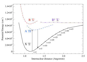
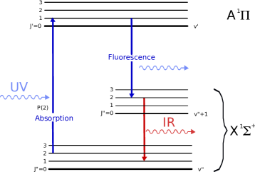
Figure 1: CO energy potential curves on the left and a schematic of the UV fluorescence mechanism on the right. We are concerned with transitions between the ground electronic state $X^{1}\Sigma^{+}$ and the electronic excited state $A^{1}\Pi$. The arrows show a possible UV-fluorescence pumping from a ground electronic level ($X^{1}\Sigma^{+}$) at $v^{\prime\prime}=1$ to a level in the electronic state $A^{1}\Pi$, followed by a de-excitation to the level $v^{\prime\prime}=2$ in the ground electronic state. The value for the curves are taken from Cooper & Kirby (1987).

Table 1: Höln-London factors taken from Morton & Noreau (1994).

	$P$	$Q$	$R$
	$J^{\prime}=J^{\prime\prime}-1$	$J^{\prime}=J^{\prime\prime}$	$J^{\prime}=J^{\prime\prime}+1$
${}^{1}\Sigma$-${}^{1}\Sigma$	$J^{\prime\prime}$	…	$J^{\prime\prime}+1$
	$J^{\prime}+1$	…	$J^{\prime}$
${}^{1}\Pi$-${}^{1}\Sigma$	$J^{\prime\prime}-1$	$2J^{\prime\prime}+1$	$J^{\prime\prime}+2$
	$J^{\prime}$	$2J^{\prime}+1$	$J^{\prime}+1$

2.2 Collisional data

Although CO is one of the most studied interstellar molecules with a large amount of experimental and theoretical collision rates available, the lack of completeness of any individual study obliged us to use scaling laws to fill the gaps. Since protoplanetary discs show a large range of physical and chemical properties, we need to consider collisions of CO with H, He, H₂, and electrons. In the rest of the section, we will first review existing theoretical and experimental collision rates before discussing the strengths and limitations of scaling laws.

2.2.1 CO-H collision rates

The $v$=1$\rightarrow$0 CO-H de-excitation rate coefficients were first measured by Millikan & White (1963) in shock-tube experiments. Subsequent works include the shock-tube experiments by von Rosenberg et al. (1971), Glass & Kironde (1982), and more recently Kozlov et al. (2000) (between 2000 and 3000 K). Shock-tube experimental measurements are de-excitation timescales,which can be fitted in terms of the Landau-Teller rate coefficients in cm³ s^-1 (Ayres & Wiedemann 1989):

$$k_{v^{\prime}\rightarrow v^{\prime\prime}}=4.2\times 10^{-19}\frac{\exp{[B-0.0069A\beta^{1/3}]}}{\beta(1-e^{-\beta})}$$ (1)

with $\beta=E_{\rm v=1}/T$ and the values for $A$ and $B$ given in Table 2. Neufeld & Hollenbach (1994) gave a simple formula that fits the shock-tube data for $T>$ 300 K:

$$k_{v}(1\rightarrow 0)=7.9\times 10^{-13}T\exp{(-1208T)}.$$ (2)

This formula supersedes an older one given by Hollenbach & McKee (1979):

$$k_{v}(1\rightarrow 0)=3\times 10^{-12}\sqrt{T}e^{-(2\times 10^{3}/T)^{3.43}}e^{-3080/T}.$$ (3)

Experimental values for transitions other than the $v$=1$\rightarrow$0 are not available.

Table 2: Landau-Teller coefficients for CO-partner collisions derived from shock-tube experiments.

Partner	$A$	$B$	Ref.
H	3	18	1
H	53	19	2
H	188.9	36	3, 4
H2	64	19.1	1
He	87	19.1	4

Balakrishnan et al. (2002) performed quantal scattering computations for rotational and band-averaged vibrational collision rates between CO and hydrogen atoms. They used the close-coupling method for the rotational transitions and the infinite order sudden approximation (IOS, Flower 2007) for the vibrational transitions for a large range of gas temperatures (5 $<$ $T$ $<$ 3000 K). The IOS approximation reduces the computational effort but is strictly valid only for energetic collisions, i.e. $\Delta E\ll kT$, where $\Delta E$ is the energy difference between two levels. The close-coupling computations were done for rotational levels up to $J$=7. The vibrational transition rates were computed up to $v=$ 4.

Figure 2 shows the different rate coefficients. The most striking feature is the large dispersion (a few orders of magnitude) between the sources. Ayres & Wiedemann (1989) chose the values of Glass & Kironde (1982), which are much larger than the older values of von Rosenberg et al. (1971). However, recent measurements by Kozlov et al. (2000) reproduced the values of von Rosenberg et al. (1971). Interestingly, the theoretical values calculated by Balakrishnan et al. (2002) are much closer to the values of Glass & Kironde (1982) and are best approximated by the formula of Neufeld & Hollenbach (1994). One possible reason for the large discrepancies is the reactivity of CO with atomic hydrogen (an open shell species), which can falsify the measurements. We chose to use the theoretical rates by Balakrishnan et al. (2002).

Figure 2: Vibrational de-excitation ($v$=1$\rightarrow$0) rate coefficients of CO by collisions with H (in cm³ s^-1). The large discrepancies between the experimental values may stem from the reactivity of H-atoms with CO. We adopted the theoretical rates from Balakrishnan et al. (2002), which match the experimental values of Glass & Kironde (1982) (plus signs).

2.2.2 CO-He collision rates

Cecchi-Pestellini et al. (2002) computed rotational and vibrational rate de-excitation coefficients of CO in collision with He. The rotation rate coefficients in the ground vibrational level are computed by the quantal close-coupling method. The vibrational rates are computed for 500$\leq$ $T$ $\leq$ 1300 K using the IOS approximation. Krems (2002) calculated quantum-mechanically ro-vibrational rate coefficients for 35 $\leq$ $T$ $\leq$ 1500 K. Rates were computed by Flower (2012) and Reid et al. (1995). The experimental fit coefficients of Millikan (1964) are given in Table 2. Wickham-Jones et al. (1987) reported experimental data from the PhD thesis of Chenery (1984), who measured rates down to 35 K. The experimental rate coefficients are compared to the theoretical values in Fig. 3. The theoretical values of Cecchi-Pestellini et al. (2002) are a factor $\sim$ 2 smaller than the experimental values, whereas the values computed by Krems (2002) match the shock-tube data down to $T$= 300 K. The formula 1 that fits the experimental shock-tube data under-predicts the values for $T\leq$ 300 K. We adopted the values of Krems (2002) up to $T$= 1500 K and those of Cecchi-Pestellini et al. (2002) above $T$= 1500 K. The rate coefficients for CO in collisions with He are around three orders of magnitude smaller than the collision rates with H. This behaviour can be explained by the fact that He is a close-shell species.

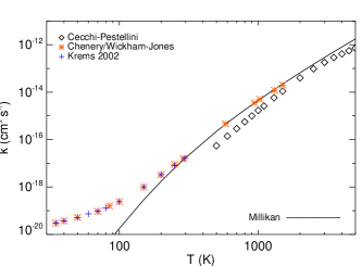
Figure 3: Vibrational de-excitation ($v$=1$\rightarrow$0) rate coefficients of CO by collisions with He (in cm³ s^-1). We adopted in this study the rates of Krems (2002) at temperatures $<$ 1500 K (plus signs) and those of Cecchi-Pestellini et al. (2002) at very high temperatures ($>$ 1500 K, diamonds).

2.2.3 CO-H₂ collision rates

In the case of collisional excitation of CO by H₂, we need to consider the collisions with ortho-H₂ and para-H₂ separately. Yang et al. (2010) computed with the close-coupling method rates for temperatures between 1 and 3000 K involving ground vibrational CO transitions and with rotational levels up to $J$=40.
Rates for vibrational transitions are scarcer and are given averaged over the rotational levels. Between 30 and 70 K, Reid et al. (1997) showed experimental and theoretical rates for the CO v=1$\rightarrow$0 transition. Between 70 and 290 K, rates derived from shock-tube experiments are available (Hooker & Millikan 1963; Andrews & Simpson 1975, 1976; Glass & Kironde 1982). At temperatures higher than 300 K, we can assume that the Landau-Teller law is valid and expand the shock-tube rates to a few thousand K (Ayres & Wiedemann 1989). Neufeld & Hollenbach (1994) provided a convenient analytical expression of the shock-tube data ($T>$290 K):

$$k_{v}(1\rightarrow 0)=4.3\times 10^{-14}T\exp{(-68T^{1/3})}.$$ (4)

Alternatively, one can use the Landau-Teller formula with the values in Table 2.

In Fig. 4, we compare the two shock-tube experimental rate coefficients, the experimental and theoretical values of Reid et al. (1997), and our adopted fit

$$k_{v}(1\rightarrow 0)=5\times 10^{-19}T\exp{(2\times 10^{-3}T)},$$ (5)

for $T\leq$ 300 K and the fit to the Hooker & Millikan (1963) data by Neufeld & Hollenbach (1994) above 300 K. We notice a large discrepancy between the experimental and theoretical rates at low temperatures. The shock-tube data are consistent with each other. It is known that the rate extrapolations to lower temperatures with the Landau-Teller law may not be correct. Collisions with H are around two orders of magnitude more effective than collisions with H₂ at all temperatures.

Figure 4: Vibrational de-excitation ($v$=1$\rightarrow$0) rate coefficients of CO by collisions with H₂ (in cm³ s^-1). Normal H₂ is a mix of o-H₂ and p-H₂ with an ortho-to-para ratio at LTE.

2.2.4 CO-electron collision rates

The collision excitation and de-excitation rates of CO by electrons for rotational transitions are computed using the theory of Dickinson et al. (1977) based on the Born approximation for $\Delta J=\pm$ 1 (see also Randell et al. 1996). We adopted a rotational constant $B_{{\rm CO}}=$ 1.922529 cm^-1, a centrifugal distortion $D_{{\rm CO}}=$ 6.1210779 $\times$ 10^-6 cm^-1, and a dipole moment of 0.112 Debye. Ristić et al. (2007) measured the vibrational rates of CO by collisions with electrons for vibrational levels up to ten. Morgan & Tennyson (1993) also computed cross sections for vibrational transitions. Thompson (1973) gave a simple formula for the v=1$\rightarrow$0 rate

$$k_{v}(1\rightarrow 0)=1.4\times 10^{-9}{\beta}^{-1/2}\left(1+\beta+19e^{-3.22\beta}(1+4.22\beta)\right),$$ (6)

where again $\beta=E_{\rm v=1}/T$. An alternative formula is given by Draine & Roberge (1984)

$$k_{v}({\rm v}=1\rightarrow 0)=1.9\times 10^{-11}\sqrt{T}\\ \left(\sqrt{\frac{2420}{T}}+10\sqrt{1+\frac{10500}{T}}\exp{\left(-\frac{10210}{T}\right)}\right).$$ (7)

Finally, we propose our own analytical formula, which fits the values of Ristić et al. (2007)

$$k_{v}({\rm v}=1\rightarrow 0)=1.9\times 10^{-11}T^{1/3}\\ \left(\left(\frac{2000}{T}\right)^{1/3}+50\sqrt{1+\frac{70000}{T}}\exp{\left(-\frac{10210}{T}\right)}\right)\\ \exp{(-4.5\times 10^{-5}T)}.$$ (8)

The measurements for the $v$=1$\rightarrow$0 transition are shown in Fig. 5 and compared to the three analytical fitting formulae. The Thompson (1973) formula deviates significantly from the experimental data. We used a combination of formula (8), which fits the experimental data relatively well down to 400 K.Below 400 K, we adopted a flat rate coefficient.

Figure 5: Vibrational de-excitation ($v$=1$\rightarrow$0) rate coefficients of CO by collisions with electrons (in cm³ s^-1).

2.3 Rate coefficient scaling laws

The current experimental and theoretical works do not provide all the rate coefficients needed to model the CO statistical ro-vibrational population of the ground $X^{1}\Sigma^{+}$ and excited $A^{1}\Pi$ electronic levels. Therefore, we have to resort to extrapolation and scaling laws to fill the gaps.

2.3.1 Extrapolating rotational transition rates

A few extrapolating laws attempt to estimate rates from existing ones. We used the energy-corrected sudden (ECS) scaling law with a hybrid exponential power-law for the base ($k_{{\rm J^{\prime\prime}}\rightarrow 0}$) rates (Depristo et al. 1979; Depristo 1979; Green 1993). Goldflam et al. (1977) showed that rates between any levels can be derived knowing the rates to the ground level within the IOS approximation. To overcome the limitation of collision energies greater than the level energy differences, Depristo et al. (1979) proposed a correction for the inelasticity and finite collision duration effects using second-order perturbation theory for low-collision energies (i.e. for collisions at low temperatures). A de-excitation ($J^{\prime}>J^{\prime\prime}$) rate is given by the ESC-EP (energy-corrected sudden scaling law with a hybrid exponential power-law for the base rates) formula:

$$k_{0,J^{\prime}\rightarrow 0,J^{\prime\prime}}=(2J^{\prime\prime}+1)\exp{\left[\frac{(E_{J^{\prime}}-E_{J^{\prime\prime}})}{kT}\right]}\Omega^{2}_{J^{\prime}}\\ \times\sum_{L}(2{L}+1)\Omega^{-2}_{L}\left(\begin{array}[]{ccc}{J^{\prime}}&{L}&{J^{\prime\prime}}\\ 0&0&0\end{array}\right)^{2}k_{{0,J^{\prime}}\rightarrow{0,0}},$$ (9)

where

$$\left(\begin{array}[]{ccc}{J^{\prime}}&{L}&{J^{\prime\prime}}\\ 0&0&0\end{array}\right)$$ (10)

is the Wigner 3-$j$ symbol and $E_{J^{\prime}}$ and $E_{J^{\prime\prime}=J^{\prime}-1}$ are the upper and lower level energy, respectively. The correction factor introduced by Depristo et al. (1979) is defined by

$$\Omega_{J^{\prime}}=\frac{1}{1+\tau_{J^{\prime}}/6},$$ (11)

with

$$\tau_{J^{\prime}}=0.065\omega_{J^{\prime}}l_{c}(\mu/T)^{1/2},$$ (12)

where $\mu$ is the reduced mass in atomic mass units, $\omega_{J^{\prime}}$ is the inelasticity to the next lowest level ($E_{J^{\prime}}-E_{J^{\prime\prime}=J^{\prime}-1}$) in cm^-1, and $l_{c}$ is an adjustable scaling length in Å. We adopted $l_{c}$=3 Å (Schöier et al. 2005). The ESC formula is recovered for $l_{c}$=0 Å.

The scaling law requires the knowledge of the base rates ($J\rightarrow 0$). Collision rates with hydrogen atoms to the ground level are known for $J$ up to 7, with H₂ up to 40, and only for $J$=1$\rightarrow$0 for electrons. Further estimates of the rates to the ground level are needed. The ESC-EP model provides an approximation for rates to the ground level (Green 1993; Millot 1990):

$$k_{{0,J^{\prime}}\rightarrow{0,0}}=A(T)\left[J^{\prime}(J^{\prime}+1)\right]^{-\gamma}\exp{(-\beta E_{J^{\prime}}/kT)},$$ (13)

where $A(T)$, $\gamma$, and $\beta$ are free parameters, which are estimated by fitting equation 13 to the existing data using a least-square solver for over-constrained systems. We performed the extrapolation for collisions with o-H₂, p-H₂, He, and H but not with electrons. An example of extrapolated rate coefficients is shown in Fig. 6.

Figure 6: Extrapolated CO – o-H₂ pure rotational rate coefficients. The x-axis corresponds to the upper level energy in Kelvin.The diamonds are rates from Yang et al. (2010).

2.3.2 Extrapolating vibrational transition rates

The extrapolation of an existing rate to low temperature was performed by fitting the available rates to the formula

$$k_{v}=a\times\exp{(T+b)},$$ (14)

where $a$ and $b$ are the two fitting parameters.

The extrapolation of rates between two vibrational levels without any known rate follows physically motivated scaling laws. Based on the initial work of Procaccia & Levine (1975), Chandra & Sharma (2001) proposed using the Landau-Teller relationship for transitions between adjacent states ($\Delta{\rm v}=1$)

$$k_{v}(v^{\prime}\rightarrow v^{\prime}-1)=v^{\prime}k_{v}(1\rightarrow 0),$$ (15)

and for $\Delta{\rm v}>1$:

$$k_{v}(v^{\prime}\rightarrow v^{\prime\prime})=\frac{2(v^{\prime\prime}-1)+1}{2(v^{\prime}-2)+1}v^{\prime}k_{v}(1\rightarrow 0)$$ (16)

Elitzur (1983) argued for a different formulation

$$k_{v}(v^{\prime}\rightarrow v^{\prime\prime})=(v^{\prime}-v^{\prime\prime})k_{v}(1\rightarrow 0)\\ \exp{\left(-(v^{\prime}-v^{\prime\prime}-1)\frac{1.5E_{v}/kT}{1+1.5E_{v}/kT}\right)}.$$ (17)

For $\Delta v=1$ ($v^{\prime\prime}=v^{\prime}-1$), this last formula reduces to

$$k_{v}(v^{\prime}\rightarrow v^{\prime}-1)=k_{v}(1\rightarrow 0).$$ (18)

Scoville et al. (1980) argued that the probabilities of collision-induced vibrational transitions are proportional to the corresponding radiative transition matrix elements (Born-Coulomb long range interaction). Therefore, the vibrational de-excitation rate coefficients from $v^{\prime}$ to $v^{\prime\prime}$ can be derived from the $v=1\rightarrow 0$ rate coefficients:

$$k_{v}(v^{\prime}\rightarrow v^{\prime\prime})=\frac{A_{v^{\prime}v^{\prime\prime}}}{A_{10}}k_{v}(1\rightarrow 0),\\$$ (19)

where $A_{v^{\prime}v^{\prime\prime}}$ is the vibrational band transition probabilities. The three formulations give quite different rate estimates. In order to choose which one is the most appropriate, we compared the predictions with detailed calculations and/or experimental values.

Figure 7 shows the rate coefficient ratios for transitions between adjacent levels in collisions with atomic hydrogen using the detailed calculation of Balakrishnan et al. (2002). The ratios are grouped around one with a small spread. The rate coefficient ratios suggest that the expansion rules proposed by Elitzur (1983) are more appropriate to expand the detailed rate coefficients.

The rate coefficient ratios for CO-He collisions vary dramatically with temperature (Fig. 8). For temperatures below 1000 K, the ratios are close to $2\times v^{\prime}$, a value that corresponds neither to the Chandra & Sharma (2001) prescription ($=v^{\prime}$) nor to that championed by Elitzur (1983) (=1). We chose to use the Chandra & Sharma (2001) for $\Delta v>$1 and the factor $2\times v^{\prime}$ for $\Delta v=$1.

The choice is open concerning the rules to apply to estimate the rate coefficients between CO and H₂ and between CO and electrons other than $v^{\prime\prime}$=1$\rightarrow$0. We chose to use the same combination of scaling rules as for CO-He collisions. We estimate the scaling rules to provide rates correct within an order of magnitude.

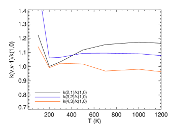
Figure 7: Vibrational de-excitation rate coefficient ratios $k$(v’$\rightarrow$v’-1)/$k$(1$\rightarrow$0) of CO by H. Rate coefficients are taken from Balakrishnan et al. (2002).

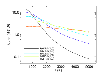
Figure 8: Vibrational de-excitation rate coefficient ratios $k$(v’$\rightarrow$v’-1)/$k$(1$\rightarrow$0) of CO by He. Rate coefficients are taken from Krems (2002).

2.3.3 Estimating ro-vibrational transition rates

The vibrational rates are averaged over all ro-vibrational transitions. To obtain individual rates between ro-vibrational states, we apply the method described in Faure & Josselin (2008). This method assumes a complete decoupling of rotational and vibrational levels. The state-to-state ro-vibrational rates are related to the corresponding rates for the pure rotational transitions in the ground vibrational state:

$$k_{v^{\prime},J^{\prime}\rightarrow v^{\prime\prime},J^{\prime\prime}}=P_{v^{\prime}v^{\prime\prime}}k_{0,J^{\prime}\rightarrow 0,J^{\prime\prime}}.$$ (20)

The factor $P_{{\rm v^{\prime}v^{\prime\prime}}}$ is defined as

$$P_{v^{\prime}v^{\prime\prime}}(T)=\frac{k_{v^{\prime}\rightarrow v^{\prime\prime}}\sum_{J^{\prime}}g_{J^{\prime}}\exp{(-E_{v^{\prime},J^{\prime}}/kT)}}{\sum_{J^{\prime}}\left(g_{J^{\prime}}\exp{(-E_{v^{\prime},J^{\prime}}/kT)}\sum_{J^{\prime\prime}}k_{0,J^{\prime}\rightarrow 0,J^{\prime\prime}}\right)}.$$ (21)

This formula ensures detailed balance.

2.3.4 Approximating electronic transition collision rates

In the absence of collision rates connecting the ground $X^{1}\Sigma^{+}$ to the $A^{1}\Pi$ electronic levels, we adopted the rough values for CO-electron collision rates provided by the $\bar{g}$ approximation. The $\bar{g}$ (van Regemorter 1962) approximation relies on the Born-dipole (also called Born-Coulomb) long-range interaction approximation and relates the collision strength to the transition probability and wavelength for allowed transitions (Itikawa 2007). The Born-dipole approximation is valid for species with a permanent dipole, which is the case for CO ($\mu$=0.122 Debye). The collision rate for allowed transitions is given by

$$k_{ul}=\frac{8.6291\times 10^{-6}}{g_{u}\sqrt{T}}\Gamma$$ (22)

For neutrals, the g-bar value can be approximated by

$$\bar{g}\simeq(kT/h\nu)$$ (23)

The collision strength $\Gamma$ is related to g-bar by

$$\Gamma=2.388\times 10^{-6}\lambda_{\mu\rm m}^{3}g_{u}A_{ul}\bar{g}$$ (24)

The approximation provides rate coefficients correct within an order of magnitude.

2.3.5 Combining theoretical, experimental, and estimated rates

The resulting CO rate matrix after combining all existing and estimated rates is complete in the sense that all ro-vibrational levels in the ground electronic state connected by a radiative transition are also connected by collisions. Therefore all levels in the ground electronic levels can be populated in LTE at very high densities and temperatures. We have neglected the radiative and collisional transitions between levels in excited electronic states since radiative transitions to the ground electronic state are very fast. The ”completeness” is required to ensure that we don’t artificially create sub-thermally populated levels. The methodology described above was implemented in the radiative photochemical code ProDiMo. The main collisional partner in ro-vibrational transitions is the atomic hydrogen by a few orders of magnitude.

3 CO fundamental and hot-band emission from Herbig Ae discs

3.1 The ProDiMo code

A detailed description of the code can be found in (Woitke et al. 2009). Subsequent additions to the code are documented in Kamp et al. (2010), Thi et al. (2011), and Woitke et al. (2011). Although not used in this study X-ray heating and X-ray chemistry are included in ProDiMo (Aresu et al. 2011). We deal in this paper with the excitation mechanisms of the CO ro-vibrational levels and do not attempt to fit actual observations.

3.2 Disc model description

We chose to model two representative discs, which can be found around Herbig Ae stars. Our generic star has an effective temperature of 8600 K, a mass of 2.2 M_⊙, and luminosity of 32 L_⊙. We have no intention to fit a particular object in this study. The input stellar spectrum is taken from the PHOENIX database of stellar spectra (Brott & Hauschildt 2005). The disc model parameters are summarized in Table 3. The disc geometry is described by a single zone power-law surface-density profile with index $\epsilon$, an inner radius $R_{\mathrm{in}}$, an outer radius $R_{\mathrm{out}}$, a disc gas mass $M_{\mathrm{disc}}$, and a standard gas-to-dust mass ratio $\Delta$ of 100 for all the discs. The inner radius was set to two values to model the presence of an inner disc hole and its effects on the CO ro-vibrational emissions.

Table 3: Disc and CO parameters. The parameters are defined in Woitke et al. (2009)

stellar mass	$M_{*}$	2.2 M⊙
stellar luminosity	$L_{*}$	32 L⊙
effective temperature	$T_{\mathrm{eff}}$	8600 K
distance	$d$	140 pc
disc inclination	$i$	0 ° (face-on)
total disc mass	$M_{\mathrm{disc}}$	10-2, 10-4 M⊙
disc inner radius	$R_{\mathrm{in}}$	1, 20 AU
disc outer radius	$R_{\mathrm{out}}$	300 AU
vert. column density index	$\epsilon$	1
inner rim soft edge		on
gas to dust mass ratio	$\delta$	100
dust grain material mass density	$\rho_{\mathrm{dust}}$	3.5 g cm-3
minimum dust particle size	$a_{\mathrm{min}}$	0.05 $\mu$m
maximum dust particle size	$a_{\mathrm{max}}$	1000 $\mu$m
composition		ISM silicate
dust size distribution power-law	$p$	3.5
H2 cosmic ray ionization rate	$\zeta_{\mathrm{CR}}$	1.7 $\times$ 10 -17 s-1
ISM UV field w.r.t. Draine field	$\chi$	1.0
abundance of PAHs relative to ISM	$f_{\rm PAH}$	0.1
$\alpha$ viscosity parameter	$\alpha$	0.0
turbulence width	$\delta v$	0.15 km s-1
reference scale height	$H_{0}$	15 AU
reference radius	$R_{0}$	100 AU
flaring index	$p$	1.2
CO $X^{1}\Sigma^{+}$	rot. levels	50
CO $A^{1}\Pi$	rot. levels	50
CO $X^{1}\Sigma^{+}$	vib. levels	up to 9
CO $A^{1}\Pi$	vib. levels	up to 9

The dust grains are defined in both discs by their composition (astronomical silicates, Laor & Draine 1993) and their size distribution (a power-law ranging from $a_{\mathrm{min}}$ to $a_{\mathrm{max}}$). We did not iterate on the vertical hydrostatic profile but used instead a power-law $H=H_{0}(R/R_{0})^{-p}$ to model the gas scale-height $H$. We chose to model two flaring discs (flaring index $p$=1.2) because observations suggest that the CO levels populated by UV-fluorescence pumping seem to occur in flaring discs.

The two discs differ from each other only in the total (gas+dust) disc mass $M_{\mathrm{disc}}$. The first disc has a mass consistent with the typical solar nebula mass of 0.01 M_⊙, while the second disc is more akin to an object in transition from a primordial gas-rich disc to a secondary debris disc with a total mass of 10^-4 M_⊙. The choice of the two masses is motivated by the possibility to assess the effects of infrared and UV fluorescence on the CO population in discs with vastly different density structures. The discs are assumed passively heated only (i.e. without viscous heating: $\alpha=$ 0), and we do not consider X-ray heating because the X-ray luminosity is generally low compared to the UV luminosity in Herbig Ae stars. X-ray heating and chemistry can play an important role in discs around T Tauri stars (Aresu et al. 2011, 2012; Meijerink et al. 2012).

The main source of heating for the gas is the stellar UV via photoelectric effects on polycyclic aromatic hydrocarbons (PAHs) assumed here to be circumcoronenes (C₅₄H₁₈). The abundance of PAHs is assumed at 10% of the standard interstellar abundance ($f_{\mathrm{PAH}}=0.1$).

The gas and dust were assumed well-mixed with no dust settling. A detailed discussion on the heating and cooling in HerbigAe discs can be found in Kamp et al. (2010).

The continuum radiative transfer and dust thermal balance are calculated in two dimensions using the long-characteristic method (Woitke et al. 2009; Thi et al. 2011). The radiative transfer numerical implementation was benchmarked against other radiative transfer codes (Pinte et al. 2009). The gas temperatures were computed by balancing the heating and cooling (mostly radiative) processes. The CO self-shielding against photodissociation uses factors interpolated from values in look-up tables (Visser et al. 2009).

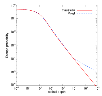
Figure 9: Escape probability for a semi-infinite slab. We adopted $a=10^{-3}$ for illustration.

Table 4: CO LTE rotational temperature and vibrational temperature for the UV/no-UV models derived from analyzing the CO fundamental emission rotational diagrams. max($T_{\mathrm{dust}}$) is the maximum dust temperature attained in the disc. n.a. means not available.

Model	$M_{\mathrm{disc}}$	$R_{\mathrm{in}}$	$A^{1}\Pi$	$X^{1}\Sigma^{+}$	UV	$T_{\mathrm{rot}}^{\mathrm{LTE}}$	$T_{\mathrm{vib}}$	max($T_{\mathrm{dust}}$)
			number of	number of	pumping?	$v=1\rightarrow 0$	v=0,…,5
	(M⊙)	(AU)	vib. levels	vib. levels		(K)	(K)	(K)
1a	10-2	1	9	9	yes	777	1413	857
1b	10-2	1	0	9	no	777	941-1413	857
1c	10-2	1	0	5	no	n.a.	1413	857
1d	10-2	1	0	2	no	n.a.	n.a.	857
1e	10-2	1	0	1	no	n.a.	n.a.	857
2a	10-2	20	9	9	yes	655	2025	184
2b	10-2	20	0	9	no	655	576	184
3a	10-4	1	9	9	yes	907	1740	815
3b	10-4	1	0	9	no	907	858-1192	815
3c	10-4	1	0	5	no	n.a.	858	815
3d	10-4	1	0	2	no	n.a.	n.a.	815
3e	10-4	1	0	1	no	n.a.	n.a.	815
4a	10-4	20	9	9	yes	658	3177	172
4b	10-4	20	0	9	no	658	560	172
5a	10-3	1	9	9	yes	750	1438	838
5b	10-3	1	0	9	no	750	1096	838
6a	10-3	5	9	9	yes	772	1731	352
6b	10-3	5	0	9	no	772	1000	352
7a	2.5 $\times$ 10-3	5	9	9	yes	734	1628	357
7b	2.5 $\times$ 10-3	5	0	9	no	734	915	357
8a	5 $\times$ 10-3	5	9	9	yes	726	1575	360
8b	5 $\times$ 10-3	5	0	9	no	726	872	360

CO ro-vibrational transitions have moderate Einstein probabilities ($A$=1-10 s^-1) so that the line transfer occurs in the Doppler core of the line profile. On the other hand, UV-fluorescence pumping occurs via electronic transitions ($A^{1}\Pi$–$X^{1}\Sigma^{+}$) with high Einstein probabilities ($A$=10⁴-10⁷ s^-1) and thus with large natural line width. The line core becomes quickly optically thick (line self-shielding) with the UV line transfer happening in the Lorentzian wings of the line. Therefore the use of the Voigt profile in the line transfer is warranted.

The CO levels are computed using a 1+1D escape probability method for Voigt line profiles. We adapted the analytical formulation of Apruzese (1985) to match the formulation in Woitke et al. (2009) at low optical depths and small intrinsic line widths. At high optical depth, the escape probability $\beta$ varies as $\tau^{-1/2}$ (Voigt profile) instead of $\tau^{-1}$ (Gaussian profile):

$$\beta=\left\{\begin{array}[]{ll}0.5(1+1.5\tau)^{-1}&\mathrm{if\ }\tau\leq 1\\ 0.25\tau^{-1.15}&\mathrm{if\ }1<\tau<\tau_{c}\\ 0.25\tau^{-0.5}\tau_{c}^{-0.65}&\mathrm{if\ }\tau>\tau_{c},\\ \end{array}\right.$$ (25)

where $a$ is defined as $\Gamma/(4\pi\Delta\nu_{D})$ and $\tau_{c}$ is the critical optical depth and is defined as $0.83/(a(1+\sqrt{a}))$. The sum of the natural and collisional width is $\Gamma$ while the effective Doppler width is $\Delta\nu_{D}$ (Rybicki & Lightman 1986). The escape probability function for a Voigt line profile is illustrated in Fig. 9 for the case $a=10^{-3}$. In addition to the UV line shielding, dust grains contribute strongly to the UV flux attenuation. The main limitation in using the escape probability technique is that it does not take overlapping line effects into account.

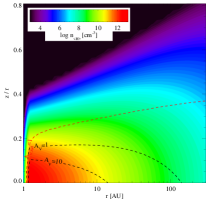
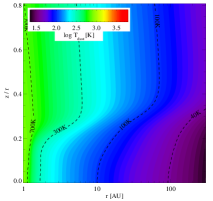
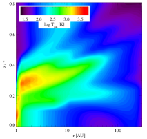
Figure 10: Density, $T_{\mathrm{dust}}$, and $T_{\mathrm{gas}}$ structures for model 1a. The contours in black dashed lines in the density panel show the location of $A_{\mathrm{V}}$=1 and 10 from $z=\infty$. The red dashed lines mark the location of the radial $A_{\mathrm{V}}$=1 calculated from $R_{\mathrm{in}}$. In the middle panel various dust temperature contours are shown in black dashed lines. In our models, $T_{\mathrm{dust}}$ and $T_{\mathrm{gas}}$ are not equal.

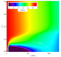
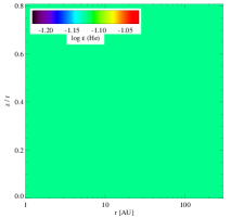
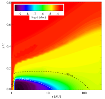
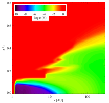
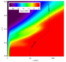
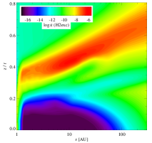
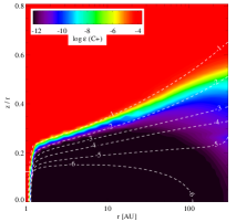
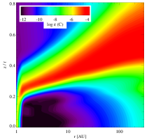
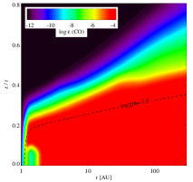
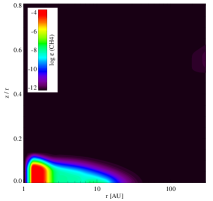
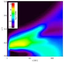
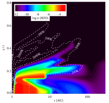
Figure 11: Model 1a $\chi$ structures and abundances relative to H-nuclei for atomic He, electron, H, H₂, H₂exc ($v>$0), C⁺, C, CO, CH₄, OH, and H₂O. The contour plots in the ionized carbon abundance plot show $\log(\chi/n$), where $\chi$ is the enhancement with respect to the interstellar UV and $n$ the total number of H-nuclei. In a few panels, dust temperature ($T_{\mathrm{d}}$), gas temperature (water abundance panel), or extinction $A_{\mathrm{V}}$ contours are overplotted by dashed lines.

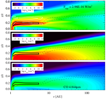
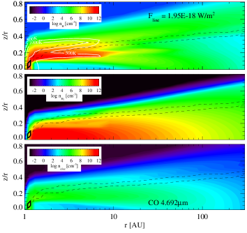
Figure 12: Location of the CO $v=1-0$ $J=19-18$ $P$(19) at 4.844 $\mu$m and CO $v=4-3$ $J=20-19$ $P$(20) at 4.692 $\mu$m line emissions for the $M_{\mathrm{disc}}$=10^-2 M_⊙, $R_{\mathrm{in}}$=1 AU disc models with (left panels, model 1a) and without (right panels, model 1b) UV-pumping. The solid black contours in the CO density panels encompass the regions that emit 49% of the fluxes. The black dashed-line contours contain 70% of the fluxes in the vertical direction. The white contours are at gas temperatures of 500 and 1000K. Each panel is divided into three sub-panels. The upper sub-panels show in color scale the atomic hydrogen density structure, the middle-panels show the molecular hydrogen density structure, and the lower-panels show the electron density structure.

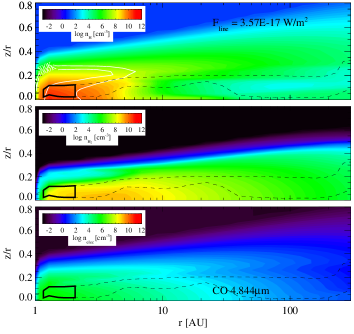
Figure 13: Similar to Fig. 12 but for the $M_{\mathrm{disc}}$=10^-4 M_⊙, $R_{\mathrm{in}}$=1 AU disc models (3a and 3b).

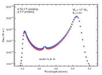
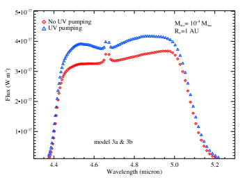
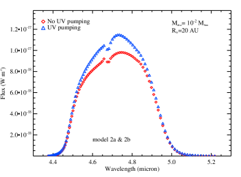
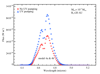
Figure 14: CO $v=1-0$ continuum-subtracted line fluxes. The blue triangles show the fluxes for models with UV-pumping, whereas the red diamonds show the fluxes for models without UV-pumping.

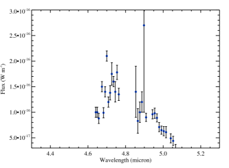
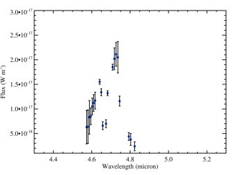
Figure 15: CO SLED from AB~Aur (left panel) and HD~141569A discs (with the fluxes scaled to a distance of 140 pc, right panel). Both observations are taken from Brittain et al. (2003).

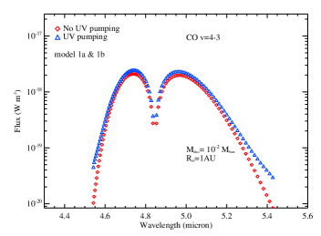
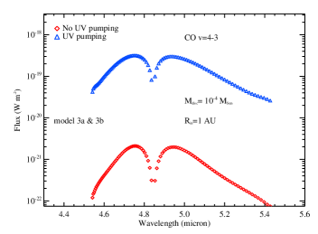
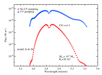
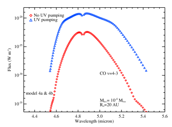
Figure 16: CO $v=4-3$ continuum-subtracted line fluxes. The blue triangles show the fluxes for models with UV-pumping whereas the red diamonds show the fluxes for models without UV-pumping.

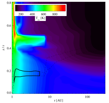
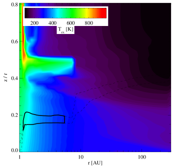
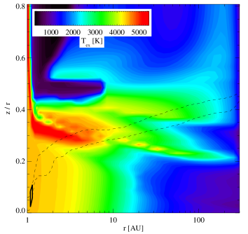
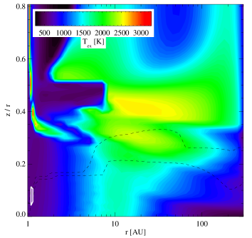
Figure 17: . Excitation temperatures $T_{\mathrm{ex}}$ between the upper and lower level of the CO $v=1-0$ $P$(19) transition at 4.844 $\mu$m $v=1,J=19$ (upper two panels) and that of the CO $v=4-3$ $P$(20) transition at 4.692 $\mu$m $v=4,J=20$ (lower two panels) transitions for the $M_{\mathrm{disc}}$=10^-2 M_⊙, $R_{\mathrm{in}}$=1 AU disc models with (left panels, model 1a) and without (right panels, model 1b) UV-pumping. The solid contours (in white or black) in the CO density panels encompass the regions that emit 49% of the fluxes. The black dashed-line contours contain 70% of the fluxes in the vertical direction. The white contours are at gas temperatures of 500 and 1000K.

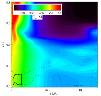
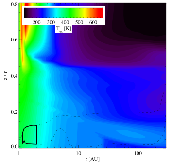
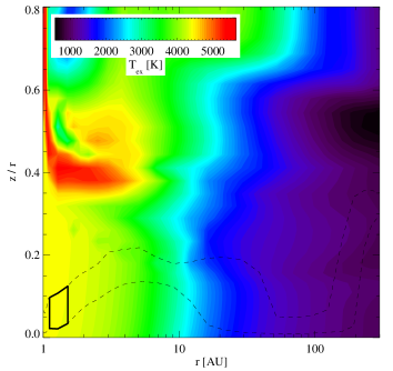
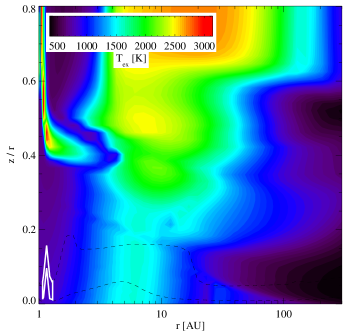
Figure 18: . Similar to Fig. 17 but for the $M_{\mathrm{disc}}$=10^-4 M_⊙, $R_{\mathrm{in}}$=1 AU disc models (3a and 3b).

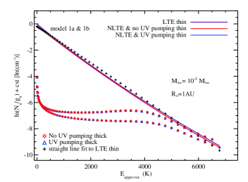
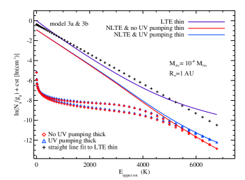
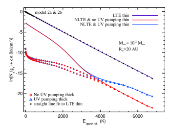
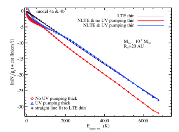
Figure 19: Disc model CO $v=1$ population diagrams: LTE and NLTE with and without UV pumping in the optically thin case (solid lines) and optically thick case (symbols). All the data have been normalized to the $J$=0 population in LTE. The blue diamonds correspond to the column densities after line transfer in models with UV pumping whereas the red triangles correspond to column densities in line-transfer model results without UV pumping. The LTE populations are fitted by straight lines (black plus signs). The separations between $P-$ and $R-$ branches are clearly seen in the NLTE optically thick cases.

Excited vibrational levels can also be populated by the absorption of an IR photon emitted by the star and the dust grains, a phenomenon called IR pumping. We also checked the effect of IR pumping on the vibrational ground rotational population by modelling two discs with $R_{\mathrm{in}}$=1 AU, one with $M_{\mathrm{disc}}$=10^-2 M_⊙ (models 1c, 1d, and 1e) and with $M_{\mathrm{disc}}$=10^-4 M_⊙ (models 3c, 3d, and 3e). For each disc model, we computed the rotational level population by taking into account: (1) ro-vibrational levels up to $v$=5 (models 1c and 3c), (2) ro-vibrational levels with $v$=0 and $v$=1 (models 1d and 3d), and (3) the rotational levels in the ground vibrational only (models 1e and 3e).

In total, we ran four series of models with and without the electronic levels and with different numbers of vibrational levels to assess the importance of UV fluorescence and IR pumping (see Table 4). Complete spectra from four to five microns are generated for discs seen face-on (zero inclination).

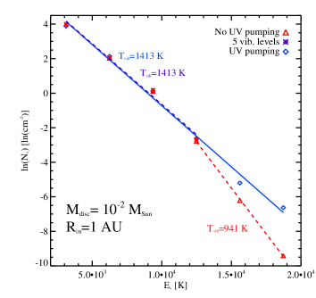
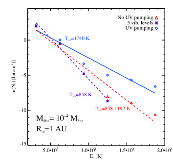
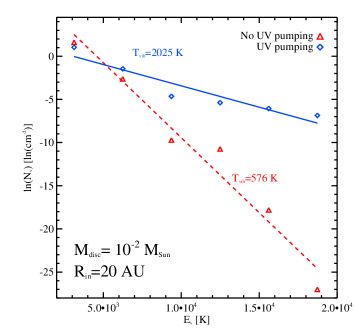
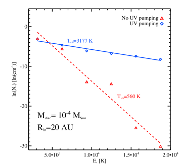
Figure 20: CO vibrational diagram with and without UV pumping for the four models. We used the $v$=1–6 population after line radiative transfer. The blue diamonds correspond to models with UV pumping whereas the red triangles correspond to models without UV pumping. The purple stars are models without UV pumping and 5 vibrational levels. Straight lines have been fitted to each dataset. The derived vibrational temperatures are indicated in each panel. The blue lines are for models with UV-pumping whereas the red dashed-lines are for models without UV-pumping. In the upper left panel, massive disc including UV-pumping show the same vibrational temperature ($T_{\mathrm{vib}}$=1413 K) with either 5 or 9 electronic ground-state vibrational levels included in the model. On the other hand, the vibrational temperatures of a low-mass disc depend on the number of assumed vibrational levels in the ground electronic state with higher vibrational temperatures as more levels are included (upper-right panel). The UV-pumping is the most efficient for the lowest disc mass model with the largest inner hole (model 4a in the lowest-right panel with $M_{\mathrm{disc}}=10^{-4}$ M_⊙, $R_{\mathrm{disc}}$= 20 AU).

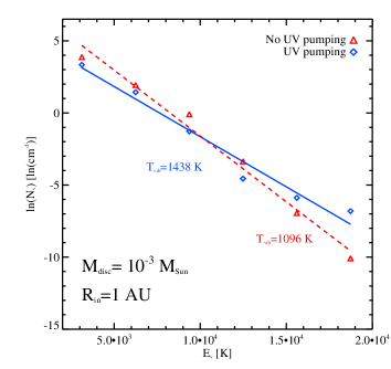
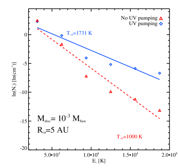
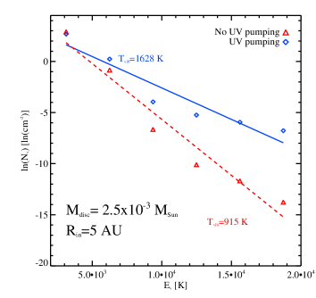
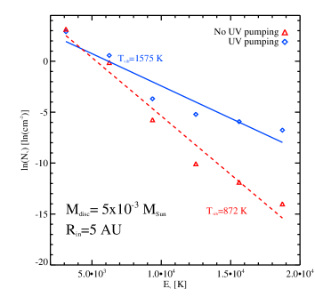
Figure 21: Similar to Fig. 20 but for models 5a, 5b to 8a, 8b. Among the models shown in this figure, the vibrational temperature differences between models with and without UV-pumping are the largest in the lowest mass disc with a inner hole (upper-right panel, model 6a with $M_{\mathrm{disc}}=10^{-3}$ M_⊙, $R_{\mathrm{disc}}$= 5 AU).

3.3 Results & Discussion

3.3.1 CO chemistry and location of the CO ro-vibrational emission

We focus on the CO chemistry of model 1a. The disc density, dust temperature, and gas temperature structures are shown in Fig. 10. The panels in Fig. 11 show the enhancement ($\chi$) with respect to the interstellar UV, the abundance relative to the total number of hydrogen-nuclei for He, electron, atomic hydrogen, molecular hydrogen, vibrationally excited H₂ (H2exc), C⁺, C, CO, CH₄, OH, and H₂O. The transition from C⁺ to C occurs at $\log$($\chi$/n) between -1 and -2, and the transition between C and CO occurs at $\log$($\chi$/n)$\sim$ -2.5 to -3.

In Fig. 12, we show the location of the CO $v=1-0$ $P$(19) and $v=4-3$ $P$(20) emissions overlaid with the number density of the three main collision partners (H, H₂, and electrons) for a 10^-2 M_⊙ disc model taking UV pumping or not into account (models 1a and 1b). Similar plots are displayed in Fig. 13 for models 3a and 3b. The CO lines are emitted up to a few AU after $R_{\mathrm{in}}$, where the density is high enough such that the level population is the closest to the LTE population for the fundamental transitions. The emitting area becomes more and more confined to the inner rim as the upper energy of the transition increases. In the 10^-2 M_⊙ disc model the fluxes are a few percents higher when UV pumping is switched on. The fundamental $P$(19) line is emitted in region where the gas is between 500 and 1000K. In the vertical direction, the CO ro-vibrational lines are mostly emitted in the disc region with $z/r$$\sim$0.2 and $R$$<$ 5 AU.

In the emitting region, the extinction in the visible $A_{\mathrm{V}}$ is below 1 and some H₂ molecules are excited by UV and/or hot enough to be vibrationally excited (the excited H₂ abundance reaches 10^-12-10^-9). As soon as it is formed, the warm or vibrationally excited H₂ reacts quickly with atomic oxygen to form OH. In turn, OH reacts with H₂ to form H₂O or with atomic carbon to form CO.

The OH and water vapour abundance are high for $z/r$$\sim$0.2 and $R$$<$ 5 AU. The central role played by OH in hot gas chemistry is discussed in model details in Thi & Bik (2005). The 1a and 1b disc models are massive enough such that in the inner disc midplane ($z/r<$0.1) the most abundant carbon-bearing gas-phase species are methane and C₂H₂ ($R$$<$ 3 AU), whereas most of the oxygen is locked in water vapour up to $R$$\sim$ 5 AU. The remnant oxygen is the form of atomic oxygen, CO, and other minor species. The gas in the inner disc is dense enough such that UV fluorescence is quenched by collisional de-excitations between the ro-vibrational levels.

3.3.2 CO Spectral Line Energy Distribution

The analysis of the CO ro-vibrational lines can be performed either by comparing directly the observed and modelled line fluxes or by using rotational diagrams. In Fig. 14 and 16 we plotted the continuum-subtracted line fluxes for model 1 to 4 (spectral line energy distribution, SLED) for the fundamental ($v$=1-0) and one “hot” transition ($v$=4-3). The shape of the SLEDs varies from model to model and between models with and without UV pumping. The large variety of the SLEDs illustrates the sensitivity of the CO ro-vibrational line fluxes to the disc parameters ($M_{\mathrm{disc}}$, $R_{\mathrm{in}}$, etc …). The line fluxes range from 10^-19 W m^-2 to a few 10^-16 W m^-2 for a low-mass disc (10^-4 M_⊙) with an inner hole to a few 10^-16 W m^-2 to for a massive disc (10^-2 M_⊙) at a distance of 140 pc. In comparison, we show in Fig. 15 the $v$=1-0 CO line fluxes (Brittain et al. 2003) for the massive disc AB Aur and the low-mass disc HD141569A.The observed fluxes from HD141569A should be scaled from its distance of 99 pc (van den Ancker et al. 1997) to 140 pc. Fluxes for the hot lines from the HD141569A disc are $\sim$ 10^-18 W m^-2 after scaling the fluxes to 140 pc. When UV pumping is included, the hot line fluxes from our models are of the order of 10^-19-10^-17 W m^-2. The shapes of the SLEDs for models with a small inner radius ($R_{\mathrm{in}}$= 1 AU, models 1 & 3) reflect the effects of highly optically thick lines. On the other hand, the shapes of SLEDS of models with a large inner radius ($R_{\mathrm{in}}$= 20 AU, models 2 and 4) are typical of optically thin or moderately optically thick lines. The observed line fluxes are best matched by models with a small inner radius whereas the shapes of the observed SLED are closer to models with a large inner radius. To obtain fluxes that are close to the observed values, the emitting gas should be close to the star, but at the same time lower surface densities are needed to have moderate optical depths for the CO lines. Interestingly, UV pumping will increase the line $v$=1-0 fluxes only by a factor of few and the $v$=4-3 fluxes by orders of magnitude. In our models, UV pumping does not dramatically change the shape of the SLEDS for $v=$1-0 and $v$=4-3 transitions.

We ran models with inclination from 1 to 89 degrees with the line ray-tracing module. The line fluxes vary by up to 30% for inclinations below 70 degrees. At high inclination, the cold CO in the outer flaring disc starts to reabsorb the emission from the inner disc.

3.3.3 CO ro-vibrational level excitation

The CO vibrational levels in the ground electronic state can be populated by collisions with the main chemical species (H, H₂, electrons, He), by formation pumping (i.e. formation of CO in an vibrationally excited level), by pumping by dust emission, or by UV-fluorescence pumping. The region of high warm CO abundance is H rich and H₂ poor (Kamp & Dullemond 2004) (see Fig. 12 and 13). We also plotted the excitation temperatures. We chose two typical transitions, one from the $v=1$ level and one from the $v=4$ level, to illustrate the efficiency of the excitation mechanisms. The relative population between the $v=1,J=19$ and $v=1,J=18$ and between $v=4,J=20$ and $v=4,J=19$ levels are shown as excitation temperatures in Fig. 17 and 18 for the high- and low-mass disc models, respectively. The excitation temperatures between the $v=1,J=19$ and $v=0$, $J=18$ levels in the line-emitting region are below the gas kinetic temperatures but higher than the radiation temperature at the line frequency 4.844 micron (subthermal population, see Fig. 24, 26 and 27 in the appendix). However, the excitation temperatures between the $v=4,J=20$ and $v=3,J=19$ levels are much higher than the gas kinetic and radiation (at 4.692 micron) temperatures (suprathermal population). We can distinguish between the excitation mechanisms of the $v=1$ level and that of the $v>1$ levels.

The $v=1$ level is mostly populated by collisions and IR pumping because the disc densities in those emitting regions are close to the critical densities (10¹⁰-10¹²cm^-3). The $v=1$ level population is weakly affected by UV-fluorescence pumping (see the upper panels of Fig. 17 and 18). Likewise the line fluxes for the fundamental transitions change by at most a factor four when UV-fluorescence pumping is taken into account (Fig. 14).

The collision rates with electrons are $\sim$ 100 times higher than with H but the electron abundance is $\sim$ 10^-6 lower than the H-atom abundance. The collision rates with He are of the order of 10^-16 cm³ s^-1 at 500 K. The abundance is 0.075 times less than H+H₂. Therefore He is not a major collision partner. The main collision partner in the CO ro-vibrational emitting region is atomic hydrogen, whose de-excitation collision rates with CO are two orders of magnitude (10^-12 cm³ s^-1 at 500 K) higher than rates with H₂.

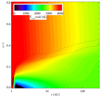
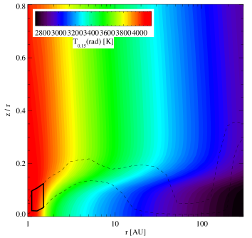
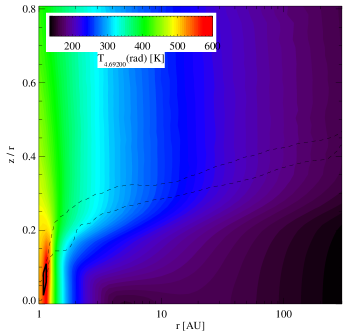
Figure 25: Radiation temperature $T_{\mathrm{rad}}$ at 0.15 micron and 4.692 micron for the $M_{\mathrm{disc}}=10^{-2}$ M_⊙, $R_{\mathrm{in}}$=1 AU disc models (left panel) and for the $M_{\mathrm{disc}}=10^{-4}$ M_⊙, $R_{\mathrm{in}}$=1 AU disc models (right panel). The black contours show the regions that emit 49% of the fluxes at 4.692 micron. The black dashed-line contours contain 70% of the fluxes in the vertical direction.

The $v>1$ levels have higher critical densities than the $v=1$ levels and require very high gas temperatures $T_{\mathrm{gas}}>$1000 K and high densities to be populated efficiently by collisions. Pumping of the $v>1$ levels by UV fluorescence becomes the prominent excitation mechanism. The excitation temperatures of UV-pumped levels (lower left-hand panels in Fig. 17 and 18) tend towards the effective radiation temperature (brightness temperature) in the UV (Fig. 25, the radiation temperatures at 0.15 micron).

The effect of UV pumping becomes more pronounced in the 10^-4 M_⊙ disc models (3a and 3b, Fig.13), where the gas densities and hence the UV-pumped high-$v$ level quenching efficiencies are lower and the UV photons are less absorbed by the dust grains (Fig. 25). In the $M_{\mathrm{disc}}$=10^-2 M_⊙ disc model, the UV pumping is confined to a very thin layer at the inner disc rim, whereas in the low-mass disc models ($M_{\mathrm{disc}}$=10^-4 M_⊙), the UV pumping occurs till $\sim$ 0.5 AU inside the disc because the UV photons can penetrate deeper in the disc.

The UV-fluorescence pumping can affect dramatically the line fluxes (Fig. 16). In particular the hot line $v=4-3$ $P$(20) is two orders of magnitude stronger with UV-pumping. The effect of UV pumping is better captured by computing the vibrational temperature (see Sect. 3.3.5). The relative rotational level populations within a vibrational level are less affected by UV pumping than the relative vibrational level populations (see the shape of the SLED in Fig. 14).

An alternative excitation mechanism is the formation pumping of CO. The CO formation reaction via C + OH has an exothermicity of -6.5 eV and a rate of $k_{\mathrm{chem}}\sim$10^-10 cm³ s^-1 (Zanchet et al. 2007). The excess energy is used to pump CO to high vibrational levels with a maximum population at $v$=10 (Bulut et al. 2011). The formation of CO constitutes a pumping mechanism for CO.

We can compare the efficiency of the chemical pumping with the efficiency of the population of the $v$=1 level by collisions with atomic hydrogen by noting that OH reaches a maximum abundance of $\sim$10^-6 (Fig. 11). The chemical pumping rate assuming atomic carbon abundance [C]$\sim$∼10^-4 is $k_{\mathrm{chem}}n_{\mathrm{C}}n_{\mathrm{OH}}\sim$ 10^-20 $n^{2}$ cm⁻³ s⁻¹ , where $n$ is the gas density. Collision rates with atomic hydrogen are of the order of 10${}^{-16}n^{2}$ cm⁻³ s⁻¹, a few orders of magnitude more efficient than the chemical pumping.

3.3.4 Rotational diagram for the fundamental transitions

The analysis of the line fluxes using a rotational diagram can provide more insight than the study of the shape of the SLEDs. We plotted in Fig. 19 the fundamental transition rotational diagram, i.e. the log of the level column density versus $B_{\mathrm{CO}}J^{\prime}(J^{\prime}+1)$, where $B_{\mathrm{CO}}$ is the rotational constant in Kelvins, for the 10^-2 and 10^-4 M_⊙ $R_{\mathrm{in}}$=1 AU and 20 AU models with (blue symbols) and without UV pumping (red symbols). The shape of a rotational diagram is affected by NLTE (subthermal population and IR/UV pumping) and optical depth effects. To obtain the optically thin emission in LTE (purple solid lines), we populated the CO ro-vibrational levels assuming $T_{\mathrm{ex}}=T_{\mathrm{gas}}$. The line fluxes were computed in the optically thin approximation, i.e. optically depth effects, which would have prevented the flux from increasing indefinitely, were not taken into account.

The optically thin CO LTE populations probe the actual kinetic temperatures in the discs. The populations were calculated by summing for each level all the CO molecules at that level in the models, assuming that the population is in LTE. For each model, the rotational population of the $v=1$ level can be relatively easily matched by a single temperature $T_{\mathrm{rot}}^{\mathrm{LTE}}$ because the CO fundamental lines probe a small region in discs where the gas is warm and dense. Moreover, the densities are high enough for the low- and medium-$J$ rotational levels within the $v=1$ level to be close in rotational LTE. The line profiles will be wider for high-$J$ than for low-$J$ transitions in discs not seen edge-on. The LTE temperatures (fits to the purple lines shown with black crosses) $T_{\mathrm{LTE}}$ are given in Table 4. The gas is warmer for lower mass, hence lower density discs because the molecules, which are efficient gas coolants, are more rapidly formed in dense gases.

Since the stellar radiation decreases with distance squared, it is normal that the gas is cooler for discs with an inner radius starting at 20 AU rather than at 1 AU. Since CO ro-vibrational lines are efficient coolant for the gas, the gas probed by the CO gas is warmer (i.e. with higher $T_{\mathrm{rot}}^{\mathrm{LTE}}$) when the number of ro-vibrational levels decreases (Table 4).

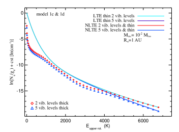
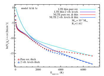
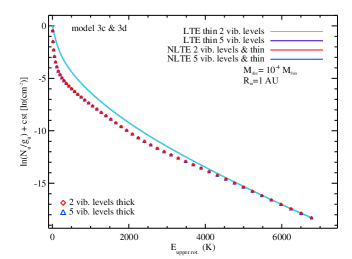
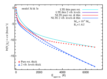
Figure 22: Disc CO $v=0$ rotational population at LTE and at NLTE for the $R_{\mathrm{in}}$=1 AU models with only the $v=0$, $v=1,2$, and $v=1,2,3,4,5$ levels taken into account. All populations have been normalized.

The red and blue lines in Fig. 19 correspond to the CO ro-vibrational NLTE level population computed locally in the disc using the 1+1D escape probability method. Those lines show that the level populations are rotationally subthermal. The effects are stronger for less massive (10^-4 M_⊙), hence less dense discs.

The ro-vibrational NLTE population is orders of magnitude smaller than the ro-vibrational LTE population for all models, pointing to a subthermal population of the excited ro-vibrational levels: the rotational level populations within a vibrational level can be in LTE, while the vibrational level populations are subthermal. Assuming a transition probability of 10 s^-1 and a rate coefficient of 10^-16 cm³ s^-1 (H₂) to 10^-12 cm³ s^-1 (H), the critical density is 10¹¹–10¹⁵ cm^-3. Such high densities are reached only close to the star in the inner disc midplane of massive discs.

Radiative transfer of the optically thick lines decreases further the populations derived from the analysis of rotational diagrams. One consequence is that rotational temperatures derived from fitting points from low-$J$ optically thick lines in rotational diagrams would appear lower than the actual gas kinetic temperatures. In appendix A.1, we provide a simple analytical method to analyse observations of optically thick ¹²CO v=1-0 emission lines. Optical thickness results in flux differences between lines of transitions that have the same upper level but lower levels that differ by $\Delta J$ and different transition probabilities: the $P$ ($J"=J^{\prime}+1$) and the $R$ ($J"=J^{\prime}-1$) branches. As expected, the column density differences between LTE and NLTE population are strong in models 1a and 1b and are weak in model 4a and 4b.

The $R$-branch transitions generally have higher transition probabilities (i.e. with higher Einstein-$A$ coefficients) than $P$-branch transitions. Hence, if the lines are optically thick, the column densities derived from $R$-branch lines are the smallest ($N_{J^{\prime}}\propto F_{\nu}/A_{ul}$ and $F_{\nu}$ are almost the same). Lines are optically thick up to very high $J$, giving rise to a steep slope for the low $J$ and to a shallow slope for the moderate $J$ lines (symbols). Observed rotational diagrams of Herbig Ae discs show similar shapes (Blake & Boogert 2004; Brittain et al. 2007; Brown et al. 2012). Only lines from $J^{\prime}>$ 40 ($>$ 25 for the 10^-4 M_⊙, $R_{\mathrm{in}}$=20 AU disc model) are optically thin: their populations join the optically thin NLTE populations and the differences between the $P$ and $R$ branch column densities fade away. The optical thickness of the lines and rotationally subthermal population of the levels can cause the lines to be actually optically thick but effectively thin, especially in discs where the continuum emission at 4-5 micron is optically thin.

UV pumping affects the level population for all levels with $v>1$ whatever the inner disc radius. The main effect of UV pumping is to populate the high-$J$ and $v>1$ (see discussion below and Fig. 20) levels at the expense of the lower $v=0,J$ levels. We also ran the models with UV pumping but without collision excitations between the ground and electronic excited states. However, we noticed no difference over a few percents.

The shape of the rotational diagrams (symbols) shows that it would be difficult to fit straight lines to estimate the excitation temperatures. Moreover, they do not reflect the actual CO population due to strong optical depth effects.

3.3.5 Vibrational temperature and UV/IR fluorescence pumping

The vibrational temperature measures the relative population of the vibrational levels. We plotted in Fig. 20 and 21 the log of the vibrational level population ($\ln(N_{v})$) as function of the vibration energy $E_{v}=3122v$, where $v$ is the vibrational quantum number (Brittain et al. 2007). The vibrational level population is the sum of all the rotational level populations at that vibrational level.

We derived the vibrational temperatures by fitting straight lines through the data in models with and without UV pumping (nine and five vibrational levels) apart from the 10^-2 M_⊙ $R_{\mathrm{in}}$=1 AU model where only $v$=4, 5, and 6 levels are taken into account because a straight line could not be fitted when those levels were included. The values are reported in the last column of Table 4.

Even without UV pumping, the vibrational temperatures are higher than the LTE rotational temperatures. However, the rotational temperatures derived using points in the shallow slope of the diagrams will yield temperatures higher than the LTE values and closer to the non-pumped vibrational temperatures.

Two clear trends can be seen from the vibrational diagrams and the temperatures in Table 4. First, the vibrational temperature is higher for the lower mass disc. Second, the vibrational temperature increases with the inner hole size if UV pumping is switched on, whereas it decreases if UV pumping is switched off.

When the UV pumping is not present, the high vibrational levels can be populated by collisions and/or by IR pumping. The collision rates for vibrational transitions are lower than for rotational transitions. If the vibrational levels are populated by collision only, then the vibrational temperatures should be lower then the rotational temperatures. Therefore, collisions play a minor role in populating the high-$v$ ro-vibrational levels, leaving IR pumping as the dominating mechanism. In the absence of UV pumping, the vibrational temperatures are still higher than the maximum dust temperatures in the discs (max($T_{\mathrm{dust}}$) in Table 4). The IR continuum flux between 1 and 5 $\mu$m is dominated by the dust emission for the models with $R_{\mathrm{in}}$=1 AU (models 1 and 3) and by the stellar emission for models with an inner hole ($R_{\mathrm{in}}$=20 AU; models 2 and 4). The vibrational temperatures are the same whether five or nine vibrational levels are taken into account in the models, suggesting that the effect of IR pumping does not depend on the vibrational level.

As the gas cools with increasing inner radius, the high-$v$ levels are less populated. Absorption of UV photons directly by CO molecules will favour the population of high-$v$ levels unless high gas densities quench the overpopulation. The gas density at the inner edge decreases with the edge’s distance to the star. Higher $R_{\mathrm{in}}$ values and lower mass discs will have less collisional de-excitations of UV-pumped high-$v$ levels.

3.3.6 Effect of IR pumping on the rotational population of the $v=$1 level

The left-hand panels in Fig. 22 show the differences between the case with two and five vibrational levels. For the massive disc with $M_{\mathrm{disc}}$=10^-2 M_⊙, the population decreases as more vibrational levels are included. The CO $v>$1 levels can be pumped by absorptions in the hot and overtone bands of stellar or dust IR photons, resulting in lower populations of the $v$=1, $J$ levels (upper right-hand panel). The pure rotational levels in LTE cannot be explained by a single excitation temperature contrary to the rotational levels in the first vibrational excited state. The pure rotational transitions probe much larger disc areas with wide-ranging physical conditions than do the fundamental ro-vibrational transitions. This stems from the low critical densities needed to populate the pure-rotational levels.

The right-hand panels in Fig. 22 compare the population in models where only rotational levels with $v=$0 are included and where the levels $v=$0 and $v=$1 are included. In the optically thin cases (solid lines), the differences between the cyan and blue lines reflect the rotationally subthermal populations for the high-$J$ populations. The low-$J$ levels are at LTE. However, the high optical depths for the low- and mid-$J$ lines result in lower derived population and the appearance of a change in the slope at $J$=8–12. At high $J$ ($E_{\mathrm{rot}}>$2000 K), the overpopulations when only the ground vibrational ($v$=0, $J$) are modelling artifacts because overlapping energies occur between the $v$=0, high-$J$ level energies and that of the $v$=1, low-$J$ levels. For a gas at temperature $T$, both the high $J$ and low $J$ of the $v=$1 levels can and should be populated. In warm and hot gases, models that do include the pure rotational levels only may overestimate their populations.

4 Conclusion

We have implemented a complete CO ro-vibrational molecular model in the ground $X^{1}\Sigma^{+}$ and $A^{1}\Pi$ electronic state in the radiative chemo-physical code ProDiMo. We gathered existing collisional rate coefficients and used scaling rules to extrapolate the missing ones. Collision rates of CO with atomic hydrogen are two orders of magnitude higher than rates with molecular hydrogen and three orders of magnitude higher than with He.

We ran models that include continuum, NLTE-line radiative transfer assuming a Voigt line profile, chemistry, and gas thermal balance to understand the effect of UV on the population of high-vibrational and high-rotational levels in protoplanetary discs. CO ro-vibrational lines are emitted within the first few AU and probe disc regions where CO is quickly formed via C + OH, with OH being formed via the fast reaction of vibrationally excited H₂ with atomic oxygen.

The amount of atomic hydrogen is high in the CO line-emitting region. The $v=1$ level population is dominated by collisional excitation with atomic hydrogen with contributions from IR-pumping and UV-fluorescence pumping. Excitation of high-$J$ and high-$v$ levels by UV and IR photons can be efficient, especially in low mass discs where collisional quenching is less rapid than in high-mass discs. The molecular gas is rotationally “cool” and subthermal but vibrationally “hot” and suprathermal. However, only the detection of hot lines ($v^{\prime}\geq$ 2, $\Delta v$=1) in discs can provide a test of the efficiency of UV-fluorescence.

The pure rotational transitions probe the entire disc while the ro-vibrational transitions probe the inner warm disc region. Therefore the rotational temperature depends on the vibrational number of the initial level. It is difficult to derive accurate temperatures and column densities from the optically thick ¹²CO fundamental emissions. Spatially and spectrally resolved CO, ¹³CO, C¹⁸O, and C¹⁷O ro-vibrational observations are needed to disentangle the optical depth effects and constrain the location of the line emissions. The low- and medium-$J$ rotational levels on the ground and first excited vibrational levels are populated in LTE in discs due to the low critical densities of the pure rotational transitions.

Future studies will focus on studying the effects of disc parameters (mass, size, flaring index, …) on the CO ro-vibrational emissions and will include larger numbers of vibration levels and electronic excited states.

Appendix A Appendix

A.1 Rotational diagram analysis for levels in LTE and optically thick lines

We adopted the rotational diagram analysis that takes optical depth effects into account (also called population diagram analysis in Goldsmith & Langer 1999). A similar approach was taken by Goto et al. (2011). The line intensity emitted by a slab at a single temperature reads

$$\log{I_{\nu}}=\log{\left(\tau_{\nu}B_{\nu}\right)}+\log{\left(\frac{1-e^{-\tau_{\nu}}}{\tau_{\nu}}\right)}.$$ (26)

$B_{\nu}$ is the Planck function at the excitation $T_{ex}$=$T_{rot}$=$T_{vib}$. The second term in the right-hand side is an optical depth correction factor to the optically thin rotational diagram. The term $\beta=(1-\exp{(-\tau_{\nu})})/\tau_{\nu}$ is akin to the escape probability. The maximum optical depth occurs at $E_{rot}\sim kT_{rot}$, where $E_{rot}$ is the rotational upper level energy of an emission line. In the Born-Oppenheimer approximation, $E_{u}=E_{rot}+E_{vib}$. The rotational energy for CO can be approximated by $E_{rot}=B_{rot}J_{u}(J_{u}+1)$, with the rotational constant $B_{rot}=$ 2.76 K. The maximum optical depth occurs when $J_{u}\simeq\sqrt{T_{rot}/B_{rot}}$. The line optical depth is

$$\tau_{\nu}=\left(\frac{c^{2}}{8\pi}\right)\left(\frac{A}{\nu^{3}}\right)\left(\frac{c}{\Delta v}\right)\left(e^{(h\nu/kT_{ex}}-1\right)x(T_{rot},T_{vib})N(\mathrm{CO})/\cos(i),$$ (27)

where $\nu$ is the line frequency, $A$ the Einstein spontaneous emission probability of the transition, $c$ the speed of light, $\Delta v$ the turbulent width, $N$(CO) the CO column density, $i$ the disc inclination, and

$$x(T_{rot},T_{vib})=\frac{e^{-E_{rot}/kT_{rot}}}{Q_{rot}}\times\frac{e^{-E_{vib}/kT_{vib}}}{Q_{vib}}$$ (28)

is the CO fractional population in the initial level ($v^{\prime}$,$J^{\prime}$). For CO, $Q_{rot}\simeq kT_{rot}/B_{\mathrm{C}O}+1/3$ ($B_{\mathrm{C}O}=2.76$ K) and $Q_{vib}=1/(1-\exp(-3122/T_{vib})$ are the rotational and vibrational partition function respectively (Brittain et al. 2007).

The rotational diagram of AB Aur (Fig. 23) shows three parts: a steep slope corresponding to increasing optical depth until $E_{rot}\sim kT_{ex}$, then a shallow slope where the line optical depth decreases because the higher the rotational level, the less they are populated. At very high $J$, the slope steepens again. This behaviour also appears in our theoretical rotational diagrams, but the second turning point occurs at higher $J$ than in the observations. The second slope change corresponds to lines with $\tau<$1. Assuming that the population is in LTE, we fitted the AB Aur rotational diagram by a model that takes the optical depth effects into account (Goldsmith & Langer 1999). The model parameters are the CO column density $N$(CO)=4.2 $\times$ 10¹⁷ cm^-2, the mean excitation temperature $T_{ex}\simeq$ 600 K (we assume that the vibrational temperature is equal to the rotational temperature), the turbulent width $\Delta v$=0.05, and the inclination $i$=30 degree. In the upper panel of Fig. 23, the analytical solid curve compares well with the observations. The dashed-line curve shows the same model where optical depth effects are not taken into account. The lower panel shows the derived optical depths, which reach $\sim$ 47.

A.2 Excitation, radiation, and gas kinetic temperatures

We define the radiation (brightness) temperature $T_{\mathrm{rad}}$ at a given wavelength as the equivalent blackbody temperature that will match the specific intensity computed by the continuum radiative transfer at a given location in the disc (Fig. 24 and 25). We also show temperature ratios in Fig. 26 and 27: the excitation over the radiation and the excitation over the gas kinetic temperatures.

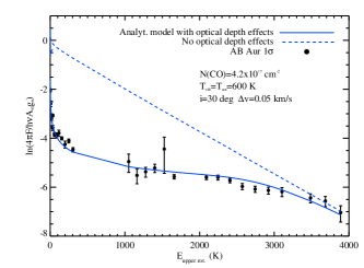
Figure 23: The upper panel shows the comparison between AB Aur and an analytical model rotational diagram for the ¹²CO $v$=1-0 transitions observed by Brittain et al. (2003). The solid blue line shows the fit by an analytical model that takes optical depths into account. The results from the same model but without the effect of optical depth are shown in dashed blue line. The lower panel shows the derived line optical depth.

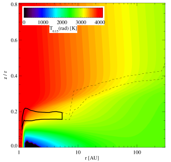
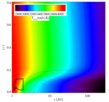
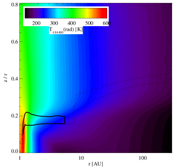
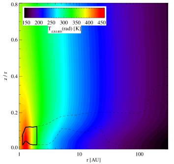
Figure 24: Radiation temperature $T_{\mathrm{rad}}$ at 0.15 micron and 4.844 micron for the $M_{\mathrm{disc}}=10^{-2}$ M_⊙, $R_{\mathrm{in}}$=1 AU disc models (left panel) and for the $M_{\mathrm{disc}}=10^{-4}$ M_⊙, $R_{\mathrm{in}}$=1 AU disc models (right panel). The black contour shows the regions that emit 49% of the fluxes at 4.844 micron. The black dashed-line contours contain 70% of the fluxes in the vertical direction.

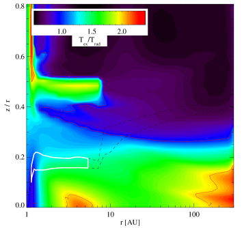
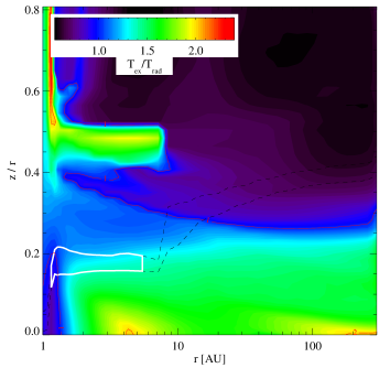
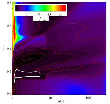
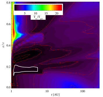
Figure 26: $T_{\mathrm{ex}}(v=1,J=19)/T_{\mathrm{rad}}(4.844)$ (upper panels) and $T_{\mathrm{ex}}(v=1,J=19)/T_{\mathrm{gas}}$ (lower panels) structures for the $M_{\mathrm{disc}}$=10^-2 M_⊙, $R_{\mathrm{in}}$=1 AU disc models. The left panels correspond to the model with UV pumping and the right panels to models without UV pumping. The contours are labelled in red. The white contours encompass the regions that emit 49% of the fluxes at 4.844 micron. The dashed-line contours contain 70% of the fluxes in the vertical direction.

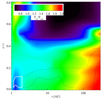
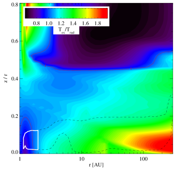
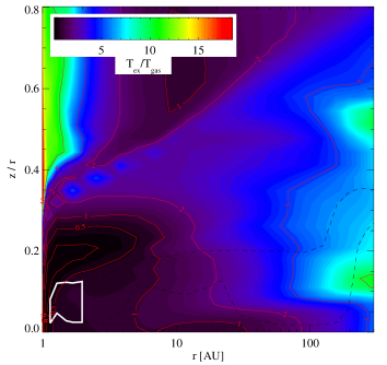
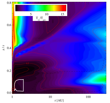
Figure 27: $T_{\mathrm{ex}}(v=1,J=19)/T_{\mathrm{rad}}(4.844)$ (upper panels) and $T_{\mathrm{ex}}(v=1,J=19)/T_{\mathrm{gas}}$ (lower panels) structures for the $M_{\mathrm{disc}}$=10^-4 M_⊙, $R_{\mathrm{in}}$=1 AU disc models. The left panels correspond to the model with UV pumping and the right panels to models without UV pumping. The contours are labelled in red. The white contours encompass the regions that emit 49% of the fluxes at 4.844 micron. The dashed-line contours contain 70% of the fluxes in the vertical direction.