Study of Loschmidt Echo for two-dimensional Kitaev model
Abstract
In this paper, we study the Loschmidt Echo (LE) of a two-dimensional Kitaev model residing on a honeycomb lattice which is chosen to be an environment that is coupled globally to a central spin. The decay of LE is highly influenced by the quantum criticality of the environmental spin model e.g., it shows a sharp dip close to the anisotropic quantum critical point (AQCP) of its phase diagram. The early time decay and the collapse and revival as a function of time at AQCP do also exhibit interesting scaling behavior with the system size which is verified numerically. It has also been observed that the LE stays vanishingly small throughout the gapless phase of the model. The above study has also been extended to the 1D Kitaev model i.e. when one of the interaction terms vanishes.
pacs:
05.50.+q,03.65.Ta,03.65.Yz,05.70.JkI Introduction
A quantum phase transition is a zero temperature transition of a quantum many body system driven by a non-commuting term of the quantum Hamiltonian which is associated with a diverging length as well as a diverging time scale sachdev99 ; chakrabarti96 . In recent years, a plethora of studies are being carried out which attempt to bridge a connection between quantum phase transition and quantum information theory nielsen00 ; vedral07 . For example, information theoritic measures like entanglement, quantum fidelity zanardi06 ; zhou08 ; gu10 ; gritsev10 , decoherence zurek91 ; haroche98 ; zurek03 ; joos03 and quantum discord sarandy09 ; dillenschneider08 , etc., are being studied close to the quantum critical point (QCP). These measures not only capture the singularities associated with the QCP but also show distinct scaling relations which characterizes it. There have also been numerous studies on decoherence (or loss of phase information) in a quantum critical system which is closely connected to the LE to be discussed in this work; understanding decoherence is essential for successful achievement of the quantum computation.
To study the LE in a quantum critical environment, we make resort to the central spin model zanardi in which a central spin is coupled globally to an environmental spin model (which in this case is the two dimensional Kitaev model). The LE (with the in some ground state ) is given by
Here the and are the two Hamiltonians with which the ground state evolves, where the term arises due to the coupling of the with the . It has been established that the LE shows a decay near the critical point of the with a decay rate that marks the universality associated with the QCP of zanardi ; zhang09 ; rossini07 ; sharma12 . Also the LE shows collapse and revival as a function of time when the is at the QCP.
The proposed work is organized in the following way: Sec.I presents the model Hamiltonian, the phase diagram and discussion about the AQCP. In sec.II, we describe the general calculation of the LE and in the subsequent subsections we study the scaling of the short time decay close to the AQCP and its collapse and revival with time.
II Model, Phase Diagram and Anisotropic Quantum Critical Point (AQCP)
The Hamiltonian of the Kitaev model on a honeycomb lattice is given by
| (1) |
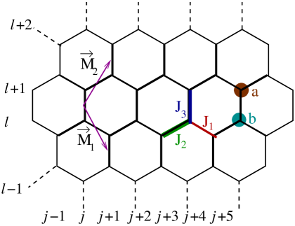
where and signify the column and row indices respectively of the honeycomb lattice while , and are coupling parameters for the three bonds (see Fig. (1)) kitaev06 ; sengupta08 ; and , are the Pauli spin matrices with (, and ), denoting the spin component.
We will assume the parameters , and are all positive and confine our analysis on the plane , since only the ratio of the coupling parameters appear in the subsequent calcuations. The most exciting property of this model is that even in two dimensions it can be exactly solved using Jordan-Wigner (JW) transformationlieb61 ; barouch70 ; kogut79 ; bunder99 ; kitaev06 ; chen ; feng in terms of Majorana fermions given by
| (2) |
Here, , , and are all Majorana fermion operators, they obey the relations and . One can now change the lattice site indices of honeycomb lattice to a 2-dimensional vector , where which labels the midpoints of the vertical bonds of the honeycomb lattice. Here and take all integer values so that the vectors form a triangular lattice. The Majorana fermions and are placed at the top and bottom sites respectively of the bond labeled by . The whole lattice is spanned by the vectors and , see Fig. (1).
Under the transformation to Majorana fermions as defined in Eqs. (2), Hamiltonian (1) takes the form
| (3) |
where =. These operators have eigenvalues independently for each and commute with each other and also with which makes the Kitaev model exactly solvable. Since is a constant of motion one can use one of the eigenvalues for each in the Hamiltonian. The ground state of the model corresponds to kitaev06 . With , we can easily diagonalize the Hamiltonian (3) quadratic in Majorana fermions.
The Fourier transform of the Majorana fermions can be defined as
| (4) |
similarly also has same Fourier transform relation. The ’s and ’s are Dirac fermions which follow the fermionic anti-commutation relations. Here, is the total number of sites and is the number of unit cells. In the above sum given in Eq. (4), is extended over half of the Brillouin zone of the hexagonal lattice due to Majorana nature of the fermions sengupta08 . We recall that the full Brillouin zone on the reciprocal lattice represents a rhombus with vertices = and . In the momentum space the Hamiltonian (3) takes the form where and the reduced Hamiltonian , can be expressed in terms of Pauli matrices as
| where | |||||
| and | (5) |
The eigenenergies of the are given by
| (6) |
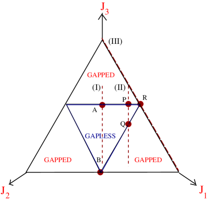
This energy spectrum corresponds to two energy bands; it is noteworthy that for , the band gap vanishes for some particular modes leading to the gapless phase of the Kitaev model. The phase diagram of the model is shown in an equilateral triangle satisfying the relation and (see Fig. (2)); one can easily show that the whole phase is divided into three gapped phases, separated by a gapless phase (inner equilateral triangle) which is bounded by gapless critical lines , and .
On the critical line energy gap goes to zero for the four modes given by = and which are the four corner points of Brillouin zone. One can now expand and around one of the critical modes for , in the form
| (7) |
where and are the deviations from the above mentioned critical modes. We note that varies linearly and varies quadratically in and . The point (where ) denoted by A in (Fig. (2)) needs to be checked carefully. This is an AQCP hikichi with energy dispersion along () and along (). The corresponding dynamical exponents are given by and , respectively.
For , is also an AQCP that can be shown using a rotation to a new coordinate system
| (8) |
in which and take the form
| (9) |
where , , and . Therefore, for a general AQCP the dispersion will vary linearly and quadratically along and directions, respectively, with two dynamical exponents and .
III Qubit Coupled To Term Of the Kitaev Hamiltonian
In this section we will provide a general calculation of the LE considering Kitaev model on a honeycomb lattice as an environment () that is coupled to a central spin- (). We shall denote the ground state and excited state of the central spin by and respectively. is coupled to term of Hamiltonian only when the central spin is in the excited state . Therefore the composite Hamiltonian takes the form
| (10) | |||||
where is the coupling strength of to . We shall work in the limit of .
We consider that the is initially in a generalized state (with the coefficients satisfying the condition ), and the is initially in the ground state . The evolution of the environmental spin model splits into two branches, given by and ; the evolution of is driven by the Hamiltonian (when the is in the ground state and hence there is no term present in the Hamiltonian), whereas evolves with , where , is the effective potential arising due to the coupling between and . The wave function of the composite system at a time is given by
| (11) |
As a result the LE is given by
| (12) | |||||
Here, we have exploited the fact that the is an eigenstate of the Hamiltonian .
Following Fourier transformation and Bogoliubov transformation the diagonalized form of the Hamiltonian (1) is given by
| (13) |
where the ’s and ’s are Bogoliubov fermionic operators defined as
| with | (14) |
and the energy spectrum is given by (see Eqs.(5) and (6))
| (15) |
where and are defined in Eq.(5), and corresponds to the value with instead of .
The complete ground state of can be written in the form (see Ref. [victor12, ] for details),
| (16) |
where runs over half of the Brillouin zone of the hexagonal lattice. Following mathematical steps identical to those in [zanardi, ; sharma12, ], it can be shown that Eq.(16) leads to the expression for the LE given by
| (17) |
where, and . The expression for LE closely resembles that of the case when the transverse Ising chain is chosen to be the environment zanardi . For numerical analysis of Eq.(17), we shall use and in terms of two independent variables and , with . The and are given by sengupta08
| (18) |
which span the rhombus uniformly. Avoiding the corner points of the Brillouin zone ( where the LE results in a zero value), we vary and from to in steps of , where is the system size victor12 and consider only the half of the Brillouin zone using the condition .
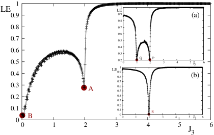
The LE is calculated numerically as a function of using Eq.(17) and it shows dip at all critical points. To illustrate this, we choose three paths along which the interaction is varied. In the first case is varied along the path (path ‘I’ in Fig. (2)) so that the model enters from the gapped phase to the gapless phase (extending in the region ) crossing the AQCP (point ‘A’ in Fig. (2)) at . The LE shows a sharp dip at point A and there is a revival with a small magnitude which again decays at the end point B, (see Fig. (3)). Now surprising result shows up when the path is so chosen (path ‘II’ in Fig. (2), given by the equation ) that the system enters the gapless phase through an AQCP with , (denoted by ‘P’ in Fig. (2)). The LE shows a sharp dip at the point P and stays close to its minimum value (with a small revival as observed in path I) throughout the gapless phase and again shows a rise when the system exits the gapless phase through the point Q. In contrary, for the case when is changed along the line , (path ‘III’ in Fig. (2)), one observes only a single drop in the LE near (see Fig. (3), inset (b)); this is associated with the critical point of the one-dimensional Kitaev model. In the next section we will study the scaling of the short time behaviour of LE close to these critical points and the collapse and reviaval of LE with time when the is right at the critical point.
III.1 Path I: Anisotropic Quantum Critical Point ()
As discussed in Sec.II, is an AQCP with critical exponents along direction and along direction. At this point energy gap vanishes for the three critical modes given by and in half of the Brillouin zone. Now we will study the short time behavior of the LE (in Eq. (17)) close to the AQCP. We define a cutoff frequency such that modes up to this cut-off only are considered to calculate the decay of LE at short time close to the AQCP. Then the LE is given by
| (19) |
We define the quantity , such that . Expanding around one of the critical mode upto the cut-off, we get and therefore we obtain,
| (20) |
where = and is a integer nearest to . We therefore find an exponential decay of the LE in the early time limit given by
| (21) |
where . The anisotropic nature of the quantum critical point is reflected in the fact that scales as and is independent of . Further using the expression of , one can easily observe that it is invariant under the transformation and , where is some integer.
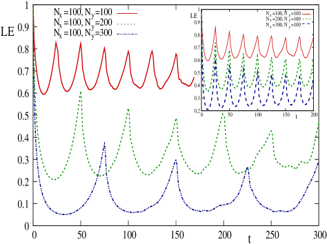
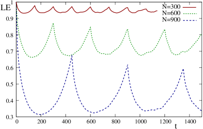
Now we fix and (point ‘A’ in Fig. (2)) and observe collapse and revival of LE with time (presented in the Fig. (4)). The time period of collapse and revival is proportional to , and is unaffected by the changes in ; this confirms the scaling result of the decay rate for the short time limit near the AQCP discussed above.
III.2 Path II: Anisotropic Quantum Critical Point
It has been shown that the point P in Fig. (2) (, ) is an AQCP which can be seen by choosing directions (see Sec II) and , perpendicular to victor12 . The critical exponents associated with this critical point are given by , and along and directions, respectively. To calculate the early time scaling in a similar spirit as in the previous section, we expand Eq. (17) near one of the critical modes up to the cut-off to obtain and . In the short time limit, the LE becomes
| (22) |
where, , and is an integer nearest to .
In fact comparing with the previous section III.1, one can see that in this case (instead of ) appears in the expression of the LE in the short-time limit. Further, from Eq. (22) and the expression of one observes that is invariant under the transformation and , with being some integer which is also observed in the collapse and revival behavior (see Fig. (5)).
III.3 Path III: One-dimensional Quantum Critical Point
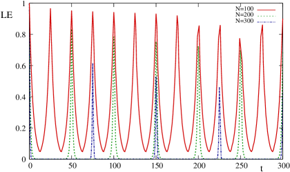
As mentioned already, along the line , (), the two dimensional spin model reduces to an equivalent one dimensional spin chain with energy gap vanishing at for and the corresponding dynamical exponent being . We shall now expand and around the critical mode to analyze the short time decay of LE, resulting into and . The LE hence takes the from
| (23) |
IV Conclusion
In this paper we study a variant of the central spin model in which a central spin (qubit) is globally coupled to an environment which is chosen to be a two-dimensional Kitaev model on a honeycomb lattice through the interaction term . Using the exact solvability of the Kitaev model, we have derived an exact expression of the LE when the interaction is varied in a way such that the system enters the gapless phase crossing the AQCP of the phase diagram. However, the behavior of the LE as a function of depends upon the path along which is varied. In the case when the AQCP, Q (with see Fig. (2)) is crossed, one observes a complete revival of the echo when the system exits the gapless phase to re-enter the gapped phase; this is in contrast to the case . For the case of there is only one sharp dip at the critical point which is associated with the QCP of the one-dimensional Kitaev model.
The early time scaling behavior for both the paths I and II close to the AQCP bear the signature of the fact that the gapless phase is entered crossing an AQCP with different exponents along different spatial directions. This is also confirmed by studying the collapse and the revival of the LE as a function of time. However, one does not observe a perfect collapse and revival (except for the equivalent one dimensional case); this may be because of the proximity to a gapless phase. The quasi-period of collapse and revival in all cases scale with the system size as . The case with reflects the fact that the system is essentially one-dimensional in this limit. It is straightforward to relate these results to the decoherence of the central spin close to a critical point.
This study of LE can be verified experimentally as presented by Zhang zhang09 ; they measure the LE as an indicator of quantum criticality for a one-dimensional quantum Ising model with an antiferromagnetic interaction using NMR quantum simulators. In this experiment, they prepare the ground state of the Hamiltonian (using the gate sequences) which need not be the true ground state but could be a state that approximates the ground state of the system well, and then measure the LE for finite number of spins. Similar experiments can be realized with the approximate ground state of the Kitaev model. Also, since the Kitaev model can also be realized using an optical latticeduan03 ; sen08 (where the couplings can be separately tuned with the help of different microwave radiations), there exists a possibility of verifying these results in an optical lattice also.
It should be noted that in a recent work, Pollmann pollmann10 , have studied the problem of the LE in a transverse Ising spin chain in the presence of a longitudinal field; more precisely they calculated the magnitude of the overlap between the final state reached following a slow quench across the QCP and its time evolved counterpart at time (generated following the time evolution with the final Hamiltonian). They observe a cusp-like minimum in the echo as a function of time in the limit when the spin chain is integrable. However, this behavior is smeared in the non-integrable case (with non-zero longitudinal field) thus providing a probe for integrable versus non-integrable behavior. In the present paper, we however deal with an equilibrium situation in which the spin chain is not quenched across the QCP, and observe the collapse and revival only at the QCP.
Acknowledgements
We acknowledge Amit Dutta, Victor Mukherjee and Aavishkar Patel for helpful discussions and comments. AR acknowledges B. K. Chakrabarti for valuable discussions and thanks IIT Kanpur for financial support during this work. SS thanks CSIR, New Delhi for Junior Research Fellowship.
References
- (1) S.Sachdev Quantum Phase Transitions(Cambridge University Press, Cambridge, England, 1999.)
- (2) B. K. Chakrabarti, A. Dutta and P. Sen, Quantum Ising Phases and transitions in transverse Ising Models, m41 (Springer, heidelberg, 1996).
- (3) M. A. Nielsen and I. L. Chuang, Quantum Computation and Quantum Information(Cambridge University Press, Cambridge, UK, 2000).
- (4) V. Vedral, Introduction to Quantum Information Science(Oxford University Press, Oxford, UK, 2007).
- (5) P. Zanardi and N. Paunkovic, Phys. Rev. E 74, 031123 (2006).
- (6) H. -Q. Zhou and J. P. Barjaktarevic, J. Phys. A: Math. Theor. 41, 412001 (2008).
- (7) S. J. Gu, Int. J. Mod. Phys. B 24, 4371 (2010).
- (8) V. Gritsev, and A. Polkovnikov, in Developments in Quantum Phase Transitions, edited by L. D. Carr (Taylor and Francis, Boca Raton) (2010).
- (9) W. H. Zurek, Phys. Today 44, 36 (1991).
- (10) S. Haroche, Phys. Today 51 36 (1998).
- (11) W. H. Zurek, Rev. Mod. Phys. 75 715 (2003).
- (12) E. Joos, H. D. Zeh, C. Keifer, D. Giulliani, J. Kupsch and I. -O. Statatescu, Decoherence and appearance of a classical world in a quantum theory (Springer Press, Berlin) (2003).
- (13) M. S. Sarandy, Phys. Rev. A 80, 022108 (2009).
- (14) R. Dillenschneider Phys. Rev. B 78, 224413 (2008).
- (15) H.T. Quan, Z. Song, X.F. Liu, P. Zanardi, and C.P. Sun, Phys.Rev.Lett. 96, 140604 (2006).
- (16) J. Zhang, F. M. Cucchietti, C. M. Chandrasekhar, M. Laforest, C. A. Ryan, M. Ditty, A. Hubbard, J. K. Gamble and R. Laflamme, Phys. Rev. A 79, 012305 (2009).
- (17) D. Rossini, T. Calarco, V. Giovannetti, S. Montangero and R. Fazio, Phys. Rev. A 75, 032333 (2007).
- (18) S. Sharma, Victor Mukherjee and Amit Dutta, Eur. Phys. J B 85, 143(2012).
- (19) A. Kitaev, Ann. Phys. (N.Y.) 321, 2 (2006).
- (20) K. Sengupta, D. Sen, and S. Mondal, Phys.Rev.Lett.100, 077204(2008); S. Mondal, D. Sen, and K. Sengupta, Phys.Rev.B78, 045101(2008).
- (21) E. Lieb, T. Schultz, and D. Mattis, Ann. Phys.(N.Y.) 16 37004 (1961).
- (22) E. Barouch, B. M. McCoy and M. Dresden, Phys. Rev. A. 2, 1075, (1970); E. Barouch and B. M. McCoy, Phys. Rev. A 3, 786 (1971).
- (23) J. B. Kogut, Rev. Mod. Phys. 51 659 (1979).
- (24) J.E. Bunder and R. H. McKenzie, Phys. Rev. B. 60, 344, (1999).
- (25) H.-D.Chen and Z. Nussinov, J.Phys.A41, 075001 (2008).
- (26) X.Y. Feng, G.M. Zhang, and T. Xiang, Phys. Rev. Lett. 98, 087204 (2007).
- (27) T. Hikichi, S. Suzuki, and K. Sengupta, Phys.Rev.B 82, 174305 (2010).
- (28) Victor Mukherjee, Amit Dutta, Diptiman Sen, Phys. Rev. B 85, 024301 (2012).
- (29) B. Damski, H.T. Quan and W.H. Zurek, Phys.Rev.A 83, 062104 (2011).
- (30) L. M. Duan, E. Demler, and M.D. Lukin, Phys. Rev. Lett. 91, 090402 (2003); A. Micheli, G.k. Brennen, and P. Zoller, Nature Phys. 2, 341 (2006).
- (31) D. Sen, K.Sengupta and S. Mondal, Phys. Rev. Lett. 101, 016806 (2008).
- (32) F. Pollmann, S. Mukherjee, A. G. Green, and J.E. Moore, Phys. Rev. E 81, 020101(R) (2010).