Finding Efficient Region in The Plane with Line segments

Abstract

Let $\mathscr{O}$ be a set of $n$ disjoint obstacles in $\mathbb{R}^{2}$, $\mathscr{M}$ be a moving object. Let $s$ and $l$ denote the starting point and maximum path length of the moving object $\mathscr{M}$, respectively. Given a point $p$ in ${R}^{2}$, we say the point $p$ is achievable for $\mathscr{M}$ such that $\pi(s,p)\leq l$, where $\pi(\cdot)$ denotes the shortest path length in the presence of obstacles. One is to find a region $\mathscr{R}$ such that, for any point $p\in\mathbb{R}^{2}$, if it is achievable for $\mathscr{M}$, then $p\in\mathscr{R}$; otherwise, $p\notin\mathscr{R}$. In this paper, we restrict our attention to the case of line-segment obstacles. To tackle this problem, we develop three algorithms. We first present a simpler-version algorithm for the sake of intuition. Its basic idea is to reduce our problem to computing the union of a set of circular visibility regions (CVRs). This algorithm takes $O(n^{3})$ time. By analysing its dominant steps, we break through its bottleneck by using the short path map (SPM) technique to obtain those circles (unavailable beforehand), yielding an $O(n^{2}\log n)$ algorithm. Owing to the finding above, the third algorithm also uses the SPM technique. It however, does not continue to construct the CVRs. Instead, it directly traverses each region of the SPM to trace the boundaries, the final algorithm obtains $O(n\log n)$ complexity.

I Introduction

Suppose there are a set ${\mathscr{O}}$ of $n$ disjoint obstacles and a moving object $\mathscr{M}$ in $\mathbb{R}^{2}$, and suppose $\mathscr{M}$ freely moves in $\mathbb{R}^{2}$ except that it cannot be allowed to directly pass through any obstacle $o\in\mathscr{O}$. See the right figure for example. The black line-segments denote the set of obstacles, and the black dot denotes the starting point of $\mathscr{M}$, the grey line-segment denotes the maximum path length that $\mathscr{M}$ is allowed to travel. We address the problem, how to find a region $\mathscr{R}$ such that, for any point $p$ if $\mathscr{M}$ can reach it, then $p\in\mathscr{R}$; otherwise, $p\notin\mathscr{R}$. (See Section 2 for more formal definitions and other constraint conditions.)

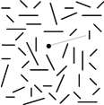
Figure 1: Example of Finding Achievable Region

Clearly, if there is no obstacle in $\mathbb{R}^{2}$, the answer is a circle, denoted by $C(s,l)$, where $s$ and $l$ denote the center and radius of the circle, respectively. Now consider the case of one obstacle as shown in Figure 2(a). Firstly, we can easily know any point in the region bounded by the solid lines is achievable for $\mathscr{M}$, without the need of making a turn, see Figure 2(b). Secondly, we can also easily know any point in the circle ${C}(a,dist(a,v_{1}))$ is achievable for $\mathscr{M}$, where $dist(\cdot)$ denotes the Euclidean distance, see Figure 2(c). Similarly, we can get another circle ${C}(b,dist(b,v_{2}))$, see Figure 2(d). Naturally, we can get the answer by merging the three regions, i.e., two circles and a circular-arc polygon.

By investigating the simplest case, we seemingly can derive a rough solution called RS as follows. Firstly, we obtain the region denoted by ${\mathscr{R}}_{d}$ in which any point is achievable for $\mathscr{M}$, without the need of making a turn. Second, for each vertex (or endpoint) $v$ of obstacles, if $\pi(s,v)<l$, we obtain the circle centered at $v$ and with the radius $l-\pi(s,v)$, where $\pi(\cdot)$ denotes the shortest path length in the presence of obstacles. Finally, we merge all the regions obtained in the previous two steps. Is it really so simple? (See Section II for a more detailed analysis.)

(a)

(b)

(c)

(d)

Figure 2: The simplest case. The black dot $s$ and solid line $\overline{ab}$ denote the starting point of $\mathscr{M}$ and the obstacle, respectively.

Motivations

Our study is motivated by the increasing popularity of location-based service [29, 32] and probabilistic answer on uncertain data [28, 1]. Nowadays, many mobile devices, such as cell phones, PDAs, taxies are equipped with GPS. It is common for the service provider to keep track of the user’ s location, and provide many location-based services, for instance finding the taxies being located in a query range, finding the nearest supermarkets or ATMs, etc. The database sever, however, is often impossible to contain the total status of an entity, due to the limited network bandwidth and limited battery power of the mobile devices. This implies that the current location of an entity is uncertain before obtaining the next specific location. In this case, it is meaningful to use a closed region to represent the possible location of an entity [6, 34]. In database community, they usually assumed this region is available beforehand, which is impractical. A proper manner to obtain such a region is generally based on the following information: geographical information around the entity, say ${G_{I}}$, the (maximum) speed of the entity, say $V_{M}$, and the elapsed time, say $T_{E}$. By substituting “$V_{M}\cdot T_{E}$” with the maximum path length $l$, ${G_{I}}$ with obstacles $\mathscr{O}$, it corresponds to our problem.

Our problem also finds applications in the so-called moving target search [19, 36]. Traditionally, moving target search is the problem where a hunter has to catch a moving target, and they assumed the hunter always knows the current position of the moving target [36]. In many scenarios (e.g., when the power of GPS - equipped with the moving target- is used up, or in a sensor network environment, when the moving target walked out of the scope of being minitored), it is possible that the current position of the moving target cannot be obtained. In this case, we can infer the available region based on some available knowledge such as the geographical information and the previous location. The available region here can contribute to the reduction of search range.

Related work

Although our problem is easily stated and can find many applications, to date, we are not aware of any published result. Our problem is generally falls in the realm of computational geometry. In this community, the problem of computing the visibility polygon (VP, a.k.a., visibility region) [14, 2, 37] is the most similar to our problem. Given a point $p$ and a set of obstacles in a plane, this problem is to find a region in which each point is visible from $p$. There are three major differences between our problem and the VP problem: (i) our problem has an extra constraint, i.e., the maximum path length $l$, whereas the VP problem does not involve this concept; (ii) in the VP problem, the region behind the obstacle must not be visible, whereas in our problem it may be achievable by making a turn; and (iii) the VP problem does not involve the circular arc segments, whereas in our problem we have to handle a number of circular arc segments. It is easy to see that our problem is more complicated.

We note that the Euclidean shortest path problem [21, 18, 3, 33, 23, 17, 31, 35] also involves the obstacles and the path length. In these two aspects it is similar to our problem. Given two points $p$ and $p^{*}$, and a set of obstacles in a plane, this problem is to find the shortest path between $p$ and $p^{*}$ that does not intersect with any of the obstacles. It is different from our problem in three points at least: (i) this problem is to find a path, whereas our problem is to find a region; (ii) the starting point and ending point are known beforehand in this problem, whereas the ending point in our problem is unknown beforehand; and (iii) the shortest path length is unknown beforehand in this problem, whereas the maximum path length $l$ in our problem is given beforehand.

Finally, our problem shares at least a common aspect(s) with other visibility problems [38, 20, 30, 9, 26, 27, 16] in this community, since they all involve the concept of obstacles. But they are more or less different from our problem. The art gallery problem [20] for example is to find a minimum set $\mathscr{S}$ of points such that for any point $q$ in a simple polygon $\mathscr{P}$, there is at least a point $p\in\mathscr{S}$ such that the segment $\overline{pq}$ does not pass through any edge of $\mathscr{P}$. The edges of $\mathscr{P}$ here correspond to the obstacles. The differences between this problem and our problem is obvious since our problem is to find a region rather than a minimum set of points. More details about the visibility problems please refer to the textbooks, e.g., [11, 8].

Our contributions

We formulate the problem — finding achievable region, offer insights into its nature, and develop multiple algorithms to tackle it.

Specifically, in Section 3, we present a simpler-version algorithm for the sake of intuition. The basic idea of this algorithm is to reduce our problem to computing the union of a set of circular visibility regions (CVRs), defined in Section II. Intuitively, the CVR can be obtained by computing a boolean union of the visibility region and the circle. The visibility region however, may not be always bounded, which leads to some troubles and makes this straightforward idea to be difficult to develop. We adopt a different way to compute the CVR instead of directly solving those troubles. Specifically, we first prune some unrelated obstacles based on a simple but efficient pruning mechanism that ensures all candidate obstacles to be located in the circle, which can simplify the subsequent computation. After this, we use the idea of the rotational plane sweep to construct the CVR, whose boundaries are represented as a series of vertexes and appendix points (defined in Section II) that are stored using a double linked list. We note that, for most CVRs, the circles used to construct them are unavailable beforehand. We use the visibility graph technique to obtain the circle. Once we obtain a new CVR, we merge it with the previous one. In this way, we finally get our wanted answer, i.e., the achievable region $\mathscr{R}$. This algorithm takes $O(n^{3})$ time.

We analyse the dominant steps of the first algorithm, and break through its bottleneck by incorporating the short path map (SPM) technique. Specifically, in Section 4, we show the SPM technique, previously used to answer the short path queries among polygonal obstacles, can be equivalently applied to the context of our concern. We use this technique to obtain those circles (that are used to construct most CVRs). Obtaining each circle needs $O(n^{2})$ time in the first algorithm, it takes (only) $O(\log n)$ time by using the SPM technique. This improvement immediately yields an $O(n^{2}\log n)$ algorithm.

Thanking the realization in Section 4 — the SPM technique can be used to the context of our concern, the third algorithm presented in Section 5 also uses this technique. It however, does not continue to construct the CVRs. Instead, it directly traverse each region of the SPM to trace the boundaries. By doing so, it gets a circular kernel-region and many circular ordinary regions. (Some circular ordinary regions possibly consist of not only circular arc and straight line segments but also hyperbolas, hence, sometimes we call them conic polygons.) Any two of these regions actually have no duplicate region, defined in Section II. In theory, we can directly output these conic polygons. We should note that Section II emphasizes a constraint condition — the output of the algorithm to be developed is the well-organized boundaries of the achievable region $\mathscr{R}$. In order to satisfy such a constraint, we only need to execute a simple boolean set operation (i.e., arrange all edges (segments) of these conic polygons and then combine them in order). Due to the SPM has complexity $O(n)$, naturally, the number of edges of all these conic polygons has the linear-size complexity. Moreover, in the context of our concern, the number of intersections among all these segments is clearly no more than $O(n)$, and constructing the SPM can be done in $O(n\log n)$ time (which has been stated in Section IV), all these facts form our final algorithm, obtaining an $O(n\log n)$ worst case upper bound.

We remark that although this paper focuses on the case of line-segment obstacles, the FAR problem in the case of polygonal obstacles should be easily solved using anyone of the above algorithms (maybe some minor modifications are needed).

Paper organization

In the next section, we formulate our problem, define some notations, and analyse the so-called rough solution mentioned before. Section III presents a simpler-version $O(n^{3})$ algorithm for the sake of intuition. Section IV presents a modified-version $O(n^{2}\log n)$ algorithm, and Section V presents our final algorithm, running in $O(n\log n)$ time. Finally, Section VI concludes this paper with several open problems.

II Preliminaries

II-A Problem definition and notations

Let $\mathscr{M}$ be a moving object in $\mathbb{R}^{2}$, we assume $\mathscr{M}$ can be regarded as a point compared to the total space. Let $\mathscr{O}$ be a set of $n$ disjoint obstacles in $\mathbb{R}^{2}$. We assume that the moving object $\mathscr{M}$ can freely move in $\mathbb{R}^{2}$, but cannot directly pass through any obstacle $o\in\mathscr{O}$. For clarity, we use $\mathbb{R}^{2}/\mathscr{O}$ to denote the free space. Let $s$ be the starting point of the moving object $\mathscr{M}$. (Sometimes we also call it the source point.) Given a point $p\in\mathbb{R}^{2}/\mathscr{O}$, assume that the moving object $\mathscr{M}$ freely moves from $s$ to $p$, the total travelled-distance of $\mathscr{M}$ is called the path length. We remark that, if $s$ and $p$ are identical in $\mathbb{R}^{2}$, the path length is not definitely equal to 0. The maximum value of path length that $\mathscr{M}$ is allowed to travel is called the maximum path length.

We use $l$ to denote the maximum path length of the moving object $\mathscr{M}$. Given two points $p$ and $p^{\prime}$ in $\mathbb{R}^{2}$, we use $\pi(p,p^{\prime})$ to denote the shortest path length in presence of obstacles (a.k.a., the geodesic distance). When two points $p$ and $p^{\prime}$ are to be visible to each other, we use $dist(p,p^{\prime})$ to denote the Euclidean distance between them. Given a point $p$ in $\mathbb{R}^{2}$, we say $\mathscr{M}$ can reach the point $p$ such that $\pi(s,p)\leq l$. (Sometimes, we also say $p$ is achievable for $\mathscr{M}$.) Given two closed regions, we say they have the duplicate region if the area of their intersection set does not equal to 0; otherwise, we say they have no duplicate region.

Definition II.1 (Finding achievable region).

The problem of finding achievable region (FAR) is to find a region denoted by $\mathscr{R}$ such that for any point $p$ in ${\mathbb{R}}^{2}$, if $\mathscr{M}$ can reach $p$, then $p\in\mathscr{R}$; otherwise, $p\notin\mathscr{R}$.

Clearly, the line segment is the basic element in geometries. This paper restricts the attention to the case of disjoint line-segment obstacles. (We remark that the case of polygonal obstacles should be easily solved using our proposed algorithms.) In particular, we emphasize that the output of the algorithm to be developed is the well-organized boundaries of the achievable region $\mathscr{R}$, rather than a set of out-of-order segments. Furthermore, we are interested in developing the exact algorithms rather than approximate algorithms. Unless stated otherwise, the term obstacles refers to line-segment obstacles in the rest of the paper.

Let $\mathscr{E}$ be the set of all endpoints of obstacles $\mathscr{O}$, we use $\mathscr{E}^{\prime}$ to denote the set of endpoints such that (i) for each endpoint $e\in\mathscr{E}^{\prime}$, $\pi(s,e)<l$; and (ii) for each endpoint $e\in\mathscr{E}$ but $e\notin\mathscr{E}^{\prime}$, $\pi(s,e)\geq l$. For clarity, we call the set $\mathscr{E}^{\prime}$ the effective endpoint set. (Sometimes we call the endpoint $e\in\mathscr{E}^{\prime}$ the effective endpoint.) Given any set, we use the notation “$|\cdot|$” to denote the cardinality of the set (e.g., $|\mathscr{E}^{\prime}|$ denotes the number of effective endpoints). Given two points $p$ and $p^{\prime}$, we use $\overline{pp^{\prime}}$ to denote the straight line segment joining the two points. Given a circular arc segment with two endpoints $p$ and $p^{\prime}$, we use $\widehat{pp^{*}p^{\prime}}$ to denote this arc. Note that, here $p^{*}$ is used to eliminate the ambiguity. (Recall that a circular arc may be the major/minor arc, two endpoints cannot determine a specific circular arc.) We call such a point (like $p^{*}$) the appendix point. Given a circle with the center $p$ and the radius $r$, we use $C(p,r)$ to denote this circle. Given a ray emitting from a point $p$ and passing through another point $p^{\prime}$, we use $r_{(p,p^{\prime})}$ to denote this ray. Given two points $p$ and $p^{\prime}$, we use $\sphericalangle(p,p^{\prime})$ to denote that they are visible to each other, and use $\lnot(\sphericalangle(p,p^{\prime})$ to denote the opposite case. Given a point $p$, we use $\mathscr{R}_{vp}(p)$ to denote the visibility polygon (i.e., visibility region) of $p$.

II-B A brief analysis on the “rough solution”

Now we verify whether or not the so-called rough solution (RS) can work correctly.

Example II.1.

Based on the RS, we first get ${\mathscr{R}}_{d}$ (recall Section I); it here is bounded by $\overline{v_{1}a}$, $\overline{ab}$, $\overline{bv_{2}}$, $\widehat{v_{2}v_{6}v_{4}}$, $\overline{v_{4}d}$, $\overline{dc}$, $\overline{cv_{3}}$, $\widehat{v_{3}v_{5}v_{1}}$. See Figure 3(a). Next, we get four circles which are ${C}(a,dist(a,v_{1}))$, ${C}(b,dist(b,v_{2}))$, ${C}(c,dist(c,v_{3}))$, and ${C}(d,dist(d,v_{4}))$, respectively. We finally get the answer by merging all the five regions. Interestingly, this example shows that the RS seems to be feasible. The example in Figure 3(b), however, breaks this delusion. See the black region in the circle ${C}(a,dist(a,v_{1}))$. $\mathscr{M}$ obviously can not reach any point located in this region. In other words, the second step of the RS is incorrect.

Furthermore, consider the example in Figure 3(c), here ${\mathscr{R}}_{d}$ is bounded by $\overline{v_{1}a}$, $\overline{ab}$, $\overline{bv_{4}}$, $\overline{v_{4}d}$, $\overline{dv_{2}}$, $\widehat{v_{2}v_{3}v_{1}}$. Note that, $v_{4}$ here is the intersection between $r_{({s},b)}$ and $\overline{cd}$, and $\pi(s,v_{4})<l$. Then, whether or not we should consider such a point like $v_{4}$ when we design a new solution?

In the next section, we show such a point does not need to be considered (see Lemma III.1), and prove that our problem can be reduced to computing the union of a series of circular visibility regions defined below.

Definition II.2 (Circular visibility region).

Given a circle $C(p,r)$, its corresponding circular visibility region, denoted by ${\mathscr{R}}_{cvr}(p,r)$, is a region such that, for any point $p^{\prime}\in{C}(p,r)$, if $p$ and $p^{\prime}$ are to be visible to each other, i.e., $\sphericalangle(p,p^{\prime})$, then $p^{\prime}\in{\mathscr{R}}_{cvr}(p,r)$; otherwise, $p^{\prime}\notin{\mathscr{R}}_{cvr}(p,r)$.

We say $p$ is the center and $r$ is the radius of ${\mathscr{R}}_{cvr}(p,r)$, respectively. Sometimes, we also say that ${\mathscr{R}}_{cvr}(p,r)$ is the circular visibility region of $p$ when $r$ is clear from the context.

(a)

(b)

(c)

Figure 3: The case of two obstacles. $\overline{ab}$ and $\overline{cd}$ denote obstacles, other solid or dashed lines are the auxiliary lines, for ease of presentation.

III An $O(n^{3})$ algorithm

III-A Reduction

Lemma III.1.

Given a set $\mathscr{O}$ of disjoint obstacles, the moving object $\mathscr{M}$, its starting point ${s}$ and its maximum path length $l$, the effective endpoint set $\mathscr{E}^{\prime}$, and a point $p$ $\in C(s,l)$, we have that if $\pi(s,p)<l$, then ${\mathscr{R}}_{cvr}(p,l-\pi(s,p))\subset\bigcup_{e\in\mathscr{E}^{\prime}}{\mathscr{R}}_{cvr}(e,l-\pi(s,e))$ $\bigcup{\mathscr{R}}_{cvr}(s,l)$.

Proof.

The proof is not difficult but somewhat long, we move it to Appendix A. ∎

Based on Lemma III.1, the set theory and the definition of the circular visibility region, we can easily build the follow theorem.

Theorem III.1.

Given a set $\mathscr{O}$ of disjoint obstacles, the moving object $\mathscr{M}$, its starting point ${s}$ and its maximum path length $l$, and the effective endpoint set $\mathscr{E}^{\prime}$; then, the achievable region $\mathscr{R}$ can be computed as ${\mathscr{R}}=\bigcup_{e\in\mathscr{E}^{\prime}}{\mathscr{R}}_{cvr}(e,l-\pi(s,e))$ $\bigcup{\mathscr{R}}_{cvr}(s,l)$.

Theorem III.1 implies that the achievable region $\mathscr{R}$ is a union of a set of circular visibility regions (CVRs). Clearly, the boundaries of the CVR usually consist of circular arc and/or straight line segments. The straight line segment can be represented using two endpoints, and the circular arc can be represented using two endpoints and an appendix point (recall Section II). Naturally, a double linked list can be used to store the information of boundaries of a CVR. Meanwhile, we can easily know that the boundaries of $\mathscr{R}$ also consist of circular arc and/or straight line segments, since it is a union of all the CVRs, implying that we can also use a double linked list to store the information of boundaries of $\mathscr{R}$.

Discussion. Given a point $p$ and a positive real number $r$, an easy called to mind method to compute the circular visibility region of $p$ is as follows. First, we compute ${\mathscr{R}}_{vp}(p)$ (i.e., the visibility polygon of $p$, recall Section II). Second, we compute the intersection set between the circle ${C}(p,r)$ and the visibility polygon ${\mathscr{R}}_{vp}(p)$. Clearly, we can easily get all the segments that are visible from $p$, based on existing algorithms [37, 3]. However, the visibility polygon of a point among a set of obstacles may not be always bounded [11], which arises the following trouble — how to compute the intersection set between an unbounded polygonal region and a circle? In the next section, we present a method that can compute the circular visibility region of $p$ efficiently, and is to be free from tackling the above trouble.

III-B Computing the circular visibility region

III-B1 Pruning

Before constructing the CVR, we first prune some unrelated obstacles using a simple but efficient mechanism, which can simplify the subsequent computation.

Lemma III.2.

Given the set $\mathscr{O}$ of obstacles and a circle ${C}(p,r)$, we have that for any obstacle $o\in\mathscr{O}$,

if $o\notin$${C}(p,r)$; then, $o$ can be pruned safely.

if $o\cap$${C}(p,r)$, let $o_{s}$ be the sub-segment of $o$ such that $o_{s}\notin C(p,r)$; then, the sub-segment $o_{s}$ can be pruned safely.

Proof.

The proof is straightforward. We only need to prove that $o$ makes no impact on the size of ${\mathscr{R}}_{cvr}(p,r)$. We prove this by contradiction. According to the definition of the CVR, we can easily know that for any point $p^{\prime}\in{\mathscr{R}}_{cvr}(p,r)$, the point $p^{\prime}$ has the following properties: $p^{\prime}\in{C}(p,r)$ and $\sphericalangle(p,p^{\prime})$. We assume that $o$ makes impact on the size of ${\mathscr{R}}_{cvr}(p,r)$. This implies that there is at least a point $p^{\prime\prime}\in o$ such that $dist(p,p^{\prime\prime})<r$. On the other hand, based on analytic geometry, it is easy to know that if $o\notin{C}(p,r)$, then, for any point $p{\prime\prime}\in o$, $dist(p,p^{\prime\prime})>r$. It is contrary to the previous assumption. Hence $o$ can be pruned safely. (Using the same method, we can prove that the sub-segment $o_{s}$ can also be pruned safely.) ∎

Theorem III.2.

Given a set of $n$ obstacles in ${\mathbb{R}^{2}}$, and a circle ${C}(p,r)$, we can prune the unrelated obstacles in $O(n)$ time.

Proof.

We first use the minimum bounding rectangle (MBR) of ${C}(p,r)$ as the input to prune unrelated obstacles. As a result, we obtain a set of obstacles called initial candidate obstacles (ICOs), see Figure 4(a). This step takes $O(n)$ time. Next, for each ICO, we check if it can be pruned or partially pruned according to Lemma III.2. Each operation takes constant time and the number of ICOs is $\Omega(n)$ in the worst case. Thus, the total running time for pruning obstacles is $O(n)$. ∎

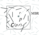
(a)

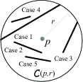
(b)

Figure 4: Example of pruing obstacles. (a) The rectangle denotes the MBR of ${C}(p,r)$, and the black solid line segments denote initial candidate obstacles. (b) The black solid line segments denote candidate obstacles.

We say the rest of obstacles (after pruning) are candidate obstacles. In particular, they can be generally classified into five types, see Figure 4(b). We remark that it is also feasible to develop more complicated pruning mechanism that can prune the Case 4-type obstacle.

In particular, we can easily realize an obvious characteristic — all these candidate obstacles are bounded by the circle ${C}(p,r)$. This fact lets us be without distraction from handling many unrelated obstacles, and be easier to construct the CVR. In the next subsection, we show how to construct it and store its boundaries in the aforementioned (well-known) data structure — double linked list.

III-B2 Constructing

The basic idea of constructing the CVR is based on the rotational plane sweep [37]. We first introduce some basic concepts, for ease of understanding the detailed process of constructing the CVR.

Given the circle $C(p,r)$, we use $L$ to denote a horizontal ray emitting from $p$ to the right of $p$. When we rotate $L$ around $p$, we call the obstacles that currently intersect with $L$ the active obstacles. Assume that $L$ intersects with an obstacle at $u$, we use $o(u)$ to denote this obstacle. Let $T$ be a balance tree, we shall insert the active obstacles into $T$. Assume that $o(e_{i})$ is a node in $T$, we use $o(e_{j})$ to denote the parent node of $o(e_{i})$ in $T$ by default. Given an obstacle endpoint $e$ and the horizontal ray $L$, we use $\angle(e)$ to denote the counter-clockwise angle subtended by the segment $\overline{pe}$ and the ray ${L}$. We say this angle is the polar angle of $e$. Given two endpoints $e$ and $e^{\prime}$ of an obstacle $o$, if $\angle(e)>\angle(e^{\prime})$, we say $e$ is the upper endpoint and $e\prime$ is the lower endpoint; and vice verse. Moreover, let $\mathscr{D}$ be a double linked list used to store the CVR.

We remark that two endpoints of an obstacle $o$ can have the same size of polar angles; this problem can be solved by directly ignoring $o$, since this obstacle $o$ almost makes no impact on the size of ${\mathscr{R}}_{cvr}(p,r)$. In the subsequent discussion, we assume two endpoints of any obstacle $o$ have different polar angles.

Theorem III.3.

Given a circle ${C}(p,r)$, without loss of generality, assume that there are $n^{\prime}(\leq n)$ candidate obstacles; then constructing ${\mathscr{R}}_{cvr}({p},{r})$ can be finished in $O(n\log n)$ time.

Proof.

We first draw the horizontal ray ${L}$ from $p$ to the right of $p$, and then compute the intersections between ${L}$ and all candidate obstacles, which takes $O(n^{\prime})$ time in the worst case. Without loss of generality, assume that there are $k$ intersections. Let $u_{i}$ denote one of these intersections, we sort these intersections such that $dist(p,u_{i-1})<dist(p,u_{i})<dist(p,u_{i+1})$ for any $i\in[2,3,$ $\cdots,k-1]$. (Note that, these active obstacles are also being sorted when we sort the intersections.) This takes $O(n^{\prime}\log n^{\prime})$ time, sine $k$ can have $\Omega(n^{\prime})$ size in the worst case, see Figure 5(a).

We then insert these active obstacles ${o}(u_{i})$ ($i\in[1,\cdots,k]$) into the balance tree $T$ such that, if $o(u_{i})$ is the left (right) child of $o(u_{j})$, then $i<j$ ($i>j$). So, $o(u_{1})$ is the leftmost leaf of $T$. (Note that, any point $p^{*}\in o(u_{i})$ is visible from $p$ if and only if $o(u_{i})$ is the leftmost leaf in $T$.) Initializing the tree $T$ takes $O(n^{\prime})$ time, since $|T|=k=\Omega(n^{\prime})$ in the worst case.

We sort the endpoints of all candidate obstacles according to their polar angles. We denote these sorted endpoints as $e_{1}$, $e_{2}$, $\cdots$, $e_{2n^{\prime}}$ such that $\angle(e_{i-1})<$ $\angle(e_{i})<$ $\angle(e_{i+1})$ for any $i\in[2,3,\cdots,2n^{\prime}-1]$, see Figure 5(b). Since each obstacle has two endpoints, sorting them takes $O(n^{\prime}\log n^{\prime})$ time. We then rotate ${L}$ according to the counter-clockwise. Note that, in the process of rotation, the active obstacles in $T$ change if and only if $L$ passes through the endpoints of obstacles. We handle each endpoint event as follows.

 

1    if $e_{i}$ is the lower endpoint of obstacle $o(e_{i})$ then

2        Insert the obstacle $o(e_{i})$ into $T$

3        if $o(e_{i})$ is the leftmost leaf in $T$ then

4            if $|T|>1$ then

5                Let $z$ be the intersection between $\overline{pe_{i}}$ and $o(e_{j})~{}$

                  Put the two points $z$ and $e_{i}$ into ${\mathscr{D}}$ in order

6            else if $|T|=1$ $\land$ $dist(p,e_{i})\neq r$ then

7                Let $z$ be the intersection between $\overline{pe_{i}}$ and ${C}(p,r)$

                  Put the two points $z$ and $e_{i}$ into ${\mathscr{D}}$ in order

8            else // $|T|=1$ $\land$ $dist(p,e_{i})=r$

9                Put the point $e_{i}$ into ${\mathscr{D}}$

10   if $e_{i}$ is the upper endpoint of $o(e_{i})$ then

11       if $o(e_{i})$ is the leftmost leaf in $T$

12           if $|T|>1$ then

13               Let $z$ be the intersection between $\overline{pe_{i}}$ and $o(e_{j})$

                   Put the two points $e_{i}$ and $z$ into ${\mathscr{D}}$ in order

14           else if $|T|=1$ $\land$ $dist(p,e_{i})\neq r$ then

15               Let $z$ be the intersection between $\overline{pe_{i}}$ and ${C}(p,r)$

                   Let $z^{*}$ be a point such that $dist(p,z^{*})=r$ and $\overline{pz^{*}}$ is

                   subtended by $\overline{pe_{i}}$ and $\overline{pe_{i+1}}$

                   Put the three points $e_{i}$, $z$ and $z^{*}$ into ${\mathscr{D}}$ in order

16           else // $|T|=1$ $\land$ $dist(p,e_{i})=r$

17               Let $z^{*}$ be a point such that $dist(p,z^{*})=r$ and $\overline{pz^{*}}$ is

                   subtended by $\overline{pe_{i}}$ and $\overline{pe_{i+1}}$

                   Put the two points $e_{i}$ and $z^{*}$ into ${\mathscr{D}}$ in order

18       Remove $o(e_{i})$ from $T$

 

It is easy to know that the height of $T$ is $\log n^{\prime}$. So, each operation (e.g., insert, delete and find the active obstacle) in $T$ takes $O(\log n^{\prime})$ time. In addition, other operation (e.g., obtain the intersections $z$, $z^{*}$, and put them into ${\mathscr{D}}$) takes constant time. Thus, handling all endpoint events takes $n^{\prime}\log n^{\prime}$ time. After all endpoints are handled, we finally get the CVR whose boundaries are represented as a series of vertexes and appendix points (stored in ${\mathscr{D}}$). See Figure 5(b) for example, we shall get a series of organized points $\{e_{2},z_{1},z_{1}^{*},$ $z_{2},e_{3},e_{5},$ $z_{3},e_{6},z_{2}^{*},$ $z_{4},e_{7},$ $z_{5},e_{8}\}$, where $z_{1}^{*}$ and $z_{2}^{*}$ are appendix points.

We note that $n^{\prime}$ can have $\Omega(n)$ size in the worst case. In summary, constructing the CVR takes $O(n\log n)$ time. ∎

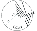
(a)

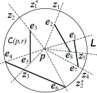
(b)

Figure 5: Example of constructing ${\mathscr{R}}_{cvr}(p,r)$. The black and grey solid line segment(s) denote candidate obstacles and the horizontal ray $L$, respectively. (a) $r$ denotes the radius of ${C}(p,r)$. (b) The dashed lines are the result of rotating $L$.

Discussion. Recall Section III-A, we mentioned two types of CVRs: ${\mathscr{R}}_{cvr}(s,l)$ and ${\mathscr{R}}_{cvr}(e,l-\pi(s,e))$. Regarding to the former, we use the circle ${C}(s,l)$ to prune unrelated obstacles and then to construct it based on the method discussed just now. Regarding to the latter, the circle ${C}(e,l-\pi(s,e))$ however, is unavailable beforehand. Hence, we first have to obtain this circle. In the next subsection, we show how to get it using a simple method.

III-B3 Obtaining the circle ${C}(e,l-\pi(s,e))$

This simple method incorporates the classical visibility graph technique. To save space, we simply state the previous results, and then use them to help us obtain this circle.

Definition III.1 (Visibility graph).

[38] The visibility graph of a set of $n$ line segments is an undirected graph whose vertexes consist of all the endpoints of the $n$ line segments, and whose edges connect mutually visible endpoints.

Lemma III.3.

[38] Given a set of $n$ line segments in $\mathbb{R}^{2}$, constructing the visibility graph for these segments can be finished in $O(n^{2})$ time.

Lemma III.4.

[7] Given an undirected graph with $n$ vertexes, finding the shortest path between any pair of vertexes can be finished in $O(n^{2})$ time using the standard Dijkstra algorithm.

To obtain the circle, our first step is to construct a visibility graph. Note that, we here need to consider the starting point $s$; in other words, the visibility graph consists of not only endpoints of obstacles but also the starting point $s$. Even so, from Lemma III.3, we can still get an immediate corollary below.

Corollary III.1.

Given a set $\mathscr{O}$ of $n$ disjoint line-segment obstacles, and the starting point $s$, we can build a visibility graph for the set of obstacles and the starting point $s$ in $O(n^{2})$ time.

Let $\mathscr{G}$ be the visibility graph obtained using the above method. For clarity, we say $C(e,l-\pi(s,e))$ is a valid circle if $l-\pi(s,e)>0$; otherwise, we say it is an invalid circle.

Theorem III.4.

Given the visibility graph $\mathscr{G}$, the maximum path length $l$, the staring point $s$, and an obstacle endpoint $e$, obtaining the circle ${C}(e,l-\pi(s,e))$ can be finished in $O(n^{2})$ time.

Proof.

It is easy to see that the key step of obtaining the circle $C(e,l-\pi(s,e))$ is to compute the shortest path length from $s$ to $e$, i.e., $\pi(s,e)$. Now assume we have obtained the visibility graph $\mathscr{G}$. At anytime we need to obtain the circle ${C}(e,l-\pi(s,e))$, we run the standard Dijkstra algorithm to find the shortest path from $s$ to $e$, which takes $O(n^{2})$ time, see Lemma III.4. Once the shortest path is found, its length $\pi(s,e)$ can be easily computed in additional $O(k)$ time, where $k$ is the number of segments in the path. Finally, if $l-\pi(s,e)>0$, we let $l-\pi(s,e)$ and $e$ be the radius and center of the circle, respectively, we get a valid circle; otherwise, we report it is an invalid circle. This can be finished in $O(1)$ time. Pulling all together, this completes the proof. ∎

III-C Putting it all together

The overall algorithm is shown in Algorithm 1. The correctness of our algorithm follows from Lemma III.2, Corollary III.1, Theorems III.1, III.3 and III.4.

Theorem III.5.

The running time of Algorithm 1 is $O(n^{3})$.

Proof.

Clearly, Lines 2, 3 and 4 take $O(n^{2})$, linear and $O(n\log n)$ time, respectively, see Corollary III.1, Theorems III.2 and III.3. Within the for circulation, Line 6 takes $O(n^{2})$ time, see Theorem III.4. Line 8 takes linear time, see Theorem III.2. Line 9 takes $O(n\log n)$ time, see Theorem III.3. We remark that the step “let $\mathscr{R}=\mathscr{R}\bigcup{\mathscr{R}}_{cvr}(e,l-\pi(s,e))$” shown in Line 8 is a simple boolean union operation of two polygons with circular arcs, it is used to remove the duplicate region. A straightforward adaptation of Bentley-Ottmann’s plane sweep algorithm [4], or the algorithm in [5] can be used to obtain their union in $O((m+k)\log m)$ time, where $m$ and $k$ respectively are the number of edges and intersections of the two polygons. Regarding to the case of our concern, $m=\Omega(n)$ and $k$ has the constant descriptive complexity, see e.g., Figure 5(b) for an illustration (note: substitute $C(p,r)$ with $C(s,l)$). Hence, the step “let $\mathscr{R}=\mathscr{R}\bigcup{\mathscr{R}}_{cvr}(e,l-\pi(s,e))$” actually can be done in $O(n\log n)$ time. Hence, the for circulation takes $O(n^{3})$ time. To summarize, the worst case upper bound of this algorithm is $O(n^{3})$. ∎

Algorithm 1 Finding Achievable Region of $\mathscr{M}$

0:  $\mathscr{O}$, $s$, $l$

0:  $\mathscr{R}$

1:  Set $\mathscr{R}=\emptyset$

2:  Construct the visibility graph $\mathscr{G}$

3:  Prune unrelated obstacles using ${C}(s,l)$

4:  Construct ${\mathscr{R}}_{cvr}(s,l)$, and let $\mathscr{R}={\mathscr{R}}_{cvr}(s,l)$

5:  for each obstacle endpoint $e$ do

6:     Obtain the circle ${C}(e,l-\pi(s,e))$

7:     if it is a valid circle then

8:        Prune unrelated obstacles using ${C}(e,l-\pi(s,e))$

9:        Construct ${\mathscr{R}}_{cvr}(e,l-\pi(s,e))$, and let $\mathscr{R}=\mathscr{R}\bigcup{\mathscr{R}}_{cvr}(e,l-\pi(s,e))$

10:  return  $\mathscr{R}$

Summary In this section, we have presented a simpler-version algorithm, which is indeed intuitive and easy-to-understand. We can easily see that the dominant step of this algorithm is to obtain the circle ${C}(e,l-\pi(s,e))$, i.e., Line 6. In the next section, we show how to break through this bottleneck and obtain an $O(n^{2}\log n)$ algorithm.

IV An $O(n^{2}\log n)$ Algorithm

This more efficient solution mechanically relies on the well-known technique called the shortest path map, which was previously used to compute the Euclidean shortest path among polygonal obstacles.

IV-A Overview of the short path map

Definition IV.1 (Shortest path map).

[23, 15] The shortest path map of a source point $s$ with respect to a set ${\mathscr{O}}$ of obstacles is a decomposition of the free space $\mathbb{R}^{2}\backslash$${\mathscr{O}}$ into regions, such that the shortest paths in the free space from $s$ to any two points in the same region pass through the same sequence of obstacle vertices.

The shortest path map is usually stored using the quad-edge data structure [13, 22, 15]. Let $SPM(s)$ denote the short path map of the source point $s$. It has the following properties.

Lemma IV.1.

[23, 24, 25] Once the $SPM(s)$ is obtained, the map can be used to answer the single-source Euclidean shortest path query in $O(\log n)$ time.

Lemma IV.2.

[23, 15] The map $SPM(s)$ has complexity $O(n)$, it consists of $O(n)$ vertexes, edges, and faces. Each edge is a segment of a line or a hyperbola.

The early method to compute $SPM(s)$ can be found in [22], the author (Mitchell) later adopted the continuous Dijkstra paradigm to compute this map [23, 25]. An optimal algorithm for computing the Euclidean shortest path among a set of polygonal obstacles was proposed by Hershberger and Suri [15], their method also used the continuous Dijkstra paradigm, but it employed two key ideas: a conforming subdivision of the plane and an approximate wavefront. Here we simply state the general steps of constructing $SPM(s)$, and their main result. (If any question, please refer to [15] for more details).

The general steps of constructing $SPM(s)$ can be summarized as follows.

It builds a confirming subdivision of the plane by considering only the vertexes of polygonal obstacles, dividing the plane into the linear-size cells.

It inserts the edges of obstacles into the subdivision above, and gets a confirming subdivision of the free space.

It propagates the approximate wavefront through the cells of the conforming subdivision of the free space, remembering the collisions arose from wavefront-wavefront events and wavefront-obstacle events.

It collects all the collision information, and uses them to determine all the hyperbola arcs of $SPM(s)$, and finally combines these arcs with the edges of obstacles, forming $SPM(s)$.

Lemma IV.3.

[15] Given a source point $s$, and a set $\mathscr{O}$ of polygonal obstacles with a total number $n$ of vertexes in the plane, the map $SPM(s)$ can be computed in $O(n\log n)$ time.

IV-B Constructing $SPM(s)$ among line-segment obstacles

The method to construct $SPM(s)$ among line-segment obstacles is the same as the one in [15].

To justify this, we can consider the line-segment obstacle as the special (or degenerate) case of the polygonal obstacle — one has only 2 sides and no area (see Figure 6 for an illustration). Furthermore, although the free space in the case of line-segment obstacles is (almost) equal to the space of the plane (since each obstacle here has no area), this fact still cannot against applying the algorithm in [15] to the case of our concern. This is mainly because (i) we can still build the confirming subdivision of the plane by considering only the endpoints of line segments firstly, and then insert the $n$ line segments into the conforming subdivision; (ii) the collisions are also arose from wavefront-wavefront events and wavefront-obstacle events, we can also collect these collision information, and then determine the hyperbola arcs of $SPM(s)$; and (iii) we can obtain $SPM(s)$ by (also) combining these arcs with the $n$ line segments. With the argument above, and each line-segment obstacle has only $2$ endpoints, from Lemma IV.3, we have an immediate corollary below.

Corollary IV.1.

Given a source point $s$, and a set $\mathscr{O}$ of $n$ line-segment obstacles in the plane, the map $SPM(s)$ can be computed in $O(n\log n)$ time.

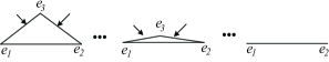
Figure 6: The line-segment obstacle is the degenerate case of the polygonal obstacle.

IV-C The algorithm

To obtain the achievable region $\mathscr{R}$, the first step of this $O(n^{2}\log n)$ algorithm is to construct $SPM(s)$. The rest of steps are the same as the ones in Algorithm 1 except the step “obtain the circle $C(e,l-\pi(s,e))$”. We now can obtain this circle in a more efficient way. This is mainly because the short path can be computed in $O(\log n)$ time once $SPM(s)$ is available, see Lemma IV.1. Based on this fact and the previous analysis used to prove Theorem III.4, we can easily build the following theorem.

Theorem IV.1.

Given the short path map $SPM(s)$, the maximum path length $l$, and an obstacle endpoint $e$, obtaining the circle ${C}(e,l-\pi(s,e))$ can be finished in $O(\log n)$ time.

The correct of this algorithm follows from Algorithm 1, Corollary IV.1 and Theorem IV.1. The pseudo codes are shown in Algorithm 2.

Algorithm 2 Finding Achievable Region of $\mathscr{M}$

0:  $\mathscr{O}$, $s$, $l$

0:  $\mathscr{R}$

1:  Set $\mathscr{R}=\emptyset$

2:  Construct $SPM(s)$

3:  Prune unrelated obstacles using ${C}(s,l)$

4:  Construct ${\mathscr{R}}_{cvr}(s,l)$, and let $\mathscr{R}={\mathscr{R}}_{cvr}(s,l)$

5:  for each obstacle endpoint $e$ do

6:     Obtain the circle ${C}(e,l-\pi(s,e))$ based on $SPM(s)$

7:     if it is a valid circle then

8:        Prune unrelated obstacles using ${C}(e,l-\pi(s,e))$

9:        Construct ${\mathscr{R}}_{cvr}(e,l-\pi(s,e))$, and let $\mathscr{R}=\mathscr{R}\bigcup{\mathscr{R}}_{cvr}(e,l-\pi(s,e))$

10:  return  $\mathscr{R}$

Theorem IV.2.

The running time of Algorithm 2 is $O(n^{2}\log n)$.

Proof.

This follows directly from Theorem IV.1 and the proof for Theorem III.5. ∎

Summary. This section presented an $O(n^{2}\log n)$ algorithm by modifying Algorithm 1. We can easily see that the dominant step has shifted, compared to Algorithm 1. Now, The bottleneck is located in Line 9, which takes $O(n\log n)$ time. In the next section, we show how to improve this $O(n^{2}\log n)$ algorithm to obtain a sub-quadratic algorithm.

V An $O(n\log n)$ Algorithm

The first step of this $O(n\log n)$ algorithm is also to construct the short path map, which is the same as the one in Algorithm 2. It however, does not construct the CVRs. Instead, it directly traverses each region of the short path map to obtain their boundaries, and finally merges them.

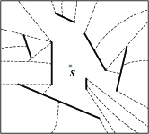
(a)

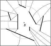
(b)

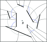
(c)

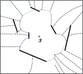
(d)

Figure 7: Illustration of $SPM(s)$. (a) The kernel-region. (b) The circular kernel-region $\mathscr{R}_{map}$ actually equals the circular visibility region $\mathscr{R}_{cvr}(s,l)$. (c) No duplicate region is needed to be handled. (d) The merged result.

V-A Regions of $SPM(s)$

As mentioned in Section IV-A, for two different points $p$ and $p^{\prime}$ in the same region, their short paths (i.e., $\pi(s,p)$ and $\pi(s,p^{\prime})$) pass through the same sequence of obstacle vertices. We say the final obstacle vertex (among the sequence of obstacle vertexes) is the control point of this region. Let $e_{c}$ be a control point, we say $e_{c}$ is a valid control point if $\pi(s,e_{c})<l$; otherwise, we say it is an invalid control point.

For ease of discussion, we say the region containing the starting (source) point $s$ is the kernel-region, and use $\mathscr{R}_{map}(k)$ to denote this region. We say any other region is the ordinary region, and use $\mathscr{R}_{map}(o)$ to denote an ordinary region of $SPM(s)$. Intuitively, the kernel-region can have $\Omega(n)$ edges in the worst case (see e.g., Figure 7(a)), and the number of edges of an ordinary region has the constant descriptive complexity.

Moreover, we say the intersection set of the kernel-region $\mathscr{R}_{map}(k)$ and the circle $C(s,l)$ is the circular kernel-region, and denote it as $\mathscr{R}_{map}^{*}(k)$. Assume that $c_{e}$ is a valid control point of an ordinary region $\mathscr{R}_{map}(o)$, we say the intersection set of this ordinary region and the circle $C(s,l-\pi(s,c_{e}))$ is the circular ordinary region, and denote it as $\mathscr{R}_{map}^{*}(o)$. According to the definition of $SPM(s)$, $R_{map}^{*}(k)$ and $R_{map}^{*}(o)$, we can easily build the following theorem.

Theorem V.1.

Given $SPM(s)$ and the maximum path length $l$, without loss of generality, assume that there are a set $\Psi$ of ordinary regions (among all the ordinary regions) such that each of these regions has the valid control point $e_{c}$ (i.e., $l-\pi(s,e_{c})>0$), implying that there are a number $|\Psi|$ of circular ordinary regions. Let $\Psi^{*}$ be the set of circular ordinary regions. Then, the achievable region $\mathscr{R}$ can be computed as $\mathscr{R}=\mathscr{R}_{map}^{*}(k)\bigcup_{\mathscr{R}_{map}*(o)\in\Psi^{*}}\mathscr{R}_{map}^{*}(o)$.

Lemma V.1.

Given the kernel-region $\mathscr{R}_{map}(k)$ and the circle $C(s,l)$, computing their intersection set can be done in $O(n)$ time.

Proof.

This stems directly from the fact that the kernel-region $\mathscr{R}_{map}(k)$ can have $\Omega(n)$ edges in the worst case, and computing their intersections takes linear time. ∎

Lemma V.2.

Given an ordinary region $\mathscr{R}_{map}(o)$ and its control point $e_{c}$, we assume that $e_{c}$ is a valid control point. Then, computing the intersection set of this ordinary region and the circle $C(c_{e},l-\pi(s,e_{c}))$ can be done in constant time.

Proof.

The proof is the similar as the one for Lemma V.1. ∎

Lemma V.3.

Given $SPM(s)$, finding the control point of any ordinary region can be finished in $O(\log n)$ time.

Proof.

We just need to randomly choose a point in the region and execute a Euclidean shortest path query, the final obstacle vertex in the path can be obtained easily. The Euclidean shortest path query can be done in $O(\log n)$ time, see Lemma IV.1. ∎

Discussion. Recall Section III-A, we mentioned two types of circular visibility regions. We remark that the circular kernel-region $\mathscr{R}_{map}^{*}(k)$ actually equals the circular visibility region $\mathscr{R}_{cvr}(s,l)$, see Figure 7(b). However, the circular ordinary region $\mathscr{R}_{map}^{*}(o)$ does not equal another type of circular visibility region $\mathscr{R}_{cvr}(e,l-\pi(s,e))$. More specifically, (i) $|\mathscr{E}^{\prime}|$ (see Theorem III.1) is usually less than $|\Psi^{*}|$ (see Theorem V.1); and (ii) the intersection set of two circular visibility regions may be non-empty (i.e., they may have the duplicate region), but the intersection set of any two circular ordinary regions (or, any circular ordinary region and circular kernel-region) is empty (see e.g., Figure 7(c)), implying that no duplicate region is needed to be removed, hence in theory, we can directly output all the circular ordinary regions and the circular kernel-region. The output shall be a set of conic polygons, since the boundaries of some circular ordinary regions possibly consist of not only circular arc and straight line segments but also hyperbolas. But we should note that Section II previously has stated a constraint — the output of the algorithm to be developed is the well-organized boundaries of the achievable region $\mathscr{R}$ (just like shown in Figure 7(d)), rather than a set of out-of-order segments, implying that we need to handle edges (or segments) of those conic polygons. Even so, we still can obtain an $O(n\log n)$ worst case upper bound, since the number of segments among all these conic polygons has only complexity $O(n)$.

V-B The algorithm

The final algorithm is shown in Algorithm 3. Its correctness directly follows from Corollary IV.1, Theorem IV.1, and Theorem V.1.

Algorithm 3 Finding Achievable Region of $\mathscr{M}$

0:  $\mathscr{O}$, $s$, $l$

0:  $\mathscr{R}$

1:  Set $\mathscr{R}=\emptyset$

2:  Construct $SPM(s)$

3:  Obtain $\mathscr{R}_{map}^{*}(k)$

4:  for each ordinary region $\mathscr{R}_{map}(o)$ do

5:     Obtain the control point of $\mathscr{R}_{map}(o)$

6:     if it is a valid control point  then

7:        Obtain $\mathscr{R}_{map}^{*}(o)$

8:  Let $\mathscr{R}=\mathscr{R}_{map}^{*}(k)\bigcup_{\mathscr{R}_{map}*(o)\in\Psi^{*}}\mathscr{R}_{map}^{*}(o)$ // i.e., merge all the regions obtained before

9:  return  $\mathscr{R}$

Theorem V.2.

The running time of Algorithm 3 is $O(n\log n)$.

Proof.

We can easily see that, Lines 2 and 3 take $O(n\log n)$ and linear time respectively, see Corollary IV.1 and Lemma V.1. In the for circulation, Lines 5 and 6 take $O(\log n)$ time, see Lemma V.3. We remark that Line 6 actually is (almost) the same as the operation — determining if $C(e,l-(s,e))$ is a valid circle, see Theorem IV.1. Moreover, Line 7 takes constant time, see Lemma V.2. Note that, the number of ordinary regions is the linear-size complexity, which stems directly from Lemme IV.2. So, the overall execution time of the for circulation is also $O(n\log n)$. Finally, Line 8 is a simple boolean set operation, which can be done in $O(n\log n)$ time, since the number of edges of all these conic polygons has complexity $O(n)$, arranging all these segments and appealing to the algorithm in [5] can immediately produce their union in $O((n+i)\log n)$ time, where $i$ is the number of intersections among all these segments. Note that in the context of our concern, $i$ has the linear complexity, see e.g., Figure 7(c) for an illustration. This completes the proof. ∎

Summary. This section presented our final algorithm, which significantly improves the previous ones. We remark that, maybe there still exist more efficient solutions to improve some sub-steps in Algorithm 3, but it is obvious that beating this worst case upper bound is (almost) impossible, this is mainly because, the nature of our problem decides any solution to be developed, or the ones proposed in this paper, (almost) cannot be free from computing the geodesic distance, i.e., the shortest path length in the presence of obstacles. Moreover, we remark that although our attention is focused on the case of disjoint line-segment obstacles in this paper, it is not difficult to see that all these algorithms can be easily applied to the case of disjoint polygonal obstacles (directly or after the minor modifications). Finally, the $O(n\log n)$ algorithm is to construct $SPM(s)$ with respect to all the obstacles, sometimes the maximum path length $l$ is possibly pretty small, an output-sensitive algorithm can be easily developed by a straightforward extension of this $O(n\log n)$ algorithm.

VI Concluding remarks

This paper proposed and studied the FAR problem. In particular, we focused our attention to the case of line-segment obstacles. We first presented a simpler-version algorithm for the sake of intuition, which runs in $O(n^{3})$ time. The basic idea of this algorithm is to reduce our problem to computing the union of a series of circular visibility regions (CVRs). We demonstrated its correctness, analysed its dominant steps, and improved it by appealing to the shortest path map (SPM) technique, which was previously used to compute the Euclidean shortest path among polygonal obstacles. We showed Hershberger-Suri’s method can be equivalently used to compute the SPM in the case of our concern, and thus immediately yielded an $O(n^{2}\log n)$ algorithm. Owing to the realization above, the third algorithm also used this technique. It however, did not construct the CVRs. Instead, it directly traversed each region of the SPM to trace the boundaries, thus obtained the $O(n\log n)$ worst case upper bound.

We conclude this paper with several open problems.

The dynamic version of this problem is that, if the maximum path length $l$ is not constant, how to efficiently maintain the dynamic achievable region?

The inverse problem is that, given a closed region ${\mathscr{R}}^{*}$, how to efficiently determine whether or not ${\mathscr{R}}^{*}$ is the real achievable region ${\mathscr{R}}$?

The multi-object version of this problem is that, if there are multiple moving objects, how to efficiently find their common part of their achievable regions?

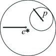
(a)

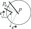
(b)

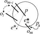
(c)

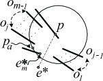
(d)

Figure 8: Illustration of Lemma III.1. (a) The small and big circles denote ${C}(p,l-\pi(s,p))$ and ${C}(e^{*},l-\pi(s,e^{*}))$, respectively. In (b-d), we omit the circle ${C}(e^{*},l-\pi(s,e^{*}))$ for clearness.

A. The proof of Lemma III.1

Proof.

There are several cases for a point $p$ $\in C(s,l)$ such that $\pi(s,p)<l$.

$\bullet$ Case 1: $\underline{p\in\mathscr{E}^{\prime}}$. In this case, it is obvious that ${\mathscr{R}}_{cvr}(p,l-\pi(s,p))\subset\bigcup_{e\in\mathscr{E}^{\prime}}{\mathscr{R}}_{cvr}(e,l-\pi(s,e))\bigcup{\mathscr{R}}_{cvr}(s,l)$.

$\bullet$ Case 2: $p$ is located in one of obstacles but $p\notin\mathscr{E}^{\prime}$ . Without loss of generality, assume that $e^{*}$ is the previous point on the shortest path from $s$ to $p$ such that $e^{*}\in\{s\bigcup\mathscr{E}^{\prime}\}$. Consider the two circles $C(p,l-\pi(s,p))$ and $C(e^{*},l-\pi(s,e^{*}))$. It is easy to know that $dist(p,e^{*})+(l-\pi(s,p))=l-\pi(s,e^{*})$ and $p\in C(e^{*},l-\pi(s,e^{*}))$. Hence, ${C}(p,l-\pi(s,p))$ must be an inscribed circle of ${C}(e^{*},l-\pi(s,e^{*}))$. This implies that ${C}(p,l-\pi(s,p))\subset{C}(e^{*},l-\pi(s,e^{*}))$. Therefore, we get a preliminary conclusion — for any point $p_{a}$ such that $p_{a}\in{\mathscr{R}}_{cvr}(p,l-\pi(s,p))$ and $\sphericalangle(p_{a},e^{*})$, we have that $p_{a}\in{\mathscr{R}}_{cvr}(e^{*},l-\pi(s,e^{*}))$.

$\star$ Case 2.1: There is no other obstacle that makes impact on the size of ${\mathscr{R}}_{cvr}(p,l-\pi(s,p))$. See Figure 8(a). Clearly, for any point $p_{a}\in\mathscr{R}_{cvr}(p,l-\pi(s,p))$, we have $\sphericalangle(p_{a},e^{*})$. By the preliminary conclusion shown in the previous paragraph, this completes the proof of Case 2.1.

$\star$ Case 2.2: There are other obstacles that make impact on the size of ${\mathscr{R}}_{cvr}(p,l-\pi(s,p))$. The key of point is to prove that, for any point $p_{a}$ such that $p_{a}\in{\mathscr{R}}_{cvr}(p,l-\pi(s,p))$ and $\lnot(\sphericalangle(p_{a},e^{*}))$, it must be located in a circular visibility region whose center is the endpoint of certain obstacle. Let $\mathscr{O}^{\prime}$ be the set of other obstacles that make impact on the size of ${\mathscr{R}}_{cvr}(p,l-\pi(s,p))$. For ease of discussion, assume that $e^{*}_{i}$ and $e^{\prime}_{i}$ are the endpoints of the $i$th obstacle (among $|\mathscr{O}^{\prime}|$ obstacles). Let $e^{*}_{i}$ denote the endpoint such that $\pi(e^{*},e^{*}_{i})\leq\pi(e^{*},e^{\prime}_{i})$. Let $m^{\prime}=|\mathscr{O}^{\prime}|$, and $m$ be an arbitrary integer. We next prove by induction that the following proposition called $\mathbb{P}$ holds — for any point $p_{a}$ such that $p_{a}\in{\mathscr{R}}_{cvr}(p,l-\pi(s,p))$ and $\lnot(\sphericalangle(p_{a},e^{*}))$, we have that $p_{a}\in\bigcup_{i=1}^{m^{\prime}}{\mathscr{R}}_{cvr}(e^{*}_{i},l-\pi(s,e^{*}_{i}))$.

We first consider $m^{\prime}=1$. We connect the following points, $e^{*}$, $p$, $p_{a}$ and $e^{*}_{1}$. Then, they build a circuit with four edges (see Figure 8(b)). Let $\Delta$ be ($dist(e^{*},p)$+$dist(p,p_{a})$)$-$($dist(e^{*},e^{*}_{1})$+ $dist(e^{*}_{1},p_{a})$). According to analytic geometry and graph theory, it is easy to know that $\Delta>0$. This implies that the radius of ${\mathscr{R}}_{cvr}(e^{*}_{1},l-\pi(s,e^{*}_{1}))$ is equal to $dist(e_{1}^{*},p_{a})+\Delta$. So, for any point $p_{a}$ such that $p_{a}\in{\mathscr{R}}_{cvr}(p,l-\pi(s,p))$ and $\lnot(\sphericalangle(p_{a},e^{*}))$, we have that $p_{a}\in{\mathscr{R}}_{cvr}(e^{*}_{1},l-\pi(s,e^{*}_{1}))$. Therefore, the proposition $\mathbb{P}$ holds when $m^{\prime}=1$.

By convention, we assume $\mathbb{P}$ holds when $m^{\prime}=m-1$. We next show it also holds when $m^{\prime}=m$. Let $o_{1}$, $\cdots$, $o_{m}$ denote these obstacles, i.e., $\mathscr{O}^{\prime}=\{o_{1},\cdots,o_{m}\}$. We remark that (i) it corresponds to “$m^{\prime}=m-1$” if $o_{m}$ viewed from $p$ is totally blocked by other $m-1$ obstacles; and (ii) in the rest of the proof, unless stated otherwise, we use “viewed from $p$” by default when the location relation of obstacles is considered. There are three cases.

First, if $o_{m}$ is disjointed with other $m-1$ obstacles, we denote by $\asymp(o_{m},\bigcup_{i=1}^{m-1}o_{i})$ this case. See Figure 8(c). Let’s consider $o_{m}$, according to the method for proving the case $m^{\prime}=1$, it is easy to get a result — for any point $p_{a}$ such that $p_{a}\in{\mathscr{R}}_{cvr}(p,l-\pi(s,p))$ and $p_{a}\notin\bigcup_{i=1}^{m-1}{\mathscr{R}}_{cvr}(e^{*}_{i},l-\pi(s,e^{*}_{i}))$ and $\lnot(\sphericalangle(p_{a},e^{*}))$, we have that $p_{a}\in{\mathscr{R}}_{cvr}(e^{*}_{m},l-\pi(s,e^{*}_{m}))$. Furthermore, we have assumed $\mathbb{P}$ holds when $m^{\prime}=m-1$. This completes the proof of the case $\asymp(o_{m},\bigcup_{i=1}^{m-1}o_{i})$.

Second, if $o_{m}$ is in the front of other $m-1$ obstacles, we denote by $\succ(o_{m},\bigcup_{i=1}^{m-1}o_{i})$ this case. We connect the points $e^{*}$, $\cdots$, $e_{i}^{*}$, $\cdots$, and $e_{m}^{*}$ such that the set of segments build the shortest path from $e^{*}$ to $e_{m}^{*}$. The total length of these segments is $\pi(e^{*},e_{m}^{*})$. Without loss of generality, assume that $p_{a}$ is to be a point such that $p_{a}\in{\mathscr{R}}_{cvr}(p,l-\pi(s,p)$ and $p_{a}\notin\bigcup_{i=1}^{m-1}{\mathscr{R}}_{cvr}(e^{*}_{i},l-\pi(s,e^{*}_{i}))$ and $\lnot(\sphericalangle(p_{a},e^{*}))$. We also connect the points $e^{*}_{m}$ and $p_{a}$. Naturally, we get the shortest path from $e^{*}$ to $p_{a}$, its total length is $\pi(e^{*},e_{m}^{*})+dist(e_{m}^{*},p_{a})$. This implies that there is no other path (from $e^{*}$ to $p_{a}$) whose length is less than $\pi(e^{*},e_{m}^{*})+dist(e_{m}^{*},p_{a})$. Let $\Delta$ be $(\pi(e^{*},p)+dist(p,p_{a}))-(\pi(e^{*},e_{m}^{*})+dist(e_{m}^{*},p_{a}))$, we have that $l-\pi(s,e_{m}^{*})=dist(e_{m}^{*},p_{a})+\Delta>dist(e_{m}^{*},p_{a})$, since $\Delta>0$. Therefore, $p_{a}\in{\mathscr{R}}_{cvr}(e^{*}_{m},l-\pi(s,e^{*}_{m}))$. Furthermore, we have assumed $\mathbb{P}$ holds when $m^{\prime}=m-1$. This completes the proof of the case $\succ(o_{m},\bigcup_{i=1}^{m-1}o_{i})$.

Third, if $o_{m}$ is partially blocked by other $m-1$ obstacles. We denote by $\prec(o_{m},\bigcup_{i=1}^{m-1}o_{i})$ this case. Without loss of generality, assume that $o_{m}$ is partially blocked by an obstacle $o_{j}$. (i) If $o_{j}$ does not block any other $m-2$ obstacles (see, e.g., Figure 8(d)), according to the method for proving the case $m^{\prime}=1$, we can also get a result which is the same as the result shown in the case $\asymp(o_{m},\bigcup_{i=1}^{m-1}o_{i})$. (ii) Otherwise, we connect the points $e^{*}$, $\cdots$, $e_{i}^{*}$ ($i\in[1,\cdots,j-1]$), $\cdots$, and $e_{m}^{*}$ such that the set of segments build the shortest path from $e^{*}$ to $e_{m}^{*}$. The rest of steps are the same as the ones for proving the case $\succ(o_{m},\bigcup_{i=1}^{m-1}o_{i})$. And we can also get a result which is the same as the previous one. Furthermore, we have assumed the proposition $\mathbb{P}$ holds when $m^{\prime}=m-1$. This completes the proof of the case $\prec(o_{m},\bigcup_{i=1}^{m-1}o_{i})$.

In summary, the proposition $\mathbb{P}$ also holds when $m^{\prime}=m$. Combining the preliminary conclusion shown in the first paragraph of Case 2, this completes the proof of Case 2.2.

$\bullet$ Case 3: $p$ is not located in any obstacle. The proof for this case is almost the same as the one for Case 2. (Substituting the words “other obstacles” in Case 2 with “obstacles”.) Pulling all together, hence the lemma holds. ∎

References

- [1] C. C. Aggarwal and P. S. Yu. A survey of uncertain data algorithms and applications. IEEE Transactions on Knowledge and Data Engineering (TKDE), 21(5):609–623, 2009.
- [2] T. Asano. An efficient algorithm for finding the visibility polygon for a polygonal region with holes. Transactions of IECE of Japan E, 68(9):557–559, 1985.
- [3] T. Asano, T. Asano, L. J. Guibas, J. Hershberger, and H. Imai. Visibility-polygon search and euclidean shortest paths. In IEEE Symposium on Foundations of Computer Science (FOCS), pages 155–164, 1985.
- [4] J. L. Bentley and T. Ottmann. Algorithms for reporting and counting geometric intersections. IEEE Transaction on Computers (TC), 28(9):643–647, 1979.
- [5] E. Berberich, A. Eigenwillig, M. Hemmer, S. Hert, K. Mehlhorn, and E. Schömer. A computational basis for conic arcs and boolean operations on conic polygons. In European Symposium on Algorithm (ESA), pages 174–186. 2002.
- [6] R. Cheng, D. V. Kalashnikov, and S. Prabhakar. Querying imprecise data in moving object environments. IEEE Transactions on Knowledge and Data Engineering (TKDE), 16(9):1112–1127, 2004.
- [7] T. H. Cormen, C. E. Leiserson, R. L. Rivest, and C. Stein. Introduction To Algorithms, Second Edition. The MIT Press, Cambridge, 2001.
- [8] M. de Berg, O. Cheong, M. van Kreveld, and M. Overmars. Computational geometry: algorithms and applications, Third Edition. Springer, Berlin, 2008.
- [9] J. F. Eastman. An efficient scan conversion and hidden surface removal algorithm. Computers and Graphics (CG), 1(2-3):215–220, 1975.
- [10] M. L. Fredman and R. E. Tarjan. Fibonacci heaps and their uses in improved network optimization algorithms. Journal of the ACM (JACM), 34(3):596–615, 1987.
- [11] S. K. Ghosh. Visibility algorithms in the plane. Cambridge University Press, New York, 2007.
- [12] S. K. Ghosh and D. M. Mount. An output-sensitive algorithm for computing visibility graphs. SIAM Journal on Computing (SIAMCOMP), 20(5):888–910, 1991.
- [13] L. J. Guibas and J. Stolfi. Primitives for the manipulation of general subdivisions and computation of voronoi diagrams. ACM Transactions on Graphics (TOG), 4(2):74–123, 1985.
- [14] P. J. Heffernan and J. S. B. Mitchell. An optimal algorithm for computing visibility in the plane. SIAM Journal on Computing (SIAMCOMP), 24(1):184–201, 1995.
- [15] J. Hershberger and S. Suri. An optimal algorithm for euclidean shortest paths in the plane. SIAM Journal on Computing (SIAMCOMP), 28(6):2215–2256, 1999.
- [16] Y. K. Hwang and N. Ahuja. Gross motion planning - a survey. ACM Computing Surveys (CSUR), 24(3):219–291, 1992.
- [17] S. Kapoor and S. N. Maheshwari. Efficient algorithms for euclidean shortest path and visibility problems with polygonal obstacles. In ACM Symposium on Computational Geometry (SoCG), pages 172–182, 1988.
- [18] S. Kapoor, S. N. Maheshwari, and J. S. B. Mitchell. An efficient algorithm for euclidean shortest paths among polygonal obstacles in the plane. Discrete and Computational Geometry (DCG), 18(4):377–383, 1997.
- [19] A. Kolling, A. Kleiner, M. Lewis, and K. P. Sycara. Computing and executing strategies for moving target search. In IEEE International Conference on Robotics and Automation (ICRA), pages 4246–4253, 2011.
- [20] D. T. Lee and A. K. Lin. Computational complexity of art gallery problems. IEEE Transactions on Information Theory (TIT), 32(2):276–282, 1986.
- [21] D. T. Lee and F. P. Preparata. Euclidean shortest paths in the presence of rectilinear barriers. Networks, 14(3):393–410, 1984.
- [22] J. S. B. Mitchell. A new algorithm for shortest paths among obstacles in the plane. Annals of Mathematics and Artificial Intelligence (AMAI), 3(1):83–105, 1991.
- [23] J. S. B. Mitchell. Shortest paths among obstacles in the plane. In ACM Symposium on Computational Geometry (SoCG), pages 308–317, 1993.
- [24] J. S. B. Mitchell and C. H. Papadimitriou. The weighted region problem: Finding shortest paths through a weighted planar subdivision. Journal of the ACM (JACM), 38(1):18–73, 1991.
- [25] J. S. B. Mitchell and C. H. Papadimitriou. Shortest paths among obstacles in the plane. International Journal of Computational Geometry and Applications (IJCGA), 6(3):309–332, 1996.
- [26] J. O’Rourke. Art gallery theorems and algorithms. Oxford University Press, Oxford, 1987.
- [27] W. pang Chin and S. C. Ntafos. Optimum watchman routes. In ACM SIGACT/SIGGRAPH Symposium on Computational Geometry (SoCG), pages 24–33, 1986.
- [28] J. Pei, M. Hua, Y. Tao, and X. Lin. Query answering techniques on uncertain and probabilistic data: tutorial summary. In ACM International Conference on Management of Data (SIGMOD), pages 1357–1364, 2008.
- [29] E. Pitoura and G. Samaras. Locating objects in mobile computing. IEEE Transactions on Knowledge and Data Engineering (TKDE), 13(4):571–592, July/August 2001.
- [30] A. Ricci. An algorithm for the removal of hidden lines in 3d scenes. The Computer Journal (CJ), 14(4):375–377, 1971.
- [31] H. Rohnert. Shortest paths in the plane with convex polygonal obstacles. Information Processing Letters (IPL), 23(2):71–76, 1986.
- [32] J. Schiller and A. Voisard. Location-Based Services. Morgan Kaufmann Publishers, San Francisco, 2004.
- [33] M. Sharir and A. Schorr. On shortest paths in polyhedral spaces. In ACM Symposium on Theory of Computing (STOC), pages 144–153, 1984.
- [34] A. P. Sistla, O. Wolfson, S. Chamberlain, and S. Dao. Modeling and querying moving objects. In IEEE International Conference on Data Engineering (ICDE), pages 422–432. 1997.
- [35] J. A. Storer and J. H. Reif. Shortest paths in the plane with polygonal obstacles. Journal of ACM (JACM), 41(5):982–1012, 1994.
- [36] X. Sun, W. Yeoh, and S. Koenig. Efficient incremental search for moving target search. In International Joint Conference on Artificial Intelligence(IJCAI), pages 615–620, 2009.
- [37] S. Suri and J. O’Rourke. Worst-case optimal algorithms for constructing visibility polygons with holes. In ACM Symposium on Computational Geometry (SoCG), pages 14–23, 1986.
- [38] E. Welzl. Constructing the visibility graph for n-line segments in o(n2) time. Information Processing Letters (IPL), 20(4):167–171, 1985.