Current resonances in graphene with time dependent potential barriers

Abstract

A method is derived to solve the massless Dirac-Weyl equation describing electron transport in a mono-layer of graphene with a scalar potential barrier $U(x,t)$, homogeneous in the $y$-direction, of arbitrary $x$- and time dependence. Resonant enhancement of both electron backscattering and currents, across and along the barrier, is predicted when the modulation frequencies satisfy certain resonance conditions. These conditions resemble those for Shapiro-steps of driven Josephson junctions. Surprisingly, we find a non-zero $y$-component of the current for carriers of zero momentum along the $y$-axis.

Growing interest to graphene, see e.g. Ref. [reviews, ], is stimulated by many unusual and sometimes counter intuitive properties of this two dimensional material. Indeed, graphene supplies charge carriers exhibiting pseudo-relativistic dynamics of massless Dirac fermions. As one consequence the Klein tunneling phenomenon paradox occurs with unit probability through arbitrarily high and thick barriers at perpendicular incidence, irrespective of the particle energy, in accordance with experiment paradox-exp . The question arose how to control the electron motion in graphene and hence boosted detailed studies of Dirac fermions under the influence of various forms of scalar superl ; super5 ; left ; peeters09b ; pnexperiments or vector magstruc potentials.

Applying a time-dependent laser field to pristine graphene opens an alternative and efficient way Efetov ; laser1 ; laser2 to control spectrum and transport properties. It was shown Efetov that Dirac fermions accross $p$-$n$-junctions can aquire an effective mass when driven by a laser field. This results in an exponential suppression of chiral tunneling even for perpendicular incidence upon the junction, if the ac-electric field is directed parallel to the junction, in stark contrast to Klein tunneling occuring in the absence of the laser field. Actually, time dependent laser fields can mimic laser2 the influence of any electrostatic graphene superlattices on the electron spectrum in graphene. The question arises whether and under which conditions time-dependent modulations of an electrostatic barrier, where energy is not conserved, would affect electron transport and generate backscattering.

In this Letter we answer this question by solving the problem for arbitrary space-time dependent scalar potentials $U(x,t)$. Our solution is based on expanding the wave function as a power series with respect to the momentum $k_{y}$ parallel to the barrier, and manifests a structure of left and right moving waves. All terms appearing in the $k_{y}$-expansion can be calculated analytically, despite of the fact that each term is described by a partial differential equation in $(x,t)$-space. At $k_{y}=0$ (normal incidence upon the barrier) we confirm complete Klein tunneling for any $U(x,t)$ while for finite $k_{y}$ backscattering resonances can occur at certain angles of incidence, depending on the modulation frequency of the barrier. As a counter intuitive result we find a non-zero and oscillating current $j_{y}$ along the barrier, even at $k_{y}=0$ for valley polarized fermions. At $k_{y}\neq 0$ the current $j_{y}$ arises also in valley unpolarized situations, it can be resonantly amplified and flow in either direction. Interestingly, $j_{y}$ exhibits a non-zero dc-component at certain resonance frequencies, in full analogy to Shapiro-steps of driven Josephson junctions.

At low energies, the honeycomb lattice of graphene engenders two copies, $\tau_{z}=\pm 1$, of Dirac-Weyl Hamiltonians kanemele

$$H_{0}=v_{\mbox{\tiny F}}\>[\hat{\tau}_{z}\hat{\sigma}_{x}\hat{p}_{x}+\hat{\sigma}_{y}\hat{p}_{y}]\;,$$ (1)

centered about two inequivalent Dirac points (“valleys”) $K$ and $K^{\prime}$ at corners of the hexagonal first Brillouin zone where electron-hole symmetric bands touch; Pauli matrices $\hat{\sigma}_{x,y,z}$ act on two-component spinors representing sublattice amplitudes. Carriers near either of the Dirac points exhibit opposite Fermion helicities, $\>\bm{\sigma}\cdot\bm{p}/p=\pm 1\>$. Proposals exist in literature how to valley polarize carriers in graphene, by means of nanoribbons terminated by zig-zag edges zigzagribbons , by exploiting trigonal warping at elevated energies garcia08 , or by absorbing magnetic textures ziegler10 .

Smooth electromagnetic or disorder potentials ando98 , containing negligible fourier components at large wave vectors of the order of $|{\vec{K}}|$, will not cause scattering between valleys so that calculations can be carried out for $\tau_{z}=+1$ or $\tau_{z}=-1$ separately. Accordingly, time dependent potentials $U(x,t)$ should be slowly varying, without frequency components that might induce excursions to energies where the band structure of graphene starts deviating from the isotropic cone spectrum, i.e. below 0.6 eV zhou06 . Including $U(x,t)$, the Dirac equation for the wave function $\Psi_{k_{y}}(x,y,t)=\Psi(x,t)\exp(ik_{y}y)$ can be written in the form

$$\left(\begin{array}[]{cc}U(x,t)&-i\tau_{z}\frac{\partial}{\partial x}\\ -i\tau_{z}\frac{\partial}{\partial x}&U(x,t)\end{array}\right)\Psi+ik_{y}\left(\begin{array}[]{cc}0&-1\\ 1&0\end{array}\right)\Psi=i\frac{\partial}{\partial t}\Psi$$ (2)

where from now on we assume $v_{\mbox{\tiny F}}=1$ and $\hbar=1$. This equation has been solved analytically for time-independent potentials either by matching paradox of wave functions for rectangular barriers, or by the WKB method wkb-method for smooth barriers. Time dependent harmonic oscillations have been considered of gate voltages on either side of a graphene rectangle harmonicgates , of an electric field parallel to the barrier Efetov or in resonance approximation laser2 , or for some class of time dependent barriers $U(x,t)$ at $k_{y}=0$ solomon .

Our goal here is to construct the solution of eq. (2) for arbitrary $U(x,t)$ acting at positive times, $\>U(x,t<0)=0\>$. From the Ansatz

$$\Psi=\sum_{n=0}^{\infty}(ik_{y})^{n}\left(\begin{array}[]{c}1\\ \tau_{z}\end{array}\right)\Psi_{n,+}+\sum_{n=0}^{\infty}(ik_{y})^{n}\left(\begin{array}[]{c}1\\ -\tau_{z}\end{array}\right)\Psi_{n,-}$$ (3)

as a power series in $k_{y}$ we derive a recurrence relation for the coefficients $\Psi_{n,\pm}$ which obey the inhomogeneous first order partial differential equations,

$$\left(U(x,t)\mp i\frac{\partial}{\partial x}-i\frac{\partial}{\partial t}\right)\Psi_{n,\pm}\pm\tau_{z}\Psi_{n-1,\mp}=0\;,$$ (4)

with $\Psi_{-1,\pm}(x,t\geq 0)\equiv 0$. Initial conditions can be chosen as $\Psi_{0,\pm}(x,t=0)=a_{\pm}(x)=[\Psi_{A}(x,t=0)\pm\tau_{z}\Psi_{B}(x,t=0)]/2$, $\Psi_{n>0,\pm}=0$, where $\Psi_{A},\Psi_{B}$ describe electron amplitudes on either of the graphene sublattices. The two functions $a_{\pm}(x)$, providing the initial conditions, can be, e.g., a plane wave or a wave packet. We underline here the general structure of (3) as a sum of right $\Psi_{+}$ and left $\Psi_{-}$ moving waves. Using the standard d’Alembert’s ratio test, a sufficient criterion for convergence of series (3) is $|k_{y}|\lim_{n\rightarrow\infty}|\Psi_{n+1,\pm}|/|\Psi_{n,\mp}|<1$ for all relevant $x$ and $t$.

Despite of the fact that (4) are partial differential equations, we can solve them exactly using the method of characteristics couranthilbert . The corresponding result reads

$$\Psi_{n,\pm}(x,t)=a_{n,\pm}(x,t)e^{-i\int_{0}^{t}dt^{\prime}\;U(x\mp t\pm t^{\prime},t^{\prime})}$$ (5)

with $a_{0,\pm}=a_{\pm}(x\mp t)$ and

$$a_{n>0,\pm} = \mp i\tau_{z}\int_{0}^{t}dt^{\prime}\;\Psi_{n-1,\mp}(x\mp t\pm t^{\prime},t^{\prime})$$

$$\times e^{i\int_{0}^{t^{\prime}}dt^{\prime\prime}\;U(x\mp t\pm t^{\prime\prime},t^{\prime\prime})}\;.$$

Together with (3) the recursive solution for $\Psi_{n,\pm}$ provides the exact wave function $\Psi$ to any desired accurancy. To zeroth order approximation w.r.t. $k_{y}$ we obtain:

$$\psi(x,t)=a_{+}(x-t)\left(1\atop\tau_{z}\right)e^{-i\int_{0}^{t}dt^{\prime}\;U(x-t+t^{\prime},t^{\prime})}$$

$$\;\mbox{}+a_{-}(x+t)\left(1\atop-\tau_{z}\right)e^{-i\int_{0}^{t}dt^{\prime}\;U(x+t-t^{\prime},t^{\prime})}\;.$$ (6)

The first order corrections w.r.t. $k_{y}$ in (5) can be written as

$$a_{1,\pm}=\mp i\tau_{z}A_{1,\pm}=\mp i\tau_{z}\int_{0}^{t}dt^{\prime}\;a_{\mp}(x\mp t\pm 2t^{\prime})$$

$$\times e^{i\int_{0}^{t^{\prime}}dt^{\prime\prime}\;[U(x\mp t\pm t^{\prime\prime},t^{\prime\prime})-U(x\mp t\pm 2t^{\prime}\mp t^{\prime\prime},t^{\prime\prime})]}\;,$$ (7)

so that $\Psi=\Psi_{+}\left({1\atop\tau_{z}}\right)+\Psi_{-}\left({1\atop-\tau_{z}}\right)$ as in (3), with

$$\Psi_{\pm}=[a_{0,\pm}\pm k_{y}\tau_{z}A_{1\pm}]e^{-i\int_{0}^{t}dt^{\prime}\>U(x\mp t\pm t^{\prime},t^{\prime})}\;.$$ (8)

When $k_{y}=0$ and when the wave packet is initially purely right moving, $\>a_{-}=0\>$, eq. (6) reveals that the electron density distribution $\>|a_{+}(x-t)|^{2}\>$ undistortedly continues to propagate to the right without reflection: $\Psi_{-}(x,t)=0$ for all times $t>0$. This proves complete Klein tunneling also in the presence of time dependent barriers; wave functions $\Psi_{\pm}$ acquire only a phase factor by the potential at $k_{y}=0$.

As a measurable quantity, we now evaluate the current density in cartesian components, $j_{x}=\Psi^{*}\tau_{z}\sigma_{x}\Psi=2\Psi_{+}^{*}\Psi_{+}-2\Psi_{-}^{*}\Psi_{-}=j_{0x}+j_{1x}$ and $j_{y}=\Psi^{*}\sigma_{y}\Psi=2i\tau_{z}(\Psi_{+}^{*}\Psi_{-}-\Psi_{+}\Psi_{-}^{*})=j_{0y}+j_{1y}$. Here, the last equal signs refer to zeroth and first order contributions w.r.t. $k_{y}$, respectively, yielding

$$j_{0x}=2(|a_{0+}|^{2}-|a_{0-}|^{2})$$ (9)

$$j_{0y}=4\tau_{z}|a_{0+}a_{0-}|\sin(\varphi+\phi_{0})$$ (10)

$$j_{1x}=4k_{y}\tau_{z}\Re{\rm e}\{a_{0+}A_{1+}^{*}-a_{0-}A_{1-}^{*}\}$$ (11)

$$j_{1y}=4k_{y}\left(|A_{1+}a_{0-}^{*}|\sin(\varphi-\phi_{-})-|A_{1-}^{*}a_{0+}|\sin(\varphi+\phi_{+})\right)$$ (12)

with $\varphi=\int_{0}^{t}[U(x+t-t^{\prime},t^{\prime})-U(x-t+t^{\prime},t^{\prime})]dt^{\prime}$, $\phi_{0}={\rm arg}(a_{0+}a_{0-}^{*})$, and $\phi_{\pm}={\rm arg}(a_{0\pm}A_{1\mp}^{*})$. We distinguish two cases: (i) $\tau_{z}$-independent contributions $j_{0x}$ and $j_{1y}$ which can be observed for valley unpolarized carriers and (ii) $\tau_{z}$-dependent contributions $j_{1x}$ and $j_{0y}$ where detection calls for valley polarization.

Eqs. (9) and (10) describe the current density at normal incidence, $k_{y}=0$. Then $j_{x}$ stays unaffected by the barrier, irrespective of $\tau_{z}$ which rephrases the above result of complete Klein tunneling. Surprisingly, a current $j_{y}$ flows perpendicular to the momentum in graphene, provided the sample is valley polarized (the total current $\bm{j}=\bm{j}^{+}+\bm{j}^{-}$, where $\bm{j}^{\tau_{z}}$ originates from states near valley $K$ ($\tau_{z}=+1$) or $K^{\prime}$ ($\tau_{z}=-1$), respectively). This current (10) results from interfering left and right moving waves, which both need to have nonzero amplitudes, $a_{0+}a_{0-}\neq 0$.

Eqs. (11) and (12) describe corrections to the current density at small but finite angles of incidence, $k_{y}\neq 0$. Thereby, $j_{1x}$ exhibits qualitatively similar properties as $j_{0y}$; in particular it stays nonvanishing at finite valley polarization only. By contrast, the current density $j_{1y}$ now exhibits striking current oscillations and current reversals already in valley unpolarized situations as we show in more detail below.

Next we turn to the question how carriers are reflected by $U(x,t)$. Let’s consider an initially right moving plane wave, $\Psi_{k_{y}}=e^{i(k_{x}x+k_{y}y)}\left({1\atop\tau_{z}}\right)$ at $t=0$ which produces a current density $j_{0x}=+2$ pointing to the right. Using equations (3) and (8), and assuming small $k_{y}$, the leading contribution to the reflected current density $j_{2x}=-k_{y}^{2}|A_{1-}|^{2}$ arises in ${\cal O}(k_{y}^{2})$ under the action of the barrier at $t>0$ and is proportional to $|j_{0x}|$, cf. (7,9). This suggests to employ the ratio

$$R(x,t):=-j_{2x}/j_{0x}=k_{y}^{2}|A_{1-}(x,t)|^{2}/2$$ (13)

as a measure for the reflectivity at small $k_{y}$. While the quantity $R(x,t)$ evolves in time, together with $U(x,t)$, it is independend of $\tau_{z}$ and, thus, measurable without valley polarization. Moreover, we also analyze the time averaged reflectivity $\>\overline{R}(x):=\>\lim_{T\rightarrow\infty}\int_{0}^{T}R(x,t)dt/T$, which can be measured just by means of dc-equipment.

In the following, two specific examples $U(x,t)=U^{(1,2)}(x,t)$ are considered. As initial conditions we take into account two cases: (i) a superposition of equal amplitudes of right and left propagating plane waves, $a_{\pm}=\exp(\pm ik_{x}x)$ and $\tau_{z}=+1$ when calculating $j_{0y}$; (ii) an incidently right moving wave $a_{+}=\exp(ik_{x}x),a_{-}=0$ when calculating $R$ and $j_{1y}$ for valley unpolarized systems. Our first example is $\>U^{(1)}(x,t)=U_{0}x\sin\omega t\>$. In view of (10), we derive for this case

$$\textstyle j_{0y}(x,t)=\>\sin 2\left[k_{x}x+U_{0}\left(\frac{t}{\omega}-\frac{\sin\omega t}{\omega^{2}}\right)\right]\;,$$ (14)

which can be rewritten as a sum

$$j_{0y}(x,t)=\sum_{n=-\infty}^{\infty}J_{n}\left(\frac{2U_{0}}{\omega^{2}}\right)\sin\left(2k_{x}x+\frac{2U_{0}t}{\omega}-n\omega t\right)\;,$$ (15)

using Bessel functions $J_{n}$. This form (15) reveals a peculiarity at $\omega=\omega_{n}$ with

$$\omega_{n}=\sqrt{2U_{0}/n}\;,\quad n\in\mathbb{N},$$ (16)

similar to Shapiro-steps tinkham of a driven Josephson junction. As depicted in Fig. 1a, frequencies $\omega=\omega_{n}$ generate periodic oscillations, which, again as in the case of Shapiro-steps, induce a nonzero dc-component in the current at given $x$. Modulating the potential with $\omega\neq\omega_{n}$ results in aperiodic oscillations and zero dc-component.

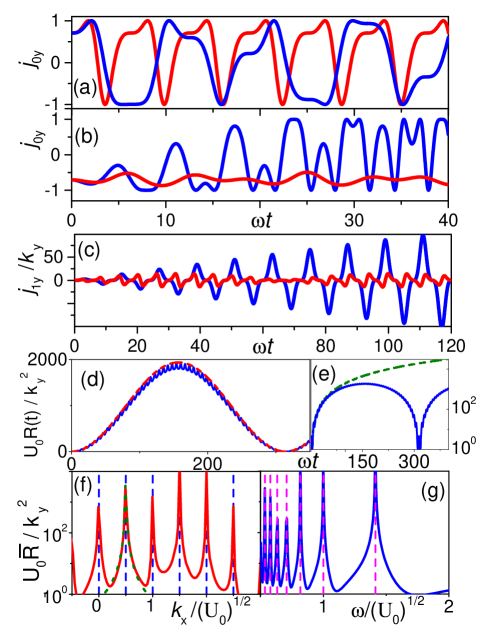
Figure 1: (Color online) (a) Current $j_{0y}$ (10) perpendicular to $\bm{k}$ versus time for $U^{(1)}(x,t)=U_{0}x\sin\omega t$, $k_{x}x=\pi/8$, and $U_{0}/\omega^{2}=1/\pi$ (blue line) and $U_{0}/\omega^{2}=1/2$ (red line), assuming a valley-polarized situation $\tau_{z}=1$. For “Shapiro-step” conditions (eq. (16)) periodic oscillations can be seen (red), while, away from this condition, aperiodic oscillations occur (blue). (b) Same as (a) but for potential $U^{(2)}(x,t)=U_{0}\cos(x/L)\cos\omega t$ with $x=\pi L/2,\ k=0,\ U_{0}L=0.1$, and frequencies $\omega=(\pi/2)(1/L)$ (red line) and $\omega=1/L$ (blue line). Both currents are aperiodic. For the matching condition $\omega=1/L$ (blue) a considerable enhancement followed by a saturation of the amplitude of the current oscillations occurs, while away from this resonance no enhancement is seen versus time. (c) Current $j_{1y}$ (12) for $U^{(1)}(x,t)$ at $x=0$, using $k=0$. At Shapiro-resonance ($U_{0}/\omega^{2}=1/2$, blue line) pronounced current enhancement occurs, cf. eqs. (Current resonances in graphene with time dependent potential barriers,18) while away from the resonance ($U_{0}/\omega^{2}=3/\pi$, red line) no enhancement is seen. (d) Time-dependent reflectivity $R(t)$, calculated by numerical integration of eq. (Current resonances in graphene with time dependent potential barriers), blue line, and by using the approximation (19), red dashed line, near resonance for $k_{x}/\sqrt{U_{0}}=0$ and $\omega^{2}/U_{0}=0.49$. (e) $R(t)$ at resonance (green dashed line, $k_{x}/\sqrt{U_{0}}=0,\omega^{2}/U_{0}=1/2$) and near resonance (blue line, $k_{x}/\sqrt{U_{0}}=0,\omega^{2}/U_{0}=0.49$). At the resonance, $R(t)$ increases with time $\sim t^{2}$, in agreement with equation (19). (f) Time-averaged reflectivity $\overline{R}$ as a function of $k_{x}/\sqrt{U_{0}}$ for $\omega/\sqrt{U_{0}}=1$. Equidistant resonances occur at $k_{x}/\sqrt{U_{0}}=1-n/2$ (dashed blue vertical lines), cf. eq. (18). One of the resonance peaks is well fitted by the resonance equation (20), as shown in dashed green. (g) $\overline{R}$ as a function of the driving frequency $\omega/\sqrt{U_{0}}$ for $k_{x}/\sqrt{U_{0}}=0$: resonance peaks are clearly seen at Shapiro-step conditions (18) $\omega/\sqrt{U_{0}}=\sqrt{2/n}$, indicated as dashed magenta vertical lines.

Similar resonance effects can also be seen in both, the reflectivity $R$ (13) and the current $j_{1y}$ (12). By inserting $U^{(1)}(x,t)$ into eq. (7) we derive

$$A_{1-} = e^{ik_{x}(x+t)}\int_{0}^{t}dt^{\prime}\>e^{-2ik_{x}t^{\prime}}e^{2iU_{0}(\omega t^{\prime}-\sin(\omega t^{\prime}))/\omega^{2}}$$

$$= e^{ik_{x}(x+t)}\sum_{n=-\infty}^{\infty}J_{n}\left(\frac{2U_{0}}{\omega^{2}}\right)\frac{e^{i(2U_{0}/\omega-2k_{x}-n\omega)t}-1}{i(2U_{0}/\omega-2k_{x}-n\omega)}\;,$$

from which we read off a Shapiro-step resonance condition

$$k_{n}=k_{x}=-\frac{n}{2}\omega+\frac{U_{0}}{\omega}\;,\quad n\in\mathbb{N}$$ (18)

specifying now a directional dependence of the momentum $\bm{k}$. From (Current resonances in graphene with time dependent potential barriers) together with (12) we conclude that in valley-unpolarized samples the current $j_{y}\propto k_{y}$ parallel to the barrier oscillates as a function of time and may take either sign (despite of the fixed $k_{y}$, see Fig. 1c). In addition, the amplitude of these oscillations increases with time as the Shapiro-step resonance condition (18) is met (compare red and blue curves in Fig. 1c).

Analogous resonances also show up in both reflectivities, $R$ and $\overline{R}$. The latter allows experimental observation of the here predicted behavior without time-domain measurements. Indeed, near the Shapiro-step resonance (18) we can keep only one summand in the expansion (Current resonances in graphene with time dependent potential barriers), yielding

$$R(t)=\frac{1}{2}k_{y}^{2}J_{n}^{2}\left(\frac{2U_{0}}{\omega^{2}}\right)\frac{\sin^{2}[(U_{0}-k_{x}-n\omega/2)t]}{(U_{0}/\omega-k_{x}-n\omega/2)^{2}}\;.$$ (19)

This equation is in a good agreement with numerical integration of (Current resonances in graphene with time dependent potential barriers), see Figs. 1d,e. Averaging (19) with respect to time results in

$$\overline{R}=\frac{1}{4}k_{y}^{2}J_{n}^{2}\left(\frac{2U_{0}}{\omega^{2}}\right)\frac{1}{(U_{0}/\omega-k_{x}-n\omega/2)^{2}}\;,$$ (20)

so that the barrier will become intransparent near momenta $k_{x}=k_{n}$ (see Fig. 1f), already for small $U_{0}$. This produces strong anomalies in transport properties at angles $\arctan(k_{n}/k_{y})$ of the incidence. Instead of sweeping the directions of $\bm{k}$ one may alternatively sweep $\omega$ at fixed $\bm{k}$, cf. (18); ensuing resonance peaks are clearly observed in Fig. 1g. The constraint $R<1$ determins the maximum value

$$|k_{y}|\lesssim\frac{|U_{0}-k_{x}-n\omega/2|}{|J_{n}(2U_{0}/\omega^{2})|}\;,$$ (21)

where second and higher order terms in the expansion (3) can be ignored.

As a second example, we consider $\>U^{(2)}(x,t)=U_{0}\cos(x/L)\>\cos\omega t\>$ to demonstrate how even more intriguing resonance features can arise from the interplay between spatial and temporal periodicities. Given again the initial condition of left and right moving plane waves of equal amplitudes, and assuming valley polarization we find

$$j_{0y} = \sin\Bigl{\{}2kx-\frac{4U_{0}L\sin(\frac{x}{L})}{\omega^{2}L^{2}-1}$$

$$\times \sin\left[\frac{\omega L+1}{2L}t\right]\>\sin\left[\frac{\omega L-1}{2L}t\right]\Bigr{\}}\;.$$

Now, oscillations of $j_{0y}$ persist even when $\omega\rightarrow 0$, since the spatial periodicity $2\pi L$ of the potential induces a frequency component $v_{\mbox{\tiny F}}/L$ to waves moving at the uniform Fermi velocity (restoring here $v_{\mbox{\tiny F}}$). This reminds of the ac-Josephson effect tinkham where ac-current oscillations are generated by a time-independent voltage.

On the other hand, if the barrier modulation frequency $\omega\rightarrow\pm v_{\mbox{\tiny F}}/L$, the argument of the sine in the curly brackets (Current resonances in graphene with time dependent potential barriers) varies proportional to $t$ as $\>2k_{x}x\mp t\,U_{0}\sin(x/L)\sin\omega t\>$. For small $U_{0}$ the oscillations of $j_{0y}$ thus grow resonantly with time, before they saturate at $t\gtrsim 2\pi/U_{0}$, cf. Fig. 1b. We mention the analogy to resonant excitations of plasmonic oscillations by spatio-temporal mode matching of the incident light with the grating period (Wood’s anomaly woods ). Similar effects occur also for valley unpolarized currents (e.g., $j_{1y}$) and the reflectivity $R(x,t)$, but calculations become considerably more cumbersome and will be published elsewhere.

Concluding, we present the analytical solution of the Dirac equation for Fermions in graphene moving in a scalar potential barrier $U(x,t)$ of arbitrary $x$- and time-dependence. Unit transmission probability, referred to as Klein tunneling, is found for normal incidence upon the barrier, rendering at most a phase to the wave function. On the other hand, under certain angles with respect to the barrier ($k_{y}\neq 0$), we predict strong reflection, even for weak potentials. Further, also the current parallel to the barrier, $j_{y}$, may exhibit oscillations, despite of a constant electron momentum $k_{y}$. The amplitude of these oscillations grows linearly in time when $U(x,t)$ meets certain resonance frequencies. In valley-polarized samples $j_{y}$ does not vanish even for zero momentum parallel to the barrier ($k_{y}=0$), provided left and right moving waves both interfere with finite amplitudes. For graphene nanostructures driven by oscillating potentials, the predicted resonances in current and reflectivity can be seen, for example, in electron transport properties (e.g., in AC and DC electrical conductivity) through suitably arranged quantum point contacts. The new non-stationary phenomena in graphene calculated here within the single-particle approximation can promote development of a more elaborated many-electron non-stationary theory of ac-driven graphene nanostructures which is crucial for future graphene-based electronics.

SS acknowledges support from the Alexander von Humboldt foundation through the Bessel prize and thanks Sasha Alexandrov and Viktor Kabanov for stimulating discussions. PH thanks for support by the cluster of excellence, Nanosystems Initiative Munich (NIM).

References

(1) K.S. Novoselov et al.,
Nature 438, 197 (2005);
A.H. Castro Neto et al.,
Rev. Mod. Phys. 81, 109 (2009);
A.V. Rozhkov et al.,
Phys. Reports 503, 77 (2011).
(3) N. Stander, B. Huard, D. Goldhaber-Gordon, Phys. Rev. Lett. 102, 026807 (2009);
A.F. Young, P. Kim, Nature Phys. 5, 222 (2009);
S.-G. Nam et al.,
Nanotechnology 22, 415203 (2011).
(4) C.X. Bai, X.D. Zhang, Phys. Rev. B 76 075430 (2007);
C.H. Park et al.,
Nature Physics 4, 213 (2008);
Phys. Rev. Lett. 101, 126804 (2008);
M. Barbier, P. Vasilopoulos, F.M. Peeters, Phys. Rev. B 81, 075438 (2010);
L.Z. Tan, C.H. Park, S.G. Louie, Phys. Rev. B 81, 195426 (2010).
(5) Y.P. Bliokh et al.,
Phys. Rev. B 79 075123 (2009).
(6) V.V. Cheianov, V.I. Fal’ko, B.L. Altshuler, Science 315, 1252 (2007);
V.A. Yampol’skii, S. Savel’ev, F. Nori, New J. Phys. 10, 053024 (2008).
(7) M. Barbier, P. Vasilopoulos, F.M. Peeters, Phys. Rev B 80, 205415 (2009).
(8) H.-Y. Chiu et al.,
Nano Lett. 10, 4634 (2010);
M.Y. Han et al.,
Phys. Rev. Lett. 98, 206805 (2007);
B. Huard et al.,
Phys. Rev. Lett. 98, 236803 (2007).
(9) T.K. Ghosh et al., Phys. Rev. B 77, 081404(R) (2008);
W. Häusler et al., Phys. Rev. B 78, 165402 (2008);
W. Häusler, R. Egger, Phys. Rev. B 80, 161402(R) (2009).