Parallel MCMC with Generalized Elliptical Slice Sampling

Abstract

Probabilistic models are conceptually powerful tools for finding structure in data, but their practical effectiveness is often limited by our ability to perform inference in them. Exact inference is frequently intractable, so approximate inference is often performed using Markov chain Monte Carlo (MCMC). To achieve the best possible results from MCMC, we want to efficiently simulate many steps of a rapidly mixing Markov chain which leaves the target distribution invariant. Of particular interest in this regard is how to take advantage of multi-core computing to speed up MCMC-based inference, both to improve mixing and to distribute the computational load. In this paper, we present a parallelizable Markov chain Monte Carlo algorithm for efficiently sampling from continuous probability distributions that can take advantage of hundreds of cores. This method shares information between parallel Markov chains to build a scale-location mixture of Gaussians approximation to the density function of the target distribution. We combine this approximation with a recently developed method known as elliptical slice sampling to create a Markov chain with no step-size parameters that can mix rapidly without requiring gradient or curvature computations.

Keywords: Markov chain Monte Carlo, parallelism, slice sampling, elliptical slice sampling, approximate inference

1 Introduction

Probabilistic models are fundamental tools for machine learning, providing a coherent framework for finding structure in data. In the Bayesian formulation, learning is performed by computing a representation of the posterior distribution implied by the data. Unobserved quantities of interest can then be estimated as expectations of various functions under this posterior distribution.

These expectations typically correspond to high-dimensional integrals and sums, which are usually intractable for rich models. There is therefore significant interest in efficient methods for approximate inference that can rapidly estimate these expectations. In this paper, we examine Markov chain Monte Carlo (MCMC) methods for approximate inference, which estimate these quantities by simulating a Markov chain with the posterior as its equilibrium distribution. MCMC is often seen as a principled “gold standard” for inference, because (under mild conditions) its answers will be correct in the limit of the simulation. However, in practice, MCMC often converges slowly and requires expert tuning. In this paper, we propose a new method to address these issues for continuous parameter spaces. We generalize the method of elliptical slice sampling (Murray et al., 2010) to build a new efficient method that: 1) mixes well in the presence of strong dependence, 2) does not require hand tuning, and 3) can take advantage of multiple computational cores operating in parallel. We discuss each of these in more detail below.

Many posterior distributions arising from real-world data have strong dependencies between variables. These dependencies can arise from correlations induced by the likelihood function, redundancy in the parameterization, or directly from the prior. One of the primary challenges for efficient Markov chain Monte Carlo is making large moves in directions that reflect the dependence structure. For example, if we imagine a long, thin region of high density, it is necessary to explore the length in order to reach equilibrium; however, random-walk methods such as Metropolis–Hastings (MH) with spherical proposals can only diffuse as fast as the narrowest direction allows (Neal, 1995). More efficient methods such as Hamiltonian Monte Carlo (Duane et al., 1987; Neal, 2011; Girolami and Calderhead, 2011) avoid random walk behavior by introducing auxiliary “momentum” variables. Hamiltonian methods require differentiable density functions and gradient computations.

In this work, we are able to make efficient long-range moves—even in the presence of dependence—by building an approximation to the target density that can be exploited by elliptical slice sampling. This approximation enables the algorithm to consider the general shape of the distribution without requiring gradient or curvature information. In other words, it encodes and allows us to make use of global information about the distribution as opposed to the local information used by Hamiltonian Monte Carlo. We construct the algorithm such that it is valid regardless of the quality of the approximation, preserving the guarantees of approximate inference by MCMC.

One of the limitations of MCMC in practice is that it is often difficult for non-experts to apply. This difficulty stems from the fact that it can be challenging to tune Markov transition operators so that they mix well. For example, in Metropolis–Hastings, one must come up with appropriate proposal distributions. In Hamiltonian Monte Carlo, one must choose the number of steps and the step size in the simulation of the dynamics. For probabilistic machine learning methods to be widely applicable, it is necessary to develop black-box methods for approximate inference that do not require extensive hand tuning. Some recent attempts have been made in the area of adaptive MCMC (Roberts and Rosenthal, 2006; Haario et al., 2005), but these are only theoretically understood for a relatively narrow class of transition operators (for example, not Hamiltonian Monte Carlo). Here we propose a method based on slice sampling (Neal, 2003), which uses a local search to find an acceptable point, and avoid potential issues with convergence under adaptation.

In all aspects of machine learning, a significant challenge is exploiting a computational landscape that is evolving toward parallelism over single-core speed. When considering parallel approaches to MCMC, we can readily identify two ends of a spectrum of possible solutions. At one extreme, we could run a large number of independent Markov chains in parallel (Rosenthal, 2000; Bradford and Thomas, 1996). This will have the benefit of providing more samples and increasing the accuracy of the end result, however it will do nothing to speed up the convergence or the mixing of each individual chain. The parallel algorithm will run up against the same limitations faced by the non-parallel version. At another extreme, we could develop a single-chain MCMC algorithm which parallelizes the individual Markov transitions in a problem-specific way. For instance, if the likelihood is expensive and consists of many factors, the factors can potentially be computed in parallel. See Suchard et al. (2010); Tarlow et al. (2012) for examples. Alternatively, some Markov chain transition operators can make use of multiple parallel proposals to increase their efficiency, such as multiple-try Metropolis–Hastings (Liu et al., 2000).

We propose an intermediate algorithm to make effective use of parallelism. By sharing information between the chains, our method is able to mix faster than the naïve approach of running independent chains. However, we do not require fine-grained control over parallel execution, as would be necessary for the single-chain method. Nevertheless, if such local parallelism is possible, our sampler can take advantage of it. Our general objective is a black-box approach that mixes well with multiple cores but does not require the user to build in parallelism at a low level.

The structure of the paper is as follows. In Section 2, we review slice sampling (Neal, 2003) and elliptical slice sampling (Murray et al., 2010). In Section 3, we show how an elliptical approximation to the target distribution enables us to generalize elliptical slice sampling to continuous distributions. In Section 4, we describe a natural way to use parallelism to dynamically construct the desired approximation. In Section 5, we discuss related work. In Section 6, we evaluate our new approach against other comparable methods on several typical modeling problems.

2 Background

Throughout this paper, we will use $\mathcal{N}({\bf x};\boldsymbol{\mu},\boldsymbol{\Sigma})$ to denote the density function of a Gaussian with mean $\boldsymbol{\mu}$ and covariance $\boldsymbol{\Sigma}$ evaluated at a point ${\bf x}\in\mathbb{R}^{D}$. We will use $\mathcal{N}(\boldsymbol{\mu},\boldsymbol{\Sigma})$ to refer to the distribution itself. Analogous notation will be used for other distributions. Throughout, we shall assume that we wish to draw samples from a probability distribution over $\mathbb{R}^{D}$ whose density function is $\pi$. We sometimes refer to the distribution itself as $\pi$.

The objective of Markov chain Monte Carlo is to formulate transition operators that can be easily simulated, that leave $\pi$ invariant, and that are ergodic. Classical examples of MCMC algorithms are Metropolis–Hastings (Metropolis et al., 1953; Hastings, 1970) and Gibbs Sampling (Geman and Geman, 1984). For general overviews of MCMC, see Tierney (1994); Andrieu et al. (2003); Brooks et al. (2011). Simulating such a transition operator will, in the limit, produce samples from $\pi$, and these can be used to compute expectations under $\pi$. Typically, we only have access to an unnormalized version of $\pi$. However, none of the algorithms that we describe require access to the normalization constant, and so we will abuse notation somewhat and refer to the unnormalized density as $\pi$.

2.1 Slice Sampling

Slice sampling (Neal, 2003) is a Markov chain Monte Carlo algorithm with an adaptive step size. It is an auxiliary-variable method, which relies on the observation that sampling $\pi$ is equivalent to sampling the uniform distribution over the set $S=\{({\bf x},y):~{}0\leq~{}y~{}\leq~{}\pi({\bf x})\}$ and marginalizing out the $y$ coordinate (which in this case is accomplished simply by disregarding the $y$ coordinate). Slice sampling accomplishes this by alternately updating ${\bf x}$ and $y$ so as to leave invariant the distributions $p({\bf x}\,|\,y)$ and $p(y\,|\,{\bf x})$ respectively. The key insight of slice sampling is that sampling from these conditionals (which correspond to uniform “slices” under the density function) is potentially much easier than sampling directly from $\pi$.

Updating $y$ according to $p(y\,|\,{\bf x})$ is trivial. The new value of $y$ is drawn uniformly from the interval $(0,\pi({\bf x}))$. There are different ways of updating ${\bf x}$. The objective is to draw uniformly from among the “slice” $\{{\bf x}:\pi({\bf x})\geq y\}$. Typically, this is done by defining a transition operator that leaves the uniform distribution on the slice invariant. Neal (2003) describes such a transition operator: first, choose a direction in which to search, then place an interval around the current state, expand it as necessary, and shrink it until an acceptable point is found. Several procedures have been proposed for the expansion and contraction phases.

Less clear is how to choose an efficient direction in which to search. There are two approaches that are widely used. First, one could choose a direction uniformly at random from all possible directions (MacKay, 2003). Second, one could choose a direction uniformly at random from the $D$ coordinate directions. We consider both of these implementations later, and we refer to them as random-direction slice sampling (RDSS) and coordinate-wise slice sampling (CWSS), respectively. In principle, any distribution over directions can be used as long as detailed balance is satisfied, but it is unclear what form this distribution should take. The choice of direction has a significant impact on how rapidly mixing occurs. In the remainder of the paper, we describe how slice sampling can be modified so that candidate points are chosen to reflect the structure of the target distribution.

2.2 Elliptical Slice Sampling

Elliptical slice sampling (Murray et al., 2010) is an MCMC algorithm designed to sample from posteriors over latent variables of the form

$$\pi({\bf x})\propto L({\bf x})\,\mathcal{N}({\bf x};\boldsymbol{\mu},\boldsymbol{\Sigma}),$$ (1)

where $L$ is a likelihood function, and $\mathcal{N}(\boldsymbol{\mu},\boldsymbol{\Sigma})$ is a multivariate Gaussian prior. Such models, often called latent Gaussian models, arise frequently from Gaussian processes and Gaussian Markov random fields. Elliptical slice sampling takes advantage of the structure induced by the Gaussian prior to mix rapidly even when the covariance induces strong dependence. The method is easier to apply than most MCMC algorithms because it has no free tuning parameters.

Elliptical slice sampling takes advantage of a convenient invariance property of the multivariate Gaussian. Namely, if ${\bf x}$ and ${\boldsymbol{\nu}}$ are independent draws from $\mathcal{N}(\boldsymbol{\mu},\boldsymbol{\Sigma})$, then the linear combination

$${\bf x}^{\prime}=({\bf x}-\boldsymbol{\mu})\cos\theta+({\boldsymbol{\nu}}-\boldsymbol{\mu})\sin\theta+\boldsymbol{\mu}$$ (2)

is also (marginally) distributed according to $\mathcal{N}(\boldsymbol{\mu},\boldsymbol{\Sigma})$ for any $\theta\in[0,2\pi]$. Note that ${\bf x^{\prime}}$ is nevertheless correlated with ${\bf x}$ and ${\boldsymbol{\nu}}$. This correlation has been previously used to make perturbative Metropolis–Hastings proposals in latent Gaussian models (Neal, 1998; Adams et al., 2009), but elliptical slice sampling uses it as the basis for a rejection-free method.

The elliptical slice sampling transition operator considers the locus of points defined by varying $\theta$ in Equation (2). This locus is an ellipse which passes through the current state ${\bf x}$ as well as through the auxiliary variable $\boldsymbol{\nu}$. Given a random ellipse induced by $\boldsymbol{\nu}$, we can slice sample $\theta\in[0,2\pi]$ to choose the next point based purely on the likelihood term. The advantage of this procedure is that the ellipses will necessarily reflect the dependence induced by strong Gaussian priors and that the user does not have to choose a step size.

More specifically, elliptical slice sampling updates the current state ${\bf x}$ as follows. First, the auxiliary variable $\boldsymbol{\nu}\sim\mathcal{N}(\boldsymbol{\mu},\boldsymbol{\Sigma})$ is sampled to define an ellipse via Equation (2), and the value $u\sim\textnormal{Uniform}[0,1]$ is sampled to define a likelihood threshold. Then, a sequence of angles $\{\theta_{k}\}$ are chosen according to a slice-sampling procedure described in Algorithm 1. These angles specify a corresponding sequence of proposal points $\{{\bf x}_{k}^{\prime}\}$. We update the current state ${\bf x}$ by setting it equal to the first proposal point ${\bf x}_{k}^{\prime}$ satisfying the slice-sampling condition $L({\bf x}_{k}^{\prime})>uL({\bf x})$. The proof of the validity of this algorithm is given in Murray et al. (2010). Intuitively, the pair $({\bf x},\boldsymbol{\nu})$ is updated to a pair $({\bf x}^{\prime},\boldsymbol{\nu}^{\prime})$ with the same joint prior probability, and so slice sampling only needs to compare likelihood ratios. The new point ${\bf x}^{\prime}$ is given by Equation (2), while $\boldsymbol{\nu}^{\prime}=(\boldsymbol{\nu}-\boldsymbol{\mu})\cos\theta-({\bf x}-\boldsymbol{\mu})\sin\theta+\boldsymbol{\mu}$ is never used and need not be computed.

Figure 1 depicts random ellipses produced by elliptical slice sampling superimposed on background points from some target distribution. This diagram illustrates the idea that the ellipses produced by elliptical slice sampling reflect the structure of the distribution. The full algorithm is shown in Algorithm 1.

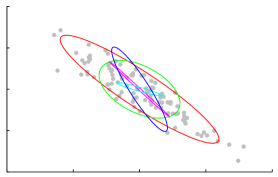
(a) Ellipses from ESS

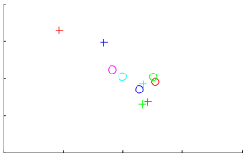
(b) Corresponding values of ${\bf x}$ and $\boldsymbol{\nu}$

Figure 1: Background points are drawn independently from a probability distribution, and five ellipses are created by elliptical slice sampling. The distribution in question is a two-dimensional multivariate Gaussian. In this example, the same distribution is used as the prior for elliptical slice sampling. (a) Shows the ellipses created by elliptical slice sampling. (b) Shows the values of ${\bf x}$ (depicted as ${{{\circ}}}$) and $\boldsymbol{\nu}$ (depicted as +) corresponding to each elliptical slice sampling update. The values of ${\bf x}$ and ${\boldsymbol{\nu}}$ with a given color correspond to the ellipse of the same color in (a).

Algorithm 1 Elliptical Slice Sampling Update

1:Current state ${\bf x}$, Gaussian parameters $\boldsymbol{\mu}$ and $\boldsymbol{\Sigma}$, log-likelihood function $\log L$

2:New state ${\bf x^{\prime}}$, with stationary distribution proportional to $\mathcal{N}({\bf x};\boldsymbol{\mu},\boldsymbol{\Sigma})L({\bf x})$

3:$\boldsymbol{\nu}\sim\mathcal{N}(\boldsymbol{\mu},\boldsymbol{\Sigma})$ $\triangleright$ Choose ellipse

4:$u\sim\textnormal{Uniform}[0,1]$

5:$\log y\leftarrow\log L({\bf x})+\log u$ $\triangleright$ Set log-likelihood threshold

6:$\theta\sim\textnormal{Uniform}[0,2\pi]$ $\triangleright$ Draw an initial proposal

7:$[\theta_{\min},\theta_{\max}]\leftarrow[\theta-2\pi,\theta]$ $\triangleright$ Define a bracket

8:${\bf x^{\prime}}\leftarrow({\bf x}-\boldsymbol{\mu})\cos\theta+(\boldsymbol{\nu}-\boldsymbol{\mu})\sin\theta+\boldsymbol{\mu}$

9:if $\log L({\bf x^{\prime}})>\log y$ then

10:     return ${\bf x^{\prime}}$ $\triangleright$ Accept

11:else$\triangleright$ Shrink the bracket and try a new point

12:     if $\theta<0$ then

13:         $\theta_{\min}\leftarrow\theta$

14:     else

15:         $\theta_{\max}\leftarrow\theta$      

16:     $\theta\sim\textnormal{Uniform}[\theta_{\min},\theta_{\max}]$

17:     goto 6

3 Generalized Elliptical Slice Sampling

In this section, we generalize elliptical slice sampling to handle arbitrary continuous distributions. We refer to this algorithm as generalized elliptical slice sampling (GESS). In this section, our target distribution will be a continuous distribution over $\mathbb{R}^{D}$ with density $\pi$. In practice, $\pi$ need not be normalized.

Our objective is to reframe our target distribution so that it can be efficiently sampled with elliptical slice sampling. One possible approach is to put $\pi$ in the form of Equation (1) by choosing some approximation $\mathcal{N}(\boldsymbol{\mu},\boldsymbol{\Sigma})$ to $\pi$ and writing

$$\pi({\bf x})=R({\bf x})\,\mathcal{N}({\bf x};\boldsymbol{\mu},\boldsymbol{\Sigma}),$$

where

$$R({\bf x})=\frac{\pi({\bf x})}{\mathcal{N}({\bf x};\boldsymbol{\mu},\boldsymbol{\Sigma})}$$

is the residual error of our approximation to the target density. Note that $\mathcal{N}({\bf x};\boldsymbol{\mu},\boldsymbol{\Sigma})$ is an approximation rather than a prior and that $R$ is not a likelihood function, but since the equation has the correct form, this representation enables us to use elliptical slice sampling.

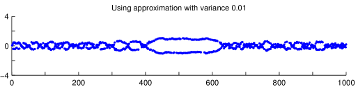
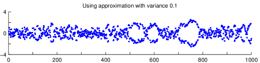
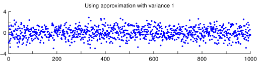
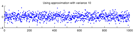
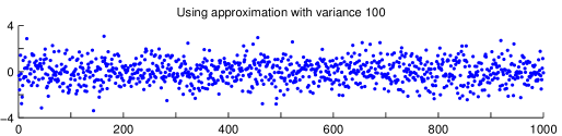
Figure 2: Samples are drawn from a Gaussian with zero mean and unit variance using elliptical slice sampling with various Gaussian approximations. These trace plots show how sampling behavior depends on how heavy the tails of the approximation are relative to how heavy the tails of the target distribution are. We plot one of every ten samples.

Applying elliptical slice sampling in this manner will produce a correct algorithm, but it may mix slowly in practice. Difficulties arise when the target distribution has much heavier tails than does the approximation. In such a situation, $R({\bf x})$ will increase rapidly as ${\bf x}$ moves away from the mean of the approximation. To illustrate this phenomenon, we use this approach with different approximations to draw samples from a Gaussian in one dimension with zero mean and unit variance. Trace plots are shown in Figure 2. The subplot corresponding to variance $0.01$ illustrates the problem. Since $R$ explodes as $|{\bf x}|$ gets large, the Markov chain is unlikely to move back toward the origin. On the other hand, the size of the ellipse is limited by a draw from the Gaussian approximation, which has low variance in this case, so the Markov chain is also unlikely to move away from the origin. The result is that the Markov chain sometimes gets stuck. In the subplot corresponding to variance $0.01$, this occurs between iterations $400$ and $630$.

In order to resolve this pathology and extend elliptical slice sampling to continuous distributions, we broaden the class of allowed approximations. To begin with, we express the density of the target distribution in the more general form

$$\pi({\bf x})\propto R({\bf x})\int\mathcal{N}({\bf x};\boldsymbol{\mu}(s),\boldsymbol{\Sigma}(s))\,\phi(\mathrm{d}s),$$ (3)

where the integral represents a scale-location mixture of Gaussians (which serves as an approximation to $\pi$), and where $\phi$ is a measure over the auxiliary parameter $s$. As before, $R$ is the residual error of the approximation. Here, $\phi$ can be chosen in a problem-specific way, and any residual error between $\pi$ and the approximation will be compensated for by $R$. Equation (3) is quite flexible. Below, we will choose the measure $\phi$ so as to make the approximation a multivariate $t$ distribution, but there are many other possibilities. For instance, taking $\phi$ to be a combination of point masses will make the approximation a discrete mixture of Gaussians.

Through Equation (3), we can view $\pi({\bf x})$ as the marginal density of an augmented joint distribution over ${\bf x}$ and $s$. Using $\lambda$ to denote the density of $\phi$ with respect to the base measure over $s$ (this is fully general because we have control over the choice of base measure), we can write

$$p({\bf x},s)=R({\bf x})\,\mathcal{N}({\bf x};\boldsymbol{\mu}(s),\boldsymbol{\Sigma}(s))\,\lambda(s).$$

Therefore, to sample $\pi$, it suffices to sample ${\bf x}$ and $s$ jointly and then to marginalize out the $s$ coordinate (by simply dropping the $s$ coordinate). We update these components alternately so as to leave invariant the distributions

$$p({\bf x}\,|\,s)\propto R({\bf x})\,\mathcal{N}({\bf x};\boldsymbol{\mu}(s),\boldsymbol{\Sigma}(s))$$ (4)

and

$$p(s\,|\,{\bf x})\propto\mathcal{N}({\bf x};\boldsymbol{\mu}(s),\boldsymbol{\Sigma}(s))\,\lambda(s).$$ (5)

Equation (4) has the correct form for elliptical slice sampling and can be updated according to Algorithm 1. Equation (5) can be updated using any valid Markov transition operator.

We now focus on a particular case in which the update corresponding to Equation (5) is easy to simulate and in which we can make the tails as heavy as we desire, so as to control the behavior of $R$. A simple and convenient choice is for the scale-location mixture to yield a multivariate $t$ distribution with degrees-of-freedom parameter $\nu$:

$$\mathcal{T}_{\nu}({\bf x};\boldsymbol{\mu},\boldsymbol{\Sigma})=\int_{0}^{\infty}\textnormal{IG}(s;\tfrac{\nu}{2},\tfrac{\nu}{2})\,\mathcal{N}({\bf x};\boldsymbol{\mu},s\boldsymbol{\Sigma})\,\mathrm{d}s,$$

where $\lambda$ becomes the density function of an inverse-gamma distribution:

$$\text{IG}(s;\alpha,\beta)=\frac{\beta^{\alpha}}{\Gamma(\alpha)}s^{-\alpha-1}e^{-\beta/s}.$$

Here $s$ is a positive real-valued scale parameter. Now, in the update $p(s\,|\,{\bf x})$, we observe that the inverse-gamma distribution acts as a conjugate prior (whose “prior” parameters are $\alpha=\frac{\nu}{2}$ and $\beta=\frac{\nu}{2}$), so

$$p(s\,|\,{\bf x})=\textnormal{IG}(s;\alpha^{\prime},\beta^{\prime})$$

with parameters

$$\alpha^{\prime} = \frac{D+\nu}{2}\,\,\,\,\,\,\,\,\text{and}$$ (6)

$$\beta^{\prime} = \frac{1}{2}(\nu+({\bf x}-\boldsymbol{\mu})^{\sf T}\boldsymbol{\Sigma}^{-1}({\bf x}-\boldsymbol{\mu})).$$ (7)

We can draw independent samples from this distribution (Devroye, 1986).

Combining these update steps, we define the transition operator $S({\bf x}\to{\bf x^{\prime}};\nu,\boldsymbol{\mu},\boldsymbol{\Sigma})$ to be the one which draws $s\sim\textnormal{IG}(s;\alpha^{\prime},\beta^{\prime})$, with $\alpha^{\prime}$ and $\beta^{\prime}$ as described in Equations (6) and (7), and then uses elliptical slice sampling to update ${\bf x}$ so as to leave invariant the distribution defined in Equation (4), where $\boldsymbol{\mu}(s)=\boldsymbol{\mu}$ and $\boldsymbol{\Sigma}(s)=s\boldsymbol{\Sigma}$. From the above discussion, it follows that the stationary distribution of $S({\bf x}\to{\bf x^{\prime}};\nu,\boldsymbol{\mu},\boldsymbol{\Sigma})$ is $\pi$. Figure 3 illustrates this transition operator.

Algorithm 2 Generalized Elliptical Slice Sampling Update

1:Current state ${\bf x}$, multivariate $t$ parameters $\nu,\boldsymbol{\mu},\boldsymbol{\Sigma}$, dimension $D$, a routine ESS that performs an elliptical slice sampling update

2:New state ${\bf x^{\prime}}$

3:$\alpha^{\prime}\leftarrow\frac{D+\nu}{2}$

4:$\beta^{\prime}\leftarrow\frac{1}{2}(\nu+({\bf x}-\boldsymbol{\mu})^{\sf T}\boldsymbol{\Sigma}^{-1}({\bf x}-\boldsymbol{\mu}))$

5:$s\sim\textnormal{IG}(\alpha^{\prime},\beta^{\prime})$

6:$\log L\leftarrow\log\pi-\log\mathcal{T}$ $\triangleright$ $\mathcal{T}$ is the density of a multivariate $t$ with parameters $\nu,\boldsymbol{\mu},\boldsymbol{\Sigma}$

7:${\bf x^{\prime}}\leftarrow\textnormal{ESS}({\bf x},\boldsymbol{\mu},s\boldsymbol{\Sigma},\log L)$

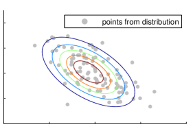
(a) Multivariate $t$ contours

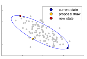
(b) Example GESS update

Figure 3: The gray points were drawn independently from a two-dimensional Gaussian to show the mode and shape of the corresponding density function. (a) Shows the contours of a multivariate $t$ approximation to this distribution. (b) Shows a sample update step using the transition operator $S({\bf x}\to~{}{\bf x^{\prime}};\nu,\boldsymbol{\mu},\boldsymbol{\Sigma})$. The blue point represents the current state. The yellow point defines an ellipse and is drawn from the Gaussian distribution corresponding to the scale $s$ drawn from the appropriate inverse-gamma distribution. The red point corresponds to the new state and is sampled from the given ellipse.

4 Building the Approximation with Parallelism

Up to this point, we have not described how to choose the multivariate $t$ parameters $\nu$, $\boldsymbol{\mu}$, and $\boldsymbol{\Sigma}$. These choices can be made in many ways. For instance, we may choose the maximum likelihood parameters given samples collected during a burn in period, we may build a Laplace approximation to the mode of the distribution, or we may use variational approaches. Note that this algorithm is valid regardless of the particular choice we make here. In this section, we discuss a convenient way to use parallelism to dynamically choose these parameters without requiring tuning runs or exploratory analysis of the distribution. This method creates a large number of parallel chains, each producing samples from $\pi$, and it divides them into two groups. The need for two groups of Markov chains is not immediately obvious, so we motivate our approach by first discussing two simpler algorithms that fail in different ways.

4.1 Naïve Approaches

We begin with a collection of $K$ parallel chains. Let ${\mathcal{X}~{}=~{}\{{\bf x}_{1},\ldots,{\bf x}_{K}\}}$ denote the current states of the chains. We observe that $\mathcal{X}$ may contain a lot of information about the shape of the target distribution. We would like to define a transition operator $Q(\mathcal{X}\to\mathcal{X}^{\prime})$ that uses this information to intelligently choose the multivariate $t$ parameters $\nu$, $\boldsymbol{\mu}$, and $\boldsymbol{\Sigma}$ and then uses these parameters to update each ${\bf x}_{k}$ via generalized elliptical slice sampling. Additionally, we would like $Q$ to have two properties. First, each ${\bf x}_{k}$ should have the marginal stationary distribution $\pi$. Second, we should be able to parallelize the update of $\mathcal{X}$ over $K$ cores.

Here we describe two simple approaches for parallelizing generalized elliptical slice sampling, each of which lacks one of the desired properties. The first approach begins with $K$ parallel Markov chains, and it requires a procedure for choosing the multivariate $t$ parameters given $\mathcal{X}$ (for example, maximum likelihood estimation). In this setup, $Q$ uses this procedure to determine the multivariate $t$ parameters $\nu_{\mathcal{X}}$, $\boldsymbol{\mu}_{\mathcal{X}}$, $\boldsymbol{\Sigma}_{\mathcal{X}}$ from $\mathcal{X}$ and then applies $S({\bf x}\to{\bf x^{\prime}};\nu_{\mathcal{X}},\boldsymbol{\mu}_{\mathcal{X}},\boldsymbol{\Sigma}_{\mathcal{X}})$ to each ${\bf x}_{k}$ individually. These updates can be performed in parallel, but the variables ${\bf x}_{k}$ no longer have the correct marginal distributions because of the coupling between the chains introduced by the approximation (this update violates detailed balance).

A second approach creates a valid MCMC method by including the multivariate $t$ parameters in a joint distribution

$$p(\mathcal{X},\nu,\boldsymbol{\mu},\boldsymbol{\Sigma})=p(\nu,\boldsymbol{\mu},\boldsymbol{\Sigma}\,|\,\mathcal{X})\left[\prod_{k=1}^{K}\pi({\bf x}_{k})\right].$$ (8)

Note that in Equation (8), each ${\bf x}_{k}$ has marginal distribution $\pi$. We can sample this joint distribution by alternately updating the variables and the multivariate $t$ parameters so as to leave invariant the conditional distributions $p(\mathcal{X}\,|\,\nu,\boldsymbol{\mu},\boldsymbol{\Sigma})$ and $p(\nu,\boldsymbol{\mu},\boldsymbol{\Sigma}\,|\,\mathcal{X})$. Ideally, we would like to update the collection $\mathcal{X}$ by updating each ${\bf x}_{k}$ in parallel. However, we cannot easily parallelize the update in this formulation because of the factor of $p(\nu,\boldsymbol{\mu},\boldsymbol{\Sigma}\,|\,\mathcal{X})$, which nontrivially couples the chains.

4.2 The Two-Group Approach

Our proposed method creates a transition operator $Q$ that satisfies both of the desired properties. That is, each ${\bf x}_{k}$ has marginal distribution $\pi$, and the update can be efficiently parallelized. This method circumvents the problems of the previous approaches by maintaining two groups of Markov chains and using each group to choose multivariate $t$ parameters to update the other group. Let $\mathcal{X}=\{{\bf x}_{1},\ldots,{\bf x}_{K_{1}}\}$ and $\mathcal{Y}=\{{\bf y}_{1},\ldots,{\bf y}_{K_{2}}\}$ denote the states of the Markov chains in these two groups (in practice, we set $K_{1}=K_{2}=K$, where $K$ is the number of available cores). The stationary distribution of the collection is

$$\Pi(\mathcal{X},\mathcal{Y})=\Pi_{1}(\mathcal{X})\Pi_{2}(\mathcal{Y})=\left[\prod_{k=1}^{K_{1}}\pi({\bf x}_{k})\right]\left[\prod_{k=1}^{K_{2}}\pi({\bf y}_{k})\right].$$

By simulating a Markov chain which leaves this product distribution invariant, this method generates samples from the target distribution. Our Markov chain is based on a transition operator, $Q$, defined in two parts. The first part of the transition operator, $Q_{1}$, uses $\mathcal{Y}$ to determine parameters $\nu_{\mathcal{Y}}$, $\boldsymbol{\mu}_{\mathcal{Y}}$, and $\boldsymbol{\Sigma}_{\mathcal{Y}}$. It then uses these parameters to update $\mathcal{X}$. The second part of the transition operator, $Q_{2}$, uses $\mathcal{X}$ to determine parameters $\nu_{\mathcal{X}}$, $\boldsymbol{\mu}_{\mathcal{X}}$, and $\boldsymbol{\Sigma}_{\mathcal{X}}$. It then uses these parameters to update $\mathcal{Y}$. The transition operator $Q$ is the composition of $Q_{1}$ and $Q_{2}$. The idea of maintaining a group of Markov chains and updating the states of some Markov chains based on the states of other Markov chains has been discussed in the literature before. For example, see Zhang and Sutton (2011); Gilks et al. (1994).

In order to make these descriptions more precise, we define $Q_{1}$ as follows. First, we specify a procedure for choosing the multivariate $t$ parameters given the population $\mathcal{Y}$. We use an extension of the expectation-maximization algorithm (Liu and Rubin, 1995) to choose the maximum-likelihood multivariate $t$ parameters given the data $\mathcal{Y}$. The details of this algorithm are described in Algorithm 4 in the Appendix. More concretely, we choose

$$\nu_{\mathcal{Y}},\boldsymbol{\mu}_{\mathcal{Y}},\boldsymbol{\Sigma}_{\mathcal{Y}}=\operatornamewithlimits{arg\,max}_{\nu,\boldsymbol{\mu},\boldsymbol{\Sigma}}\prod_{k=1}^{K_{2}}\mathcal{T}_{\nu}({\bf y}_{k}\,;\,\boldsymbol{\mu},\boldsymbol{\Sigma}).$$

After choosing $\nu_{\mathcal{Y}}$, $\boldsymbol{\mu}_{\mathcal{Y}}$, and $\boldsymbol{\Sigma}_{\mathcal{Y}}$ in this manner, we update $\mathcal{X}$ by applying the transition operator $S({\bf x}\to~{}{\bf x^{\prime}};\nu_{\mathcal{Y}},\boldsymbol{\mu}_{\mathcal{Y}},\boldsymbol{\Sigma}_{\mathcal{Y}})$ to each ${\bf x}_{k}\in\mathcal{X}$ in parallel. The operator $Q_{2}$ is defined analogously.

Algorithm 3 Building the Approximation Using Parallelism

1:Two groups of states $\mathcal{X}=\{{\bf x}_{1},\ldots,{\bf x}_{K_{1}}\}$ and $\mathcal{Y}=\{{\bf y}_{1},\ldots,{\bf y}_{K_{2}}\}$, a subroutine FIT-MVT which takes data and returns the maximum-likelihood $t$ parameters, a subroutine GESS which performs a generalized elliptical slice sampling update

2:Updated groups $\mathcal{X}^{\prime}$ and $\mathcal{Y}^{\prime}$

3:$\nu,\boldsymbol{\mu},\boldsymbol{\Sigma}\leftarrow\textnormal{FIT-MVT}(\mathcal{Y})$

4:for all ${\bf x}_{k}\in\mathcal{X}$ do

5:     ${\bf x}_{k}^{\prime}=\textnormal{GESS}({\bf x}_{k},\nu,\boldsymbol{\mu},\boldsymbol{\Sigma})$

6:$\mathcal{X}^{\prime}\leftarrow\{{\bf x}_{1}^{\prime},\ldots,{\bf x}_{K_{1}}^{\prime}\}$

7:$\nu,\boldsymbol{\mu},\boldsymbol{\Sigma}\leftarrow\textnormal{FIT-MVT}(\mathcal{X}^{\prime})$

8:for all ${\bf y}_{k}\in\mathcal{Y}$ do

9:     ${\bf y}_{k}^{\prime}=\textnormal{GESS}({\bf y}_{k},\nu,\boldsymbol{\mu},\boldsymbol{\Sigma})$

10:$\mathcal{Y}^{\prime}\leftarrow\{{\bf y}_{1}^{\prime},\ldots,{\bf y}_{K_{2}}^{\prime}\}$

In the case where the number of chains in the collection $\mathcal{Y}$ is less than or close to the dimension of the distribution, the particular algorithm that we use to choose the parameters (Liu and Rubin, 1995) may not converge quickly (or at all). Suppose we are in the setting where $K<2D$. In this situation, we can perform a regularized estimate of the parameters. We describe this procedure below. The choice $K<2D$ probably overestimates the regime in which the algorithm for fitting the parameters performs poorly. The particular algorithm that we use appears to work well as long as $K\geq D$.

Let $\bar{\bf y}$ be the mean of $\mathcal{Y}$, and let $\{{\bf v}_{1},\ldots,{\bf v}_{J}\}$ be the first ${J}$ principal components of the set $\{{\bf y}_{1}-\bar{\bf y},\ldots,{\bf y}_{K}-\bar{\bf y}\}$, where ${J}=\lfloor\tfrac{K}{2}\rfloor$, and let $V=\textnormal{span}({\bf v}_{1},\ldots,{\bf v}_{J})$. Let ${\bf A}$ be the $D\times{J}$ matrix defined by ${\bf A}{\bf e}_{j}={\bf v}_{j}$, where ${\bf e}_{j}$ is the $j$th standard basis vector in $\mathbb{R}^{J}$. This map identifies $\mathbb{R}^{J}$ with $V$.

Let the set $\hat{\mathcal{Y}}$ consist of the projections of the elements of $\mathcal{Y}$ onto $\mathbb{R}^{J}$ by $\hat{\bf y}_{k}={\bf A}^{\mathsf{T}}{\bf y}_{k}$. Using the algorithm from Liu and Rubin (1995), fit the multivariate $t$ parameters $\nu_{\hat{\mathcal{Y}}}$, $\boldsymbol{\mu}_{\hat{\mathcal{Y}}}$ and, $\boldsymbol{\Sigma}_{\hat{\mathcal{Y}}}$ to $\hat{\mathcal{Y}}$. At this point, we have constructed a ${J}$-dimensional multivariate $t$ distribution, but we would like a $D$-dimensional one. We construct the desired distribution by rotating back to the original space. Concretely, we can set

$$\nu_{\mathcal{Y}} = \nu_{\hat{\mathcal{Y}}}$$

$$\boldsymbol{\mu}_{\mathcal{Y}} = {\bf A}\,\boldsymbol{\mu}_{\hat{\mathcal{Y}}}+\bar{{\bf y}}$$

$$\boldsymbol{\Sigma}_{\mathcal{Y}} = {\bf A}\,\boldsymbol{\Sigma}_{\hat{\mathcal{Y}}}\,{\bf A}^{\mathsf{T}}+\epsilon\,{\bf I}_{D},$$

where ${\bf I}_{D}$ is the $D\times D$ identity matrix and $\epsilon$ is the median entry on the diagonal of $\boldsymbol{\Sigma}_{\hat{\mathcal{Y}}}$. We add a scaled identity matrix to the covariance parameter to avoid producing a degenerate distribution. The choice of $\epsilon$ is based on intuition about typical values of the variance of $\pi$ in the directions orthogonal to $V$.

We emphasize that the nature of the procedure for fitting a multivariate $t$ distribution to some points is not important to our algorithm. One could devise more sophisticated approaches drawing on ideas from the literature on high-dimensional covariance estimation, see Ravikumar et al. (2011) for instance, but we merely choose a simple idea that seems to work in practice. Since our default choice (if there are at least $2D$ chains, then choose the maximum-likelihood parameters, otherwise project to a lower dimension, choose the maximum-likelihood parameters, and then pad the diagonal of the covariance parameter) works well, the fact that one could design a more sophisticated procedure does not compromise the tuning-free nature of our algorithm.

4.3 Correctness

To establish the correctness of our algorithm, we treat the collection of chains as a single aggregate Markov chain, and we show that this aggregate Markov chain with transition operator $Q$ correctly samples from the product distribution $\Pi$.

We wish to show that $Q_{1}$ and $Q_{2}$ preserve the invariant distributions $\Pi_{1}$ and $\Pi_{2}$ respectively. As the two cases are identical, we consider only the first. We have

$$\int\Pi_{1}(\mathcal{X})\,Q_{1}(\mathcal{X}\to\mathcal{X}^{\prime})\,\mathrm{d}\mathcal{X} = \int\Pi_{1}(\mathcal{X})\,Q_{1}(\mathcal{X}\to\mathcal{X}^{\prime}\,|\,\nu_{\mathcal{Y}},\boldsymbol{\mu}_{\mathcal{Y}},\boldsymbol{\Sigma}_{\mathcal{Y}})\,\mathrm{d}\mathcal{X}$$

$$= \prod_{k=1}^{K_{1}}\left[\int\pi({\bf x}_{k})\,S({\bf x}_{k}\to{\bf x}_{k}^{\prime};\nu_{\mathcal{Y}},\boldsymbol{\mu}_{\mathcal{Y}},\boldsymbol{\Sigma}_{\mathcal{Y}})\,\mathrm{d}{\bf x}_{k}\right]$$

$$= \Pi_{1}(\mathcal{X}^{\prime}).$$

The last equality uses the fact that $\pi$ is the stationary distribution of $S({\bf x}\to{\bf x^{\prime}};\nu_{\mathcal{Y}},\boldsymbol{\mu}_{\mathcal{Y}},\boldsymbol{\Sigma}_{\mathcal{Y}})$, so we see that $Q$ leaves the desired product distribution invariant.

Within a single chain, elliptical slice sampling has a nonzero probability of transitioning to any region that has nonzero probability under the posterior, as described by Murray et al. (2010). The transition operator $Q$ updates the chains in a given group independently of one another. Therefore $Q$ has a nonzero probability of transitioning to any region that has nonzero probability under the product distribution. It follows that the transition operator is both irreducible and aperiodic. These conditions together ensure that this Markov transition operator has a unique invariant distribution, namely $\Pi$, and that the distribution over the state of the Markov chain created from this transition operator will converge to this invariant distribution (Roberts and Rosenthal, 2004). It follows that, in the limit, samples derived from the repeated application of $Q$ will be drawn from the desired distribution.

4.4 Cost and Complexity

There is a cost to the construction of the multivariate $t$ approximation. Although the user has some flexibility in the choice of $t$ parameters, we fit them with the iterative algorithm described by Liu and Rubin (1995) and in Algorithm 4 of the Appendix. Let $D$ be the dimension of the distribution and let $K$ be the number of parallel chains. Then the complexity of each iteration is $O(D^{3}K)$, which comes from the fact that we invert a $D\times D$ matrix for each of the $K$ chains. Empirically, Algorithm 4 appears to converge in a small number of iterations when the number of parallel Markov chains in each group exceeds the dimension of the distribution. As described in the next section, this cost can be amortized by reusing the same approximation for multiple updates. On the challenging distributions that most interest us, the cost of constructing the approximation (when amortized in this manner), will be negligible compared to the cost of evaluating the density function.

An additional concern is the overhead from sharing information between chains. The chains must communicate in order to build a multivariate $t$ approximation, and so the updates must be synchronized. Since elliptical slice sampling requires a variable amount of time, updating the different chains will take different amounts of time, and the faster chains may end up waiting for the slower ones. We can mitigate this cost by performing multiple updates between such periods of information sharing. In this manner, we can perform as much computation as we want between synchronizations without compromising the validity of the algorithm. As we increase the number of updates performed between synchronizations, the fraction of time spent waiting will diminish.

The time measured in our experiments is wall-clock time, which includes the overhead from constructing the approximation and from synchronizing the chains.

4.5 Reusing the Approximation

Here we explain that reusing the same approximation is valid. To illustrate this point, let the transition operators $Q_{1}$ and $Q_{2}$ be defined as before. In our description of the algorithm, we defined the transition operator $Q$ as the composition ${Q=Q_{2}Q_{1}}$. However, both $Q_{1}$ and $Q_{2}$ preserve the desired product distribution, so we may use any transition operator of the form ${Q=Q_{2}^{r_{2}}Q_{1}^{r_{1}}}$, where this notation indicates that we first apply $Q_{1}$ for $r_{1}$ rounds and then we apply $Q_{2}$ for $r_{2}$ rounds. As long as $r_{2},r_{1}\geq 1$, the composite transition operator is ergodic. When we apply $Q_{1}$ multiple times in a row, the states $\mathcal{Y}$ do not change, so if $Q_{1}$ computes $\nu_{\mathcal{Y}}$, $\boldsymbol{\mu}_{\mathcal{Y}}$, and $\boldsymbol{\Sigma}_{\mathcal{Y}}$ deterministically from $\mathcal{Y}$, then we need only compute these values once. Reusing the approximation works even if $Q_{1}$ samples $\nu_{\mathcal{Y}}$, $\boldsymbol{\mu}_{\mathcal{Y}}$, and $\boldsymbol{\Sigma}_{\mathcal{Y}}$ from some distribution. In this case, we can model the randomness by introducing a separate variable $r_{\mathcal{Y}}$ in the Markov chain, and letting $Q_{1}$ compute $\nu_{\mathcal{Y}}$, $\boldsymbol{\mu}_{\mathcal{Y}}$, and $\boldsymbol{\Sigma}_{\mathcal{Y}}$ deterministically from $\mathcal{Y}$ and $r_{\mathcal{Y}}$.

Our algorithm maintains two collections of Markov chains, one of which will always be idle. Therefore, each collection can take advantage of all available cores. Given $K$ cores, it makes sense to use two collections of $K$ Markov chains. In general, it seems to be a good idea to sample equally from both collections so that the chains in both collections burn in.

To motivate reusing the approximation, we demonstrate the effect of reusing the approximation for different numbers of iterations on a Gaussian distribution in $100$ dimensions (the same one that we use in Section 6.2). For each value of $i$ from $1$ to $4$, we sample this distribution for $10^{4}$ iterations and we reuse each approximation for $10^{i}$ iterations. We show plots of the running time of GESS and the convergence of the approximation for different values of $i$. Figure 4 shows how the amount of time required by GESS changes as we vary $i$, and how the covariance matrix parameter of the fitted multivariate $t$ approximation changes over time for the different values of $i$. We summarize the covariance matrix parameter by its trace $\text{tr}(\boldsymbol{\Sigma})$. The figure shows that increasing the number of iterations for which we reuse the approximation can dramatically reduce the amount of time required by GESS. It also shows that if we rebuild the approximation frequently, the approximation will settle on a reasonable approximation in fewer iterations. However, there is little difference between rebuilding the approximation every $10$ iterations versus every $100$ iterations (in terms of the number of iterations required), while there is a dramatic difference in the time required.

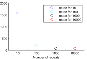
(a) Durations of GESS (seconds)

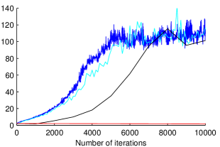
(b) Plots of $\text{tr}(\boldsymbol{\Sigma})$

Figure 4: We used GESS to sample a multivariate Gaussian distribution in $100$ dimensions for $10^{4}$ iterations. We repeated this procedure four times, reusing the approximation for $10^{1}$, $10^{2}$, $10^{3}$, and $10^{4}$ iterations. (a) Shows the durations (in seconds) of the sampling procedures as we varied the number of iterations for which we reused the approximation. (b) Shows how $\text{tr}(\boldsymbol{\Sigma})$ changes over time in the four different settings.

5 Related Work

Our work uses updates on a product distribution in the style of Adaptive Direction Sampling (Gilks et al., 1994), which has inspired a large literature of related methods. The closest research to our work makes use of slice-sampling based updates of product distributions along straight-line directions chosen by sampling pairs of points (MacKay, 2003; Ter Braak, 2006). The work on elliptical slice sampling suggests that in high dimensions larger steps can be taken along curved trajectories, given an appropriate Gaussian fit. Using closed ellipses also removes the need to set an initial step size or to build a bracket.

The recent affine invariant ensemble sampler (Goodman and Weare, 2010) also uses Gaussian fits to a population, in that case to make Metropolis proposals. Our work differs by using a scale-mixture of Gaussians and elliptical slice sampling to perform updates on a variety of scales with self-adjusting step-sizes. Rather than updating each member of the population in sequence, our approach splits the population into two groups and allows the members of each group to be updated in parallel.

Population MCMC with parallel tempering (Friel and Pettitt, 2008) is another parallel sampling approach that involves sampling from a product distribution. It uses separate chains to sample a sequence of distributions interpolating between the target distribution and a simpler distribution. The different chains regularly swap states to encourage mixing. In this setting, samples are generated only from a single chain, and all of the others are auxiliary. However, some tasks such as computing model evidence can make use of samples from all of the chains (Friel and Pettitt, 2008).

Recent work on Hamiltonian Monte Carlo has attempted to reduce the tuning burden (Hoffman and Gelman, 2014). A user friendly tool that combines this work with a software stack supporting automatic differentiation is under development (Stan Development Team, 2012). We feel that this alternative line of work demonstrates the interest in more practical MCMC algorithms applicable to a variety of continuous-valued parameter spaces and is very promising. Our complementary approach introduces simpler algorithms with fewer technical software requirements. In addition, our two-population approach to parallelization could be applied with whichever methods become dominant in the future.

6 Experiments

In this section, we compare Algorithm 3 with other parallel MCMC algorithms by measuring how quickly the Markov chains mix on a number of different distributions. Second, we compare how the performance of Algorithm 3 scales with the dimension of the target distribution, the number of cores used, and the number of chains used per core.

These experiments were run on an EC2 cluster with $5$ nodes, each with two eight-core Intel Xeon E5-2670 CPUs. We implement all algorithms in Python, using the IPython environment (Pérez and Granger, 2007) for parallelism.

6.1 Comparing Mixing

We empirically compare the mixing of the parallel MCMC samplers on seven distributions. We quantify their mixing by comparing the effective number of samples produced by each method. This quantity can be approximated as the product of the number of chains with the effective number of samples from the product distribution. We estimate the effective number of samples from the product distribution by computing the effective number of samples from its sequence of log likelihoods. We compute effective sample size using R-CODA (Plummer et al., 2006), and we compare the results using two metrics: effective samples per second and effective samples per density function evaluation (in the case of Hamiltonian Monte Carlo, we count gradient evaluations as density function evaluations).

In each experiment, we run each algorithm with $100$ parallel chains. Unless otherwise noted, we burn in for $10^{4}$ iterations and sample for $10^{5}$ iterations. We run five trials for each experiment to estimate variability.

Figure 5 shows the average effective number of samples, with error bars, according to the two different metrics. Bars are omitted where the sequence of aggregate log likelihoods did not converge according to the Geweke convergence diagnostic (Geweke, 1992). We diagnose this using the tool from R-CODA (Plummer et al., 2006).

6.1.1 Samplers Considered

We compare generalized elliptical slice sampling (GESS) with parallel versions of several different sampling algorithms.

First, we consider random-direction slice sampling (RDSS) (MacKay, 2003) and coordinate-wise slice sampling (CWSS) (Neal, 2003). These are variants of slice sampling which differ in their choice of direction (a random direction versus a random axis-aligned direction) in which to sample. RDSS is rotation invariant like GESS, but CWSS is not.

In addition, we compare to a simple Metropolis–Hastings (MH) (Metropolis et al., 1953) algorithm whose proposal distribution is a spherical Gaussian centered on the current state. A tuning period is used to adjust the MH step size so that the acceptance ratio is as close as possible to the value $0.234$, which is optimal in some settings (Roberts and Rosenthal, 1998). This tuning is done independently for each chain. We also compare to an adaptive MCMC (AMH) algorithm following the approach in Roberts and Rosenthal (2006) in which the covariance of a Metropolis–Hastings proposal is adapted to the history of the “Markov” chain.

We also compare to the No-U-Turn sampler (Hoffman and Gelman, 2014), which is an implementation of Hamiltonian Monte Carlo (HMC) combined with procedures to automatically tune the step size parameter and the number of steps parameter. Due to the large number of function evaluations per sample required by HMC, we run HMC for a factor of $10$ or $100$ fewer iterations in order to make the algorithms roughly comparable in terms of wall-clock time. Though we include the comparisons, we do not view HMC as a perfectly comparable algorithm due to its requirement that the density function of the target distribution be differentiable. Though the target distribution is often differentiable in principle, there are many practical situations in which the gradient is difficult to access, either by manual computation or by automatic differentiation, possibly because evaluating the density function requires running a complicated black-box subroutine. For instance, in computer vision problems, evaluating the likelihood function may require rendering an image or running graph cuts. See Tarlow and Adams (2012) or Lang and Hogg (2012) for examples.

We compare to parallel tempering (PT) (Friel and Pettitt, 2008), using each Markov chain to sample the distribution at a different temperature (if the target distribution has density $\pi({\bf x})$, then the distribution “at temperature $t$” has density proportional to $\pi({\bf x})^{1/t}$) and swapping states between the Markov chains at regular intervals. Samples from the target distribution are produced by only one of the chains. Using PT requires the practitioner to pick a temperature schedule, and doing so often requires a significant amount of experimentation (Neal, 2001). We follow the practice of Friel and Pettitt (2008) and use a geometric temperature schedule. As with HMC, we do not view PT as entirely comparable in the absence of an automatic and principled way to choose the temperatures of the different Markov chains. One of the main goals of GESS is to provide a black-box MCMC algorithm that imposes as few restrictions on the target distribution as possible and that requires no expertise or experimentation on the part of the user.

6.1.2 Distributions

In this section, we describe the different distributions that we use to compare the mixing of our samplers.

Funnel: A ten-dimensional funnel-shaped distribution described in Neal (2003). The first coordinate is distributed normally with mean zero and variance nine. Conditioned on the first coordinate $v$, the remaining coordinates are independent identically-distributed normal random variables with mean zero and variance $e^{v}$. In this experiment, we initialize each Markov chain from a spherical multivariate Gaussian centered on the origin.

Gaussian Mixture: An eight-component mixture of Gaussians in eight dimensions. Each component is a spherical Gaussian with unit variance. The components are distributed uniformly at random within a hypercube of edge length four. In this experiment, we initialize each Markov chain from a spherical multivariate Gaussian centered on the origin.

Breast Cancer: The posterior density of a linear logistic regression model for a binary classification problem with thirty explanatory variables (thirty-one dimensions) using the Breast Cancer Wisconsin data set (Street et al., 1993). The data set consists of $569$ data points. We scale the data so that each coordinate has unit variance, and we place zero-mean Gaussian priors with variance $100$ on each of the regression coefficients. In this experiment, we initialize each Markov chain from a spherical multivariate Gaussian centered on the origin.

German Credit: The posterior density of a linear logistic regression model for a binary classification problem with twenty-four explanatory variables (twenty-five dimensions) from the UCI repository (Frank and Asuncion, 2010). The data set consists of $1000$ data points. We scale the data so that each coordinate has unit variance, and we place zero-mean Gaussian priors with variance $100$ on each of the regression coefficients. In this experiment, we initialize each Markov chain from a spherical multivariate Gaussian centered on the origin.

Stochastic Volatility: The posterior density of a simple stochastic volatility model fit to synthetic data in fifty-one dimensions. This distribution is a smaller version of a distribution described in Hoffman and Gelman (2014). In this experiment, we burn-in for $10^{5}$ iterations and sample for $10^{5}$ iterations. We initialize each Markov chain from a spherical multivariate Gaussian centered on the origin and we take the absolute value of the first parameter, which is constrained to be positive.

Ionosphere: The posterior density on covariance hyperparameters for Gaussian process regression applied to the Ionosphere data set (Sigillito et al., 1989). We use a squared exponential kernel with thirty-four length-scale hyperparameters and $100$ data points. We place exponential priors with rate $0.1$ on the length-scale hyperparameters. In this experiment, we burn-in for $10^{4}$ iterations and sample for $10^{4}$ iterations. We initialize each Markov chain from a spherical multivariate Gaussian centered on the vector $(1,\ldots,1)^{\mathsf{T}}$.

SNP Covariates: The posterior density of the parameters of a generative model for gene expression levels simulated in thirty-eight dimensions using actual genomic sequences from $480$ individuals for covariate data (Engelhardt and Adams, 2014). In this experiment, we burn-in for $2000$ iterations and sample for $10^{4}$ iterations. We initialize each Markov chain from a spherical multivariate Gaussian centered on the origin and we take the absolute value of the first three parameters, which are constrained to be positive.

6.1.3 Mixing Results

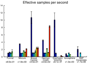
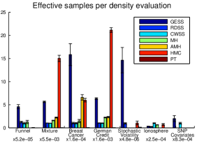
Figure 5: The results of experimental comparisons of seven parallel MCMC methods on seven distributions. Each figure shows seven groups of bars, (one for each distribution) and the vertical axis shows the effective number of samples per unit cost. Error bars are included. Bars are omitted where the method failed to converge according to the Geweke diagnostic (Geweke, 1992). The costs are per second (left) and per density function evaluation (right). Mean and standard error for five runs are shown. Each group of bars has been rescaled for readability: the number beneath each group gives the effective samples corresponding to CWSS, which always has height one.

The results of the mixing experiments are shown in Figure 5. For the most part, GESS sampled more effectively than the other algorithms according to both metrics. The poor performance of PT can be attributed to the fact that PT only produces samples from one of its chains, unlike the other algorithms, which produce samples from $100$ chains. HMC also performed well, although it failed to converge on the SNP Covariates distribution. The density function of this particular distribution is only piecewise continuous, with the discontinuities arising from thresholding in the model. In this case, the gradient and curvature largely reflect the prior, whereas the likelihood mostly manifests itself in the discontinuities of the distribution.

One reason for the rapid mixing of GESS is that GESS performs well even on highly-skewed distributions. RDSS, CWSS, MH, and PT propose steps in uninformed directions, the vast majority of which lead away from the region of high density. As a result, these algorithms take very small steps, causing successive states to be highly correlated. In the case of GESS, the multivariate $t$ approximation builds information about the global shape of the distribution (including skew) into the transition operator. As a consequence, the Markov chain can take long steps along the length of the distribution, allowing the Markov chain to mix much more rapidly. Skewed distributions can arise as a result of the user not knowing the relative length scales of the parameters or as a result of redundancy in the parameterization. Therefore, the ability to perform well on such distributions is frequently relevant.

These results show that a multivariate $t$ approximation to the target distribution provides enough information to greatly speed up the mixing of the sampler and that this information can be used to improve the convergence of the sampler. These improvements occur on top of the performance gain from using parallelism.

6.2 Scaling the Number of Cores

$D=50$	$K=C$	$K=2C$	$K=3C$	$K=4C$	$K=5C$
$C=20$	${\color[rgb]{0,0,1}\scriptstyle{10^{-0.5}\pm 10^{-0.4}}}$	${\color[rgb]{0,0,1}\scriptstyle{10^{-1.2}\pm 10^{-1.5}}}$	${\color[rgb]{0,0,1}\scriptstyle{10^{-1.5}\pm 10^{-1.8}}}$	${\color[rgb]{0,0,1}\scriptstyle{10^{-1.7}\pm 10^{-1.8}}}$	${\color[rgb]{0,0,1}\scriptstyle{10^{-1.6}\pm 10^{-1.6}}}$
$C=40$	${\color[rgb]{0,0,1}\scriptstyle{10^{-0.8}\pm 10^{-0.9}}}$	${\color[rgb]{0,0,1}\scriptstyle{10^{-2.6}\pm 10^{-2.6}}}$	${\color[rgb]{0,0,1}\scriptstyle{10^{-1.9}\pm 10^{-1.9}}}$	${\color[rgb]{0,0,1}\scriptstyle{10^{-1.8}\pm 10^{-1.8}}}$	${\color[rgb]{0,0,1}\scriptstyle{10^{-2.4}\pm 10^{-2.6}}}$
$C=60$	${\color[rgb]{0,0,1}\scriptstyle{10^{-1.6}\pm 10^{-1.5}}}$	${\color[rgb]{0,0,1}\scriptstyle{10^{-1.6}\pm 10^{-1.7}}}$	${\color[rgb]{0,0,1}\scriptstyle{10^{-2.1}\pm 10^{-2.2}}}$	${\color[rgb]{0,0,1}\scriptstyle{10^{-2.1}\pm 10^{-2.2}}}$	${\color[rgb]{0,0,1}\scriptstyle{10^{-2.2}\pm 10^{-2.4}}}$
$C=80$	${\color[rgb]{0,0,1}\scriptstyle{10^{-1.3}\pm 10^{-1.1}}}$	${\color[rgb]{0,0,1}\scriptstyle{10^{-2.4}\pm 10^{-2.8}}}$	${\color[rgb]{0,0,1}\scriptstyle{10^{-2.4}\pm 10^{-2.4}}}$	${\color[rgb]{0,0,1}\scriptstyle{10^{-2.1}\pm 10^{-2.4}}}$	${\color[rgb]{0,0,1}\scriptstyle{10^{-2.3}\pm 10^{-2.5}}}$
$C=100$	${\color[rgb]{0,0,1}\scriptstyle{10^{-1.6}\pm 10^{-1.7}}}$	${\color[rgb]{0,0,1}\scriptstyle{10^{-1.7}\pm 10^{-1.7}}}$	${\color[rgb]{0,0,1}\scriptstyle{10^{-2.0}\pm 10^{-2.0}}}$	${\color[rgb]{0,0,1}\scriptstyle{10^{-2.2}\pm 10^{-2.4}}}$	${\color[rgb]{0,0,1}\scriptstyle{10^{-2.5}\pm 10^{-2.3}}}$

$D=100$	$K=C$	$K=2C$	$K=3C$	$K=4C$	$K=5C$
$C=20$	$\scriptstyle{10^{+0.3}\pm 10^{+0.2}}$	${\color[rgb]{0,0,1}\scriptstyle{10^{-1.3}\pm 10^{-2.2}}}$	${\color[rgb]{0,0,1}\scriptstyle{10^{-1.7}\pm 10^{-2.1}}}$	${\color[rgb]{0,0,1}\scriptstyle{10^{-1.9}\pm 10^{-2.2}}}$	${\color[rgb]{0,0,1}\scriptstyle{10^{-2.4}\pm 10^{-3.5}}}$
$C=40$	${\color[rgb]{0,0,1}\scriptstyle{10^{-1.1}\pm 10^{-1.1}}}$	${\color[rgb]{0,0,1}\scriptstyle{10^{-1.9}\pm 10^{-2.1}}}$	${\color[rgb]{0,0,1}\scriptstyle{10^{-2.5}\pm 10^{-3.2}}}$	${\color[rgb]{0,0,1}\scriptstyle{10^{-2.5}\pm 10^{-2.6}}}$	${\color[rgb]{0,0,1}\scriptstyle{10^{-2.7}\pm 10^{-3.0}}}$
$C=60$	${\color[rgb]{0,0,1}\scriptstyle{10^{-1.7}\pm 10^{-2.0}}}$	${\color[rgb]{0,0,1}\scriptstyle{10^{-2.5}\pm 10^{-2.8}}}$	${\color[rgb]{0,0,1}\scriptstyle{10^{-2.8}\pm 10^{-3.0}}}$	${\color[rgb]{0,0,1}\scriptstyle{10^{-2.9}\pm 10^{-3.4}}}$	${\color[rgb]{0,0,1}\scriptstyle{10^{-2.9}\pm 10^{-3.1}}}$
$C=80$	${\color[rgb]{0,0,1}\scriptstyle{10^{-2.1}\pm 10^{-2.7}}}$	${\color[rgb]{0,0,1}\scriptstyle{10^{-2.7}\pm 10^{-2.8}}}$	${\color[rgb]{0,0,1}\scriptstyle{10^{-2.7}\pm 10^{-3.0}}}$	${\color[rgb]{0,0,1}\scriptstyle{10^{-2.9}\pm 10^{-3.2}}}$	${\color[rgb]{0,0,1}\scriptstyle{10^{-3.1}\pm 10^{-4.0}}}$
$C=100$	${\color[rgb]{0,0,1}\scriptstyle{10^{-2.4}\pm 10^{-2.6}}}$	${\color[rgb]{0,0,1}\scriptstyle{10^{-2.8}\pm 10^{-3.3}}}$	${\color[rgb]{0,0,1}\scriptstyle{10^{-3.0}\pm 10^{-3.5}}}$	${\color[rgb]{0,0,1}\scriptstyle{10^{-3.0}\pm 10^{-3.6}}}$	${\color[rgb]{0,0,1}\scriptstyle{10^{-2.9}\pm 10^{-3.0}}}$

$D=150$	$K=C$	$K=2C$	$K=3C$	$K=4C$	$K=5C$
$C=20$	$\scriptstyle{10^{+2.3}\pm 10^{+1.4}}$	$\scriptstyle{10^{+2.3}\pm 10^{+1.7}}$	$\scriptstyle{10^{+1.4}\pm 10^{+1.0}}$	$\scriptstyle{10^{+0.5}\pm 10^{+0.2}}$	${\color[rgb]{0,0,1}\scriptstyle{10^{-0.7}\pm 10^{-1.0}}}$
$C=40$	$\scriptstyle{10^{+2.1}\pm 10^{+1.6}}$	${\color[rgb]{0,0,1}\scriptstyle{10^{-0.1}\pm 10^{-0.0}}}$	${\color[rgb]{0,0,1}\scriptstyle{10^{-1.1}\pm 10^{-1.2}}}$	${\color[rgb]{0,0,1}\scriptstyle{10^{-1.4}\pm 10^{-1.4}}}$	${\color[rgb]{0,0,1}\scriptstyle{10^{-1.8}\pm 10^{-1.7}}}$
$C=60$	$\scriptstyle{10^{+1.3}\pm 10^{+0.7}}$	${\color[rgb]{0,0,1}\scriptstyle{10^{-1.2}\pm 10^{-1.2}}}$	${\color[rgb]{0,0,1}\scriptstyle{10^{-1.6}\pm 10^{-1.5}}}$	${\color[rgb]{0,0,1}\scriptstyle{10^{-1.9}\pm 10^{-2.0}}}$	${\color[rgb]{0,0,1}\scriptstyle{10^{-1.7}\pm 10^{-1.6}}}$
$C=80$	${\color[rgb]{0,0,1}\scriptstyle{10^{-0.0}\pm 10^{-0.0}}}$	${\color[rgb]{0,0,1}\scriptstyle{10^{-1.7}\pm 10^{-1.8}}}$	${\color[rgb]{0,0,1}\scriptstyle{10^{-2.2}\pm 10^{-2.3}}}$	${\color[rgb]{0,0,1}\scriptstyle{10^{-1.9}\pm 10^{-2.0}}}$	${\color[rgb]{0,0,1}\scriptstyle{10^{-2.1}\pm 10^{-2.6}}}$
$C=100$	${\color[rgb]{0,0,1}\scriptstyle{10^{-0.7}\pm 10^{-1.0}}}$	${\color[rgb]{0,0,1}\scriptstyle{10^{-1.8}\pm 10^{-2.1}}}$	${\color[rgb]{0,0,1}\scriptstyle{10^{-1.9}\pm 10^{-2.1}}}$	${\color[rgb]{0,0,1}\scriptstyle{10^{-2.0}\pm 10^{-2.1}}}$	${\color[rgb]{0,0,1}\scriptstyle{10^{-2.3}\pm 10^{-2.3}}}$

$D=200$	$K=C$	$K=2C$	$K=3C$	$K=4C$	$K=5C$
$C=20$	$\scriptstyle{10^{+2.8}\pm 10^{+2.5}}$	$\scriptstyle{10^{+3.0}\pm 10^{+2.4}}$	$\scriptstyle{10^{+3.1}\pm 10^{+2.1}}$	$\scriptstyle{10^{+3.1}\pm 10^{+1.9}}$	$\scriptstyle{10^{+3.0}\pm 10^{+1.5}}$
$C=40$	$\scriptstyle{10^{+3.1}\pm 10^{+1.6}}$	$\scriptstyle{10^{+3.1}\pm 10^{+1.7}}$	$\scriptstyle{10^{+2.7}\pm 10^{+1.6}}$	$\scriptstyle{10^{+1.1}\pm 10^{+0.6}}$	${\color[rgb]{0,0,1}\scriptstyle{10^{-1.4}\pm 10^{-1.6}}}$
$C=60$	$\scriptstyle{10^{+3.1}\pm 10^{+1.6}}$	$\scriptstyle{10^{+2.6}\pm 10^{+1.8}}$	${\color[rgb]{0,0,1}\scriptstyle{10^{-0.6}\pm 10^{-0.8}}}$	${\color[rgb]{0,0,1}\scriptstyle{10^{-1.7}\pm 10^{-2.0}}}$	${\color[rgb]{0,0,1}\scriptstyle{10^{-2.0}\pm 10^{-2.8}}}$
$C=80$	$\scriptstyle{10^{+3.1}\pm 10^{+1.7}}$	$\scriptstyle{10^{+0.7}\pm 10^{+0.1}}$	${\color[rgb]{0,0,1}\scriptstyle{10^{-1.7}\pm 10^{-2.3}}}$	${\color[rgb]{0,0,1}\scriptstyle{10^{-1.9}\pm 10^{-1.9}}}$	${\color[rgb]{0,0,1}\scriptstyle{10^{-2.1}\pm 10^{-2.5}}}$
$C=100$	$\scriptstyle{10^{+3.0}\pm 10^{+2.1}}$	${\color[rgb]{0,0,1}\scriptstyle{10^{-1.4}\pm 10^{-1.6}}}$	${\color[rgb]{0,0,1}\scriptstyle{10^{-2.3}\pm 10^{-2.8}}}$	${\color[rgb]{0,0,1}\scriptstyle{10^{-2.0}\pm 10^{-2.6}}}$	${\color[rgb]{0,0,1}\scriptstyle{10^{-2.3}\pm 10^{-2.9}}}$

$D=250$	$K=C$	$K=2C$	$K=3C$	$K=4C$	$K=5C$
$C=20$	$\scriptstyle{10^{+3.5}\pm 10^{+2.0}}$	$\scriptstyle{10^{+3.5}\pm 10^{+1.5}}$	$\scriptstyle{10^{+3.5}\pm 10^{+1.7}}$	$\scriptstyle{10^{+3.5}\pm 10^{+1.4}}$	$\scriptstyle{10^{+3.5}\pm 10^{+1.6}}$
$C=40$	$\scriptstyle{10^{+3.5}\pm 10^{+2.3}}$	$\scriptstyle{10^{+3.5}\pm 10^{+1.3}}$	$\scriptstyle{10^{+3.5}\pm 10^{+1.6}}$	$\scriptstyle{10^{+3.5}\pm 10^{+2.1}}$	$\scriptstyle{10^{+3.6}\pm 10^{+1.8}}$
$C=60$	$\scriptstyle{10^{+3.5}\pm 10^{+2.0}}$	$\scriptstyle{10^{+3.5}\pm 10^{+1.6}}$	$\scriptstyle{10^{+3.6}\pm 10^{+2.1}}$	$\scriptstyle{10^{+3.6}\pm 10^{+2.4}}$	$\scriptstyle{10^{+2.3}\pm 10^{+1.9}}$
$C=80$	$\scriptstyle{10^{+3.5}\pm 10^{+1.6}}$	$\scriptstyle{10^{+3.5}\pm 10^{+1.9}}$	$\scriptstyle{10^{+3.5}\pm 10^{+2.2}}$	$\scriptstyle{10^{+1.1}\pm 10^{+0.8}}$	${\color[rgb]{0,0,1}\scriptstyle{10^{-0.8}\pm 10^{-0.9}}}$
$C=100$	$\scriptstyle{10^{+3.5}\pm 10^{+1.8}}$	$\scriptstyle{10^{+3.6}\pm 10^{+2.0}}$	$\scriptstyle{10^{+2.2}\pm 10^{+1.7}}$	$\scriptstyle{10^{+0.3}\pm 10^{+0.2}}$	${\color[rgb]{0,0,1}\scriptstyle{10^{-0.1}\pm 10^{-0.2}}}$

Figure 6: For each choice of $D$, $C$, and $K$, we run GESS, estimate $\boldsymbol{\sigma}$, and report the squared error averaged over $5$ trials along with error bars. Smaller numbers are better. Average errors less than $1$ are shown in blue.

We wish to explore the performance of GESS as a function of the dimension $D$ of the target distribution, the number $C$ of cores available, and the number $K$ of parallel chains. In this experiment, we consider all $125$ triples $(D,C,K)$ such that

$$D \in \{50,100,150,200,250\}$$

$$C \in \{20,40,60,80,100\}$$

$$K \in \{C,2C,3C,4C,5C\}.$$

It makes sense to let $K$ be an integer multiple of $C$ so that each core will be tasked with updating the same number of chains (the experiments in Section 6.1 set $K$ equal to $C$).

For each triple $(D,C,K)$, we sample a $D$-dimensional multivariate Gaussian distribution centered on the origin whose precision matrix was generated from a Wishart distribution with identity scale matrix and $D$ degrees of freedom. The distributions used in this experiment were modeled off of one of the distributions considered in Hoffman and Gelman (2014). We initialize GESS from a broad spherical Gaussian distribution centered on the origin, and we run GESS for $500$ seconds. The first half of the resulting samples are discarded, and the second half of the resulting samples are used to estimate the vector $\boldsymbol{\sigma}=(\sigma_{1},\ldots,\sigma_{D})$, where $\sigma_{d}$ is the marginal standard deviation of the $d$th coordinate. For each triple $(D,C,K)$, we run five trials. Figure 6 shows the resulting average squared error in the empirical estimate of $\boldsymbol{\sigma}$ after $500$ seconds. Error bars are included as well.

When aggregating samples from $K$ independent Markov chains, we would expect the squared error of our estimator to decrease at the rate $1/K$. However, in the setting of GESS, additional chains not only provide additional samples, but may enable the construction of a more accurate approximation to the target distribution thereby enabling the other chains to sample more effectively. In some situations, the presence of additional chains can even enable the sampler to converge in situations where it otherwise would not.

We can see this effect in Figure 6. Singling out the column corresponding to $D=200$ and $K=3C$, we notice that using either $20$ or $40$ cores, GESS fails to estimate $\boldsymbol{\sigma}$, indeed the Markov chain fails to burn in during the allotted time (the average squared errors are $10^{3.1}$ and $10^{2.7}$ respectively). However, once we increase the number of cores to $60$, $80$, and $100$, GESS provides an accurate estimate of $\boldsymbol{\sigma}$ (the average squared errors are $10^{-0.6}$, $10^{-1.7}$, and $10^{-2.3}$ respectively). In this case, increasing the number of cores enabled our estimator to converge. This property contrasts sharply with many other approaches to parallel sampling. If a single Markov chain running MH will not converge, then one-hundred chains running MH will not converge either.

7 Discussion

In this paper, we generalized elliptical slice sampling to handle arbitrary continuous distributions using a scale mixture of Gaussians to approximate the target distribution. We then showed that parallelism can be used to dynamically choose the parameters of the scale mixture of Gaussians in a way that encodes information about the shape of the target distribution in the transition operator. The result is Markov chain Monte Carlo algorithm with a number of desirable properties. In particular, it mixes well in the presence of strong dependence, it does not require hand tuning, and it can be parallelized over hundreds of cores.

We compared our algorithm to several other parallel MCMC algorithms in a variety of settings. We found that generalized elliptical slice sampling (GESS) mixed more rapidly than the other algorithms on a variety of distributions, and we found evidence that the performance of GESS can scale superlinearly in the number of available cores.

One possible area of future work is reducing the overhead from the information sharing. In Section 4.5 we remarked that the synchronization requirement leads to faster chains waiting for slower chains. There are a number of factors which contribute to the difference in speed from chain to chain. Most obviously, some chains may be running on faster machines. More subtly, the slice sampling procedure performs a variable number of function evaluations per update, and the average number of required updates may be a function of location. For instance, Markov chains whose current states lie in narrow portions of the distribution may require more function evaluations per update. In each situation, the chains with the rapid updates end up waiting for the chains with the slower updates, leaving some processors idle. We imagine that a cleverly-engineered system would be able to account for the potentially different update speeds, perhaps by sending the chains in the narrower parts of the distribution to the faster machines or by allowing the slower chains to spawn multiple threads. Properly done, the performance gain in wall-clock time due to using GESS should approach the gain as measured by function evaluations.

In addition to using parallelism to distribute the computational load of MCMC, we saw that our algorithm was able to use information from the parallel chains to speed up mixing. One area of future work is extending the algorithm to take advantage of a greater number of cores. The magnitude of this performance gain depends on the accuracy of our multivariate $t$ approximation, which will increase, to a point, as the number of available cores grows. However, there is a limit to how well a multivariate $t$ distribution can approximate an arbitrary distribution. We chose to use the multivariate $t$ distribution because it has the flexibility to capture the general allocation of probability mass of a given distribution, but it is too coarse to capture more complex features such as the locations of multiple modes. After some point, the approximation will not significantly improve. A more general approach would be to use a scale-location mixture of Gaussians, which could accurately approximate a much larger class of distributions. The idea of approximating the target distribution with a mixture of Gaussians has been explored by Ji and Schmidler (2010) in the context of adaptive Metropolis–Hastings. We leave it to future work to explore this more general setting.

Acknowledgments

We thank Barbara Engelhardt for kindly sharing the simulated genetics data. We thank Eddie Kohler, Michael Gelbart, and Oren Rippel for valuable discussions. This work was funded by DARPA Young Faculty Award N66001-12-1-4219 and an Amazon AWS in Research grant.

Appendix A

In Algorithm 4, we detail the algorithm for estimating the maximum likelihood multivariate $t$ parameters $\nu$, $\boldsymbol{\mu}$, $\boldsymbol{\Sigma}$ from Liu and Rubin (1995).

Algorithm 4 Computing the maximum likelihood multivariate $t$ parameters

1:$I$ points ${\bf x}_{i}$ (each $D$ dimensional)

2:Maximum likelihood multivariate $t$ parameters $\nu$, $\boldsymbol{\mu}$, $\boldsymbol{\Sigma}$

3:$t\leftarrow 0$

4:Initialize $\nu^{(0)}$, $\boldsymbol{\mu}^{(0)}$, and $\boldsymbol{\Sigma}^{(0)}$

5:while $|\nu^{(t)}-\nu^{(t-1)}|<\epsilon$ do

6:     Compute the distances from each point ${\bf x}_{i}$ to $\boldsymbol{\mu}^{(t)}$ with respect to $\boldsymbol{\Sigma}^{(t)}$

$$\delta_{i}^{(t)}=\left({\bf x}_{i}-\boldsymbol{\mu}^{(t)}\right)^{\mathsf{T}}\left(\boldsymbol{\Sigma}^{(t)}\right)^{-1}\left({\bf x}_{i}-\boldsymbol{\mu}^{(t)}\right)$$

7:     Set

$$w_{i}^{(t+1)}=\frac{\nu^{(t)}+D}{\nu^{(t)}+\delta_{i}^{(t)}}$$

8:     Update the mean and covariance parameters via

$$\boldsymbol{\mu}^{(t+1)} = \frac{\sum_{i=1}^{I}w_{i}^{(t+1)}{\bf x}_{i}}{\sum_{i=1}^{I}w_{i}^{(t+1)}}$$

$$\boldsymbol{\Sigma}^{(t+1)} = \frac{1}{I}\sum_{i=1}^{I}w_{i}^{(t+1)}\left({\bf x}_{i}-\boldsymbol{\mu}^{(t)}\right)\left({\bf x}_{i}-\boldsymbol{\mu}^{(t)}\right)^{\mathsf{T}}$$

9:     Using the updated mean and covariance parameters, recompute the distance

$$\delta_{i}^{(t+1)}=\left({\bf x}_{i}-\boldsymbol{\mu}^{(t+1)}\right)^{\mathsf{T}}\left(\boldsymbol{\Sigma}^{(t+1)}\right)^{-1}\left({\bf x}_{i}-\boldsymbol{\mu}^{(t+1)}\right)$$

10:     Let $\psi$ be the digamma function, and let

$$w_{i}=\frac{\nu+D}{\nu+\delta_{i}^{(t+1)}}$$

11:     Set $\nu^{(t+1)}$ by solving for $\nu$ in the equation

$$-\psi\left(\frac{\nu}{2}\right)+\log\left(\frac{\nu}{2}\right)+\frac{1}{I}\sum_{i=1}^{I}\left(\log\left(w_{i}\right)-w_{i}\right)+\psi\left(\frac{\nu+D}{2}\right)-\log\left(\frac{\nu+D}{2}\right)=-1$$

12:     $t\leftarrow t+1$

13:return $\nu^{(t)}$, $\boldsymbol{\mu}^{(t)}$, and $\boldsymbol{\Sigma}^{(t)}$

References

- Adams et al. (2009) Ryan P. Adams, Iain Murray, and David MacKay. The Gaussian process density sampler. In Advances in Neural Information Processing Systems 21, 2009.
- Andrieu et al. (2003) Christophe Andrieu, Nando de Freitas, Arnaud Doucet, and Michael I. Jordan. Introduction to MCMC for machine learning. Machine Learning, 50(1):5–43, 2003.
- Bradford and Thomas (1996) Russell Bradford and Alun Thomas. Markov chain Monte Carlo methods for family trees using a parallel processor. Statistics and Computing, 6:67–75, 1996.
- Brooks et al. (2011) Steve Brooks, Andrew Gelman, Galin Jones, and Xiao-Li Meng, editors. Handbook of Markov Chain Monte Carlo. Chapman and Hall/CRC, 2011.
- Devroye (1986) Luc Devroye. Non-Uniform Random Variate Generation. Springer, 1986.
- Duane et al. (1987) Simon Duane, A.D. Kennedy, Brian J. Pendleton, and Duncan Roweth. Hybrid Monte Carlo. Physics Letters B, 195:216–222, 1987.
- Engelhardt and Adams (2014) Barbara E. Engelhardt and Ryan P. Adams. Bayesian structured sparsity from Gaussian fields. 2014. In Preparation.
- Frank and Asuncion (2010) Andrew Frank and Arthur Asuncion. UCI machine learning repository, 2010. URL http://archive.ics.uci.edu/ml.
- Friel and Pettitt (2008) Nial Friel and Anthony N. Pettitt. Marginal likelihood estimation via power posteriors. Journal of the Royal Statistical Society B, 70(3):589–607, 2008.
- Geman and Geman (1984) Stuart Geman and Donald Geman. Stochastic relaxation, Gibbs distributions, and the Bayesian restoration of images. IEEE Transactions on Pattern Analysis and Machine Intelligence, 6:721–741, 1984.
- Geweke (1992) John Geweke. Evaluating the accuracy of sampling-based approaches to the calculation of posterior moments. Bayesian Statistics, 4:169–193, 1992.
- Gilks et al. (1994) Walter R. Gilks, Gareth O. Roberts, and Edward I. George. Adaptive direction sampling. The Statistician, 43(1):179–189, 1994.
- Girolami and Calderhead (2011) Mark Girolami and Ben Calderhead. Riemann manifold Langevin and Hamiltonian Monte Carlo. Journal of the Royal Statistical Society B, 73:1–37, 2011.
- Goodman and Weare (2010) Jonathan Goodman and Jonathan Weare. Ensemble samplers with affine invariance. Communications in Applied Mathematics and Computational Science, 5(1):65–80, 2010.
- Haario et al. (2005) Heikki Haario, Eero Saksman, and Johanna Tamminen. Componentwise adaptation for high dimensional MCMC. Computational Statistics, 20:265–273, 2005.
- Hastings (1970) W. K. Hastings. Monte Carlo sampling methods using Markov chains and their applications. Biometrika, 1:97–109, 1970.
- Hoffman and Gelman (2014) Matthew D. Hoffman and Andrew Gelman. The no-U-turn sampler: Adaptively setting path lengths in Hamiltonian Monte Carlo. Journal of Machine Learning Research, 15:1351–1381, 2014.
- Ji and Schmidler (2010) Chunlin Ji and Scott C. Schmidler. Adaptive Markov chain Monte Carlo for Bayesian variable selection. Journal of Computational and Graphical Statistics, 2010. To Appear.
- Lang and Hogg (2012) Dustin Lang and David W. Hogg. Searching for comets on the World Wide Web: The orbit of 17P/Holmes from the behavior of photographers. The Astronomical Journal, 144(2), 2012.
- Liu and Rubin (1995) Chuanhai Liu and Donald B. Rubin. ML estimation of the t distribution using EM and its extensions, ECM and ECME. Statistica Sinica, 5:19–39, 1995.
- Liu et al. (2000) Jun S. Liu, Faming Liang, and Wing Hung Wong. The multiple-try method and local optimization in Metropolis sampling. Journal of the American Statistical Association, 95:121–134, 2000.
- MacKay (2003) David MacKay. Information Theory, Inference, and Learning Algorithms. Cambridge University Press, 2003.
- Metropolis et al. (1953) Nicholas Metropolis, Arianna W. Rosenbluth, Marshall N. Rosenbluth, Augusta H. Teller, and Edward Teller. Equation of state calculations by fast computing machines. Journal of Chemical Physics, 21:1087–1092, 1953.
- Murray et al. (2010) Iain Murray, Ryan P. Adams, and David MacKay. Elliptical slice sampling. Journal of Machine Learning Research: W&CP, 9:541–548, 2010.
- Neal (1995) Radford M. Neal. Suppressing random walks in Markov chain Monte Carlo using ordered overrelaxation. Technical Report 9508, Department of Statistics and Department of Computer Science, University of Toronto, 1995.
- Neal (1998) Radford M. Neal. Regression and classification using Gaussian process priors. Bayesian Statistics, 6:475–501, 1998.
- Neal (2001) Radford M. Neal. Annealed importance sampling. Statistics and Computing, 11(2):125–139, 2001.
- Neal (2003) Radford M. Neal. Slice sampling. The Annals of Statistics, 31(3):705–767, 2003.
- Neal (2011) Radford M. Neal. MCMC using Hamiltonian dynamics. In Handbook of Markov Chain Monte Carlo, pages 113–162. Chapman & Hall/CRC, 2011.
- Pérez and Granger (2007) Fernando Pérez and Brian E. Granger. IPython: a System for Interactive Scientific Computing. Computing in Science and Engineering, 9(3):21–29, May 2007. URL http://ipython.org.
- Plummer et al. (2006) Martyn Plummer, Nicky Best, Kate Cowles, and Karen Vines. CODA: Convergence diagnosis and output analysis for MCMC. R News, 6(1):7–11, 2006. URL http://CRAN.R-project.org/doc/Rnews/.
- Ravikumar et al. (2011) Pradeep Ravikumar, Martin J. Wainwright, Garvesh Raskutti, and Bin Yu. High-dimensional covariance estimation by minimizing -penalized log-determinant divergence. Electronic Journal of Statistics, 5:935–980, 2011.
- Roberts and Rosenthal (1998) Gareth O. Roberts and Jeffrey S. Rosenthal. Markov chain Monte Carlo: Some practical implications of theoretical results. Canadian Journal of Statistics, 26:5–31, 1998.
- Roberts and Rosenthal (2004) Gareth O. Roberts and Jeffrey S. Rosenthal. General state space Markov chains and MCMC algorithms. Probability Surveys, 1:20–71, 2004.
- Roberts and Rosenthal (2006) Gareth O. Roberts and Jeffrey S. Rosenthal. Examples of adaptive MCMC. Technical report, Department of Statistics, University of Toronto, 2006.
- Rosenthal (2000) Jeffrey S. Rosenthal. Parallel computing and Monte Carlo algorithms. Far East Journal of Theoretical Statistics, 4:207–236, 2000.
- Sigillito et al. (1989) Vince G. Sigillito, Simon P. Wing, Larrie V. Hutton, and K. B. Baker. Classification of radar returns from the ionosphere using neural networks. Johns Hopkins APL Technical Digest, 10:262–266, 1989.
- Stan Development Team (2012) Stan Development Team. Stan: A C++ library for probability and sampling, version 1.0, 2012. URL http://mc-stan.org/.
- Street et al. (1993) William Nick Street, William H. Wolberg, and Olvi L. Mangasarian. Nuclear feature extraction for breast tumor diagnosis. In IS&T/SPIE 1993 International Symposium on Electronic Imaging: Science and Technology, volume 1905, pages 861–870, 1993.
- Suchard et al. (2010) Marc A. Suchard, Quanli Wang, Cliburn Chan, Jacob Frelinger, Andrew Cron, and Mike West. Understanding GPU programming for statistical computation: Studies in massively parallel massive mixtures. Journal of Computational and Graphical Statistics, 19:419–438, 2010.
- Tarlow and Adams (2012) Daniel Tarlow and Ryan P. Adams. Revisiting uncertainty in graph cut solutions. In The 25th IEEE Conference on Computer Vision and Pattern Recognition, 2012.
- Tarlow et al. (2012) Daniel Tarlow, Ryan P. Adams, and Richard Zemel. Randomized optimum models for structured prediction. In The 15th International Conference on Artificial Intelligence and Statistics, 2012.
- Ter Braak (2006) Cajo J. F. Ter Braak. A Markov chain Monte Carlo version of the genetic algorithm differential evolution: easy Bayesian computing for real parameter spaces. Statistical Computing, 16:239–249, 2006.
- Tierney (1994) Luke Tierney. Markov chains for exploring posterior distributions. Annals of Statistics, 22(4):1701–1728, 1994.
- Zhang and Sutton (2011) Yichuan Zhang and Charles Sutton. Quasi-Newton methods for Markov chain Monte Carlo. In Advances in Neural Information Processing Systems, pages 2393–2401, 2011.