Theory of electromechanical coupling in dynamical graphene

Abstract

We study the coupling between mechanical motion and Dirac electrons in a dynamical sheet of graphene. We show that this coupling can be understood in terms of an effective gauge field acting on the electrons, which has two contributions: quasistatic and purely dynamic of the Berry-phase origin. As is well known, the static gauge potential is odd in the $K$ and $K^{\prime}$ valley index, while we find the dynamic coupling to be even. In particular, the mechanical fluctuations can thus mediate an indirect coupling between charge and valley degrees of freedom.

Graphene has become one of the most remarkable existing material: While the underlying theory is nonrelativistic, its electronic quasiparticles appear to exhibit relativistic features as a consequence of the low-energy Dirac spectrum Novoselov et al. (2004, 2005); Zhang et al. (2005); Geim and Novoselov (2007); Castro Neto et al. (2009). This makes the emergent Dirac fermions Lorentz rather than Galilean invariant Kotov et al. (2012). However, this is extremely fragile, as any coupling beyond the effective model breaks this Lorentz symmetry, as does, for example, Coulombic interaction between electrons or scattering of Dirac electrons by localized impurities. Indeed, a more complete theory must, to a good approximation, be Galilean invariant, which is made explicit if we consider not only the electrons in the frame of reference of a perfect static lattice but the entire graphene membrane as a combined dynamical system.

One prominent feature of the dynamical graphene is lattice dragging Sundaram and Niu (1999), which could be understood in terms of the Berry phases that electrons accumulate when moving through a time-dependent lattice. The electron dragging due to lattice translations depends on the difference between the bare electron mass $m$ and the effective electron mass in the crystal $m^{*}$ Sundaram and Niu (1999). The larger the difference the stronger the dragging, such that these effects should certainly be relevant in graphene, where the effective electron mass vanishes Wallace (1947). More generally, such Berry phases can be acquired via both translations and rotations of the local atomic orbitals through an inertial (laboratory) frame of reference: dynamics that may be expected to be significant in free-standing graphene flakes.

The Berry-phase mechanism involving orbital rotations, while less important in bulk semiconductors, due to the crystalline rigidity, turns out to be of relevance in graphene. This two-dimensional (2D) material is embedded in a three-dimensional (3D) space, which allows for large out-of-plane displacements Vozmediano et al. (2010) (limited by surface tension and a weak bending rigidity) and thus strong dragging-like effects via rotations of the orbitals. Despite its single-layer structure, graphene is found to be one of the strongest existing materials Lee et al. (2008); *PootAPL08; *FrankJVSTB07; *BunchScience07; *ChenNatNano09, with a high degree of elastic control due to its reduced dimensionality. The electronic properties, in turn, are sensitive to the mechanical distortions Pereira and Castro Neto (2009); Guinea et al. (2010); Medvedyeva and Blanter (2011); Kim et al. (2011), offering new pathways for controlling both the charge and valley degrees of freedom. In this Letter, we study coupling between the Dirac electrons and the time-dependent elastic distortions in graphene, for a general 3D excitation of the lattice.

The crystallographic structure of graphene is that of a 2D honeycomb lattice of sp² hybridized carbon atoms, with two inequivalent lattice sites per unit cell (triangular Bravais lattice with two basis points, $A$ and $B$). The electronic properties of graphene are mainly due to the $p_{z}$ orbitals of the carbon atoms, which are perpendicular to the graphene sheet and give rise to the so-called $\pi$ band. The other orbitals (sp² hybridized) give rise to the $\sigma$ bands, whose excitations are much higher in energy and the strong hybridization is responsible for the mechanical properties of graphene. The approximate tight-binding Hamiltonian describing the 2D graphene accounts for hopping between only the nearest-neighbor lattice sites and reads Wallace (1947):

$$H_{G}=\sum_{s}\sum_{p=1,2,3}\left[t_{p}(\bm{R}_{s})c_{\bm{R}_{s}}^{\dagger}c_{\bm{R}_{s}+\bm{b}_{p}}+{\rm H.c.}\right]\,,$$ (1)

where $c^{\dagger}_{\bm{R}}$ ($c_{\bm{R}}$) are the fermionic creation (annihilation) operators at site $\bm{R}$, index $s$ runs over all atom $A$ sublattice sites, $t_{p}(\bm{R})$ is the hopping amplitude to atom $A$ at position $\bm{R}$ from its neighbor $B$ atoms located at $\bm{R}+\bm{b}_{p}$, with $\bm{b}_{1}=(\sqrt{3}/2,1/2)a$, $\bm{b}_{2}=(-\sqrt{3}/2,1/2)a$, and $\bm{b}_{3}=(0,-1)a$, $a$ being the equilibrium interatomic distance and $i$ running over all $A$ sites. For the undistorted graphene, $t_{p}(\bm{R}_{s})\equiv t_{0}$, i.e., all tunneling matrix elements are equal, which allows one to find the spectrum easily by writing Hamiltonian (1) in the reciprocal space: $c_{\bm{R},\alpha}=\sum_{\bm{k}}c_{\bm{k},\alpha}\exp{(i\bm{k}\cdot\bm{R})}/\sqrt{N}$, where $\alpha$ labels sublattice $A$ or $B$, and $N$ is the total number of unit cells. The reciprocal space of graphene has hexagonal Brillouin zone, with two inequivalent points $K$ and $K^{\prime}$ at its vertices. The resultant low-energy spectrum consist of two Dirac cones located at the $K$ and $K^{\prime}$ points, around which the spectrum is linear in momentum $\bm{k}$, $E(\bm{k})=\pm v_{F}|\bm{k}|$, with $v_{F}\equiv 3t_{0}a^{2}/2$ being the Fermi velocity Wallace (1947). Transforming back to the real space description, the effective Hamiltonian around one of those points, say $K$ point at $\left(4\pi/(3\sqrt{3}a),0\right)$, is given by (putting $\hbar=1$) $H_{G}^{K}=-iv_{F}\bm{\sigma}\cdot\bm{\nabla}$, where $\bm{\sigma}$ is a vector of Pauli matrices acting in the $(A,B)$ sublattice basis. Since the $K^{\prime}$ point is related to $K$ point by time reversal Castro Neto et al. (2009), their spectra, which define two valleys, are essentially identical. This Hamiltonian is responsible for many of the exotic electronic properties of graphene, such as Klein tunneling Katsnelson et al. (2006), the half-integer quantum Hall effect Novoselov et al. (2005); Zhang et al. (2005), zitterbewegung Itzykson and Zuber (2006) etc.

As a starting point, we generalize the above Dirac Hamiltonian to nonuniform (but still real-valued) hoppings $t_{p}(\bm{R}_{i})\neq t_{0}$. When for any position $\bm{R}_{s}$, the hopping $t_{p}(\bm{R}_{s})\equiv t_{p}$, but $t_{p}\neq t_{p^{\prime}}$ for $p\neq p^{\prime}$, we obtain the following Hamiltonian Vozmediano et al. (2010):

$$H_{G}^{\prime}=v_{F}\bm{\sigma}\cdot(-i\bm{\nabla}+\bm{A})\,,$$ (2)

with $A_{x}=(1/3a)(t_{1}+t_{2}-2t_{3})/t_{0}$ and $A_{y}=(1/\sqrt{3}a)(t_{2}-t_{1})/t_{0}$ being the fictitious gauge potentials emerging as a consequence of the anisotropy in the hopping parameters $t_{p}$. According to the time-reversal invariance, which is unaffected by a static deformation, the gauge fields have opposite signs at the $K^{\prime}$ point. Making these gauge fields space-dependent, the Dirac electrons are subjected to a fictitious magnetic field $\bm{B}_{K,K^{\prime}}=\pm\bm{\nabla}\times\bm{A}$, with opposite signs in the two valleys.

There are two main physical mechanisms that lead to modifications in the hopping $t_{p}(\bm{R}_{s})$ in static graphene: due to changes in distance between the carbon atoms and due to reorientations of the atomic orbitals in a 3D-deformed graphene sheet. In the first case, the change in the hopping parameter $t_{p}(\bm{R}_{s})$, written in the WKB spirit, reads Vozmediano et al. (2010):

$$\delta t_{p}^{(\beta)}(\bm{R}_{s})\simeq t_{0}\left\{e^{-\beta\left[a_{p}(\bm{R}_{s})/a-1\right]}-1\right\}\approx-\beta t_{0}\left[a_{p}(\bm{R}_{s})/a-1\right]\,,$$ (3)

where $a_{p}(\bm{R}_{s})$ is the modified interatomic distance between the atoms at $\bm{R}_{s}$ and $\bm{R}_{s}+\bm{b}_{p}$. To the leading order, $a_{p}(\bm{R}_{s})/a-1\approx b_{p}^{i}b_{p}^{j}e^{s}_{ij}/a^{2}$ (here and henceforth summing over repeated indices $i,j,k,\dots$ that run over the $x,y$ coordinates), where $e_{ij}^{s}\equiv e_{ij}(\bm{R}_{s})$ is the strain tensor at the position $\bm{R}_{s}$, defined by $e_{ij}=(\partial_{i}u_{j}+\partial_{j}u_{i})/2+(\partial_{i}h)(\partial_{j}h)$, with $\bm{u}$ being the in-plane and $h$ the out-of-plane displacements. This expression is independent of the type of orbitals we are dealing with, be it $s$, $p$, $d$, etc. The $\beta$ parameter, however, depends on the orbital, and for graphene $\beta\approx 2$ for the $p_{z}$ orbitals Castro Neto et al. (2009). The resultant gauge field components read $A^{(\beta)}_{i}=\beta\epsilon_{ij}K_{jkl}e_{kl}/a$, where $K_{xxx}=1$, $K_{xyy}=K_{yxy}=K_{yyx}=-1$ are nonzero elements of the rank-3 trigonal tensor Vozmediano et al. (2010) and $\epsilon_{ij}$ is the rank-2 Levi-Civita tensor whose nonzero elements are $\epsilon_{xy}=-\epsilon_{yx}=1$. Written explicitly, the vector potential becomes Vozmediano et al. (2010):

$$\bm{A}^{(\beta)}(\bm{r})=\frac{\beta}{2a}\left[e_{xx}(\bm{r})-e_{yy}(\bm{r}),-2e_{xy}(\bm{r})\right]\,,$$ (4)

which for a nonzero magnetic field thus requires an inhomogeneous strain. Note that we are defining the strain tensor and, subsequently, curvature characterisics of a graphene sheet, along with all gauge fields, with respect to its intrinsic flat coordinate system (i.e., in the graphene’s frame of reference).

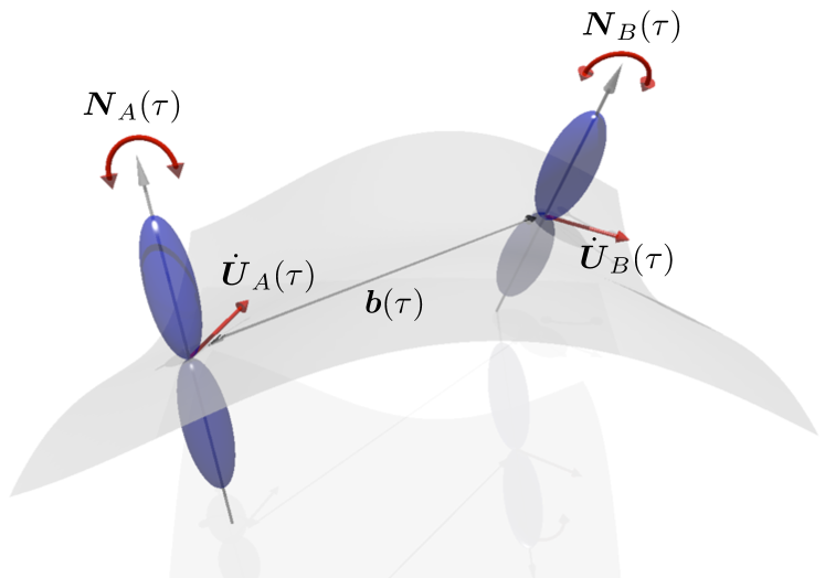
Figure 1: (color online). The sketch of a two-atom ($A$ and $B$) unit-cell basis of a dynamical graphene lattice. The $p_{z}$ orbitals (blue dumbells) instantaneously point along the directions $\bm{N}_{A,B}(\tau)$ normal to the graphene substrate (gray), which rotate at angular velocities $\dot{\bm{N}}_{A,B}(\tau)$. Here, $\bm{b}(\tau)$ is the instantaneous distance between the two atoms, and $\bm{\dot{U}}_{A(B)}(\tau)$ are their linear velocities.

The second mechanism affecting hopping strength involves only the out-of-plane displacement $h(\bm{r})$. As already mentioned, such distortions cause rotations of the atomic $p_{z}$ and the hybridized sp² orbitals, which become intermixed, thus modifying the tunneling Hamiltonian Castro Neto et al. (2009). To quantify the amount of orbital mixture, we introduce the normal to the surface and the unit vector connecting neighboring atoms at the position $\bm{R}_{s}$, respectively Kim and Neto (2008):

$$\bm{N}_{s}=\frac{\hat{\bm{z}}-\bm{\nabla}h(\bm{R}_{s})}{\sqrt{1+[\bm{\nabla}h(\bm{R}_{s})]^{2}}}\,,\,\,\,\bm{d}_{s,p}=\frac{\bm{b}_{p}+\hat{\bm{z}}\delta h_{p}(\bm{R}_{s})}{\sqrt{a^{2}+[\delta h_{p}(\bm{R}_{s})]^{2}}}\,,$$ (5)

where $\delta h_{p}(\bm{R}_{s})\equiv h(\bm{R}_{s}+\bm{b}_{p})-h(\bm{R}_{s})$. In the flat graphene, we can write Bardeen (1961) $t_{0}=\langle p_{z,A}|H-E_{0}|p_{z,B}\rangle\approx-2.8\,{\rm eV}$ and $t_{0}^{\prime}=\langle p_{y,A}|H-E_{0}|p_{y,B}\rangle\approx 8.4\,{\rm eV}$, where $\bm{R}_{B}=\bm{R}_{A}+\bm{b}_{3}$, $H$ is the full microscopic single-particle Hamiltonian in the lattice, and $E_{0}$ is the energy corresponding to the $p$ orbitals in an isolated carbon atom. In a curved graphene sheet, this is generalized to $t_{p}(\bm{R}_{s})=\langle\bm{N}_{s}\cdot\bm{p}_{s}|H-E_{0}|\bm{N}_{p}\cdot\bm{p}_{p}\rangle$, with $\bm{p}=(p_{x},p_{y},p_{z})$ being the $p$-orbital wave functions at a respective position in the lattice, $\bm{R}_{s}$ or $\bm{R}_{p}\equiv\bm{R}_{s}+\bm{b}_{p}$. We thus get for the change in tunneling due to curvature:

$$\delta t_{p}^{(\pi)}(\bm{R}_{s})=t_{0}(\bm{N}_{s}\cdot\bm{N}_{p}-1)+(t_{0}^{\prime}-t_{0})(\bm{N}_{s}\cdot\bm{d}_{s,p})(\bm{N}_{p}\cdot\bm{d}_{s,p})$$

$$\approx-\frac{t_{0}}{2}\left[(\bm{b}_{p}\cdot\bm{\nabla})\bm{\nabla}h(\bm{R}_{s})\right]^{2}-\frac{t_{0}^{\prime}-t_{0}}{4a^{2}}\left[(\bm{b}_{p}\cdot\bm{\nabla})^{2}h(\bm{R}_{s})\right]^{2}\,.$$ (6)

In this case too the changes in the tunneling $t_{p}$ lead to a fictitious gauge potential $A^{(\pi)}_{i}=2\sum_{p}\epsilon_{ij}b_{p}^{j}\delta t^{(\pi)}_{p}/3t_{0}a^{2}$. Written explicitly, the gauge field components $A^{(\pi)}_{i}(\bm{r})$ read:

$$A^{(\pi)}_{i}(\bm{r})=\frac{3}{8}\epsilon_{ij}\left(K_{jkl}\delta_{mn}+\frac{\mathfrak{t}}{3}K_{jkmln}\right)a\partial_{km}h(\bm{r})\partial_{ln}h(\bm{r})\,,$$ (7)

where $\mathfrak{t}\equiv(t_{0}^{\prime}-t_{0})/2t_{0}$ and the rank-5 tensor $K_{jkrsn}$ has the following nonzero elements: $K_{yyyyy}=-5$, $K_{yxxxx}=\dots=K_{xxxxy}=3$, and $K_{xxyyy}=K_{xyxyy}=\dots=K_{yyyxx}=1$. Expanding this out, say, for the $A^{(\pi)}_{x}$ component:

$$A^{(\pi)}_{x}= \frac{3(1+\mathfrak{t})}{8}a\left[(\partial^{2}_{x}h)^{2}-(\partial_{y}^{2}h)^{2}\right]$$

$$-\frac{\mathfrak{t}}{4}a\left[(\partial_{y}^{2}h)^{2}-(\partial^{2}_{x}h)(\partial^{2}_{y}h)-2(\partial_{xy}h)^{2}\right]\,.$$ (8)

We identify the first term, $\propto(1+\mathfrak{t})$, with the effective gauge field derived in Ref. Kim and Neto, 2008, while the second term, $\propto\mathfrak{t}$, is a new contribution that was previously overlooked in the literature (similarly, we obtain 2 terms for $A^{(\pi)}_{y}$) note1 .

One could try to extend the above static theory to the dynamical case by simply assuming the strain tensor $\hat{e}(\bm{r})$ and the height $h(\bm{r})$ to be time-dependent in the above expressions. The dynamic distortions then give rise to a fictitious electric field $\bm{E}(\tau)\equiv-\partial_{\tau}\bm{A}(\tau)$ ($\tau$ stands for real time), in addition to the aforementioned magnetic fields $\bm{B}=\bm{\nabla}\times\bm{A}$. The effect of such fictitious electric fields note3 have been studied recently in connection with both electron energy relaxation in carbon nanotubes von Oppen et al. (2009) and electron charge pumping in graphene Low et al. (2012). This quasistatic picture alone would, however, be incomplete, as it neglects Berry-phase effects engendered by the motion of the atomic basis orbitals themselves in the dynamically distorted lattice. To capture such effects in graphene, we start by deriving the effective electron tunneling Hamiltonian $H_{\rm eff}$ between two isolated $A/B$ sites in a time-dependent framework.

The full Hamiltonian of an electron in the potential $V(\bm{r},\tau)$ created by the two atoms, $A$ and $B$, is $H_{AB}(\tau)=p^{2}/2m+V(r,\tau)$, with $m$ being the bare electron mass. Typically, one then solves the Schrödinger equation approximatively by choosing a trial wave function $|\psi(\tau)\rangle=\left[c_{A}(\tau)|\psi_{A}\rangle+c_{B}(\tau)|\psi_{B}\rangle\right]\exp{(-iE_{0}\tau)}$, where $|\psi_{A,B}\rangle\equiv|\bm{N}_{A,B}\cdot\bm{p}_{A,B}\rangle$ and $c_{A,B}$ respectively stand for the atomic wave functions and their amplitudes at time $\tau$, and derive an effective Hamiltonian $H_{\rm eff}$ in the $A,B$ subspace. However, these single-atom basis wave functions are not instantaneous eigenstates of the two-atom Hamiltonian $H_{AB}$, which has nonzero matrix elements between the states $|\psi_{A,B}\rangle$ and the other orbitals outside this effective subspace. In the static situation, one can neglect such couplings, as their effect on $H_{\rm eff}$ appears in second order in perturbation theory with respect to the inverse atomic energy splittings, while, on the other hand, the direct coupling in the $|\psi_{A,B}\rangle$ subspace is first order and does not suffer from the energy mismatch. For the time-dependent case, in contrast, the intra-atomic electronic structure is itself perturbed by dynamics, which requires one to systematically account for the associated excursions outside of the effective subspace $|\psi_{A,B}\rangle$.

To capture such higher-order effects, we perform a more general time-dependent expansion: $|\psi^{\prime}(\tau)\rangle=|\psi(\tau)\rangle+\sum_{\alpha=A,B;n\notin\bm{p}_{\alpha}}c_{n,\alpha}(\tau)|n_{\alpha}\rangle\exp{(-iE_{n}\tau)}$, with $c_{n,\alpha}(\tau)$ , $|n_{\alpha}\rangle$, and $E_{n}$ being respectively the amplitude, wave function, and energy of electron in an excited orbital $n$. Substituting this expression into the Schrödinger equation, $i\partial_{\tau}|\psi^{\prime}(\tau)\rangle=H_{AB}|\psi^{\prime}(\tau)\rangle$, leads to the following set of differential equations for $c_{n,\alpha}(\tau)$:

$$i\dot{c}_{n,\alpha}(\tau)=\sum_{n^{\prime},\alpha^{\prime}}c_{n^{\prime},\alpha^{\prime}}(\tau)\langle n_{\alpha}|H_{AB}-E_{n}-i\partial_{\tau}|n^{\prime}_{\alpha^{\prime}}\rangle e^{i(E_{n}-E_{n^{\prime}})\tau}\,.$$ (9)

We will solve these equations only approximatively, in perturbation theory, assuming the time dependence of $H_{AB}$ is slow on the time scale $\tau_{d}\sim\Delta E$, with $\Delta E$ being the typical orbital level splitting, so that the system stays mostly in a state spanned by the $p$ orbitals. Then, taking $c_{n,\alpha}(\tau)\approx 0$ for excited orbitals, and $|c_{A}(\tau)|^{2}+|c_{B}(\tau)|^{2}\approx 1$, we obtain in leading order for $n\notin p_{\alpha}$:

$$c_{n,\alpha}(\tau) \simeq-\sum_{\alpha^{\prime}}c_{\alpha^{\prime}}(\tau)\frac{\langle n_{\alpha}|H_{AB}-E_{n}-i\partial_{\tau}|n_{\alpha^{\prime}}\rangle}{E_{n}-E_{0}}e^{i(E_{n}-E_{0})\tau}+F(\tau)\,,$$ (10)

where $F(\tau)$ is a function that varies slowly on the time scale $\tau_{d}$. By substituting this expression in the equations for $c_{A,B}(\tau)$ and neglecting all the fast oscillating terms $\propto\exp{[i(E_{0}-E_{n})\tau]}$, we end up with the effective Schrödinger equation $i\dot{\bm{c}}(\tau)=H_{\rm eff}\bm{c}(\tau)$, where $H_{\rm eff}\simeq t\,\Sigma_{x}+\delta\tilde{t}\,\Sigma_{y}$, with $\delta\tilde{t}=\delta\tilde{t}^{(G)}+\delta\tilde{t}^{(\pi)}$ and

$$\delta\tilde{t}^{(G)}(\tau)= mt(\tau)\dot{\bm{U}}(\tau)\cdot\bm{b}(\tau)\,,$$ (11)

$$\delta\tilde{t}^{(\pi)}(\tau)= \frac{1}{2}\left(\left\langle\bm{N}_{A}\cdot\bm{p}_{A}|\dot{\bm{N}}_{B}\cdot\bm{p}_{B}\right\rangle-\left\langle\dot{\bm{N}}_{A}\cdot\bm{p}_{A}|\bm{N}_{B}\cdot\bm{p}_{B}\right\rangle\right)\,.$$ (12)

Here, $\bm{U}(\tau)\equiv\bm{u}(\tau)+\hat{\bm{z}}h(\tau)$ is the sum of in-plane and out-of-plane displacements of the center-of-mass of the two atoms, $\bm{b}(\tau)$ is the distance vector connecting the two atoms, $t(\tau)\equiv t_{0}+\delta t(\tau)\approx\langle\psi_{A}|p^{2}/2m+V(\bm{r},\tau)-E_{0}|\psi_{B}\rangle$ is the quasistatic tunneling amplitude discussed above [i.e., $\delta t=\delta t^{(\beta)}+\delta t^{(\pi)}$], $\bm{c}(\tau)\equiv(c_{A}(\tau),c_{B}(\tau))$, and $\bm{\Sigma}$ are Pauli matrices that act in this $A,B$ basis. Equation (11) can be recognized as a local Galilean boost, for the derivation of which it is crucial to take into account corrections stemming from higher-orbital excursions, Eq. (10) note2 . Eq. (12) is due to rotations of the local atomic $p$ orbitals (see Fig. 1): It emerges in the time-dependent picture as a Berry-phase correction to the tunneling term defined in Eq. (6). Note that the Galilean boost term can be re-exponentiated to give $t\rightarrow t^{\prime}=t\exp{\left(-im\dot{\bm{U}}\cdot\bm{b}\right)}$, as is expected according to the Peierls substitution in the moving frame of reference.

We are now equipped to construct the full graphene Hamiltonian in the dynamical case. The new (dynamic) corrections to the tunneling, $\delta\tilde{t}^{(G,\pi)}$, are purely imaginary, while the quasistatic ones, $\delta t^{(\beta,\pi)}$, are purely real, which allows us to write $t_{\rm tot}=t_{0}+\delta t+i\delta\tilde{t}$, with $\delta t=\delta t^{(\beta)}+\delta t^{(\pi)}$ and $\delta\tilde{t}=\delta\tilde{t}^{(G)}+\delta\tilde{t}^{(\pi)}$. The resultant effective Hamiltonian around the $K$ point still has the form of Eq (2), but with the total gauge field $\bm{A}_{\rm tot}(\bm{r},\tau)\equiv\bm{A}(\bm{r},\tau)+\bm{\tilde{A}}(\bm{r},\tau)$ being the sum of the quasistatic and dynamic contributions, respectively, where $A_{i}=2\sum_{p}\epsilon_{ij}b_{p}^{j}\delta t_{p}/3t_{0}a^{2}$ was evaluated already and $\tilde{A}_{i}=2\sum_{p}b_{p}^{i}\delta\tilde{t}_{p}/3t_{0}a^{2}$ consists of:

$$\tilde{A}^{(G)}_{i}\simeq -ma\left[\dot{u}_{i}+a\dot{h}\,\partial_{i}h+\frac{a^{2}}{2}K_{ijk}\dot{h}\,\partial_{jk}h\right]\,,$$ (13)

$$\tilde{A}^{(\pi)}_{i}\simeq -\frac{1}{t_{0}}\left[s_{0}\delta_{ij}\delta_{kl}+\frac{s^{\prime}_{0}-s_{0}}{8}K_{ijkl}\right]\partial_{l}\dot{h}\,\partial_{jk}h$$

$$+\frac{a}{2t_{0}}\left[s_{0}K_{ijk}\delta_{lm}+\frac{s^{\prime}_{0}-s_{0}}{8}K_{ijlkm}\right]\partial_{km}\dot{h}\,\partial_{jl}h\,,$$ (14)

where $K_{ijsr}=\delta_{ij}\delta_{kl}+\delta_{ik}\delta_{jl}+{\delta_{il}\delta_{jk}}$, $s_{0}=\langle p_{z,A}|p_{z,B}\rangle$ and $s_{0}^{\prime}=\langle p_{y,A}|p_{y,B}\rangle$ (taking their values to be at 0.1 and -0.3, respectively) are orbital overlaps between the nearest-neighbor atoms for $\bm{R}_{B}=\bm{R}_{A}+\bm{b}_{3}$. We find that in the presence of both in-plane and out-of-plane time-dependent distortions, the effective Hamiltonian for graphene is complemented by the new, purely dynamic, gauge fields $\bm{\tilde{A}}^{(G)}$ and $\bm{\tilde{A}}^{(\pi)}$, which form the main result of our paper. The leading-order terms $\propto h(\bm{r},\tau)$ in $\bm{\tilde{A}}^{(G,\pi)}$ appear formally as the dynamic analogue of the static $\bm{A}^{(\beta,\pi)}$ terms, respectively, by substituting one partial spatial derivative $\partial_{i}h\rightarrow\partial_{\tau}h$, with $i=x,y$, in the static fields. The next-order terms are proportional to the (time) derivative of curvature, $\propto\partial_{ij}\dot{h}$, which do not appear in our static expansion. Repeating the analysis for the $K^{\prime}$ point (either microscopically or by time reversal of the $K$-point solution) shows that we need to substitute $\bm{A}\rightarrow-\bm{A}$, while $\bm{\tilde{A}}$ has the same sign and magnitude as at the $K$ point. This has profound implications on the electron dynamics, as the gauge fields acting at the $K$ and $K^{\prime}$ valleys are no longer equal in magnitude, and this asymmetry can lead to time-reversal-breaking observable electromagnetic properties, like charge currents and (quantum) Hall effect.

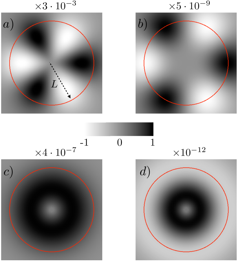
Figure 2: The radial projection of the fictitious gauge field, $A_{r}(\bm{r})\equiv\bm{A}(\bm{r})\cdot\hat{\bm{r}}$, stemming from different mechanisms discussed in the main text, for a Gaussian bump of radius $L=100$ nm, height $h_{0}=10$ nm and $\omega=10^{9}$ s^-1. From left to right: a) static strain-dependent component $A_{r}^{(\beta)}$, b) static curvature-dependent component $A_{r}^{(\pi)}$, c) dynamic Galilean component $\tilde{A}_{r}^{(G)}$, d) dynamic curvature-dependent component $\tilde{A}_{r}^{(\pi)}$. All the gauge fields are expressed in units of $a^{-1}$, where $a=1.42$ Å.

As a particular example, we assume a time-dependent gaussian bump, $h(\bm{r},\tau)=h_{0}\exp{(-r^{2}/L^{2})}\cos{(\omega\,\tau)}$, with $h_{0}$ and $L$ being the amplitude and the extension of the bump, respectively. In Fig. 2, we plot the resultant gauge field component $A_{x}$ for the four different mechanisms: strain, Eq. (4), static curvature, Eq. (7), Galilean boost, Eq. (13), and dynamic curvature, Eq. (14). We see that for a given Dirac point ($K$ point in Fig. 2), the static gauge fields $A_{r}^{(\beta,\pi)}(\bm{r})$ are invariant under $C_{3}$ rotations, and under $C_{6}$ rotations complemented by overall sign change (which corresponds to time reversal), while the dynamic terms $\tilde{A}_{r}^{(G,\pi)}$ are simply invariant under $C_{6}$ rotations. Let us now consider the quantitative difference between the four different gauge fields (restoring $\hbar$):

$$|\bm{A}^{(\beta)}|\propto\frac{\beta h^{2}_{\rm 0}}{aL^{2}} =\frac{\beta}{a}\left(\frac{h_{\rm 0}}{L}\right)^{2}\,,\,\,\,|\bm{A}^{(\pi)}|\propto\frac{ah^{2}_{\rm 0}}{L^{4}}=\frac{1}{a}\left(\frac{a}{L}\right)^{2}\left(\frac{h_{\rm 0}}{L}\right)^{2},$$

$$|\bm{\tilde{A}}^{(G)}| \propto\frac{m\omega h^{2}_{\rm 0}}{\hbar L}=\frac{1}{a}\frac{\hbar\omega}{E_{L}}\frac{a}{L}\left(\frac{h_{\rm 0}}{L}\right)^{2}\,,$$ (15)

$$|\bm{\tilde{A}}^{(\pi)}| \propto\frac{\hbar\omega h_{0}^{2}}{|t_{0}|L^{3}}=\frac{1}{a}\frac{\hbar\omega}{|t_{0}|}\frac{a}{L}\left(\frac{h_{\rm 0}}{L}\right)^{2},$$

where $E_{L}=\hbar^{2}/mL^{2}$ is the free-electron energy with a wave number corresponding to the distortion size $L$. While it may appear that the largest contribution is that arising from strain ($\propto\beta$), it is in fact overestimated here, since graphene is elastically extremely stiff for strain deformations Lee et al. (2008); Poot and van der Zant (2008); Frank et al. (2007); Bunch et al. (2007); Chen et al. (2009). Bending, on the other hand, costs much less energy Castro Neto et al. (2009), so that the low-energy height perturbations should favor profiles with minimal strain Rainis et al. (2011). While we treat the planar distortions [setting them to zero in Eq. (15)] and the height profile $h(\bm{r},\tau)$ as independent parameters, in practice, a self-consistent treatment of elastic properties would be necessary, by balancing bending, shear, and compression energies Kim and Neto (2008). While addressing this problem in detail is important in view of quantifying the strength of the emergent gauge fields, such a calculation is beyond our immediate goals and will be presented elsewhere Pramey2012 . It suffices to say that, due to different spatiotemporal scaling (once the strain and bending are relaxed for a given height profile), we can easily envision geometric and dynamic limits where different terms in Eq. (15) would provide the dominant contribution.

This work was supported by the NSF under Grant No. DMR-0840965. Fruitful discussions with Antonio H. Castro Neto are gratefully acknowledged.

References

- Novoselov et al. (2004) K. S. Novoselov, A. K. Geim, S. V. Morozov, D. Jiang, Y. Zhang, S. V. Dubonos, I. V. Grigorieva, and A. A. Firsov, Science, 306, 666 (2004).
- Novoselov et al. (2005) K. S. Novoselov, A. K. Geim, S. V. Morozov, D. Jiang, M. I. Katsnelson, I. V. Grigorieva, S. V. Dubonos, and A. A. Firsov, Nature, 438, 197 (2005).
- Zhang et al. (2005) Y. Zhang, Y.-W. Tan, H. L. Stormer, and P. Kim, Nature, 438, 201 (2005).
- Geim and Novoselov (2007) A. K. Geim and K. S. Novoselov, Nat Mater, 6 (2007).
- Castro Neto et al. (2009) A. H. Castro Neto, F. Guinea, N. M. R. Peres, K. S. Novoselov, and A. K. Geim, Rev. Mod. Phys., 81, 109 (2009).
- Kotov et al. (2012) V. N. Kotov, B. Uchoa, V. M. Pereira, F. Guinea, and A. H. Castro Neto, Rev. Mod. Phys., 84, 1067 (2012).
- Sundaram and Niu (1999) G. Sundaram and Q. Niu, Phys. Rev. B, 59, 14915 (1999).
- Wallace (1947) P. R. Wallace, Phys. Rev., 71, 622 (1947).
- Vozmediano et al. (2010) M. Vozmediano, M. Katsnelson, and F. Guinea, Phys. Rep., 496, 109 (2010).
- Lee et al. (2008) C. Lee, X. Wei, J. W. Kysar, and J. Hone, Science, 321, 385 (2008).
- Poot and van der Zant (2008) M. Poot and H. S. J. van der Zant, Applied Physics Letters, 92, 063111 (2008).
- Frank et al. (2007) I. W. Frank, D. M. Tanenbaum, A. M. van der Zande, and P. L. McEuen (AVS, 2007) pp. 2558–2561.
- Bunch et al. (2007) J. S. Bunch, A. M. van der Zande, S. S. Verbridge, I. W. Frank, D. M. Tanenbaum, J. M. Parpia, H. G. Craighead, and P. L. McEuen, Science, 315, 490 (2007).
- Chen et al. (2009) C. Chen, S. Rosenblatt, K. I. Bolotin, W. Kalb, P. Kim, I. Kymissis, H. L. Stormer, T. F. Heinz, and J. Hone, Nature Nanotech, 4, 861 (2009).
- Pereira and Castro Neto (2009) V. M. Pereira and A. H. Castro Neto, Phys. Rev. Lett., 103, 046801 (2009).
- Guinea et al. (2010) F. Guinea, M. I. Katsnelson, and A. K. Geim, Nature Phys, 6, 30 (2010).
- Medvedyeva and Blanter (2011) M. V. Medvedyeva and Y. M. Blanter, Phys. Rev. B, 83, 045426 (2011).
- Kim et al. (2011) K.-J. Kim, Y. M. Blanter, and K.-H. Ahn, Phys. Rev. B, 84, 081401 (2011).
- Katsnelson et al. (2006) M. I. Katsnelson, K. S. Novoselov, and A. K. Geim, Nature Phys, 2, 620 (2006).
- Itzykson and Zuber (2006) C. Itzykson and J.-B. Zuber, Quantum Field Theory (Dover, New York, 2006).
- Kim and Neto (2008) E.-A. Kim and A. H. C. Neto, Europhys. Lett., 84, 57007 (2008).
- Bardeen (1961) J. Bardeen, Phys. Rev. Lett., 6, 57 (1961).
- (23) We note that Eq. (8) reduces to the expression found in Ref. Kim and Neto, 2008 when, for example, . Geometrically, this means the rotated orbitals are lying in the same plane, which simplifies expression for Kim and Neto (2008). This does not hold for a general noncoplanar case, however, and one needs to use the full expression, Eq. (6), to obtain the correct gauge field .
- (24) We note that there is also a contribution to the electric field due to modulation of the deformation potential in the distorted lattice, which is given by Suzuura and Ando (2002). However, we disregard these terms here, as they do not give rise to any electromotive forces either over closed circuits or segments of graphene with unstrained boundaries.
- Suzuura and Ando (2002) H. Suzuura and T. Ando, Phys. Rev. B 65, 235412 (2002).
- von Oppen et al. (2009) F. von Oppen, F. Guinea, and E. Mariani, Phys. Rev. B, 80, 075420 (2009).
- Low et al. (2012) T. Low, Y. Jiang, M. Katsnelson, and F. Guinea, Nano Letters, 12, 850 (2012).
- (28) In fact, the result in Eq. (11) is entirely due to transitions outside the effective subspace , via cross terms involving the Hamiltonian and the operator. The contributions arising from the direct transitions within the subspace are exactly cancelled, in a nontrivial way, by a subset of the aforementioned cross terms.
- Rainis et al. (2011) D. Rainis, F. Taddei, M. Polini, G. León, F. Guinea, and V. I. Fal’ko, Phys. Rev. B, 83, 165403 (2011).
- (30) P. Upadhyaya et al. (unplublished).