Abstract

In this thesis I explore challenging discrete energy minimization problems that arise mainly in the context of computer vision tasks. This work motivates the use of such “hard-to-optimize” non-submodular functionals, and proposes methods and algorithms to cope with the NP-hardness of their optimization. Consequently, this thesis revolves around two axes: applications and approximations. The applications axis motivates the use of such “hard-to-optimize” energies by introducing new tasks. As the energies become less constrained and structured one gains more expressive power for the objective function achieving more accurate models. Results show how challenging, hard-to-optimize, energies are more adequate for certain computer vision applications. To overcome the resulting challenging optimization tasks the second axis of this thesis proposes approximation algorithms to cope with the NP-hardness of the optimization. Experiments show that these new methods yield good results for representative challenging problems.

See pages 3,2 of ./abstract_heb.pdf

Part I Introduction

In this thesis I explore challenging discrete energy minimization problems that arise mainly in the context of computer vision. From binary energies for figure-ground segmentations through multi-label semantic segmentation, stereo, denoising, to inpainting and image editing (e.g., Szeliski et al. (2008); Pritch et al. (2009); Bagon (2012)). These energies usually involve thousands of variables and dozens of discrete states. Moreover, most of the energies in this domain are pair-wise energies, that is, they only involve interactions between pairs of neighboring variables.

The optimization of these discrete energies is known to be NP-hard in most cases (Boykov et al. (2001)). Still, despite this theoretical hardness, instances of these energies that have special properties may give rise to polynomial time global optimal algorithms. Other instances with slightly different properties allow, in practice, for good and efficient approximation schemes.

The next chapter (Chap. 1) reviews previous work related to discrete pair-wise energy functions and their optimization. It outlines the properties and conditions under which global optimization is feasible, and the conditions required for successful practical approximations. Chapter 1 also surveys several key approximation algorithms. It provides a brief outline of the properties of the energy that must be met in order for each algorithm to succeed. The conclusion of this survey is that discrete pair-wise energies may be broadly classify into two categories: ⁢

smoothness-encouraging energies: energies that favor configurations with neighboring variables taking the same discrete state.⁢

contrast-enhancing energies: energies that encourage solutions where neighboring variables take different states.⁢

So far the energies mainly used in computer vision tasks are of the first category: smoothness-encouraging (see e.g., Szeliski et al. (2008)). These smoothness-encouraging energies allow for efficient approximation schemes. On the other hand, contrast-enhancing energies are far more challenging when it comes to optimization, and are indeed less popular in practice.

In this thesis I would like to step outside of this “comfort-zone” of the smoothness-encouraging energies and explore more challenging discrete energies. This work revolves around two axes:

1. Applications: The first motivates the use of such “hard-to-optimize” functionals by introducing new applications. As the energies become less constrained and structured one gains more expressive power for the objective function achieving more accurate models. Results show how contrast-enhancing, hard-to-optimize, functionals are more adequate for certain computer vision tasks.

2. Approximations: To overcome the resulting challenging optimization tasks the second axis of this thesis proposes methods and algorithms to cope with the NP-hardness of this optimization. Experiments show that these new methods yield good results for representative challenging problems.

Chapter 1 Discrete Pair-wise Energies – a Review

Discrete energy minimization is a ubiquitous task in computer vision. From binary energies for figure-ground segmentations through multi-label semantic segmentation, stereo, denoising, to inpainting and image editing (e.g., Szeliski et al. (2008); Pritch et al. (2009); Bagon (2012)). In my thesis I focus on various types of minimization problems of pair-wise energies as they arise in different computer vision applications. These discrete optimization problems are, in general, NP-hard. Yet, there are cases in which the minimization of a pair-wise energy can be solved exactly in polynomial time. In this introductory chapter I survey different properties of discrete pair-wise energies. I show how these properties of the energies relate to the inherent difficulty of the optimization task. Some properties entail exact optimization algorithms, while other properties admit efficient approximations. The most important property is “smoothness-encouraging”: an energy that prefers the labels of neighboring variables to be the same. For these “smoothness-encouraging” energies there exist efficient approximate minimization algorithms. In contrast, energies that encourage neighboring variables to have different labels are much more challenging to minimize. For these “contrast-enhancing” energies existing algorithms provide poor approximations. This thesis focuses on the optimization of these challenging “contrast-enhancing” energies.

1 Pair-wise Energy Function

Before diving into the minimization task, this section presents the discrete pair-wise energy function and the notations that are used in this thesis. It also provides some insights and motivation for the use of such energies.

A discrete pair-wise energy is a functional of the form

$$F\left(\mathbf{x}\right)=\sum_{ij\in\mbox{$\mathcal{E}$}}\varphi_{ij}\left(x_{i},x_{j}\right)+\sum_{i}\varphi_{i}\left(x_{i}\right)$$ (1)

It is defined over $n$ variables ($x_{i}$, $i=1,\ldots,n$), each taking one of $l$ discrete labels ($x_{i}\in\left\{1,\ldots,l\right\}$), where $\mathcal{E}$ represents a set of neighboring variables. The term $\varphi_{i}\left(x_{i}\right)$ is a unary term reflecting the compatibility of label $x_{i}$ to variable $i$ (also known as a “data term”). The pair-wise term, $\varphi_{ij}\left(x_{i},x_{j}\right)$ reflects the interaction between labels $x_{i}$ and $x_{j}$ assigned to variables $i$ and $j$ respectively.

If we were to discard the pair-wise term, minimizing energy (1) is simply choosing the label that best fit each variable separately. However, the presence of the pair-wise term introduces dependencies between the different variables and turns the optimization into a much more complicated process. Despite the local nature of the pair-wise term – binding the values of only neighboring variables introduces global effects on the overall optimization. Propagating the information from the local pair-wise terms to form a global solution is a major challenge for the optimization of Eq. (1).

The energy function of Eq. (1) has an underlying structure defined by the choice of interacting neighbors. It is common to associate with $F\left(\mathbf{x}\right)$ a graph $\mbox{$\mathcal{G}$}=\left(\mbox{$\mathcal{V}$},\mbox{$\mathcal{E}$}\right)$, where the set of nodes $\mbox{$\mathcal{V}$}=\left\{1,\ldots,n\right\}$ represents the variables, and the edges $\mathcal{E}$ represents the interacting neighboring pairs.

The following example shows how such discrete functional may arise in a well studied computer vision application. This example also illustrates the relation between discrete optimization and inference in graphical models.

Example 1.1.

Example: Stereo reconstruction via MRF representation

Given a rectified stereo pair of images, the goal is to find the disparity of each pixel in the reference image. The true disparity of each pixel is a random variable denoted by $x_{i}$ for the pixel at location $i$. Each variable can take one of $L$ discrete states, which represent the possible disparities at that point. For each possible disparity value, there is a cost associated with matching the pixel in the reference image to the corresponding pixel in the other image at that disparity value. Typically, this cost is based on the intensity differences between the two pixels, $y_{i}$, which is an observed quantity. We denote this cost by $\Phi(x_{i},y_{i})$. It relates how compatible a disparity value $x_{i}$ is with the observed intensity difference $y_{i}$. A second function $\Psi(x_{i},x_{j})$ expresses the disparity compatibility between neighboring pixels. This function usually expresses the prior assumption that the disparity field should be smooth. Examples of such prior that are commonly used are the Potts model:

$$\Psi(x_{i},x_{j})=\left\{\begin{array}[]{cl}1&\mbox{if $x_{i}=x_{j}$}\\ 0&\mbox{otherwise}\end{array}\right.$$ (2)

the $\ell_{1}$ similarity:

$$\Psi(x_{i},x_{j})\propto e^{-\left|x_{i}-x_{j}\right|}$$ (3)

or its robust (truncated) version:

$$\Psi(x_{i},x_{j})\propto e^{-\min\left\{\left|x_{i}-x_{j}\right|,\tau\right\}}$$ (4)

With the two functions $\Phi$ and $\Psi$ the joint probability for an assignment of disparities to pixels can be written as:

$$P(\mathbf{x},\mathbf{y})\propto\prod_{ij\in\mbox{$\mathcal{E}$}}\Psi(x_{i},x_{j})\prod_{i}\Phi(x_{i},y_{i})$$ (5)

where $\mathbf{x}$ is an assignment of a disparity value for each pixel $i$. $x_{i}$ is the hidden variable (disparity) at location $i$ and $y_{i}$ is the observed variable (intensity difference) at location $i$. ${ij\in\mbox{$\mathcal{E}$}}$ represent a pair of neighboring nodes and is usually taken as a regular 4-connected grid over the image domain.

The resulting graphical model is known as a pairwise Markov Random Field. Although the compatibility functions only consider adjacent variables, each variable is still able to influence every other variable in the field via these pairwise connections.

We look for a disparity assignment such that the labeling $\mathbf{x}^{\star}$ maximizes the joint probability, i.e.,

$$\mathbf{x}^{\star}=\underset{\mathbf{x}}{\operatorname{argmax}}\leavevmode\nobreak\ \leavevmode\nobreak\ \leavevmode\nobreak\ P(\mathbf{x},\mathbf{y})$$ (6)

Assuming uniform prior over all configurations $\mathbf{x}$, the Maximum A Posteriori (MAP) estimator is equivalent to

$$\mathbf{x}^{\star}=\underset{\mathbf{x}}{\operatorname{argmax}}\leavevmode\nobreak\ \leavevmode\nobreak\ \leavevmode\nobreak\ P(\mathbf{x}|\mathbf{y})$$ (7)

Maximizing the posterior probability is equivalent to minimizing an energy functional of the form (1). Taking $-\log$ of (5) yields the following function

$$F\left(\mathbf{x}\right)=\sum_{ij\in\mbox{$\mathcal{E}$}}-\log\Psi(x_{i},x_{j})+\sum_{i}-\log\Phi(x_{i},y_{i})$$ (8)

This equation can be expressed as

$$\sum_{ij\in\mbox{$\mathcal{E}$}}\varphi_{ij}\left(x_{i},x_{j}\right)+\sum_{i}\varphi_{i}\left(x_{i}\right)$$ (9)

where $\varphi_{ij}\left(x_{i},x_{j}\right)\triangleq-\log\Psi(x_{i},x_{j})$ and $\varphi_{i}\left(x_{i}\right)\triangleq-\log\Phi(x_{i},y_{i})$.

Thus MAP (maximum a-posteriori) inference in graphical models such as MRF and conditional random fields (CRF) boils down to the optimization of a discrete pair-wise energy functional of the form Eq. (1) which is the focus of this thesis.

Energy functions of the form Eq. (1) arise in many graphical models (MRFs and CRFs) (see e.g., Blake et al. (2011) and references therein). However, it is not restricted to that domain and are also encountered in a variety of other domains such as structural learning (e.g., Nowozin and Lampert (2011)), and as the inference part of discriminative models (e.g., structural SVM Taskar et al. (2003); Tsochantaridis et al. (2006)). This thesis explores some challenging instances of these energies and explores new methods for improved minimization approaches for these hard-to-optimize energies.

2 Minimization of Discrete Pair-wise Energies

The energy function of Eq. (1) presented in the previous section is used in many applications to evaluate how compatible is a certain discrete solution $\mathbf{x}$ to a given problem. It is now desired to find the best solution for the given problem by finding a solution $\mathbf{x}^{\star}$ with the lowest energy. That is, solving the optimization problem

$$\mathbf{x}^{\star}=\arg\min_{\mathbf{x}}F\left(\mathbf{x}\right)$$ (10)

over all discrete solutions $\mathbf{x}$.

In general, the optimization problem (10) is NP-hard. Known hard combinatorial problems such as max-cut, multi-way cut and many others may be formulated in the form of (10) (see e.g., Boykov et al. (2001)). Yet, there are special instances of problem (10) which can be optimized exactly in polynomial time. The main two factors that affect the difficulty of the optimization problem (10) are:

1. The underlying graph structure, $\mathcal{E}$.

2. Mathematical properties of the pair-wise interactions, $\varphi_{ij}$.

When the underlying graph $\mathcal{E}$ has no cycles (that is, $\mathcal{E}$ has a tree structure) optimization of (10) is fairly straight-forward: By propagating information back and forth from the leafs to the root convergence to global minimum is attained. This information propagation is often referred to as belief-propagation (BP) (Pearl (1988); Koller and Friedman (2009)). A cycle-free graph is crucial for this rapid polynomial time convergence of this message-passing scheme: Every path from root to leaf is unique and therefore consensus along path is attained in a single forward backward pass. However, when $\mathcal{E}$ has cycles, paths between the different variables are no longer unique and may give rise to contradicting messages. These contradictions introduce an inherent difficulty to the optimization process making it NP-hard in general.

Despite the inherent difficulty of optimizing (10) over a cyclic graph $\mathcal{E}$, there are instances of problem (10) that can still be efficiently minimized when the pair-wise terms, $\varphi_{ij}$, meet certain conditions. The next few sections explore these conditions in more detail, providing pointers to existing optimization methods that succeed in exploiting special structures of $\varphi_{ij}$ to suggest methods and guarantees on the optimization process. For simplicity, we start in Sec. 3 with the special case of discrete binary variables, that is $\mathbf{x}\in\left\{0,1\right\}^{n}$. Then we move on, in Sec. 4, to the multilabel case of discrete variables taking one of multiple possible states, $\mathbf{x}\in\left\{1,\ldots,l\right\}^{n}$.

3 Binary problems

Binary optimization problems are of the form (10) where the solution space is restricted to binary vectors only, i.e., $\mathbf{x}\in\left\{0,1\right\}^{n}$.

The most basic property of binary functionals is submodularity. This property is defined as follows:

Definition 3.2 (Binary submodular).

A pair-wise function $F\left(\mathbf{x}\right)$ defined for binary vectors $\mathbf{x}$ is submodular iff $\forall i,j\in\mbox{$\mathcal{E}$}$: $\varphi_{ij}\left(0,0\right)+\varphi_{ij}\left(1,1\right)\leq\varphi_{ij}\left(1,0\right)+\varphi_{ij}\left(0,1\right)$

Close inspection of Def. 3.2 reveals that a submodular function assigns lower energy to smooth configurations (i.e. to $x_{i}=x_{j}$) than to “contrastive” configurations (i.e., to $x_{i}\neq x_{j}$). That is the “smooth” state $\varphi_{ij}\left(0,0\right)+\varphi_{ij}\left(1,1\right)$ has lower energy than the “contrastive” state $\left(1,0\right)+\varphi_{ij}\left(0,1\right)$. Fig. 1 provides an illustration of the space of all pair-wise energies.

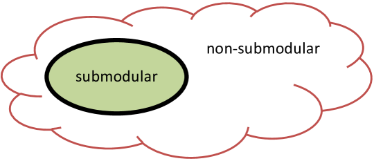
Figure 1: types of binary $F\left(\mathbf{x}\right)$: submodular vs. non-submodular. Green color indicates energies for which exact minimization can be done in polynomial time.

Submodularity is an important property of $\varphi_{ij}$ since exact optimization of binary submodular functions can be done in polynomial time regardless of the graph structure $\mathcal{E}$ (Greig et al. (1989)). One such optimization algorithm identifies a $1:1$ mapping between binary assignments $\mathbf{x}$ and cuts on a specially constructed graph. Careful choice of weights for the edges on this special graph gives rise to a $1:1$ mapping between the weight of a cut and $F\left(\mathbf{x}\right)$ of the appropriate binary assignment $\mathbf{x}$. This construction and choice of weights is illustrated in Fig. 3. The appropriate correspondences between assignments and graph-cuts, and between cut weight and energy are illustrated in Fig. 3. Once this $1:1$ mapping is established, optimizing $F\left(\mathbf{x}\right)$ is simply finding a minimum cut of the constructed graph. This can be done in polynomial time provided that all the weights of the edges are non-negative (Cormen et al. (2001)). Examining the details of this construction reveals that edge weights are non-negative iff the function $F\left(\mathbf{x}\right)$ is submodular. Details of this construction can be found in e.g., Greig et al. (1989); Boykov et al. (2001) and in more detail in Kolmogorov and Zabih (2004).

	$F\left(\mathbf{x}\right)=\varphi_{i}\left(x_{i}\right)+\varphi_{j}\left(x_{j}\right)+\varphi_{ij}\left(x_{i},x_{j}\right)$
	$\varphi_{i}$ $x_{i}=0$ $a$ $x_{1}=1$ $b$	$\varphi_{j}$ $x_{j}=0$ $c$ $x_{j}=1$ $d$	$\varphi_{ij}$ $x_{i}=0$ $x_{i}=1$ $x_{j}=0$ $e$ $f$ $x_{j}=1$ $g$ $h$
	Binary energy over two variables $i$ and $j$ parameterized by 8 parameters $a-h$.

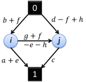
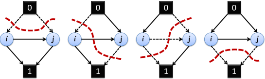
Figure 2: Graph construction: For a binary energy $F\left(\mathbf{x}\right)$ a weighted graph is constructed in the following way: Each variable $x_{i}$ has a corresponding node $i$. In addition, two special nodes (denoted in this figure as $0$ and $1$) are added. Two edges connect each $i^{th}$ node to the special nodes $0$ and $1$. In addition, an edge $(i,j)$ is added for each interacting pair of variables (for which $\varphi_{ij}$ exists). The weights of the edges are defined according to the parameters of the energy as illustrated in the figure. Note that the weight of the $(i,j)$ edge, $g+f-e-h$, is exactly $\varphi_{ij}(0,1)+\varphi_{ij}(1,0)-\varphi_{ij}(0,0)-\varphi_{ij}(1,1)$, this weight is non-negative iff $\varphi_{ij}$ is submodular.

cut	$\left\{0\right\}$, $\left\{1,i,j\right\}$	$\left\{0,j\right\}$, $\left\{1,i\right\}$	$\left\{0,i\right\}$, $\left\{1,j\right\}$	$\left\{0,i,j\right\}$, $\left\{1\right\}$
assignment $\mathbf{x}$	$x_{i}=1$, $x_{j}=1$	$x_{i}=1$, $x_{j}=0$	$x_{i}=0$, $x_{j}=1$	$x_{i}=0$, $x_{j}=0$
cut	$(b+f)$	$(b+f)$	$(a+e)+(d-f+h)$	$(a+e)$
weight	$+(d-f+h)$	$+c$	$+(g+f-e-h)$	$+c$
energy $F\left(\mathbf{x}\right)$	$b+d+h$	$b+f+c$	$a+g+d$	$a+e+c$

Figure 3: Binary energies and graph-cuts: All four possible cuts of the graph constructed in Fig. 3. A cut (dashed red) separates the two special nodes, $0$ from $1$. Cut edges (edges pointing from the $0$ side to the $1$ side) are marked with dash lines. First two rows show the $1:1$ mapping between a cut and an assignment to $\mathbf{x}$. Last two rows show the $1:1$ mapping between the weight of the cut (using the weights defined in Fig. 3) and the energy $F\left(\mathbf{x}\right)$ of the appropriate assignment.

However, when $F\left(\mathbf{x}\right)$ is not submodular (i.e., there exists at least one pair-wise term $\varphi_{ij}$ for which the submodularity inequality (3.2) does not hold) the optimization of $F\left(\mathbf{x}\right)$ becomes NP-hard (Rother et al. (2007)). In that case exact minimum cannot be guaranteed in polynomial time and an approximation is sought. One notable approach for approximating non-submodular binary optimization problems is by an extension of the min-cut approach. This method, called QPBO (Quadratic Pseudo-Boolean Optimization) was proposed by Hammer et al. (1984) and later extended by Rother et al. (2007). The main idea behind this approximation scheme is that when the energy function $F\left(\mathbf{x}\right)$ is non-submodular, the derived graph has edges with negative weights. Therefore, they propose to construct a redundant graph in which each variable is represented by two nodes (rather than only one as in the original construction). One node represents the case where the variable is assigned $0$ and the other node represents the case of assigning $1$ to the variable. This redundant representation eliminates the need for negative edge weights and thus a min-cut of the new graph can be computed in polynomial time. Looking at the resulting min-cut we can discern two cases for each variable: The first, in which the cut separates the two complementary nodes representing this variable. In this case, the cut clearly defines an optimal state for the variable (either $0$ or $1$). However, there is a second case in which both complementary nodes fall in the same side of the cut. In this case, we are unable to determine what is the proper assignment for this variable and the variable remains unlabeled.

Therefore, we can conclude that QPBO extends the min-cut approach to handle non-submodular binary energies. Recovery of the global minimum is no longer guaranteed, but the algorithm may recover a partial labeling that is guaranteed to be part of some globally optimal solution. However, in the extreme case it may happen that QPBO is unable to label any variable.

Table 1 summarizes the different types of pair-wise binary energy functions and the difficulty they entail on their optimization.

	Tree	Cyclic
submodular	Easy: mincut, BP	Easy: mincut
non-submodular	Easy: QPBO, BP	Hard

Table 1: Hardness of binary optimization: the computational “hardness” of a discrete minimization as a function of the underlying graph structure ($\mathcal{E}$), and the class of pair-wise interactions ($\varphi_{ij}$).

4 Multilabel problems

A multilabel discrete problem is the optimization of a discrete function $F\left(\mathbf{x}\right)$ of the form (1) defined over a finite discrete vector $\mathbf{x}\in\left\{1,\ldots,L\right\}^{n}$. As was shown in the previous section, properties of the pair-wise terms $\varphi_{ij}$ of $F\left(\mathbf{x}\right)$ have a crucial effect on the computational complexity of the optimization problem. For the binary case the only distinctive property was the submodularity of $F\left(\mathbf{x}\right)$. However, when discrete variables over more than two states are considered, there are more subtle types of pair-wise interactions that affect the ability to optimize, or at least efficiently approximate it. This section describes these various types of $\varphi_{ij}$ and their effect on the discrete optimization task.

The following definition of multilabel submodularity is given in Schlesinger and Flach (2006).

Definition 4.3 (Multilabel submodular).

Assume the labels ($\alpha,\beta,\ldots$) are fully ordered. Then $F\left(\mathbf{x}\right)$ is multilabel submodular iff $\forall i,j\in\mbox{$\mathcal{E}$}$ and $\forall\alpha\leq\gamma,\beta\leq\delta$ the following inequality holds

$$\varphi_{ij}\left(\alpha,\beta\right)+\varphi_{ij}\left(\gamma,\delta\right)\leq\varphi_{ij}\left(\alpha,\delta\right)+\varphi_{ij}\left(\gamma,\beta\right)$$ (11)

A slightly simpler and equivalent condition for submodularity uses the following condition:

$$\varphi_{ij}\left(\alpha,\beta\right)+\varphi_{ij}\left(\alpha+1,\beta+1\right)\leq\varphi_{ij}\left(\alpha,\beta+1\right)+\varphi_{ij}\left(\alpha+1,\beta\right)$$ (12)

$F\left(\mathbf{x}\right)$ is multilabel submodular iff (12) holds for all labels $\alpha,\beta$ and for all $\varphi_{ij}$.

The notion of submodularity  is  strongly  related to Monge matrices (Cechlárová and Szabó (1990)): A matrix $V$ is a Monge matrix iff $V_{\alpha,\beta}+V_{\alpha+1,\beta+1}\leq V_{\alpha+1,\beta}+V_{\alpha,\beta+1}$, $\forall\alpha,\beta$. Monge matrices were defined by the French mathematician G. Monge (1781), and they play a major role in optimal transportation problems and other discrete optimization tasks (see, e.g., Burkard (2007)). Consider a matrix $V\in\mathbb{R}^{l\times l}$ whose entries are $V_{\alpha\beta}\mbox{$\stackrel{{\scriptstyle\mbox{\tiny{def}}}}{{=}}$}\varphi_{ij}\left(\alpha,\beta\right)$, then $\varphi_{ij}$ is multilabel submodular iff $V$ is a Monge matrix.

A sub class of multilabel submodular functions are functions where $\varphi_{ij}$ are convex on the set of labels. Convexity on a discrete set is defined in Ishikawa (2003), as follows:

Definition 4.4 (Convexity on a discrete set).

A real valued function $g\left(x\right)$ is convex on a set $\mathcal{A}$ iff

$$g\left(tx+(1-t)y\right)\leq tg\left(x\right)+(1-t)g\left(y\right)$$ (13)

for all $x,y\in\mathcal{A}$ and $t\in\left[0,1\right]$ s.t. $tx+(1-t)y\in\mathcal{A}$

When the set of labels is fully ordered and if $\forall i,j$ $\varphi_{ij}\left(x_{i},x_{j}\right)=g_{ij}\left(x_{i}-x_{j}\right)$ and all $g_{ij}$ are convex, then $F\left(\mathbf{x}\right)$ is convex. For example $\varphi_{ij}\left(x_{i},x_{j}\right)=\left|x_{i}-x_{j}\right|^{p}$. Note that a truncated $\ell_{p}$ norm is no longer convex.

Claim 1.

Convex is a special case of submodular Schlesinger and Flach (2006).

Proof 4.5.

Let $\varphi\left(\alpha,\beta\right)=g\left(\alpha-\beta\right)$ for some convex $g\left(x\right)$. Then for all $\alpha,\beta$:

$$g\left(\frac{1}{2}\left(\alpha-\beta-1\right)+\frac{1}{2}\left(\alpha-\beta+1\right)\right) \leq \frac{1}{2}g\left(\alpha-\beta-1\right)+\frac{1}{2}g\left(\alpha-\beta+1\right)$$

$$g\left(\alpha-\beta\right) \leq \frac{1}{2}g\left(\alpha-\beta-1\right)+\frac{1}{2}g\left(\alpha-\beta+1\right)$$

$$g\left(\alpha-\beta\right)+g\left(\alpha-\beta\right) \leq g\left(\alpha-\beta-1\right)+g\left(\alpha-\beta+1\right)$$

$$g\left(\alpha-\beta\right)+g\left(\alpha+1-\left(\beta+1\right)\right) \leq g\left(\alpha-\left(\beta+1\right)\right)+g\left(\alpha+1-\beta\right)$$

$$\varphi\left(\alpha,\beta\right)+\varphi\left(\alpha+1,\beta+1\right) \leq \varphi\left(\alpha+1,\beta\right)+\varphi\left(\alpha,\beta+1\right)$$

From property (12) it follows that a convex $\varphi$ is also submodular.

To make these definitions more concrete, we can consider a few examples. Popular pair-wise terms of the form $\varphi_{ij}\left(x_{i},x_{j}\right)=\left|x_{i}-x_{j}\right|$ (also known as $\ell_{1}$), and the $\ell_{2}$: $\varphi_{ij}\left(x_{i},x_{j}\right)=\left(x_{i}-x_{j}\right)^{2}$ are both convex and therefore multilabel submodular. However, the robust (or truncated) version of these $\ell_{p}$ terms: $\varphi_{ij}\left(x_{i},x_{j}\right)=\min\left\{\left|x_{i}-x_{j}\right|^{p},\tau\right\}$, is no longer multilabel submodular.

An important result regarding the minimization of multilabel submodular functions is presented in Schlesinger and Flach (2006). A reduction is made from submodular minimization to st-mincut on a specially constructed graph. It is shown that when the original energy is multilabel submodular all weights in the resulting graph are non-negative and hence a global minimum can be found in polynomial time. This construction generalizes the construction of Ishikawa (2003) that is specific to convex pair-wise functions.

However, submodularity of $F\left(\mathbf{x}\right)$ is a very restrictive property. The well known Potts term, and many other pair-wise interactions are not submodular. Still, there are other important properties for non-submodular functions $F\left(\mathbf{x}\right)$. Boykov et al. (2001) derived important approximations that rely on other properties of $F\left(\mathbf{x}\right)$. These properties were further relaxed by Kolmogorov and Zabih (2004):

Definition 4.6 (Relaxed metric).

A function $F\left(\mathbf{x}\right)$ is a relaxed metric iff $\forall i,j\in\mbox{$\mathcal{E}$}$ and $\forall\alpha,\beta,\gamma$

$$\varphi_{ij}\left(\alpha,\alpha\right)+\varphi_{ij}\left(\beta,\gamma\right)\leq\varphi_{ij}\left(\beta,\alpha\right)+\varphi_{ij}\left(\alpha,\gamma\right)$$ (14)

The condition of Def. 14 resembles the triangle inequality of metric functions in the case $\varphi_{ij}(\alpha,\alpha)=0$. The Potts model and the robust (truncated) $\ell_{1}$ interaction, mentioned earlier in this section are examples of relaxed-metric pair-wise interaction. Note that this property of relaxed metric is different than the convexity of Def. 4.4. Another property, less restrictive than relaxed metric is:

Definition 4.7 (Relaxed semi-metric).

A function $F\left(\mathbf{x}\right)$ is a relaxed semi-metric iff $\forall i,j\in\mbox{$\mathcal{E}$}$ and $\forall\alpha,\beta$

$$\varphi_{ij}\left(\alpha,\alpha\right)+\varphi_{ij}\left(\beta,\beta\right)\leq\varphi_{ij}\left(\beta,\alpha\right)+\varphi_{ij}\left(\alpha,\beta\right)$$ (15)

Examples of relaxed semi-metric functions: $\ell_{2}$, truncated $\ell_{2}$. Clearly, any relaxed metric function is also a relaxed semi-metric. At this point it may be useful to get some intuition about the meaning of the semi-metric property: According to Def. 15 a function $F\left(\mathbf{x}\right)$ is semi-metric if the cost of assigning neighboring variables $i$ and $j$ to the same label (either $\alpha$ or $\beta$) is never greater than the cost of assigning them to different labels. This property implies that $F\left(\mathbf{x}\right)$ encourages smoothness of the solution $\mathbf{x}$.

Figure 4 shows the relation between the different types of functions $\varphi_{ij}$. The most restrictive type is the convex (Def. 4.4) which is a subset of submodular (Def. 11). Regarding relaxed metric and submodular: there are submodular functions that are not relaxed metric (e.g., $\ell_{2}$), and there are relaxed metric that are not submodular (e.g., Potts). Table 2 shows examples of popular pair-wise functions and their properties.

Claim 2.

In general, multilabel submodular (Def. 11) is not metric (Def. 14).

Proof 4.8.

Let $\varphi_{ij}$ be multilabel submodular. Consider three labels $\alpha\leq\gamma\leq\delta$. Choose $\beta=\gamma$. We now have $\alpha\leq\gamma$ and $\beta\leq\delta$. Submodularity of $\varphi_{ij}$ (Def. 11) yields:

$$\varphi_{ij}\left(\alpha,\beta\right)+\varphi_{ij}\left(\gamma,\delta\right) \leq \varphi_{ij}\left(\alpha,\delta\right)+\varphi_{ij}\left(\gamma,\beta\right)$$

$$\varphi_{ij}\left(\alpha,\gamma\right)+\varphi_{ij}\left(\gamma,\delta\right) \leq \varphi_{ij}\left(\alpha,\delta\right)+\varphi_{ij}\left(\gamma,\gamma\right)$$

This inequality is the opposite of the inequality of Def. (14) (semi-metric). In general, Equality does not hold and therefore most submodular $\varphi_{ij}$ are not metric. However, for $\ell_{1}$, i.e., $\varphi_{ij}\left(x_{i},x_{j}\right)=\left|x_{i}-x_{j}\right|$ equality holds and thus $\ell_{1}$ is a special case of $\varphi_{ij}$ that is both submodular and metric.

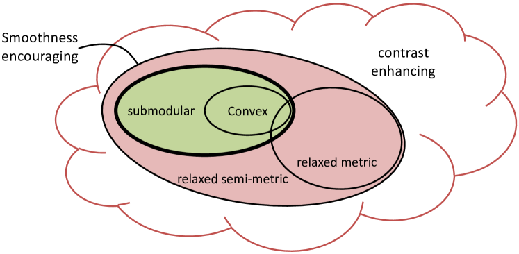
Figure 4: Different types of multilabel $F\left(\mathbf{x}\right)$: The hierarchy and relations between different types of multilabel energies. Green indicates the existence of global minimization algorithms. For energies in red there are good approximation algorithms.

convex	submodular	relaxed metric	relaxed semi-metric
$\ell_{1}$	$\ell_{1}$	truncated $\ell_{1}$	$\ell_{2}$
$\ell_{2}$	$\ell_{2}$	$\ell_{1}$	truncated $\ell_{2}$
		Potts

Table 2: examples of different types of pair-wise functions $\varphi_{ij}$

Unfortunately, the promising results of Schlesinger and Flach (2006) regarding the global minimization of submodular functions does not hold for more general functions. When $F\left(\mathbf{x}\right)$ is no longer submodular one can no longer hope to achieve global optimality in polynomial time. However, for relaxed metric and relaxed semi-metric functions Boykov et al. (2001) showed large move making approximate algorithms that performs quite well in practice (see e.g., Szeliski et al. (2008)). Large move making algorithms iteratively seek to improve the energy of a current solution by updating large number of variables at once. Each such large step is carried out by solving a simple binary submodular minimization via st-mincut. For relaxed metric functions the large move is $\alpha$-expansion. At each iteration a binary problem is solved: for each variable it can either retain its current label (0) or switch label to $\alpha$ (1). The relaxed metric property of $F\left(\mathbf{x}\right)$ ensures that the resulting binary problem is submodular and thus can be solved globally in polynomial time. The $\alpha$-expansion algorithm iterates over all labels until it converges. Convergence after finite number of iterations is guaranteed, and in certain cases some theoretical bounds can be proven on the quality of the approximation (see Boykov et al. (2001) for more details).

For relaxed semi-metric functions a slightly different large move is devised. For each pair of labels $\alpha$ and $\beta$ the large move is called $\alpha\beta$-swap. At each iteration a binary problem is solved for all variables currently labeled either $\alpha$ or $\beta$: for each variable it can pick either $\alpha$ (0) or $\beta$ (1). The relaxed semi-metric property of $F\left(\mathbf{x}\right)$ ensures that the resulting binary problem is submodular and thus can be solved globally in polynomial time. The $\alpha\beta$-swap algorithm iterates over all pairs of labels until it converges. Convergence after finite number of iterations is guaranteed, however, theoretical bounds on the approximation no longer exists (see Boykov et al. (2001) for more details). Table 3 shows the resulting types of pair-wise energies and the current results on their minimization. This thesis focuses on the hard optimization of the contrast-enhancing functionals defined on cyclic graphs. Part II shows how introducing energies that contain contrast-enhancing terms gives rise to new applications. While Part III deals with the methods of approximating these challenging contrast-enhancing energies.

	Tree	Cyclic
submodular	Easy: mincut, BP	Easy: mincut
semi-metric	Easy: BP	Good Approximations
contrast-enhancing	Easy: BP	Hard

Table 3: Hardness of optimization (multilabel): the computational “hardness” of discrete optimization as a function of the underlying graph structure and the class of pair-wise interactions.

5 Relation to Linear Programming (LP)

This section establishes a connection between the pair-wise energy minimization problem (10) and the field of convex optimization, in particular to Linear Programming (LP). For the following discussion it is useful to introduce some new notations and definitions. The first useful representation is the overcomplete representation of the solution vector $\mathbf{x}$. This representation is defined as follows Wainwright et al. (2005); Wainwright and Jordan (2008):

Definition 5.9 (Overcomplete representation).

A discrete solution $\mathbf{x}$ can be represented by an extended binary vector $\phi\left(\mathbf{x}\right)$, s.t.

$$\phi\left(\mathbf{x}\right)_{i,\alpha} = \delta\left(x_{i}==\alpha\right)$$ (16)

$$\phi\left(\mathbf{x}\right)_{ij,\alpha\beta} = \delta\left(x_{i}==\alpha\right)\cdot\delta\left(x_{j}==\beta\right)$$ (17)

where $\delta(\cdot)$ is the Kronecker delta function.

The overcomplete representation projects a discrete vector $\mathbf{x}$ of dimension $n$ into a $d$-dimensional binary vector $\phi\left(\mathbf{x}\right)$. The index set of vector $\phi\left(\mathbf{x}\right)$ is defined as $\mathcal{I}=\left\{i,\alpha\right\}\cup\left\{ij,\alpha\beta\right\}$, with $d=\left|\mathcal{I}\right|$.

With the overcomplete representation in mind, it is useful to parameterize the discrete function $F\left(\mathbf{x}\right)$ of Eq. (1) using a parameter vector $\theta$:

$$\theta_{i,\alpha}=\varphi_{i}\left(\alpha\right)$$ (18a)

$$\theta_{ij,\alpha\beta}=\varphi_{ij}\left(\alpha,\beta\right)$$ (18b)

Combining Def. 5.9 with the parametrization of (18b), the functional of Eq. (1) becomes

$$F\left(\mathbf{x}\right) = \sum_{i,\alpha}\theta_{i,\alpha}\phi\left(\mathbf{x}\right)_{i,\alpha}+\sum_{ij,\alpha\beta}\theta_{ij,\alpha\beta}\phi\left(\mathbf{x}\right)_{ij,\alpha\beta}$$ (19)

$$= \left<{\theta},{\phi\left(\mathbf{x}\right)}\right>$$

The overcomplete representation $\phi\left(\mathbf{x}\right)$ is defined over a discrete set of points. However, it is useful to consider a relaxation of this set into a convex continuous domains.

The tightest relaxation of the discrete set $\left\{\phi\left(\mathbf{x}\right)|\mathbf{x}\in\left\{1,\ldots,l\right\}^{n}\right\}$ is the marginal polytop $\mathbb{M}\left({\mbox{$\mathcal{E}$}}\right)$:

Definition 5.10 (Marginal polytop).

The marginal polytop of $F\left(\mathbf{x}\right)$ is the convex combination of the vertices $\phi\left(\mathbf{x}\right)$ for the $l^{n}$ discrete solutions $\mathbf{x}$. This set is formally defined as:

$$\mathbb{M}\left({\mbox{$\mathcal{E}$}}\right)=\left\{\mu\in\mathbb{R}^{d}\left|\mu=\sum_{\mathbf{x}}p\left(\mathbf{x}\right)\phi\left(\mathbf{x}\right),\;\mbox{for some distribution $p\left(\cdot\right)$}\right.\right\}$$ (20)

This marginal polytop, $\mathbb{M}\left({\mbox{$\mathcal{E}$}}\right)$, is defined by finite, yet exponentially large, number of half-spaces. Therefore, it is convenient to define a relaxed version of the marginal polytop:

Definition 5.11 (Local polytop).

The local polytop of $F\left(\mathbf{x}\right)$ is the convex set:

$$\mathbb{L}\left({\mbox{$\mathcal{E}$}}\right)=\left\{\tau\in\mathbb{R}^{d}\left|\begin{array}[]{rl}\sum_{\alpha}\tau_{i,\alpha}=1&\forall i\\ \sum_{\alpha\beta}\tau_{ij,\alpha\beta}=1&\forall ij\in\mbox{$\mathcal{E}$}\\ \sum_{\beta}\tau_{ij,\alpha\beta}=\tau_{i,\alpha}&\forall ij\in\mbox{$\mathcal{E}$},\beta\end{array}\right.\right\}$$ (21)

Unlike the marginal polytop, $\mathbb{L}\left({\mbox{$\mathcal{E}$}}\right)$ is defined using only polynomial number of half-spaces, and therefore it admits polynomial time optimization schemes. In fact, $\mathbb{L}\left({\mbox{$\mathcal{E}$}}\right)$ is the first order approximation of $\mathbb{M}\left({\mbox{$\mathcal{E}$}}\right)$ (Wainwright and Jordan (2008)).

Note that the geometry of $\mathbb{M}\left({\mbox{$\mathcal{E}$}}\right)$ and $\mathbb{L}\left({\mbox{$\mathcal{E}$}}\right)$ are affected by the number of variables $n$, the number of states $l$ and by the underlying graph structure $\mathcal{E}$ defining the interacting pairs of variables. These polytops are not affected by the parameters of $\varphi_{i}$ and $\varphi_{ij}$.

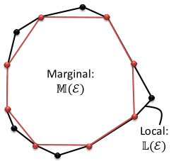
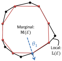
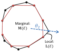
(a)	(b)	(c)

Figure 5: The Marginal and Local polytops: An illustration of the marginal, $\mathbb{M}\left({\mbox{$\mathcal{E}$}}\right)$, and local, $\mathbb{L}\left({\mbox{$\mathcal{E}$}}\right)$, polytops. (a) $\mathbb{L}\left({\mbox{$\mathcal{E}$}}\right)$ is an outer bound on the exact constraints of $\mathbb{M}\left({\mbox{$\mathcal{E}$}}\right)$. The vertex set of $\mathbb{L}\left({\mbox{$\mathcal{E}$}}\right)$ includes all integral vertices of $\mathbb{M}\left({\mbox{$\mathcal{E}$}}\right)$ (marked in red) . It also includes fractional vertices (marked in black), which are not vertices of $\mathbb{M}\left({\mbox{$\mathcal{E}$}}\right)$. (b), (c) Solving an LP with cost vector $\theta$ entails translating a hyperplane with normal $\theta$ until it is tangent to the constraint set. In (b) the point of tangency of cost vector $\theta_{1}$ occurs at an integral vertex. In (c) the point of tangency of cost vector $\theta_{2}$ occurs at a fractional vertex, outside $\mathbb{M}\left({\mbox{$\mathcal{E}$}}\right)$. In this case, there is an integrality gap. (figure taken from Wainwright et al. (2005)).

By standard properties of LP, the optimal value is attained at an extreme point of the constraint set (a vertex of the constraints polytop). The marginal polytop, $\mathbb{M}\left({\mbox{$\mathcal{E}$}}\right)$, is a convex set defined by all the possible solutions $\phi\left(\mathbf{x}\right)$. Hence, a vertex of $\mathbb{M}\left({\mbox{$\mathcal{E}$}}\right)$ corresponds to a vector $\phi\left(\mathbf{x}\right)$ for some discrete solution $\mathbf{x}$. We refer to these vertices as integral vertices corresponding to integral solutions of the LP. On the other hand, the local polytop, $\mathbb{L}\left({\mbox{$\mathcal{E}$}}\right)$, may contain more vertices that do not correspond to any discrete solution, $\mathbf{x}$. We refer to these vertices as fractional solutions. Fig. 5 provides an illustration of the marginal and local polytops, the relation between them, and their impact on the optimal solution of LP. The figure also distinguishes between the integral and fractional vertices of the polytops. (Wainwright et al., 2005, Example 3) describes in detail a case where fractional solution is optimal. It is important to note that the parameter vector $\theta$ for which the fractional solution is optimal, in their example, is such that encourages contrast between variables (i.e., $x_{i}\neq x_{j}$ for neighboring $i$ and $j$).

The relation between discrete energy minimization (problem (10)) and convex LP presented in this section lies in the foundation of popular optimization algorithms such as tree-reweighted BP (see Sec. 6.3). This relation is also important to illustrate the challenging task of optimizing (10): When $\theta$ represents an energy function that is “smoothness-encouraging” its optimal value usually corresponds to an integral vertex of $\mathbb{L}\left({\mbox{$\mathcal{E}$}}\right)$ and thus its optimization can be done exactly via LP over the relaxed constraint set $\mathbb{L}\left({\mbox{$\mathcal{E}$}}\right)$. However, when the energy has contrast-enhancing terms its optimal solution w.r.t $\mathbb{L}\left({\mbox{$\mathcal{E}$}}\right)$ is fractional – the global integral solution cannot be attained using the relaxed constraints of $\mathbb{L}\left({\mbox{$\mathcal{E}$}}\right)$. Therefore, the optimization of energies that have contrast-enhancing terms, is a very challenging task. This thesis focuses on these energies and proposes methods to cope with this inherent difficulty.

6 Discrete Optimization Algorithms

In the previous sections we outlined some key properties of the energy function $F\left(\mathbf{x}\right)$ and their effect on the minimization process. We also demonstrated how specific optimization algorithms take advantage of these properties. In this section we present several prominent optimization algorithms that we refer to later on in this thesis. These selected representative approaches sketches the main directions at which current discrete optimization research is mainly focused.

6.1 Iterated Conditional Modes (ICM)

ICM is a very simple and basic iterative optimization algorithm proposed by Besag (1986). It is an approximate method, acting locally on the variables, suitable for multilabel functions with arbitrary underlying graph and arbitrary $\varphi_{ij}$. At each iteration ICM visits all the variables sequentially, and choose for each variable the best state (with the lower energy) given the current states of all other variables. This process can be viewed as a greedy coordinate descend algorithm and it bears some analogy to Gauss-Seidel relaxations of the continuous domain (Varga (1962)).

ICM is a local update process and therefore is prone to getting stuck very fast in local minimum. It is also extremely sensitive to initialization (see e.g., Szeliski et al. (2008)).

When taking a probabilistic point of view, and considering the energy function as a Gibbs energy, that is representing some measure over all possible solutions:

$$Pr\left(\mathbf{x}\right)\propto\exp\left(-\frac{1}{T}F\left(\mathbf{x}\right)\right)$$ (22)

ICM may be viewed as a Gibbs sampler at the temperature limit $T\rightarrow 0$. Therefore, its performance is expected to be inferior to more sophisticated sampling methods such as, e.g., simulated annealing (Kirkpatrick et al. (1983)).

6.2 Belief Propagation (BP)

Belief-propagation is an optimization algorithm based on local updates. However, in contrast to the hard assignment ICM performs at each update, BP maintains “soft” beliefs for each variable and passes messages between neighboring variables according to their current belief. A message from variable $i$ to its neighbor $j$, $m_{i\rightarrow j}$, is a vector of length $L$. That is, the message vector encodes how $i$ “feels” about assigning state $\alpha$ to $j$.

$$m_{i\rightarrow j}\left(\alpha\right)=\min_{\beta}\left\{\varphi_{i}\left(\beta\right)+\sum_{ki\in\mbox{$\mathcal{E}$},k\neq j}m_{k\rightarrow i}\left(\beta\right)+\varphi_{ij}\left(\beta,\alpha\right)\right\}$$ (23)

The belief of each variable $i$ is also a vector of length $L$ encoding the tendency of $i$ to be assigned to state $\alpha$:

$$b_{i}\left(\alpha\right)=\varphi_{i}\left(\alpha\right)+\sum_{ki\in\mbox{$\mathcal{E}$}}m_{k\rightarrow i}\left(\alpha\right)$$ (24)

BP iteratively passes messages and updates the local belief for each variable. After its final iteration, each variable is assigned the label with the lowest energy, i.e., $x_{i}=\arg\min_{\alpha}b_{i}(\alpha)$.

Originally, BP was used as an inference algorithm in tree-structured graphical models (Pearl (1988); Koller and Friedman (2009)). Messages were initialized to zero. Then messages were passed from leafs to root and back to the leafs. This forward-backward message passing converges to the global optimum when $\mathcal{E}$ is a tree, regardless of the type of $\varphi_{ij}$ that can be arbitrary.

When the underlying graph $\mathcal{E}$ has cycles, BP is no longer guaranteed to converge. It was proposed to run BP on cyclic graphs, a variant called loopy-BP. In the loopy case, however, it is not clear how to schedule the messages and how to determine the number of iterations to perform. Even if the loopy BP converges to some fixed point, it is usually a local optimum with no guarantees on global optimality (Koller and Friedman (2009); Wainwright and Jordan (2008))

6.3 Tree-reweighted Belief Propagation (TRW)

A significant development of BP was presented in the works of Wainwright et al. (2005); Kolmogorov (2006); Werner (2007); Wainwright and Jordan (2008); Komodakis et al. (2011). These works proposed a new interpretation to the basic message passing operation that BP conducts. They relaxed the discrete minimization of $F\left(\mathbf{x}\right)$ to form a continuous linear programming (LP), in the same manner that was presented in Sec. 5. Then they related message passing to the optimization of the resulting LP. a It was shown that the relaxation of $F\left(\mathbf{x}\right)$ forms an LP with very specific structure. This special structure can, in turn, be exploited to devise a specially tailored optimization scheme that uses message passing as a basic operation.

The tree-reweighted BP approach establishes a relation between discrete optimization and continuous convex optimization of LP. This relation brings forward interesting results and properties from the continuous optimization domain to the discrete one. For instance, it allows to use Lagrangian multipliers and formulate a Lagrangian dual to the original problem. The dual representation provides a lower bound to the sought optimal solution. If a solution $\mathbf{x}^{\star}$ is found with an energy $F\left(\mathbf{x}^{\star}\right)$ equals to the lower bound, then a certificate is provided that this $\mathbf{x}^{\star}$ is a global minimum.

It was shown (e.g., Szeliski et al. (2008)) that in practice in many computer vision application TRW was able to recover globally optimal solutions. These results dealt mainly with relaxed metric energies (see Sec. 4). However, there is no general guarantee on TRW and there are cases involving challenging energies, beyond relaxed metric, for which it was shown that an integrality gap exists and TRW can no longer provide a tight approximation (e.g., Kolmogorov (2006); Bagon and Galun (2011)).

6.4 Large Move Methods

As opposed to local methods such as ICM, BP and TRW, there is the approach of Boykov et al. (2001) that proposes discrete methods based on combinatorial principles. The basic observation that lies at the heart of the large-move algorithms is that instead of treating the variables locally one at a time, one may affect the labeling of many variables at once by performing large moves. These large moves are formulated as a binary step, and the difference between the different “flavors” of the large-move algorithms is the formulation of these binary steps. What makes these large move effective and efficient is the fact that binary submodular sub-problems can be solved globally and efficiently.

The two basic large move algorithms, $\alpha$-expand and $\alpha\beta$-swap, were already described in Sec. 4 in the context of relaxed metric and relaxed semi metric energies. Recently, another large move making algorithm called fusion-moves was proposed (Lempitsky et al. (2007, 2010)) At each iteration of the fusion algorithm a discrete solution is proposed. The proposed solution is fused into the current solution via a binary optimization: each variable can retain its current label ($0$), or switch to the respective label from the proposed solution ($1$). However, unlike the swap and expand algorithms, the resulting binary optimization of the fusion step is no longer guaranteed to be submodular and highly depends on the types of proposed solutions. Therefore, it is often the case that QPBO (Kolmogorov and Rother (2007)), which is a non-submodular binary approximation algorithm, is used to perform the binary steps of the fusion algorithm.

To summarize this brief outline of existing approximation algorithms one may notice that a lot of effort is put in recent years in developing and improving approximate optimization algorithms. Research is put into both providing better practical results and into exploring the theoretic aspects of the problem. Approximation methods are derived and inspired by both the continuous optimization domain (e.g., TRW) and the discrete domain (e.g., graph-cuts). However, these results mainly focus on the minimization of functions $F\left(\mathbf{x}\right)$ that have some structure to them: either relaxed metric or relaxed semi-metric (see, for example, the survey of Szeliski et al. (2008)). For these smoothness-encouraging functions current algorithms succeed in providing good approximations in practice, despite their theoretical NP-hardness. In contrast, when it comes to arbitrary, contrast-enhancing functions, little is known in terms of approximation and no method currently exists (to the best of our knowledge) that provides satisfying approximations. This thesis focuses on the optimization of arbitrary, contrast-enhancing functions.

Chapter 2 Outline of this Thesis

Discrete energy minimization is a ubiquitous task in computer vision and in other scientific domains. However, in the previous chapter we saw that the optimization of such discrete energies is known to be NP-hard in most cases (Boykov et al. (2001)). Despite this theoretical hardness, for many “smoothness encouraging” energies (relaxed semi-metric), approximate optimization algorithms exist and provide remarkable approximations in practice.

However, as tasks become more sophisticated, the models grow more complex: From tree structured to cyclic graphs and grids, and from simple smoothing priors to complex arbitrary pair-wise interactions. As the energies become less constrained and structured one gains more expressive power for the objective function at the cost of a significantly more challenging optimization task.

In this work I would like to step outside this “comfort-zone” of the smoothness-encouraging energies and explore more challenging discrete energies. This step gives rise to two important questions:

1. Why bother? Why should one consider energy functions beyond semi-metric? What can be gained (in term of expressive power) considering the significant hardness of the entailed optimization task?

2. In case we decide to embark on this challenging task of approximating arbitrary discrete energy, how can we tackle this problem? Can we propose new approaches and directions for the difficult approximation tasks of discrete energies, beyond semi-metric?

These two research questions provide the road map of this thesis. Consequently, this thesis revolves around two major axes: applications and approximations.

Applications

The first axis of this thesis involves exploring new applications that require arbitrary, contrast-enhancing energies beyond semi-metrics. These examples demonstrate how the additional expressive power of arbitrary energies is crucial to derive new applications. We show how utilizing arbitrary energies gives rise to interesting and desirable behaviors for different applications. We present these new applications in Part II of this thesis.

Chapter 3 shows an image sketching application that provides a binary sketch from a small collection of images of similar objects. In this application the binary sketch is described via the interactions between neighboring pixels in the corresponding images. Neighboring sketch bits corresponding to similar image pixels are encourage to have similar value (i.e., submodular, smoothness-enhancing term). In contrast, neighboring sketch bits corresponding to dissimilar image pixels are encourage to have different value (i.e., non-submodular, contrast-enhancing term). The binary sketch is then the output of the resulting non-submodular energy minimization.

The sketching application may be thought of as a special case of binary image segmentation. Considering contrast-enhancing objective function for the task of unsupervised segmentation or clustering may introduce a solution not only to the clustering problem, but also may help in determining the underlying number of clusters. This clustering objective function is commonly known as “Correlation Clustering” (Bansal et al. (2004)). Chapter 4 explores the Correlation Clustering functional and its underlying “model-selection” capability.

Image segmentation and clustering are not the only examples for contrast-enhancing energies. Chapter 5 describes a 3D surface reconstruction from multiple images under different known lighting. The reconstruction takes into account the changes in appearance of the surface due to the change in lighting directions. These changes amounts to an implicit partial differential equation (PDE) that describes the unknown surface. In this work we propose to pose the solution of the resulting PDE as a discrete optimization task. Incorporating integrability prior on the unknown surface, the resulting discrete energy has contrast-enhancing terms.

Modeling and prior knowledge are not the only sources for contrast-enhancing terms in energies. In many cases, the exact parameters of an energy are learned from training data. Chapter 6 presents Decision Tree Fields (DTF): an example of such a learning scheme. DTF learns, in a principled manner, a pair-wise energy from labeled training examples. Since the learning process is not constraint to smoothness-encouraging energies, it is often the case that the resulting energy has contrast-enhancing terms. In its training phase DTF seeks parameters that (approximately) maximize the likelihood of the data. Therefore, the resulting contrast-enhancing terms are better suited to describe the underlying “behavior” of the data. Restricting the model to smoothness-encouraging terms only would prohibit DTF from accurately predicting results at test time.

Approximate Optimization

The enhancement in descriptive power gained by considering arbitrary energies comes with a price tag: we no longer have good approximation algorithms at hand. Therefore, the second axis of this thesis explores possible directions for approximating the resulting challenging arbitrary energies. In part III of this work I propose practical methods and approaches to approximate the resulting NP-hard optimization problems. In particular, in Chapter 7, I propose a discrete optimization approach to the aforementioned correlation clustering optimization. This approach scales gracefully with the number of variables, better than existing approaches (e.g., Vitaladevuni and Basri (2010)).

Chapter 8 concludes this part with a more general perspective on discrete optimization. This new perspective is inspired by multiscale approaches and suggests to cope with the NP-hardness of discrete optimization using the multiscale landscape of the energy function. Defining and observing this multiscale landscape of the energy, I propose methods to explore and exploit it to derive a coarse-to-fine optimization framework. This new perspective gives rise to a unified multiscale framework for discrete optimization. Our proposed multiscale approach is applicable to a diversity of discrete energies, both smoothness-encouraging as well as arbitrary, contrast-enhancing functions.

Part II Applications

This part concentrate on the first axis of this thesis. This direction explores new applications which require arbitrary energies. We start with an unsupervised clustering objective function, Correlation Clustering (CC). Chapters 3 and 4 show several applications all revolving around the correlation clustering energy. This energy is hard to optimize: It has both smoothness-encouraging as well as contrastive pair-wise terms; it has no data term to guide the optimization process, and the number of discrete labels is not known a-priori. We analyze an interesting property of the correlation clustering functional: its ability to recover the underlying number of clusters. This interesting property is due mainly to the usage of terms that enhance contrast, rather than smoothness, in the solution $\mathbf{x}$.

Another application that requires arbitrary energy is 3D reconstruction of surfaces. We show, in chapter 5, how under certain conditions 3D reconstruction may be posed as a solution to a partial differential equation (PDE). Solving this PDE to recover the 3D surface can be done through discretization of the solution space. The discrete version of the PDE yields pair-wise terms that are beyond semi-metric.

Finally, the parameters of the energy function defining the terms $\varphi_{i}$ and $\varphi_{ij}$ may not be fixed a-priori. It may happen that one would like to learn the energy function from training data for various applications. Chapter 6 shows an example of such an energy learning framework. The resulting learned energy is no longer guaranteed to be “well-behaved”. In fact, experiments show that when the learning procedure is not constrained it is often the case that the resulting energy is arbitrary and does not yield any known structure.

Chapter 3 Sketching the Common

Given very few images containing a common object of interest under severe variations in appearance, we detect the common object and provide a compact visual representation of that object, depicted by a binary sketch. Our algorithm is composed of two stages: (i) Detect a mutually common (yet non-trivial) ensemble of ‘self-similarity descriptors’ shared by all the input images.  (ii) Having found such a mutually common ensemble, ‘invert’ it to generate a compact sketch which best represents this ensemble. This provides a simple and compact visual representation of the common object, while eliminating the background clutter of the query images. It can be obtained from very few query images. Such clean sketches may be useful for detection, retrieval, recognition, co-segmentation, and for artistic graphical purposes.

The ‘inversion’ process that generates the sketch is formulated as a discrete optimization problem of a binary, non-submodular energy function.

7 Introduction

Given very few images (e.g., 3-5) containing a common object of interest, possibly under severe appearance changes, we detect the common object and provide a simple and compact visual representation of that object, depicted by a binary sketch (see Fig. 6). The input images may contain additional distracting objects and clutter, the object of interest is at unknown image locations, and its appearance may significantly vary across the images (different colors, different textures, and small non-rigid deformations). We do assume, however, that the different instances of the object share a very rough common geometric shape, of roughly the same scale ($\pm 20\%$) and orientation ($\pm 15^{\circ}$). Our output sketch captures this rough common shape.

The need to extract the common of very few images occurs in various application areas, including:  (i) object detection in large digital libraries. For example, a user may provide very few (e.g., 3) example images containing an object of interest with varying appearances, and wants to retrieve new images containing this object from a database, or from the web.  (ii)  Co-segmentation of a few images.  (iii) Artistic graphical uses.

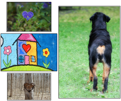
(a)  (b)

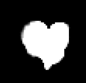
Figure 6: Detecting and sketching the common: (a) The 4 input images provided to the algorithm. (b) The least trivial common part (the heart) is detected and sketched by the algorithm.

Our method is based on densely computed Local Self-Similarity Descriptors Shechtman and Irani (2007). Our algorithm is composed of two main steps: (i) Identify the common object by detecting a similar (yet “non-trivial”) ensemble of self-similarity descriptors, that is shared by all the input images. Corresponding descriptors of the common object across the different images should be similar in their descriptor values, as well as in their relative positions within the ensemble. (ii) Having found such a mutually common ensemble of descriptors, our method “inverts” it to generate a compact binary sketch which best represents this ensemble.

It was shown in Shechtman and Irani (2007) that given a single query image of an object of interest (with very little background clutter), it is possible to detect other instances of that object in other images by densely computing and matching their local self-similarity descriptors. The query image can be a real or synthetic image, or even a hand-drawn sketch of the object.

In this paper we extend the method of Shechtman and Irani (2007) to handle multiple query images. Moreover, in our case those images are not centered around the object of interest (its position is unknown), and may contain also other objects and significant background clutter. Our goal is to detect the “least trivial” common part in those query images, and generate as clean as possible (region-based) sketch of it, while eliminating the background clutter of the query images. Such clean sketches can be obtained from very few query images, and may be useful for detection, retrieval, recognition, and for artistic graphical purposes. Some of these applications are illustrated in our experiments.

Moreover, while Shechtman and Irani (2007) received as an input a clean hand-drawn sketch of the object of interest (and used it for detecting other instances of that object), we produce a sketch as one of our outputs, thereby also solving the “inverse” problem, namely: Given several images of an object, we can generate its sketch using the self-similarity descriptor.

A closely related research area to the problem we address is that of ’learning appearance models’ of an object category, an area which has recently received growing attention (e.g., Chum and Zisserman (2007); Chum et al. (2009); Ferrari et al. (2009); Winn and Jojic (2005); Karlinsky et al. (2008); Lee and Grauman (2009); Nguyen et al. (2009); Wu et al. (2009); Zhu et al. (2008), to name just a few). The goal of these methods is to discover common object shapes within collections of images. Some methods assume a single object category (e.g., Chum and Zisserman (2007); Ferrari et al. (2009); Karlinsky et al. (2008); Winn and Jojic (2005); Nguyen et al. (2009); Wu et al. (2009); Zhu et al. (2008)), while others assume multiple object categories (e.g., Chum et al. (2009); Lee and Grauman (2009)). These methods, which rely on weakly supervised learning (WSL) techniques, typically require tens of images in order to learn, detect and represent an object category. What is unique to the problem we pose and to our method is the ability to depict the common object from very few images, despite the large variability in its appearance. This is a scenario no WSL method (nor any other method, to our best knowledge) is able to address. Such a small number of images (e.g., $3$) does not provide enough ’statistical samples’ for WSL methods. While our method cannot compete with the performance of WSL methods when many (e.g., tens) of example images are provided, it outperforms existing methods when only few images with large variability are available. We attribute the strength of our method to the use of densely computed region-based information (captured by the local self-similarity descriptors), as opposed to commonly used sparse and spurious edge-based information (e.g., gradient-based features, SIFT descriptors, etc.) Moreover, the sketching step in our algorithm provides an additional global constraint.

Another closely related research area to the problem addressed here is ‘co-segmentation’ (e.g., Rother et al. (2004b); Bagon et al. (2008); Mukherjee et al. (2009)). The aim of co-segmentation is to segment out an object common to a few images ($2$ or more), by seeking segments in the different images that share common properties (colors, textures, etc.) These common properties are not shared by the remaining backgrounds in the different images. While co-segmentation methods extract the common object from very few images, they usually assume a much higher degree of similarity in appearance between the different instances of the object than that assumed here (e.g., they usually assume similar color distributions, similar textures, etc.)

The rest of the paper is organized as follows: Sec. 8 formulates the problem and gives an overview of our approach. Sec. 9 describes the component of our algorithm which detects the ‘least trivial’ common part in a collection of images, whereas Sec. 10 describes the sketching component of our algorithm. Experimental results are presented in Sec. 11.

8 Problem Formulation

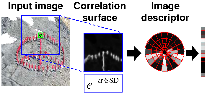
Figure 7: The Local Self Similarity Descriptor: (Figure taken from Shechtman and Irani (2007).)  The self-similarity descriptor for any given point (e.g., the green point in the left image), is computed by measuring the similarity of a $5\times 5$ patch around the point with the surrounding $60\times 60$ image region. This results in a ‘correlation’ surface (middle image). The correlation surface is quantized into a compact log-polar representation of 45 bins (15 angles, 3 radial intervals) to achieve invariance against small local affine and non-rigid deformations. The maximum value in each bin constitutes the value at the corresponding descriptor entry (right most image).

Let $I_{1},...,I_{K}$ be $K$ input images containing a common object under widely different appearances. The object may appear in different colors, different textures, and under small non-rigid deformations. The backgrounds are arbitrary and contain distracting clutter. The images may be of different sizes, and the image locations of the common object are unknown. We do assume, however, that the different instances of the object share a very rough common geometric shape, of roughly the same scale and orientation. Our output sketch captures this rough common shape.

Our approach is thus based on detecting ’common regions’ (as opposed to ’common edges’), using densely computed Local Self-Similarity Descriptors Shechtman and Irani (2007). This descriptor (illustrated in Fig. 7) captures local shape information in the image vicinity where it is computed, while being invariant to its photometric properties (color, texture, etc.) Its log-polar representation makes this descriptor insensitive to small affine and non-rigid deformations (up to $\pm 20\%$ in scale, and $\pm 15^{\circ}$). It was further shown by Hörster et al. (2008) that the local self-similarity descriptor has a strong descriptive power (outperforming SIFT). The use of local self-similarity descriptors allows our method to handle much stronger variations in appearance (and in much fewer images) than those handled by previous methods. We densely compute the self-similarity descriptors in images $I_{1},...,I_{K}$ (at every $5$-th pixel). ‘Common’ image parts across the images will have similar arrangements of self similarity descriptors.

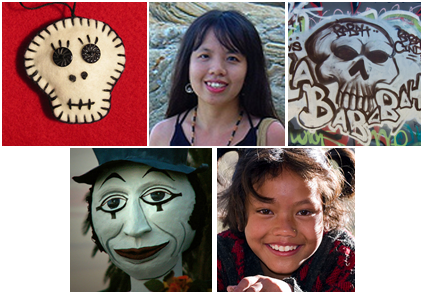
(a) (b)

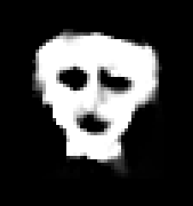
Figure 8: Sketching:  (a) Five input images.   (b) Their joint sketch.

Let $c_{1},...,c_{K}$ denote the unknown locations of the common object in the $K$ images. Let $I_{k}^{c_{k}}$ denote a $w\times h$ subimage of $I_{k}$ centered at $c_{k}$, containing the common object ($k=1,...,K$) (need not be tight). For short, we will denote it by $\tilde{I_{k}}$. The sketch we seek is a binary image $S$ of size $w\times h$ which best captures the rough characteristic shape of the common object shared by $\tilde{I_{1}},...,\tilde{I_{K}}$. More formally, we seek a binary image $S$ whose local self-similarity descriptors match as best as possible the local self-similarity descriptors of $\tilde{I_{1}},...,\tilde{I_{K}}$. The descriptors should match in their descriptor values, as well as in their relative positions with respect to the centers $\{c_{k}\}$:

$$Score(S|\tilde{I_{1}},...,\tilde{I_{K}}) = \sum_{k=1}^{K}match(S,\tilde{I_{k}})$$

$$= \sum_{k=1}^{K}\sum_{i=1}^{w\cdot h}sim\left(d_{i}^{S},d_{i}^{k}\right)$$

where $d_{i}^{S}$ is the $i$-th self-similarity descriptor computed at image location $l_{i}$ in the sketch image $S$, $d_{i}^{k}$ is the self-similarity descriptor computed at the same relative position $l_{i}$ (up to small shifts) in the $w\times h$ subimage $\tilde{I_{k}}$, and $sim(d_{1},d_{2})=-\parallel d_{1}-d_{2}\parallel_{p}$ measures how similar two descriptor vectors are (we experimented with $L_{p}$ norms for $p=1,2$). Thus, the binary sketch we seek is:

$$\hat{S}=argmax\{Score(S|\tilde{I_{1}},...,\tilde{I_{K}})\}\ \ s.t.\ \ S(l)\in\{-1,1\}$$ (26)

where $S(l)$ is the value of $S$ at pixel $l$. This process is described in detail in Sec. 10, and results in a sketch of the type shown in Fig 8.

While edge-based detection and/or sketching Lee and Grauman (2009); Zhu et al. (2008); Ferrari et al. (2009) requires many input images, our region-based detection and sketching can be recovered from very few images. Edges tend to be very spurious, and are very prone to clutter (even sophisticated edge detectors like Maire et al. (2008) – see Fig. 9.b). Edge-based approaches thus require a considerable number of images, to allow for the consistent edge/gradient features of the object to stand out from the inconsistent background clutter. In contrast, region-based information is much less sparse (area vs. line-contour), less affected by clutter or by misalignments, and is not as sensitive to the existence of strong clear boundaries. Much larger image offsets are required to push two corresponding regions out of alignment than to misalign two thin edges. Thus, region-based cues require fewer images to detect and represent the common object. Indeed, our method can provide good sketches from as few as $3$ images. In fact, in some cases our method produces a meaningful sketch even from a single image, where edge-based sketching is impossible to interpret – see example in Fig. 9.

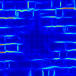
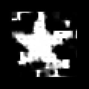
(a)	(b)	(c)

Figure 9: Regions vs. Edges:  (a) a single input image.  (b) The edge map generated by the method of Maire et al. (2008).  (c) The binary sketch generated by our method when applied to the single input image (using all the self-similarity descriptors densely computed in that image).  This illustrates the concept that region-based information is much richer than sparse edge-based information, and therefore appears to be more powerful for detection and for sketching.

In the general case, however, the locations $c_{1},...,c_{K}$ of the object within the input images $I_{1},...,I_{K}$, are unknown. We seek a binary image $S$ which sketches the ‘least trivial’ object (or image part) that is ‘most common’ to all those images. The ‘most common’ constraint is obvious: in each image $I_{k}$ there should be a location $c_{k}$ for which  $match\left(S,I_{k}^{c_{k}}\right)$  is high (where $\tilde{I_{k}}=I_{k}^{c_{k}}$ is the subimage centered at $c_{k}$).  However, there are many image regions that are trivially shared by many natural images. For example, uniform regions (of uniform color or uniform texture) occur abundantly in natural images. Such regions share similar self-similarity descriptors, even if the underlying textures or colors are different (due to the invariance properties of the self-similarity descriptor). Similarly, strong vertical or horizontal edges (e.g., at boundaries between two different uniformly colored/textured regions) occur abundantly in images. We do not wish to identify such trivial (insignificant) common regions in the images as the ‘common object’.

Luckily, since such regions have good image matches in lots of locations, the statistical significance of their good matches tends to be low (when measured by how many standard deviations its peak match values are away from its mean match value in the collection of images). In contrast, a non-trivial common part (with non-trivial structure) should have at least one good match in each input image (could also have a few matches in an image), but these matches would be ‘statistically significant’ (i.e., this part would not be found ‘at random’ in the collection of images).

Thus, in the general case, we seek a binary sketch $S$ and locations $c_{1},...,c_{K}$ in images $I_{1},...,I_{K}$, such that:

(i) $S$ is ‘most common’, in the sense that it maximizes $Score(S|I_{1}^{c_{1}},..,I_{K}^{c_{K}})=\sum_{k=1}^{K}match(S,I_{k}^{c_{k}})$ of Eq. (8).

(ii) $S$ is ‘least trivial’, in the sense that its matches at $c_{1},...,c_{K}$ are statistically significant, i.e., it maximizes $\sum_{k=1}^{K}StatSignificance\left(match(S,I_{k}^{c_{k}})\right)$,  where the significance of a match of $S$ is measured by how many standard deviations it is away from the mean match value of $S$.

Our optimization algorithm may iterate between these two constraints:   (i) Detect the locations $\{c_{k}\}_{k=1}^{K}$ of the least trivial common image part in $\{I_{k}\}_{k=1}^{K}$ (Sec. 9).  (ii) Sketch the common object given those image locations (Sec. 10).   The overall process results in a sketch image, which provides a simple compact visual representation of the common object of interest in a set of query images, while eliminating any distracting background clutter found in those images.

9 Detecting the Common

We wish to detect image locations $c_{1},...,c_{K}$ in $I_{1},...,I_{K}$, such that corresponding subimages centered at those locations, $I_{k}^{c_{k}}$, share as many self-similarity descriptors with each other as possible, yet their matches to each other are non-trivial (significant). The final sketch $S$ will then be obtained from those subimages (Sec. 10).

Let us first assume that the dimension $w\times h$ of the subimages is given. We will later relax this assumption. Let $\tilde{I}$ be a $w\times h$ image segment (this could be the final sketch $S$, or a subimage extracted from one of the $K$ input images in the iterative process). We wish to check if $\tilde{I}$ has a good match in each of the input images $I_{1},...,I_{K}$, and also check the statistical significance of its matches. We ‘correlate’ $\tilde{I}$ against all the input images (by measuring the similarity of its underlying self-similarity descriptors). In each image $I_{k}$ we find the highest match value of $\tilde{I}$: $maxMatch(\tilde{I},I_{k})$. The higher the value, the stronger the match. However, not every high match value is statistically significant. The statistical significance of $maxMatch(\tilde{I},I_{k})$ is measured by how many standard deviations it is away from the mean match value of $\tilde{I}$ in the entire collection of images, i.e.,:

$$\left(maxMatch(\tilde{I},I_{k})-avgMatch(\tilde{I})\right)/stdMatch(\tilde{I})$$

where $avgMatch(\tilde{I})$ is the mean of all match values of $\tilde{I}$ in the collection $I_{1},...,I_{K}$, and $stdMatch(\tilde{I})$ is their standard deviation. We thus define the ‘Significance’ of a subimage $\tilde{I}$ as:

$$Significance(\tilde{I}|I_{1},...,I_{K})=\frac{1}{K}\sum_{k=1}^{K}StatSignificance\left(maxMatch(\tilde{I},I_{k})\right)$$

Initially, we have no candidate sketch $S$. However, we can measure how ‘significantly common’ is each $w\times h$ subimage of $I_{1},...,I_{K}$, when matched against all locations in all the other $K-1$ images. We can assign a significance score to each pixel $p\in I_{k}$ ($k=1,..,K$), according to the ‘Significance’ of its surrounding $w\times h$ subimage: $Significance(I_{k}^{p}|I_{1},...,I_{K})$.

We set $c_{k}$ to be the pixel location with the highest significance score in image $I_{k}$, i.e., $c_{k}=argmax_{p\in I_{k}}\{Significance(I_{k}^{p}|I_{1},...,I_{K})\}$.

The resulting $K$ points (one per image), $c_{1},...,c_{K}$, provide the centers for $K$ candidates of ‘non-trivial’ common image parts. We generate a sketch $S$ from these image parts (using the algorithm of Sec. 10).

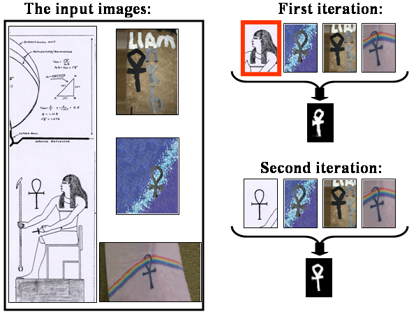
Figure 10: Iterations of Detection & Sketching: Left: The $4$ input images.  Right: The first iteration of the detection algorithm results in $4$ detected image regions, of which $3$ are correct and one is an outlier (marked by red). The resulting sketch produced from these regions is reasonably good (due to the robustness of the sketching to outliers – see Secs. 10 and 11), and is used for refining the detection in the input images. This results in $4$ correct detections in the second iteration, and an improved sketch.

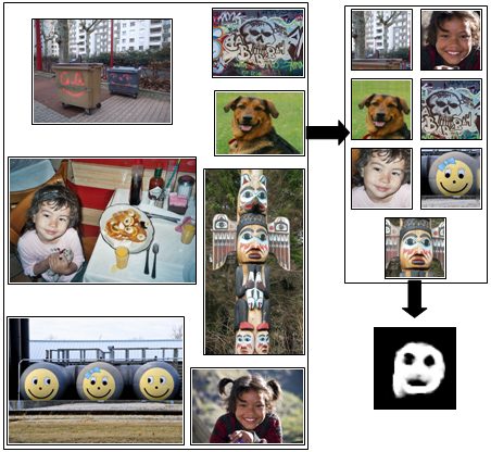
Figure 11: Detecting and sketching the common: (Left) The input images.   (Upper-Right) The detected image regions of the common object, including one outlier.   (Lower-Right) The resulting sketch.

We repeat the above process, this time for $\tilde{I}=S$, to detect its best matches in $I_{1},...,I_{K}$. This should lead to improved detection and localization of the common object ($c_{1},...,c_{K}$), and accordingly to an improved sketch $S$. This algorithm can be iterated several times. In practice, in all our experiments a good sketch $S$ was recovered already in the first iteration. An additional iteration was sometimes useful for improving the detection. Fig. 10 shows two iterations of this process, applied to $4$ input images. More results of the detection can be seen in Fig. 11.

Handling unknown w $\times$ h:   In principle, when $w\times h$ is unknown, we can run the above algorithm “exhaustively” for a variety of $w=w_{min},..,w_{max}$ and $h=h_{min},..,h_{max}$, and choose “the best” $w\times h$ (with maximal significance score). In practice, this is implemented more efficiently using “integral images”, by integrating the contributions of individual self-similarity descriptors into varying window sizes $w\times h$.

Computational Complexity:   The detection algorithm is implemented coarse-to-fine. The first step of the algorithm described above is quadratic in the size of the input images. However, since the number of images is typically small (e.g., $3-5$), and since the quadratic step occurs only in the coarsest/smallest resolutions of the images, this results in a computationally efficient algorithm.

10 Sketching the Common

Let $\tilde{I_{1}},\ldots,\tilde{I_{K}}$ be the $w\times h$ subimages centered around the common object (detected and extracted from the input images using the algorithm of Sec. 9). The goal of the sketching process is to produce a binary image $S$, which best captures the rough characteristic shape of the object shared by $\tilde{I_{1}},...,\tilde{I_{K}}$, as posed by Eq. (26). Namely, find $S$ whose ensemble of self-similarity descriptors is as similar as possible to the ensembles of descriptors extracted from $\tilde{I_{1}},\ldots,\tilde{I_{K}}$. If we were to neglect the binary constraint $S(l)\in\{-1,1\}$ in Eq. (26), and the requirement for consistency between descriptors of an image, then the optimal solution for the collection of self-similarity descriptors of $S$,  $\{d_{i}\}_{i=1}^{w\cdot h}$,  could be explicitly computed as:

$$d_{i}= \textmd{median}_{k}\{d_{i}^{k}\} \leavevmode\nobreak\ \leavevmode\nobreak\ \mbox{if }L_{1}\mbox{-norm}$$ (27)

$$d_{i}= \textmd{mean}_{k}\{d_{i}^{k}\} \leavevmode\nobreak\ \leavevmode\nobreak\ \mbox{if }L_{2}\mbox{-norm}$$

We use the $L_{1}$-norm to generate these ‘combined’ descriptors $\{d_{i}\}_{i=1}^{w\cdot h}$, because of the inherent robustness of the median operator to outliers in the descriptors (also confirmed by our empirical evaluations in Sec 11). Having recovered such a collection of descriptors for $S$, we proceed and solve the “inverse” problem – i.e., to generate the image $S$ from which these descriptors emanated. However, the collection of descriptors $\{d_{i}\}_{i=1}^{w\cdot h}$ generated via a ‘median’ or ‘average’ operations is no longer guaranteed to be a valid collection of self-similarity descriptors of any real image (binary or not). We thus proceed to recover the simplest possible image $S$ whose self-similarity descriptors best approximate the ‘combined’ descriptors $\{d_{i}\}_{i=1}^{w\cdot h}$ obtained by Eq. (27).

Self-similarity descriptors cover large image regions, with high overlaps. As such, the similarity and dissimilarity between two image locations (pixels) of $S$ are implicitly captured by multiple self-similarity descriptors and in different descriptor entries. The self-similarity descriptor as defined in Shechtman and Irani (2007) has values in the range $[0,1]$, where $1$ indicates high resemblance of the central patch to the patches in the corresponding log-polar bin, while $0$ indicates high dissimilarity of the central patch to the corresponding log-polar bin. For our purposes, we stretch the descriptor values to the range $[-1,1]$, where $1$ signifies “attraction” and $-1$ signifies “repulsion” between two image locations.

Let $W$ be a $wh\times wh$ matrix capturing the attraction/repulsion between every two image locations, as induced by the collection of the ‘combined’ self-similarity descriptors $\{d_{i}\}_{i=1}^{w\cdot h}$ of Eq. (27). Entry $w_{ij}$ in the matrix is the degree of attraction/repulsion between image locations $l_{i}$ and $l_{j}$, determined by the self-similarity descriptors $d_{i}$ and $d_{j}$ centered at those points. $d_{i}(l_{j})$ is the value of the bin containing location $l_{j}$ in descriptor $d_{i}$ (see Fig. 12). Similarly, $d_{j}(l_{i})$ is the value of the bin containing location $l_{i}$ in descriptor $d_{j}$. The entry $w_{ij}$ gets the following value:

$$w_{ij}=\alpha_{ij}\left(d_{i}(l_{j})+d_{j}(l_{i})\right)/2$$ (28)

where $\alpha_{ij}=\alpha_{ji}$ is inversely proportional to the distance $\parallel l_{i}-l_{j}\parallel$ between the two image locations (we give higher weight to bins that are closer to the center of the descriptor, since they contain more accurate/reliable information).

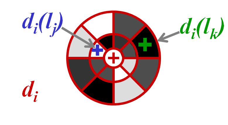
Figure 12: Computing attraction/repulsion matrix $W$: The log-polar self-similarity descriptor $d_{i}$ is located at $l_{i}$ (red cross). White bins signify image areas of high similarity to the central patch, dark bins signify image areas of dissimilarity to the central patch. The point $l_{j}$ (blue cross), which is the center of descriptor $d_{j}$ (not drawn), falls in a white bin of descriptor $d_{i}$ (i.e., $0<d_{i}(l_{j})\leq 1$). The entry $w_{ij}$ in the matrix $W$ is determined accordingly: $w_{ij}=\alpha_{ij}\left(d_{i}(l_{j})+d_{j}(l_{i})\right)/2$, where $\alpha_{ij}$ (the certainty assigned to this entry), is inversely proportional to the distance $\parallel l_{i}-l_{j}\parallel$ (the distance between the red and blue crosses). Similarly, the point $l_{k}$ (green cross), which is the center of another descriptor $d_{k}$ (also not drawn), falls in a dark bin of descriptor $d_{i}$, i.e., $-1\leq d_{i}(l_{k})<0$, and $\alpha_{ik}<\alpha_{ij}$ (because the green cross falls farther away from the center of $d_{i}$, hence lower certainty).

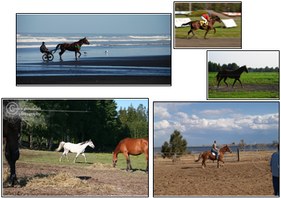
(a) (b)

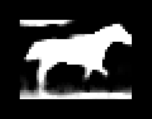
Figure 13: Detecting and sketching the common: (a) Five input images. (b) The resulting sketch.

Note that a ‘pure’ attraction/repulsion matrix $W$ of a true binary image $S$ contains only $3$ types of values $w_{ij}$: $-1,0,1$. If $l_{i}$ and $l_{j}$ belong to the same region in $S$ (i.e., both in foreground or both in background), then $w_{ij}=1$; if $l_{i}$ and $l_{j}$ belong to different regions in $S$, then $w_{ij}=-1$, and if the points are distant (out of descriptor range), then $w_{ij}=0$. In the general case, however, the entries span the range $[-1,1]$, where $1$ stands for “strong” attraction, $-1$ for “strong” repulsion and $0$ means “don’t care”. The closer the value of $w_{ij}$ to $0$, the lower its attraction/repulsion confidence; the closer it is to $\pm 1$, the higher the attraction/repulsion confidence.

Note that $W$ is different from the classical affinity matrix used in spectral clustering or in min-cut, which use non-negative affinities, and their value $0$ is ambiguous – it signifies both high-dissimilarity as well as low-confidence. The distinction between ‘attraction’, ‘repulsion’, and ‘low-confidence’ is critical in our case, thus we cannot resort to the max-flow algorithm or to spectral clustering in order to solve our problem. An affinity matrix with positive and negative values was used by Yu and Shi (2001) in the context of the normalized-cut functional. However, their functional is not appropriate for our problem (and indeed did not yield good results for $S$ when applied to our $W$). We therefore define a different functional and optimization algorithm in order to solve for the binary sketch $S$.

The binary image $S$ which best approximates the attraction/repulsion relations captured by $W$, will minimize the following functional:

$$\min_{S}\sum_{i,j}w_{ij}(S(l_{i})-S(l_{j}))^{2}\leavevmode\nobreak\ \leavevmode\nobreak\ \leavevmode\nobreak\ \leavevmode\nobreak\ \leavevmode\nobreak\ \mbox{subject to}\leavevmode\nobreak\ \leavevmode\nobreak\ S(l)\in\{-1,1\}$$ (29)

where $S(l)$ is the value of $S$ at pixel $l$. Note that for a binary image, the term $(S(l_{i})-S(l_{j}))^{2}$ can obtain only one of two values: $0$ (if both pixels belong to foreground, or both belong to background), or   $4$ (if one belongs to the foreground, and one to the background). Thus, when $w_{ij}$ is positive (attraction), $S(l_{i})$ and $S(l_{j})$ should have the same value (both $1$ or both $-1$), in order to minimize that term $w_{ij}(S(l_{i})-S(l_{j}))^{2}$. The larger $w_{ij}$ (stronger confidence), the stronger the incentive for $S(l_{i})$ and $S(l_{j})$ to be the same. Similarly, a negative $w_{ij}$ (repulsion) pushes apart the values $S(l_{i})$ and $S(l_{j})$. Thus, $S(l_{i})$ and $S(l_{j})$ should have opposite signs in order to minimize that term $w_{ij}(S(l_{i})-S(l_{j}))^{2}$. When $w_{ij}\approx 0$ (low confidence), the value of the functional will not be affected by the values $S(l_{i})$ and $S(l_{j})$ (i.e., “don’t care”). It can be shown that in the ‘ideal’ case, i.e., when $W$ is generated from a binary image $S$, the global minimum of Eq. (29) is obtained at $S$.

Solving the constrained optimization problem:  The min-cut problem where only non-negative values of $w_{ij}$ are allowed can be solved by the max-flow algorithm in polynomial time. However, the weights $w_{ij}$ in the functional of Eq. (29) can obtain both positive and negative values, turning our ‘cut’ problem as posed above into an NP-hard problem. We therefore approximate Eq. (29) by reposing it as a quadratic programming problem, while relaxing the binary constraints.

Let $D$ be a diagonal matrix with $D_{ii}=\sum_{j}w_{ij}$, and let $L=D-W$ be the graph Laplacian of $W$. Then $\frac{1}{2}\sum_{i,j}w_{ij}(S(l_{i})-S(l_{j}))^{2}=S^{T}LS$. Thus, our objective function is a quadratic expression in terms of $S$. The set of binary constrains are relaxed to the following set of linear constraints $-1\leq S(l)\leq 1$, resulting in the following quadratic programming problem:

$$\hat{S}=\arg\min_{S}S^{T}LS\ \ \ \mbox{s.t.}\ \ -1\leq S(l)\leq 1$$ (30)

Since $L$ is not necessarily positive semi-definite, we do not have a guarantee regarding the approximation quality (i.e., how far is the achieved numerical solution from the optimal solution). Still, our empirical tests demonstrate good performance of this approximation. We use Matlab’s optimization toolbox (quadprog) to solve this optimization problem and obtain a sketch $\hat{S}$. In principle, this does not yield a binary image. However, in practice, the resulting sketches look very close to binary images, and capture well the rough geometric shape of the common objects.

The above sketching algorithm is quite robust to outliers (see Sec. 11), and obtains good sketches from very few images. Moreover, if when constructing the attraction/repulsion matrix $W$ we replace the ‘combined’ descriptors of Eq. (27) with the self-similarity descriptors of a single image, our algorithm will produce ‘binary’ sketches of a single image (although these may not always be visually meaningful). An example of a sketch obtained from a single image (using all its self-similarity descriptors) can be found in Fig. 9.

11 Experimental Results

(a) (b)

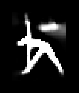
Figure 14: Detecting and sketching the common: (a) The input images. (b) The resulting sketch.

Input images	Output sketch	Input images	Output sketch

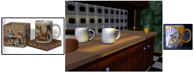
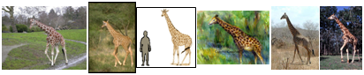
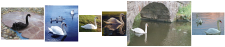
Figure 15: Sample results on ETHZ shapes Ferrari et al. (2006) dataset:  Detection and sketching using only 3 images (left), and using 6 images (right).

Figure 16: Evaluating sketch quality: Mean values of $Quality(S)$ as a function of the number of input images ($K=2,...,10$) randomly sampled from each set of ETHZ shape dataset Ferrari et al. (2006).

Figure 17: Sketching in presence of outliers: We “corrupt” a set of 10 “inlier” with $n$ randomly chosen natural images. Graph shows mean values of $Quality(S)$ as a function of the percent of outlier images in the input set, i.e., $n/(10+n)$.

Figure 18: Detection in new images: We empirically evaluated how well the sketch generated form very few images ($K=2,..10$) performs in detecting the common shape in new images.

Figs. 6,8,11,13,14,15 show qualitative results on various image sets. In all of these examples the number of input images was very small ($3-7$), with large variability in appearance and background clutter. Our algorithm was able to detect and produce a compact representation (a sketch) of the common content.

We further conducted empirical evaluations of the algorithm using ETHZ shape dataset Ferrari et al. (2006). This dataset consists of five object categories with large variability in appearance: Applelogos, Bottles, Giraffes, Mugs and Swans (example images can be seen in Fig. 15). There are around $50$ images in each set, with ground-truth information regarding the location of the object in each image, along with a single hand-drawn ground truth shape for each category. In order to assess the quality of our algorithm (which is currently not scale invariant, although it can handle up to $\pm 20\%$ scale variation, and $\pm 15^{\circ}$ rotations), we scaled the images in each dataset to have roughly the same object size (but we have not rotated the images, nor changed their aspect ratios).

Sketch quality score: Because our sketch $S$ is continuous in the range $\left[-1,\ 1\right]$, we stretch the values of the ground-truth sketch $S_{GT}$ also to this range, and multiply the two sketches pixel-wise. Our sketch quality score is:  $Quality(S)={<S,S_{GT}>}/{(\#\leavevmode\nobreak\ of\leavevmode\nobreak\ pixels)}.$ In places where both sketches agree in their sign (either white regions or black) the pixel-wise product is positive, while in places where the sketches disagree, the product is negative. This produces a sketch quality score with values ranging between $-1$ (lowest quality) to $+1$ (highest quality). Note that even if our sketch displays a perfect shape, its quality will be smaller than $1$, because it is not a perfect binary image. From our experience, sketch quality $\geq 0.8$ are usually excellent-looking sketches.

We first assessed the quality of our algorithm to identify and sketch the common object correctly, as a function of the number of input images $K$ ($K=2,3,..,10$). We randomly sampled $K$ images out of an object category set, applied our detection and sketching algorithm to that subset, and compared the resulting sketch $S$ to the ground-truth $S_{GT}$. We repeated this experiment $15$ times for each $K$, and computed mean sketch quality scores. Fig. 18 displays plots of the mean quality score for the $5$ categories. It can be seen that from relatively few images ($K=3$) we already achieve sketches of good quality, even for challenging sets such as the giraffes (although, with the increased number of example images, its legs tend to disappear from the sketch because of their non-rigid deformations). Examples for sketching results for some of these experiments can be seen in Fig. 15.

We next evaluated the robustness of the sketching component of our algorithm to outliers. Such robustness is important, since the detection algorithm often produces outlier detections (see Fig. 10). We used $10$ “inlier” images which alone generate a good sketch with high sketch quality score. We then added to them $n=1,...,30$ outlier images (cropped at random from natural images). For every such $10+n$ image set we generated a sketch, and compared it to the ground-truth. Each experiment was repeated $15$ times. Fig. 18 displays plots of sketch quality vs. percent of outliers $n/(10+n)$. Our sketching method is relatively robust to outliers, and performs quite well even in presence of $50\%$ outliers (as expected due to the median operation in Eq. (27)).

In addition to sketch quality evaluation we tested the performance of our algorithm in the scenario described in the Introduction: given a very small number of example images, how useful is the output of our automatical detection & sketching algorithm for successfully detecting that object in new images. For $K=2,3,...,10$, we randomly sampled $K$ images out of an object category set, applied our detection & sketching algorithm to that subset, and used the resulting sketch to detect the object in the remaining $50-K$ images of that category set. We consider an object in image $I_{n}$ as “detected” if the location of $maxMatch(S,I_{n})$ (the detected center $c_{n}$ of the object) falls no farther away than 1/4 of the width or height of the bounding-box from the ground-truth center. We repeated each experiment $40$ times and plotted the average detection rates in Fig. 18. For the Apples, Bottles, and Swans we get high detection rates (for as few as $K=3$ example images; a scenario no WSL method can handle to the best of our knowledge). However, our detection rates are not as good in the Giraffe set, since the giraffes undergo strong non-rigid deformations (they sometimes tilt their necks down, and their legs change positions). Our current algorithm cannot handle such strong non-rigid deformations.

Chapter 4 Negative Affinities

Clustering is a fundamental task in unsupervised learning. The focus of this chapter is the Correlation Clustering (CC) functional which combines positive and negative affinities between pairs of data points. In this chapter we provide a theoretical analysis of the CC functional. Our analysis suggests a probabilistic generative interpretation for the functional, and justifies its intrinsic “model-selection” capability. In addition we suggest two new applications that utilize the “model-selection” capability of CC: unsupervised face identification and interactive multi-object segmentation by rough boundary delineation.

The resulting CC energy is arbitrary and is very difficult to approximate. We defer the discussion on our approximate minimization algorithms for the CC energy to chapter 7 in part III, which deals with approximation schemes for arbitrary energies.

12 Introduction

One of the fundamental tasks in unsupervised learning is clustering: grouping data points into coherent clusters. In clustering of data points, two aspects of pair-wise affinities can be measured: (i) Attraction (positive affinities), i.e., how likely are points $i$ and $j$ to be in the same cluster, and (ii) Repulsion (negative affinities), i.e., how likely are points $i$ and $j$ to be in different clusters.

Indeed, new approaches for clustering, recently presented by Yu and Shi (2001) and Bansal et al. (2004), suggest to combine attraction and repulsion information. Normalized cuts was extended by Yu and Shi (2001) to allow for negative affinities. However, the resulting functional provides sub-optimal clustering results in the sense that it may lead to fragmentation of large homogeneous clusters.

The Correlation Clustering functional (CC), proposed by Bansal et al. (2004), tries to maximize the intra-cluster agreement (attraction) and the inter-cluster disagreement (repulsion). Contrary to many clustering objectives, the CC functional has an inherent “model-selection” property allowing to automatically recover the underlying number of clusters (Demaine and Immorlica (2003)).

Sec. 13 focuses on a theoretical probabilistic interpretation of the CC functional. The subsequent sections (Sec. 14 and 15) present two new applications. Both these applications build upon integrating attraction and repulsion information between large number of points, and require the robust recovery of the underlying number of clusters $k$.

This chapter focuses on the CC functional, its properties and derived applications. We defer to chapter 7 our novel approach to CC optimization. Experimental results presented in this chapter were produced using our algorithms, which are described in more detail in chapter 7.

Correlation Clustering (CC) Functional

Let $W\in\mathbb{R}^{n\times n}$ be an affinity matrix combining attraction and repulsion: for $W_{ij}>0$ we say that $i$ and $j$ attract each other with certainty $\left|W_{ij}\right|$, and for $W_{ij}<0$ we say that $i$ and $j$ repel each other with certainty $\left|W_{ij}\right|$. Thus the sign of $W_{ij}$ tells us if the points attract or repel each other and the magnitude of $W_{ij}$ indicates our certainty.

Any $k$-way partition of $n$ points can be written as $U\in\left\{0,1\right\}^{n\times k}$ s.t. $U_{ic}=1$ iff point $i$ belongs to cluster $c$. $\sum_{c}U_{ic}=1\;\forall i$ ensure that every $i$ belongs to exactly one cluster.

The CC functional maximizes the intra-cluster agreement (Bansal et al. (2004)). Given a matrix $W$, an optimal partition $U$ minimizes:

$$\mathcal{E}_{CC}\left(U\right) = -\sum_{ij}W_{ij}\sum_{c}U_{ic}U_{jc}$$

$$s.t. U_{ic}\in\left\{0,1\right\},\;\sum_{c}U_{ic}=1$$

Note that $\sum_{c}U_{ic}U_{jc}$ equals 1 iff $i$ and $j$ belong to the same cluster. For brevity, we will denote $\sum_{c}U_{ic}U_{jc}$ by $\left[UU^{T}\right]_{ij}$ from here on.

13 Probabilistic Interpretation

This section provides a probabilistic interpretation for the CC functional. This interpretation allows us to provide a theoretic justification for the “model selection” property of the CC functional. Moreover, our analysis exposes the underlying implicit prior that this functional assumes.

We consider the following probabilistic generative model for matrix $W$. Let $U$ be the true unobserved partition of $n$ points into clusters. Assume that for some pairs of points $i,j$ we observe their pairwise similarity values $s_{ij}$. These values are random realizations from either a distribution $f^{+}$ or $f^{-}$, depending on whether points $i,j$ are in the same cluster or not. Namely,

$$p\left(s_{ij}=s\left|\left[UU^{T}\right]_{ij}=1\right.\right) = f^{+}\left(s\right)$$

$$p\left(s_{ij}=s\left|\left[UU^{T}\right]_{ij}=0\right.\right) = f^{-}\left(s\right)$$

Assuming independency of the pairs, the likelihood of observing similarities $\left\{s_{ij}\right\}$ given a partition $U$ is then

$$\mathcal{L}\left(\left\{s_{ij}\right\}\left|U\right.\right)=\prod_{ij}f^{+}\left(s_{ij}\right)^{\left[UU^{T}\right]_{ij}}\cdot f^{-}\left(s_{ij}\right)^{\left(1-\left[UU^{T}\right]_{ij}\right)}$$

To infer a partition $U$ using this generative model we look at the posterior distribution:

$$Pr\left(U\left|\left\{s_{ij}\right\}\right.\right)\propto\mathcal{L}\left(\left\{s_{ij}\right\}\left|U\right.\right)\cdot Pr\left(U\right)$$

where $Pr\left(U\right)$ is a prior. Assuming a uniform prior over all partitions, i.e., $Pr\left(U\right)=const$, yields:

$$Pr\left(U\left|\left\{s_{ij}\right\}\right.\right)\propto\prod_{ij}f^{+}\left(s_{ij}\right)^{\left[UU^{T}\right]_{ij}}\cdot f^{-}\left(s_{ij}\right)^{\left(1-\left[UU^{T}\right]_{ij}\right)}$$

Then, the negative logarithm of the posterior is given by

$$-\log Pr\left(U\left|\left\{s_{ij}\right\}\right.\right) = \hat{C}+\sum_{ij}\log f^{+}\left(s_{ij}\right)\left[UU^{T}\right]_{ij}$$

$$+\sum_{ij}\log f^{-}\left(s_{ij}\right)\left(1-\left[UU^{T}\right]_{ij}\right)$$

where $\hat{C}$ is a constant not depending on $U$.

Interpreting the affinities as log odds ratios $W_{ij}=\log\left(\frac{f^{+}\left(s_{ij}\right)}{f^{-}\left(s_{ij}\right)}\right)$, the posterior becomes

$$-\log Pr\left(U\left|\left\{s_{ij}\right\}\right.\right) = C-\sum_{ij}W_{ij}\left[UU^{T}\right]_{ij}$$ (32)

That is, Eq. (32) estimates the log-posterior of a partition $U$. Therefore, a partition $U$ that minimizes Eq. (32) is the MAP (maximum a-posteriori) partition. Since Eq. (4) and Eq. (32) differ only by a constant they share the same minimizer: the MAP partition.

13.1 Recovering $k$ (a.k.a. “model selection”)

We showed that the generative model underlying the CC functional has a single model for all partitions, regardless of $k$. Therefore, optimizing the CC functional one need not select between different generative models to decide on the optimal $k$. Comparing partitions with different $k$ is therefore straight forward and does not require an additional “model complexity” term (such as BIC, MDL, etc.)

As described in the previous section the CC functional assumes a uniform prior over all partitions. This uniform prior on $U$ induces a prior on the number of clusters $k$, i.e., what is the a-priori probability of $U$ having $k$ clusters: $Pr\left(k\right)=Pr\left(U\mbox{ has $k$ clusters}\right)$. We use Stirling numbers of the second kind (Rennie and Dobson (1969)) to compute this induced prior on $k$. Fig 19 shows the non-trivial shape of this induced prior on the number of clusters $k$.

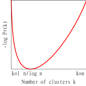
Figure 19: Prior on the number of clusters $k$: Graph shows $-\log Pr\left(k\right)$, for uniformly distributed $U$. The induced prior on $k$ takes a non-trivial shape: it assigns very low probability to the trivial solutions of $k=1$ and $k=n$, while at the same time gives preference to partitions with non-trivial $k$. The mode of this prior is when $U$ has roughly $\frac{n}{\log n}$ clusters.

14 Interactive multi-object segmentation (Patent Pending)

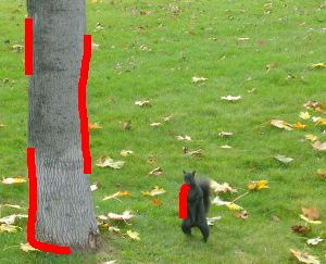
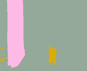
(a) Input image and boundary scribbles (red)	(b) Resulting segmentation

Figure 20: Interactive multi-object segmentation: (a) The user provides only crude and partial indications to the locations of boundaries between the relevant objects in an image (red). (b) The output of our algorithm correctly segments the image into multiple segments. Image was taken from Alpert et al. (2007).

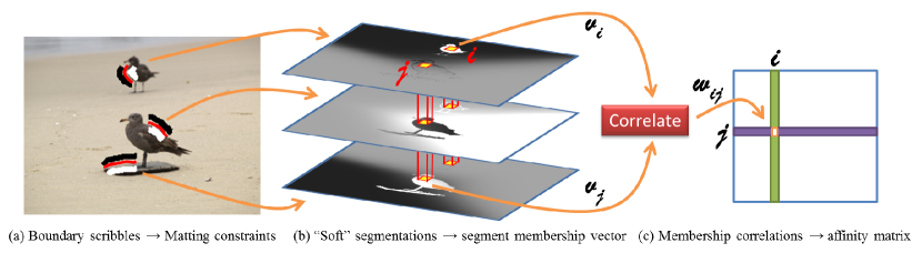
Figure 21: From boundary scribbles to affinity matrix: (a) A boundary scribble is drawn by the user (red), inducing “figure/ground” regions on its opposite sides (black and white regions). (b) For each scribble we use the method of Levin et al. (2008) to generate a soft segmentation of the image into two segments: pixel values in the soft segmentation are in the range $\left[-1,1\right]$. Pixels far away from the scribble are assigned 0 as it is uncertain to what segment they should belong to. Each pixel $i$ is described using a segmentation membership vector $v_{i}$ with an entry corresponding to its assignment at each soft segmentation (red columns). (c) A non-zero entry $w_{ij}$ in the sparse affinity matrix is the correlation between normalized vectors $v_{i}$ and $v_{j}$: $w_{ij}=v_{i}^{T}v_{j}/\left\|v_{i}\right\|\cdot\left\|v_{j}\right\|$. We also add strong repulsion across each scribble.

Negative affinities in image segmentation may come very naturally from boundary information: pixels on the same side of a boundary are likely to be in the same segment (attraction), while pixels on opposite sides of a boundary are likely to be in different segments (repulsion). We use this observation to design a novel approach to interactive multi-object image segmentation. Instead of using $k$ different “strokes” for the different objects (e.g., Santner et al. (2011)), the user applies a single “brush” to indicate parts of the boundaries between the different objects. Using these sparse and incomplete boundary hints we can correctly complete the boundaries and extract the desired number of segments. Although the user does not provide at any stage the number of objects $k$, our method is able to automatically detect the number of segments using only the incomplete boundary cues. Fig. 20 provides an example of our novel interactive multi-object segmentation approach.

Computing affinities: Fig. 21 illustrates how we use sporadic user-provided boundary cues to compute a sparse affinity matrix with both positive and negative entries. Note that this is a modification of the affinity computation presented by Stein et al. (2008): (i) We use the interactive boundary cues to drive the computation, rather than some boundaries computed by unsupervised technique. (ii) We only compute a small fraction of all entries of the matrix, as opposed to the full matrix of Stein et al.(iii) Most importantly, we end up with both positive and negative affinities in contrast to Stein et al. who use only positive affinities.

The sparse affinity matrix $W$ is very large ($\sim 100k\times 100k$). Existing methods for optimizing the correlation clustering functional are unable to handle this size of a matrix. Chapter 7 describes in detail our novel approach to CC optimization that enables us to optimize such large scale problems. We applied our Swap-and-Explore algorithm (Alg. 2, described in 33) to this problem and it provides good looking results with only several minutes of processing per image.

Fig. 22 shows input images and user marked boundary cues used for computing the affinity matrix. Our results are shown at the bottom row.

The new interface allows the user to segment the image into several coherent segments without changing brushes and without explicitly enumerate the number of desired segments to the algorithm.

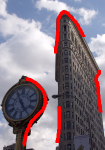
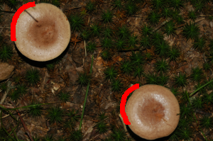
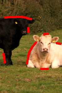
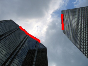
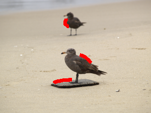
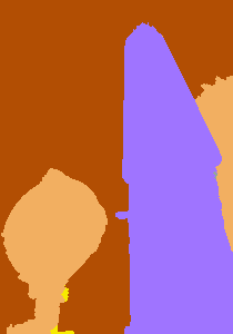
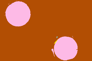
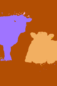
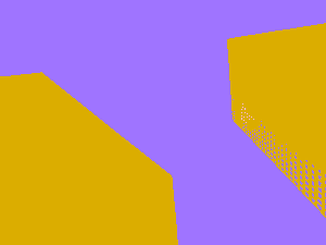
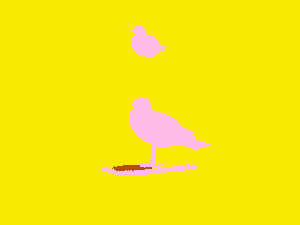
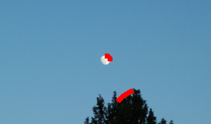
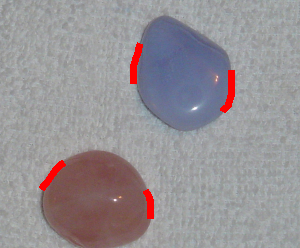
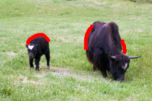
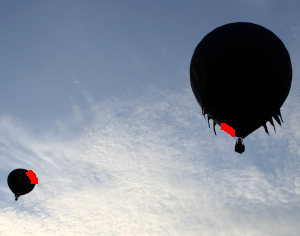
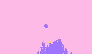
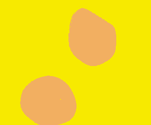
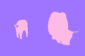
Figure 22: Interactive segmentation results. Input image and user boundary cues (top), our result (bottom). Images were taken from Alpert et al. (2007).

15 Clustering and face identification

This application shows that detecting the underlying number of clusters $k$ can be an important task on its own. Given a collection of face images we expect the different clusters to correspond to different persons. Identifying the different people requires not only high purity of the resulting clusters but more importantly to correctly discover the appropriate number of clusters. This experiment is an extension of existing work on the problem of “same/not-same” learning. Following recent metric learning approach (e.g., Guillaumin et al. (2009, 2010)) we learn a single classifier that assigns a probability to each pair of faces: “how likely is this pair to be of the same person”. Then, using this classifier, we are able to determine the number of persons and cluster the faces of unseen people. That is, given a new set of face images of several unseen people, our clustering approach is able to automatically cluster and identify how many different people are in the new set of face images of never seen before people.

For this experiment we use PUT face dataset Kasinski et al. (2008). The dataset consists of 9971 images of 100 people (roughly 100 images per person). Images were taken in partially controlled illumination conditions over a uniform background. The main sources of face appearance variations are changes in head pose, and facial expression.

We use the same method as Guillaumin et al. (2009) to describe each face. SIFT descriptors are computed at fixed points on the face at multiple scales. We use the annotations provided in the dataset to generate these keypoints. Given a training set of labeled faces $\left\{x_{i},y_{i}\right\}_{i=1}^{N}$ we use a state-of-the-art method by Guillaumin et al. (2010) to learn a Mahalanobis distance $L$ and threshold $b$ such that:

$$Pr\left(y_{i}=y_{j}|x_{i},x_{j};L,b\right)=\sigma\left(b-\left(x_{i}-x_{j}\right)^{T}L^{T}L\left(x_{i}-x_{j}\right)\right)$$

where $\sigma(z)=(1-e^{-z})^{-1}$ is the sigmoid function.

For each experiment we chose $k$ people for test (roughly $100\cdot k$ images), and used the images of the other $100-k$ people for training. The learned distance is then used to compute $p_{ij}$, the probability that faces $i$ and $j$ belong to the same person, for all pairs of face images of the $k$ people in the test set. The affinities are set to $W_{ij}=\log\frac{p_{ij}}{1-p_{ij}}$. We apply our clustering algorithm to search for an optimal partition, and report the identified number of people $k^{\prime}$ and the purity of the resulting clusters. We experimented with $k=15,20,\ldots,35$. For each $k$ we repeated the experiments for several different choices of $k$ different persons.

In these settings all our algorithms, described in Sec. 33, performed roughly the same in terms of recovering $k$ and the purity of the resulting clustering. However, in terms of running time adaptive-label ICM completed the task significantly faster than other methods. We compare Swap-and-Explore (Alg. 2 of Sec. 33) to two different approaches: (i) Connected components: Looking at the matrix of probabilities $p_{ij}$, thresholding it induces $k^{\prime}$ connected components. Each such component should correspond to a different person. At each experiment we tried 10 threshold values and reported the best result. (ii) Spectral gap: Treating the probabilities matrix as a positive affinity matrix we use NCuts Shi and Malik (2000) to cluster the faces. For this method the number of clusters $k^{\prime}$ is determined according to the spectral gap: Let $\lambda_{i}$ be the $i^{th}$ largest eigenvalue of the normalized Laplacian matrix, the number of clusters is then $k^{\prime}=\arg\max_{i}\frac{\lambda_{i}}{\lambda_{i+1}}$.

Fig. 23 shows cluster purity and the number of different persons $k^{\prime}$ identified as a function of the actual number of people $k$ for the different methods. Our method succeeds to identify roughly the correct number of people (dashed black line) for all sizes of test sets, and maintain relatively high purity values.

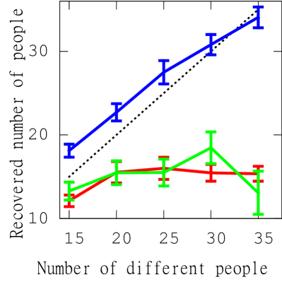
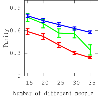
Figure 23: Face identification: Graphs showing our result (Swap), spectral and connected components. Left: recovered number of people ($k^{\prime}$) vs. number of people in the test set. Dashed line shows the true number of people. Right: purity of resulting clusters.

16 Conclusion

This chapter provides a generative probabilistic interpretation for the Correlation Clustering functional, justifying its intrinsic “model selection” capability. Using a generative probabilistic formulation allows for a better understanding of the functional, underlying assumptions it makes, including the prior it imposes on the solution.

Optimizing large scale CC and robustly recovering the underlying number of clusters allows us to propose new applications: interactive multi-label image segmentation and unsupervised face identification.

Chapter 5 3D Shape Reconstruction by Combining Motion and Lighting Cues

In this chapter we consider the problem of reconstructing the 3D shape of a moving object while accounting for the change of intensities due to a change in orientation with respect to the light sources. We assume that both the lighting and motion parameters are given. Two methods are presented. First, for lambertian objects illuminated by a point source we derive a PDE that is quasilinear and implicit in the surface shape. We propose to solve this PDE by continuation (characteristic curves), extending an existing method to allow for large motion. Secondly, we formulate the reconstruction problem as an MRF and solve it using discrete optimization techniques. The latter method works with fairly general reflectance functions and can be applied to sequences of two or more images. It can also incorporate prior information and boundary conditions. We further discuss a method for extracting boundary conditions. We demonstrate the performance of our algorithms by showing reconstructions of smooth shaped objects and comparing these reconstructions to reconstructions with laser scans.

17 Introduction

Moving objects change their appearance as they change their orientation with respect to a light source. Such changes make it difficult to identify corresponding points across images, and as a result complicate the task of motion recovery and subsequently also of 3D reconstruction. Existing approaches to motion analysis largely assume either brightness constancy, or rely on extracting distinctive features. These approaches successfully handle both polygonal shapes and objects with noticeable surface markings, but they are less suitable for handling objects with smooth shapes and gradual albedo variations.

In this paper we propose a framework for reconstructing the shape of such objects that explicitly takes lighting effects into account. Our work is based on the observation that the changes in both the location and intensity of a moving object across images are coupled by its motion. Therefore, these two sources of information can be combined to constrain the matching of points across images, allowing us to achieve a veridical reconstruction. A number of previous studies (see Section 18) used this observation to propose algorithms for shape recovery either in multi-view settings or in restricted settings (single directional light source and small motion, Basri and Frolova (2008)) when only two views are available. In this study we propose a method that can work with two or more images and that can deal with general lighting conditions and fairly large motion.

We consider the case of an object that moves rigidly with respect to the camera and the light source. We assume that the object is lambertian, and that both the lighting conditions and the motion parameters are known. We present two algorithms. First we address the problem of shape reconstruction from two views when lighting is composed of a single directional source, and derive a partial differential equation (PDE) that can be solved to recover the shape of the object using continuation (characteristic curve). We further show how we can derive boundary conditions for this method. This formulation extends the work of Basri and Frolova (2008) to objects undergoing a large motion.

Our second algorithm uses the PDE formulation to construct a cost function on a graph, representing the domain to be reconstructed. The cost function takes the form of a Markov Random Field (MRF). We then use off-the-shelf algorithms to solve for the sought shape. The MRF formulation offers several advantages over previous work. (1) It can work with fairly general reflectance functions. (2) It can be applied to pairs of images as well as to sequences of three or more images. (3) It is more robust to errors than continuation solutions, which can accumulate errors in integration. Finally, (4) prior information can be incorporated; in particular, the method can use boundary conditions, but as we show in our experiments boundary conditions are not essential. Experiments with real smooth objects demonstrate the utility of our formulation.

The paper is divided as follows. Section 18 provides a brief summary of related work. Section 19 defines the reconstruction problem and derives a continuation solution in the case of large motion. Section 20 casts the problem as an MRF optimization and discusses its solution by discrete techniques. Section 21 explains how we compute boundary conditions, and Section 22 shows the results of our experiments.

18 Previous work

The majority of 3D reconstruction techniques use either motion or shading techniques, but rarely combine both cues. Shape from shading Horn and Brooks (1989) and photometric stereo Woodham (1980) utilize shading cues to reconstruct objects from single or multiple images of static objects. Motion is often handled with the assumption of brightness constancy Horn and Schunk (1981); Lucas and Kanade (1981) or by matching sparse feature points (e.g., Crandall et al. (2011)). Some authors proposed to reconstruct static objects by combining shading with stereo cues Cryer et al. (1995); Fua and Leclerc (1995). Note that in a stereo setup lambertian objects retain their intensities across images. Another set of studies seek to generalize the brightness constancy assumption to account for local lighting variations Black et al. (2000); Negahdaripour (1998); Haussecker and Fleet (2001).

Studies that use motion and shading cues simultaneously Carceroni and Kutulakos (2001); Jin et al. (2008); Maki et al. (2002); Mukawa (1990); Simakov et al. (2003); Weber et al. (2004); Zhang et al. (2003); Joshi and Kriegman (2007); Chen et al. (2009); Moses and Shimshoni (2006). typically require a multi-frame setting (typically at least 4 images). These studies also estimate the light source direction along with the shape of the object. An exception is Basri and Frolova (2008), which requires only two images, but assumes small motion. Our work improves over these methods by proposing reconstruction methods that can handle large motion and can work both with image pairs and with larger sequences of images. In addition, our second algorithm allows for general lighting settings, which include point and extended light sources, through the use of spherical harmonic representations (Basri and Jacobs (2003); R.Ramamoorthi and P.Hanrahan (2001)).

19 Problem definition and solution by continuation

We consider a pair of images taken by a stationary camera. The images depict a lambertian object moving rigidly in space and illuminated by constant lighting. Denote these images by $I(x,y)$ and $J(x,y)$. Let ${\bf P}=(x,y,z(x,y))$ be a point on the object’s surface described in the coordinate frame of $I$, and let ${\bf p}$ and ${\bf q}$ denote its projections onto $I$ and $J$. Assuming a weak perspective projection ${\bf p}=(x,y)$, and ${\bf q}=sR{\bf P}+{\bf t}$ in $J$, where the scale $s>0$, rotation $R$ (represented by a $2\times 3$ matrix with orthonormal rows) and translation ${\bf t}\in\Re^{2}$ describe the (known) motion of the object. In general, since the motion is assumed to be known the location of ${\bf q}$ depends on the unknown depth value of ${\bf P}$, $z$. We therefore often emphasize this dependence by writing ${\bf q}(z)$.

Denote the normal to the surface at ${\bf p}$ in $I$ by $\hat{\bf n}\in S^{2}$,

$$\hat{\bf n}=\frac{1}{\sqrt{z_{x}+z_{y}+1}}(-z_{x},-z_{y},1),$$

where $z_{x}=\partial z/\partial x$, $z_{y}=\partial z/\partial y$, and denote the albedo at $p$ by $\rho\in\Re$. Thus, the normal at ${\bf q}(z)$ is given by $R\hat{\bf n}$. We assume that the intensity of ${\bf P}$ in the two images can be expressed as $I({\bf p})=\rho r(\hat{\bf n})$ and $J({\bf q})=\rho r(R\hat{\bf n})$, where $r:S^{2}\rightarrow\Re$, commonly referred to as the reflectance function, is a (known) function of the surface normal. This expression can be used to model a variety of materials. In particular, it can model lambertian objects illuminated by a directional (“point”) source by setting $r(\hat{\bf n})=\max({\bf l}^{T}\hat{\bf n},0)$. Here the direction of the point source is given by ${\bf l}/\|{\bf l}\|$ and its intensity by $\|{\bf l}\|$. Likewise, under more general lighting conditions (that may include multiple point and extended sources) $r(\hat{\bf n})$ can be expressed as an inner product between a vector of coefficients ${\bf b}\in\Re^{d}$ and the spherical harmonic functions evaluated at $\hat{\bf n}$, denoted $Y(\hat{\bf n})\in\Re^{d}$. $d$ is set to either 4 or 9 if respectively the first or second order harmonic approximation is used, see Basri and Jacobs (2003) for details of this model.

Under these assumptions we can eliminate the albedo $\rho$ by taking the ratio between the intensities of corresponding points, namely

$$\frac{J({\bf q}(z))}{I({\bf p})}=\frac{r(R\hat{\bf n})}{r(\hat{\bf n})}.$$ (33)

This PDE captures the relation between the shape of the moving object, its motion and the environment lighting. The shape of the object is captured both implicitly by the correspondence between ${\bf p}$ and ${\bf q}(z)$ (in other words, this equation is implicit in $z$), and explicitly by the surface normal (i.e., the partial derivatives of $z$).

For a lambertian object illuminated by a single directional light source ${\bf l}$ Eq. (33) can be written as follows. Let ${\bf n}=(-z_{x},-z_{y},1)^{T}$ (so that $\hat{\bf n}={\bf n}/\|{\bf n}\|$) then

$$\frac{J({\bf q}(z))}{I({\bf p})}=\frac{{\bf l}^{T}R{\bf n}}{{\bf l}^{T}{\bf n}}.$$ (34)

Note that in this equation the nonlinear term $\|{\bf n}\|$ cancels out. Rearranging this equation we obtain

$${\bf a}^{T}{\bf n}=0,$$ (35)

where ${\bf a}(x,y,z)=J({\bf q}(z)){\bf l}-I({\bf p})R^{T}{\bf l}$. The equation is quasi-linear (i.e., linear in the derivatives $z_{x}$ and $z_{y}$), although implicit in $z$

Basri and Frolova (2008) made this equation explicit in $z$ by using a Taylor approximation for $J({\bf q}(z))$ and used the obtained expression to recover the shape of Lambertian objects illuminated by a single directional source. As their method approximates (33) to first order, it can handle only objects undergoing very small motion. Specifically, assuming $I$ and $J$ are rectified such that their epipolar lines are horizontal, they showed that (33) can be written as an explicit, quasilinear PDE

$$az_{x}+bz_{y}=c,$$ (36)

where

$$\vspace{-2mm}a(x,y,z) = l_{1}(I_{\theta}-zJ_{x})-l_{3}I$$

$$b(x,y,z) = l_{2}(I_{\theta}-zJ_{x})$$

$$c(x,y,z) = l_{3}(I_{\theta}-zJ_{x})+l_{1}I.$$

In this equation $J_{x}=\partial J/\partial x$, $I_{\theta}=(J-I)/\theta$ and $\theta$ denotes the angle of rotation about the vertical axis. They further described a solution to (36) using the method of continuation (characteristic curves) and showed a method to extract Dirichlet boundary conditions along the bounding contour of an object.

Our first contribution is to note that Basri and Frolova’s algorithm can be extended also to handle large motion. This is because (35) is quasi-linear even without the Taylor approximation, and so it too can be solved by the method of continuation. Note that, due to (35), ${\bf a}$ lies on the tangent to the surface $z(x,y)$ at ${\bf p}$. Therefore, any curve $\gamma(t)\subset\Re^{3}$ whose tangent at every $t\in[0,1]$ is given by ${\bf a}(\gamma(t))$ is characteristic to (35), and if $\gamma(0)$ happens to lie on $z(x,y)$ the entire curve will lie on $z(x,y)$. To recover $z(x,y)$ the continuation method traces a family of such curves $\{\gamma(t)\}$ by integrating the vectors ${\bf a}(\gamma(t))$ starting from a 1D set of 3D points given as Dirichlet boundary conditions. Unfortunately, as (35) is implicit in $z$, extracting boundary conditions can be complicated; we suggest a method to do this in Section 21.

Finally, we note that the characteristic curves traced with this procedure are all plane curves that lie in parallel planes. This can be readily seen by noticing that ${\bf a}$ is a linear combination of ${\bf l}$ and $R{\bf l}$, and so ${\bf a}^{T}({\bf l}\times R{\bf l})=0$. in general, unless ${\bf l}$ points in the direction of the axis of rotation (denoted ${\bf u}$) these parallel planes are perpendicular to ${\bf u}$ and are independent of ${\bf l}$. Note however that generally the planes that contain the characteristics do not coincide with the epipolar planes except when the axis of rotation is parallel to the image plane. In the case that ${\bf l}$ coincides with ${\bf u}$, (34) becomes degenerate since its right hand side (substituting ${\bf u}$ for ${\bf l}$) is 1. Consequently, $J({\bf q}(z))=I{\bf p}$, and methods that assume constant brightness can be applied. Figure 24 shows a reconstruction obtained with our suggested method for continuation. A toy model was rendered using point source light and rotated by angle of about $4^{\circ}$. The continuation method was applied with exact boundary condition values.

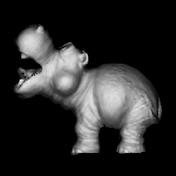
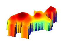
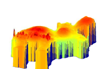
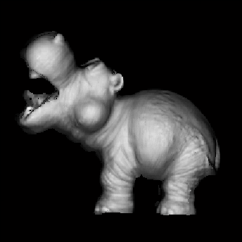
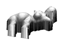
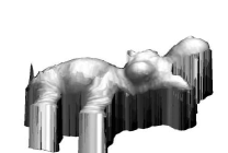
Figure 24: Reconstructions from rendered images of a toy hippo, using continuation. The left column shows the original images (rotation of $4^{\circ}$), the middle column shows the 3D model and the right column shows the reconstructed surface. The top row shows the surface (colormap represents depth values) and the bottom row shows the surface painted with intensity values.

20 Discrete optimization

The continuation method suffers from several shortcomings. First, the method accumulates errors in the integration. Moreover, (33) is quasi-linear when the lighting is composed of a single directional light source, but is non-linear when more realistic lighting models are used. Continuation can in principle be applied also for non-linear equations, but it is then significantly less robust. In addition, the method relies on boundary conditions that are difficult to compute, and at the same time does not allow for the inclusion of other prior information. Finally, it does not provide a way to integrate information from more than two images when more images of the object are available.

To overcome all of these shortcomings we cast the problem as an MRF optimization and solve it using discrete optimization techniques. Our objective is to find a valid surface $z(x,y)$ that satisfies (33). We therefore define a cost function composed of unary and binary terms. Our MRF is defined over a grid overlaid on the first image $I(x,y)$. Each grid point $(x,y)$ is associated with a state vector determining the parameters of the surface element (surfel) observed at that pixel. These parameters include both the depth value and the surface normal, i.e., $(z,z_{x},z_{y})$, of the surfel. Note that such state vectors cannot represent points along the silhouette contour as the derivatives of $z$ at these points diverge. Our cost function combines unary and binary terms over the grid points. The unary term is a function of the residual of (33). Specifically, let

$$T=I({\bf p})r(R\hat{\bf n})-J({\bf q})r(\hat{\bf n}).$$ (37)

We define the unary term as

$$E^{u}_{\bf p}=\exp(\alpha T^{2})-1,$$ (38)

where $\alpha$ is a constant ($\alpha=8$ in our experiments). The binary term is set to prefer integrable surfaces. For ${\bf p}=(x,y)$ we use

$$E^{b}_{\bf p}=(z(x,y)+z_{x}(x,y)-z(x+1,y))^{2}+(z(x,y)+z_{y}(x,y)-z(x,y+1))^{2}.$$ (39)

Our final energy function is given by

$$E=\sum_{{\bf p}\in\Omega_{I}}E^{u}_{\bf p}+\lambda E^{b}_{\bf p},$$ (40)

where $\Omega_{I}$ denotes the silhouette of the object in $I$ and $\lambda$ is constant. (We used values around 0.001.)

In general, when two images are used for reconstruction we need to supply boundary conditions in the form of $z(x,y)$ along a 1D curve $\gamma_{0}$. In Section 21 we describe a technique to estimate the depths near the bounding contours of the object. This procedure provides both the depth values and the normals along a 1D contour in $\Omega_{I}$. Given these boundary conditions we simply modify the unary cost along this contour to vanish in states $(z,z_{x},z_{y})$ that coincide with the depth values and normals predicted by the boundary conditions. As the extraction of boundary conditions can be noisy we then let the optimization modify these depth values. When the optimization is applied to three or more images the additional images further constrain the solution, and so boundary conditions are not necessary.

The binary term is clearly non-submodular. We therefore optimize (40) by a sequence of alpha expansion iterations implemented with the QBPO algorithm Rother et al. (2007). Each iteration solves a binary decision problem in which each variable is allowed to either change its current state to a fixed state $(z^{\alpha},z^{\alpha}_{x},z^{\alpha}_{y})$ or retain its current state. For submodular energies such an iteration is implemented using the st-mincut algorithm Kolmogorov and Zabih (2004); Boykov et al. (2001). The QPBO algorithm extends the st-mincut algorithm to handle negative edge capacities arising in the case of non-submodular pairwise terms. The algorithm constructs a graph with two complimentary vertices for each variable, explicitly representing its two possible binary states. By using a redundant variable representation, the resulting graph can be constructed to have positive capacities in all of its edges, and therefore the st-mincut algorithm can be applied to it. The following rule is used to label the variables at the end of the st-mincut step. Each variable for which its two complimentary vertices fall in different sides of the cut is labeled according to the assignment induced by the cut. Variables for which both complimentary vertices fall in the same side of the cut remain unlabeled. As minimizing non-submodular energies generally is NP-hard, QBPO is not guaranteed to label all the variables after each st-mincut step, and some of the variables may remain unlabeled. These unlabeled variables retain their original label from the previous iteration. This procedure is repeated for every possible choice of a label $(z^{\alpha},z^{\alpha}_{x},z^{\alpha}_{y})$. The entire batch of iterations is then repeated until convergence. The optimization is initialized by setting the initial state $(z,z_{x},z_{y})$ for every point to the state that minimizes the unary term (38).

The discrete optimization solver is followed by a continuous quadratic optimization, in order to relax the quantized labeling (discrete values) of the surface. We solve the following quadratic optimization functional, maintaining the integrability constraint while remaining close to the quantized solution:

$$Ec{z}=\sum_{{\bf p}\in\Omega_{I}}(z(x,y)-\tilde{z}(x,y))^{2}+\mu E^{b}_{\bf p}$$ (41)

where $\tilde{z}(x,y)$ is the solution obtained by the discrete optimization, and$\mu=5$ in our experiments.

Finally, note that this procedure can readily be applied also when the lighting changes between images, by using different reflectance functions for $I$ and $J$ in (37).

21 Boundary conditions

Using the differential relation (33) to reconstruct a shape from two images requires boundary conditions in the form of depth values – one depth value is required along each characteristic curve. This is essential for the continuation method and can be useful for the discrete optimization framework to further constrain the solution. Obtaining depth values can be complicated, as they require finding the correspondence between pixels on a smooth objects. This was bypassed in Basri and Frolova (2008) since under a small motion and with the Taylor expansion (36) becomes explicit in $z$, allowing one to compute the depths at the silhouette contours of the object from the intensities along the contour. Below we describe a method that computes depth values near the silhouette contours when $z$ is implicit.

Denote the object silhouette in $I$ and $J$ respectively by $\Omega_{I}$ and $\Omega_{J}$. We further denote by $\partial_{v}\Omega_{I}$ the portion of the silhouette contour in $I$ that remains visible in $J$ and likewise by $\partial_{v}\Omega_{J}$ the portion of the silhouette contour in $J$ that remains visible in $I$. Let ${\bf P}$ be a rim point in the coordinate frame of $I$ such that its projection onto $I$, denoted ${\bf p}$, lies on $\partial_{v}\Omega_{I}$. Since ${\bf p}$ lies on the bounding contour of $\Omega_{I}$ the surface normal at ${\bf P}$ should be parallel to the normal to the occluding contour at ${\bf p}$, and so it can be derived from the image. Let $\hat{\bf n}({\bf p})=(\cos\beta,\sin\beta,0)^{T}$. Plugging this normal in (33) gives us a scalar for the right hand side, and using the known value $I({\bf p})$ we compute the anticipated intensity at the corresponding point $J({\bf q})$. We can then use this intensity to search along the epipolar line on $J$ to determine ${\bf q}$. This for itself can be complicated, since there may be multiple points in along the epipolar line in $J$ with the anticipated intensity, but in addition we face two problems: (1) the intensity values along the bounding contour are unreliable, and (2) neither the continuation nor our discrete optimization scheme can use normals that are parallel to the image plane.

To overcome these problems we move from ${\bf p}$ one pixel in the direction of the normal into a point ${\bf p}^{\prime}$ inside $\Omega_{I}$. We assume that the surface normal at ${\bf p}^{\prime}$ can be expressed by $\hat{\bf n}({\bf p}^{\prime})=(\cos\beta\cos\psi,\sin\beta\cos\psi,\sin\psi)^{T}$ for some unknown angle $\psi$. Our aim then is to find a point ${\bf q}^{\prime}$ in $J$ along the epipolar line of ${\bf p}^{\prime}$, denoted $e({\bf p}^{\prime}_{i})$, that satisfies (33) with this normal. This equation has two unknowns, the corresponding point ${\bf q}^{\prime}$ in Image $J$ and $\psi$. We therefore regularize the problem by requiring the curve near $\partial_{v}\Omega_{I}$ to be mapped to a continuous curve in $J$.

We define the following optimization function.

$$\min_{\{{\bf q}^{\prime}_{i},\psi_{i}\}}\sum_{{\bf p}_{i}\in\partial_{v}\Omega_{I}}T({\bf p}^{\prime}_{i},{\bf q}^{\prime}_{i},\psi_{i})^{2}+\mu_{1}\|{\bf q}^{\prime}_{i}-{\bf q}_{i}^{0}\|^{2}+\mu_{2}\mathrm{dist}(e({\bf p}^{\prime}_{i}),{\bf q}^{\prime}_{i})^{2}+$$

$$\mu_{3}\|{\bf q}^{\prime}_{i}-{\bf q}_{i-1}^{\prime}\|^{2}+\mu_{4}(\cos\psi_{i}-\cos\psi_{i-1})^{2},$$

where $T(.)$ denotes the residual defined in (37) for a pair of points ${\bf p}^{\prime}_{i}$ and ${\bf q}^{\prime}_{i}$ and normal $\hat{\bf n}({\bf p}^{\prime})$ parameterized by $\psi$, and $\mathrm{dist}(e({\bf p}^{\prime}_{i}),{\bf q}^{\prime}_{i})$ denotes the Euclidean distance between the point ${\bf q}^{\prime}_{i}$ and the epipolar line $e({\bf p}^{\prime}_{i})$. For ${\bf q}_{i}^{0}$ we use the point along $e({\bf p}_{i})$ closes to the boundary (at the same side as ${\bf p}$) that has the intensity anticipated from (33). This heuristic is useful with reasonable rotations. To solve this minimization we substitute for $J({\bf q}^{\prime}_{i})$ in $T({\bf q}^{\prime}_{i},\psi_{i})$ (37) its Taylor expansion around ${\bf q}_{i}^{0}$. The resulting system of equations is non-linear and we solve it by alternate minimization.

We repeat this procedure for $\partial_{v}\Omega_{J}$ to obtain boundary conditions from both sides of the object’s silhouette. Figure 25 shows an example for boundary conditions obtained with our method.

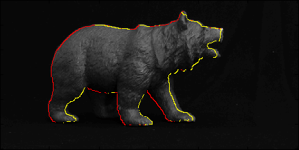
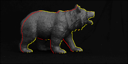
Figure 25: The figure shows boundary conditions computed for two images of a bear toy. The red curve segments depict boundary points ${\bf p}^{\prime}$ in the left image and their selected corresponding points in the right image. The yellow curve segments depict correspondences computed in the opposite direction.

22 Experiments

We tested our algorithm on two sets of real images and compared them to reconstructions with laser scans. Each image is taken with dark background to allow segmentation of the foreground object. In each image we estimated the motion parameters by manually marking points on the image and the 3D mesh object. As the objects are smooth and contain almost no clear surface markings our motion estimates are not perfect. Subsequently, using the mesh we estimated the environment lighting conditions by calculating the 4 coefficients of the first order harmonic representation of the lighting, representing the ambient lighting and a directional source. The obtained motion and lighting parameters were used as input to our software. The figures below show reconstructions obtained with our optimization algorithm (Section 20). We measure the quality of the matches obtained using the RMSE error in pixels. The figures show input images of a bear and elephant toys, reconstructions from pairs of images with and without boundary conditions (Section 21), and reconstructions from multiple images. Our experiments cover a range of rotations between $4^{\circ}$ to about $21^{\circ}$. It can be seen that for the tested our reconstructions achieve low RMSE values. Interestingly, there is no noticeable advantage to using boundary conditions.

23 Conclusion

We described methods for reconstructing the shape of a moving object that accounts for intensities changes due to a change in orientation with respect to the light sources. In particular, we presented a continuation method and a method based on discrete optimization. Our experiments demonstrates the utility of our methods. The setting requires knowledge of the motion and lighting parameters. We plan in the future to seek ways to relax those limiting assumptions.

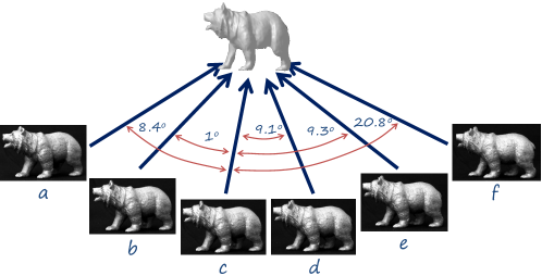
Figure 26: Input images of a bear toy. A laser scan is shown at the center, and relative viewing angles are provided.

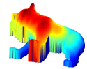
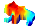
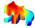
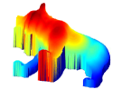
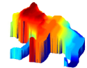
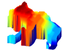
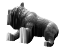
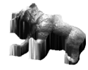
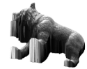
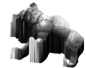
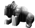
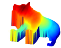
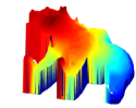
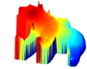
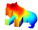
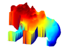
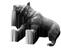
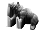
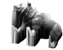
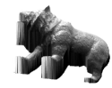
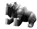
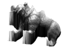
Figure 27: Reconstructions from image pairs. Each box shows from left to right the laser scan, reconstruction with and without boundary conditions. The top row in each box shows the surface (colormap represents depth values) and the bottom row shows the surface painted with intensity values. Reconstructions are shown for images e and g ($9.3^{\circ}$) both achieving RMSE of 1.30 pixels (top left box), images d and f ($10.1^{\circ}$) both achieving RMSE of 1.52 pixels (top right), a and b ($12.1^{\circ}$) achieving 2.24 and 2.20 pixels, and c and e ($16.3^{\circ}$) achieving 3.89 and 3.87.

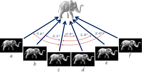
Figure 28: Input images of a elephant toy. A laser scan is shown at the center, and relative viewing angles are provided.

Figure 29: Reconstructions from image pairs. Each box shows from left to right the laser scan, reconstruction with and without boundary conditions. The top row in each box shows the surface (colormap represents depth values) and the bottom row shows the surface painted with intensity values. Reconstructions are shown for images f and b ($7.5^{\circ}$) achieving RMSE 2.14 and 2.12 (top left box) and images b and f ($7.5^{\circ}$) achieving RMSE 1.93 and 1.94 (top right box)

GT (e)	d,e,f	c,d,e,f	c,d,e,f,g
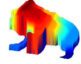
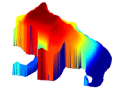
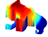
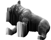
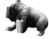
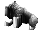
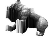
RMSE:	0.88	1.28	1.39
GT (e)	d,e,g	c,d,e,g	d,e,f,g
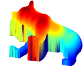
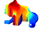
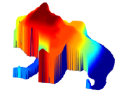
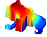
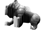
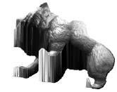
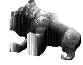
RMSE:	0.88	1.40	0.83

Figure 30: Reconstruction from multiple images. Ground truth is shown at left, image labels at the top and RMSE (over all images) at the bottom.

GT (b)	b,c,f	b,c,d,f	a,b,c,d,e,f
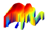
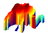
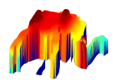
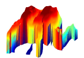
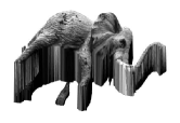
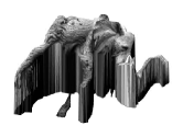
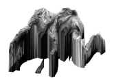
Correspondence error:	1.78	1.44	1.69

Figure 31: Reconstruction from multiple images. Ground truth is shown at left, image labels at the top and RMSE (over all images) at the bottom.

GT (d)	b,c,d,e,f	a,b,c,d,e,f
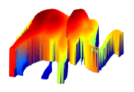
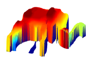
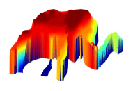
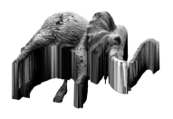
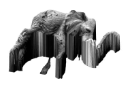
Correspondence error:	0.69	1.30

Figure 32: Reconstruction from multiple images. Ground truth is shown at left, image labels at the top and RMSE (over all images) at the bottom.

Chapter 6 Learning Discrete Energies

This chapter introduces a new formulation for discrete image labeling tasks, the Decision Tree Field (DTF), that combines and generalizes random forests and conditional random fields (CRF) which have been widely used in computer vision. In a typical CRF model the unary potentials are derived from sophisticated random forest or boosting based classifiers, however, the pairwise potentials are assumed to (1) have a simple parametric form with a pre-specified and fixed dependence on the image data, and (2) to be defined on the basis of a small and fixed neighborhood. In contrast, in DTF, local interactions between multiple variables are determined by means of decision trees evaluated on the image data, allowing the interactions to be adapted to the image content. This results in powerful graphical models which are able to represent complex label structure. Our key technical contribution is to show that the DTF model can be trained efficiently and jointly using a convex approximate likelihood function, enabling us to learn over a million free model parameters. We show experimentally that for applications which have a rich and complex label structure, our model outperforms state-of-the-art approaches.

24 Introduction

The last decade has seen the meteoric rise in the use of random field models in computer vision Szeliski et al. (2008). Random fields have been used to model many problems including foreground-background (fg-bg) segmentation Blake et al. (2004); Boykov et al. (2001), semantic segmentation He et al. (2004); Shotton et al. (2007); Winn and Shotton (2006), stereo Boykov et al. (2001), optical flow Baker et al. (2007); Roth and Black (2009); Horn and Schunk (1981), and 3D reconstruction Snow et al. (2000); Vogiatzis et al. (2005). Many of these problems can be cast as an image labeling problem, where we are given an image $\boldsymbol{x}$ and need to predict labels $\boldsymbol{y}$. Random fields provide a way of factorizing the joint distribution $p(\boldsymbol{x},\boldsymbol{y})$ or the posterior distribution $p(\boldsymbol{y}|\boldsymbol{x})$ into a product of local interactions.

In the classic Markov random field (MRF) we obtain the posterior distribution $p(\boldsymbol{y}|\boldsymbol{x})$ by integrating a per-pixel likelihood functions with pairwise consistency potentials ensuring a smooth solution Geman and Geman (1984); Li (1995). One major advance in the field was to make these smoothness cost dependent on the local image structure Boykov et al. (2001), conditioning parts of the model on the input data. In the last decade, these conditional random field (CRF) models Lafferty et al. (2001); Sutton and McCallum (2007); He et al. (2004) have become popular for their improved ability to capture the relationship between labels and the image.

A lot of research effort has been devoted at the development of efficient algorithms for estimating the Maximum a Posteriori (MAP) solution of such models Felzenszwalb and Huttenlocher (2006); Szeliski et al. (2008); Kolmogorov (2006); Komodakis and Tziritas (2007), and the same is true for algorithms for probabilistic inference Wainwright and Jordan (2008); Koller and Friedman (2009). Further, a large number of methods have been proposed to learn the parameters of random field models Anguelov et al. (2005); Kumar et al. (2005); Sutton and McCallum (2007); Szummer et al. (2008); Zhang and Seitz (2005). A number of higher order random field formulations have also been proposed that are able to encode interactions between groups of pixels, and have been shown to produce much better results Kohli et al. (2008); Roth and Black (2009). However, despite these rapid developments, (most) state-of-the-art random field CRF models continue to suffer from the following limitations: (1) they are defined on the basis of a fixed neighborhood structure (except the work of Kolmogorov and Boykov (2005); Roth and Black (2007)), and (2) the potentials are assumed to have a simple parametric form with a pre-specified and fixed dependence on the image data. While it is relatively easy to think of various ways to overcome these limitations, the key research challenge is to suggest a model for which efficient and high-quality training is still tractable.

This paper introduces a new graphical model, the Decision Tree Field (DTF), which overcomes the above-mentioned limitations of existing models. We take a simple yet radical view: every interaction in our model depends on the image, and further, the dependence is non-parametric. It is easy to see that even representing such a model is extremely challenging, since there are numerous ways of defining a mapping between the image and the parameters of a unary or pairwise interaction in the graphical model.

Our model uses decision trees to map the image content to interaction values. Every node of every decision tree in our model is associated with a set of parameters, which are used to define the potential functions in the graphical model. When making predictions on a novel test instance, the leaf node of the decision tree determines the effective weights.

There are a number of important reasons for the choice of decision trees to specify the dependence between potentials and image content. Firstly, decision trees are non-parametric and can represent rich functional relationships if sufficient training data is available. Secondly, the training of decision trees is scalable, both in the training set size and in that the approach can be parallelized; recent advances even allows training on graphics processors Sharp (2008). Since for most computer vision applications it is well known that the key to obtaining high predictive performance is the amount of training data, many recent works use decision trees, or a related variant of it (random Forests Breiman (2001), extremely randomized trees Geurts et al. (2006), semantic texton forest Shotton et al. (2008)). In our context, decision trees give another big advantage: they allow us to efficiently and jointly learn all parameters in the model. We achieve this by using a log-concave pseudo-likelihood objective function, which is known to work well given enough training data because it is a consistent estimator Koller and Friedman (2009).

Our Contributions

(1) To the best of our knowledge, we propose the first graphical model for image labeling problems which allows all potential functions to have an arbitrary dependence on the image data.
(2) We show how the dependence between potential functions and image data can be expressed via decision trees.
(3) We show how the training of the DTF model, which involves learning of a large number of parameters, can be performed efficiently.
(4) We empirically demonstrate that DTFs are superior to existing models such as random forest and common CRFs for applications with complex label interactions and large neighborhood structures.

25 Related Work

There has been relatively little work on learning image-dependent potential functions, i.e. the “conditional part” of a random field. Most algorithms for learning the parameters of a random field try to learn a class-to-class energy table that does not depend on the image content Anguelov et al. (2005); Batra et al. (2008); Nowozin and Lampert (2009); Szummer et al. (2008); Taskar et al. (2005). However, there have been few attempts at learning the parameters of conditional potentials Cho et al. (2010); Prasad et al. (2006); Gould et al. (2009). Recently, Gould et al. Gould et al. (2009) used a multiclass logistic regression classifier on a set of manually selected features, such as the length and orientation of region boundaries to obtain an image-dependent learned model for pairwise interactions. Even more recently, Cho et al. Cho et al. (2010) proposed a model for image restoration whose interactions were dependent on the semantic meaning of the local image content as predicted by a classifier. Unlike our work, all the above-mentioned models either target specific tasks, or assume a particular form for the dependence of the potentials on the image content. Neither of the above-mentioned approaches is able to learn a dependency model with thousands or even millions of parameters which our model can achieve.

Decision trees are popularly used to model unary interactions, e.g., Shotton et al. (2011); but with two exceptions they have not been used for pairwise or higher-order interactions. The first exception is the paper of Glesner and Koller Glesner and Koller (1995), where decision trees are used to model conditional probability tables over many discrete variables in a Bayesian network. The difference to our work is that our decision trees evaluate the given image content, not the state of a random variable, thus requiring no change to the inference procedure used.

The second exception is the “random forest random field” Payet and Todorovic (2010). Despite the similarity in name, the approach is fundamentally different from ours. Instead of defining an explicit model as we do in (43), Payet and Todorovic Payet and Todorovic (2010) define the model distribution implicitly as the equilibrium distribution of a learned Metropolis-Hastings Markov chain. The Metropolis-Hastings ratio is estimated by classification trees. This is a clever idea but comes with a number of limitations, i) at test-time there is no choice between different inference methods but one is bound to using inefficient Markov Chain Monte Carlo (MCMC); in Payet and Todorovic (2010) superpixel graphs of few hundred regions are used and inference takes 30 seconds despite using advanced Swendsen-Wang cuts, and ii) the model remains implicit, such that inspecting the learned interactions as we will do in Section 28.3 is not possible.

In a broader view, our model has a richer representation of complex label structure. Deep architectures, such as Lee et al. (2009) and latent variable CRFs, as in Schnitzspan et al. (2010), have the same goal, but use hidden variables representing the presence of larger entities such as object parts. While these models are successful at representing structure, they are generally difficult to train because their negative log-likelihood function is no longer convex. In contrast, by learning powerful non-parametric conditional interactions we achieve a similar expressive power but retain convexity of the training problem.

26 Model

We now describe the details of our model. Throughout we will refer to $\boldsymbol{x}\in\mathcal{X}$ as a given observed image from the set of all possible images $\mathcal{X}$. Our goal is to infer a discrete labeling $\boldsymbol{y}\in\mathcal{Y}$, where the labeling is per-pixel, i.e., we have $\boldsymbol{y}=(y_{i})_{i\in\mathcal{V}}$, $y_{i}\in\mathcal{L}$, where all variables have the same label set $\mathcal{L}$. We describe the relationship between $\boldsymbol{x}$ and $\boldsymbol{y}$ by means of an energy function $E$ that decomposes into a sum of energy functions $E_{t_{F}}$ over factors $F$, where $F$ defines a subsets of variables. For example, for a pairwise factor it is $|F|=2$. We have

$$E(\boldsymbol{y},\boldsymbol{x},\boldsymbol{w})=\sum_{F\in\mathcal{F}}E_{t_{F}}(y_{F},x_{F},w_{t_{F}}).\vspace{-0.1cm}$$ (42)

By $y_{F}$ we denote the collection $(y_{i})_{i\in F}$, and likewise we write $x_{F}$ to denote the parts of $\boldsymbol{x}$ contained in $F$. While there may be many different subsets in $\mathcal{F}$, we assume they are of few distinct types and denote the type of the factor $F$ by $t_{F}$. The function $E_{t_{F}}$ is the same for all factors of that type, but the variables and image content it acts upon differs. Furthermore, the function is parameterized by means of a weight vector $w_{t_{F}}$ to be discussed below.

A visualization of a small factor graph model is shown in Figure 35. It has three pairwise factor types (red, blue, and green) and two unary factor types (black and turquoise). All factors depend on the image data $\boldsymbol{x}$. Figure 35 shows the “unrolled” factor graph for an image of size 4-by-3 pixels, where the basic model structure is repeated around each pixel $i\in\mathcal{V}$, and pairwise factors which reach outside the image range are omitted. In total we have $|\mathcal{F}|=31$ factors.

The energy function (42) defines a conditional probability distribution $p(\boldsymbol{y}|\boldsymbol{x},\boldsymbol{w})$ as

$$p(\boldsymbol{y}|\boldsymbol{x},\boldsymbol{w})=\frac{1}{Z(\boldsymbol{x},\boldsymbol{w})}\exp(-E(\boldsymbol{y},\boldsymbol{x},\boldsymbol{w})),\vspace{-0.1cm}$$ (43)

where $Z(\boldsymbol{x},\boldsymbol{w})=\sum_{\boldsymbol{y}\in\mathcal{Y}}\exp(-E(\boldsymbol{y},\boldsymbol{x},\boldsymbol{w}))$ is the normalizing constant. So far, our model is in the general form of a conditional random field Lafferty et al. (2001). We now show how to use decision trees for representing $E_{t_{F}}$ in (42).

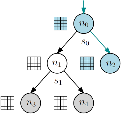
Figure 33: Summation of all energy tables along the path of visited decision nodes (shaded blue).

With each function $E_{t}$ we associate one decision tree. To evaluate $E_{t_{F}}(y_{F},x_{F},w_{t_{F}})$, we start at the root of the tree, and perform a sequence of tests $s$ on the image content $x_{F}$, traversing the tree to the left or right. This process is illustrated in Figure 33. When a leaf node has been reached, we collect the path of traversed nodes from the root node to the leaf node. With each node $q$ of the tree we associate a table of energy values $w_{t_{F}}(q,y_{F})$. Depending on the number of variables $y_{F}$ this energy function acts on, the table can be a vector (unary), a matrix (pairwise), or general $k$-dimensional array (higher order). We sum all the tables along the path taken and compute the energy as

$$E_{t_{F}}(y_{F},x_{F},w_{t_{F}})=\sum_{q\in\textrm{Path}(x_{F})}w_{t_{F}}(q,y_{F}),$$

where $\textrm{Path}(x_{F})$ denotes the set of nodes taken during evaluating the tree. By using one set of weights at each node we can regularize the nodes at the root of the tree to exert a stronger influence, affecting a large number of leaves; at test-time we can precompute the summation along each root-to-leaf path and store the result at each leaf.

To compute the overall energy (42) we evaluate $E_{t_{F}}$ for all factors $F\in\mathcal{F}$. Although the type $t_{F}$ might be the same, the function $E_{t_{F}}$ depends on $x_{F}$ through the evaluation of the decision tree. This allows image-dependent unary, pairwise, and higher-order interactions. The set $\mathcal{F}$ is determined by repeating the same local neighborhood structure for each pixel, as shown in Figures 35 and 35.

In summary, our model consists of a set of factor types. Each factor type contains, (i) the number $k$ of variables it acts on and their relative offsets, (ii) a single decision tree, and (iii) for each node in the decision tree, a table of energies of size $\mathcal{L}^{k}$. Given a new image $\boldsymbol{x}$, for each possible labeling $\boldsymbol{y}$ we can evaluate $E(\boldsymbol{y},\boldsymbol{x},\boldsymbol{w})$ by the above procedure.

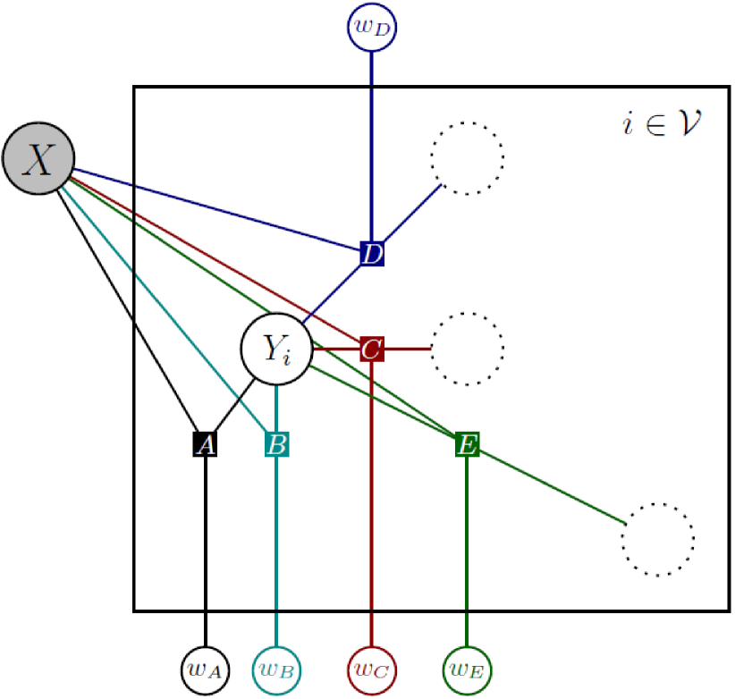
Figure 34: Neighborhood structure around each pixel with five different factor types.

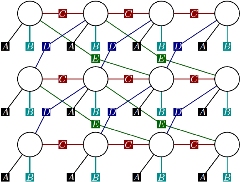
Figure 35: Unrolled factor graph (image size 4-by-3 pixels), dependencies on $\boldsymbol{x}$ and $\boldsymbol{w}$ are not shown.

26.1 Relation to other Models

The proposed DTF generalizes a number of popular existing image labeling methods. If we ignore pairwise and higher-order interactions in (42), then the variables are independent and making predictions for each pixel is the same as evaluating a random forests, as used in e.g. Shotton et al. (2008); Tu and Bai (2010). Interestingly, as we will show in the experiments, even in this setting we still slightly outperform standard random forests since we learn the weights in each decision node instead of using empirical histograms; this novel modification improves predictive performance without any test-time overhead compared to random forests. For pairwise interactions we generalize simple CRFs with contrast-sensitive pairwise potentials such as the popular GrabCut system Rother et al. (2004a) and TextonBoost Shotton et al. (2007). Finally, if for the pairwise interactions we use decision trees of depth one, such that these interactions do not depend on the image content, then our model becomes a classic Markov random field prior Li (1995).

27 Learning Decision Tree Fields

Learning the model involves selecting the neighborhood structure, the decision trees, and the weights stored in the decision nodes. During learning we are given an iid set $\{(\boldsymbol{x}_{m},\boldsymbol{y}^{*}_{m})\}_{m=1,\dots,M}$ of images $\boldsymbol{x}_{m}$ and ground truth labelings $\boldsymbol{y}^{*}_{m}$. Our goal is to estimate the parameters $\boldsymbol{w}$ of our model such as to predict $\boldsymbol{y}^{*}_{m}$ for a given $\boldsymbol{x}_{m}$. For simplifying the derivation of the learning method, we can treat the given set of images as if it would be one large collection of pixels as is done in Sutton and McCallum (2007).

27.1 Maximum Likelihood Learning

For learning the parameters of our model, we need to elaborate on how the parameters $\boldsymbol{w}$ define the energy. One important observation is that for a fixed set of decision trees the energy function (42) can be represented such that it is linear in the parameters $\boldsymbol{w}$. To see this, consider a single $E_{t_{F}}(y_{F},x_{F},w_{t_{F}})$ function and define a binary indicator function

$$B_{t_{F}}(q,z;y_{F},x_{F})=\left\{\begin{array}[]{cl}1&\textrm{if $n\in\textrm{Path}(x_{F})$ and $z=y_{F}$},\\ 0&\textrm{otherwise.}\end{array}\right.$$

Then, we can write the energy $E_{t_{F}}(y_{F},x_{F},w_{t_{F}})$ equivalently as a function linear in $w_{t_{F}}$,

$$\sum_{n\in\textrm{Tree}(t_{F})}\sum_{z\in\mathcal{Y}_{F}}w_{t_{F}}(q,z)B_{t_{F}}(q,z;y_{F},x_{F}).\vspace{-0.1cm}$$ (44)

The use of decision trees allows us to represent non-linear functions on $\boldsymbol{x}$. Although non-linear in $\boldsymbol{x}$, by the representation (44) we can parameterize this function linearly in $w_{t_{F}}$. Then, from (44) we see that the gradient has a simple form, $\nabla_{w_{t_{F}}(q,z)}E_{t_{F}}(y_{F},x_{F},w_{t_{F}})=B_{t_{F}}(q,z;y_{F},x_{F})$.

Because (42) is linear in $\boldsymbol{w}$, the log-likelihood of (43) is a concave and differentiable function in $\boldsymbol{w}$ (Koller and Friedman, 2009, Corollary 20.2). This means that if computing $Z(\boldsymbol{x},\boldsymbol{w})$ and the marginal distributions $p(y_{F}|\boldsymbol{x},\boldsymbol{w})$ for all $F\in\mathcal{F}$ would be tractable, then learning the parameters by maximum likelihood becomes a convex optimization problem.

We now show how to use efficient approximate likelihood methods to learn all parameters associated to the decision trees from training data. For now we assume we are given a fixed set of factor types, including decision trees, but have to learn the weights/energies associated to the nodes of the trees. We will discuss how to learn trees later.

27.2 Pseudolikelihood

The pseudolikelihood Besag (1977) defines a surrogate likelihood function that is maximized. In contrast to the true likelihood function computing the pseudolikelihood is tractable and very efficient. The pseudolikelihood is derived from the per-variable conditional distributions $p(y_{i}|y^{*}_{\mathcal{V}\setminus\{i\}},\boldsymbol{x},\boldsymbol{w})$. By defining $\ell_{i}(\boldsymbol{w})=-\log p(y_{i}|y^{*}_{\mathcal{V}\setminus\{i\}},\boldsymbol{x},\boldsymbol{w})$ we can write the regularized negative log-pseudolikelihood $\ell_{npl}(\boldsymbol{w})$ as the average $\ell_{i}$ over all pixels,

$$\ell_{npl}(\boldsymbol{w})=\frac{1}{|\mathcal{V}|}\sum_{i\in\mathcal{V}}\ell_{i}(\boldsymbol{w})-\sum_{t}\log p_{t}(w_{t}),\vspace{-0.1cm}$$ (45)

where $p_{t}(w_{t})$ is a prior distribution over $w_{t}$ used to regularize the weights. We will use multivariate Normal distributions $\mathcal{N}(0,\sigma_{t}I)$, so that $-\log p_{t}(w_{t})$ is of the form $\frac{1}{2\sigma_{t}^{2}}\|w_{t}\|^{2}+C_{t}(\sigma_{t})$ and the constant $C_{t}(\sigma_{t})$ can be omitted during optimization because it does not depend on $\boldsymbol{w}$. For each factor type $t$ the prior hyperparameter $\sigma_{t}>0$ controls the overall influence of the factor and we need to select a suitable value by means of a model selection procedure such as cross validation.

Function (45) is convex, differentiable, and tractably computable. For optimizing (45) we use the L-BFGS numerical optimization method Zhu et al. (1997). To use L-BFGS we need to iteratively compute $\ell_{i}(\boldsymbol{w})$ and the gradient $\nabla_{w_{t}}\ell_{i}(\boldsymbol{w})$. The computation of $\ell_{i}(\boldsymbol{w})$ and $\nabla_{w_{t}}\ell_{i}(\boldsymbol{w})$ is straightforward

$$\ell_{i}\left(\boldsymbol{w}\right) = \sum_{F\in M(i)}E_{F}\left(y^{*}_{F},\boldsymbol{x},w_{t_{F}}\right)$$ (46)

$$+\log\sum_{y_{i}\in\mathcal{Y}_{i}}\exp\left(-\!\!\sum_{F\in M(i)}\!\!E_{F}\left(y_{i},y^{*}_{\mathcal{V}\setminus\{i\}},\boldsymbol{x},w_{t_{F}}\right)\right)$$

$$\nabla_{w_{t}}\ell_{i}(\boldsymbol{w}) = \sum_{F\in M_{t}(i)}\!\!\!\nabla_{w_{t}}E_{F}\left(\boldsymbol{y}^{*},\boldsymbol{x},w_{t}\right)$$ (47)

$$-\mathbb{E}_{y_{i}\sim p\left(y_{i}\left|y^{*}_{\mathcal{V}\setminus\{i\}},\boldsymbol{x},\boldsymbol{w}\right.\right)}\left[\sum_{F\in M_{t}(i)}\!\!\nabla_{w_{t}}E_{F}\left(y_{i},y^{*}_{\mathcal{V}\setminus\{i\}},\boldsymbol{x},w_{t}\right)\right]$$

where we use $M(i)$ to denote the subset of $\mathcal{F}$ that involves variable $y_{i}$, and $M_{t}(i)$ likewise but restricted to factors of matching type, i.e., $M_{t}(i)=\{F\in M(i):t_{F}=t\}$. By summing (46) and (47) over all pixels in all images, we obtain the objective and its gradient, respectively. When initializing the weights to zero we have approximately $\|\nabla_{\boldsymbol{w}}\ell_{npl}(\boldsymbol{w})\|\approx 1$. During optimization we stop when $\|\nabla_{\boldsymbol{w}}\ell_{npl}(\boldsymbol{w})\|\leq 10^{-4}$, which is the case after around 100-250 L-BFGS iterations, even for models with over a million parameters.

27.3 Learning the Tree Structure

Ideally, we would like to learn the neighborhood structure and decision trees jointly with their weights using a single objective function. However, whereas the weights are continuous, the set of decision trees is a large combinatorial set. We therefore propose to use a simple two-step heuristic to determine the decision tree structure: we learn the classification tree using the training samples and the information gain splitting criterion. This greedy tree construction is popular and known to work well on image labeling problems Shotton et al. (2008). The key parameters are the maximum depth of the tree, the minimum number of samples required to keep growing the tree, and the type and number of split features used. As these settings differ from application to application, we describe them in the experimental section. Unlike in a normal classification tree, we store weights at every decision node and initialize them to zero, instead of storing histograms over classes at the leaf nodes only.

The above procedure is easily understood for unary interactions, but now show that it can be extended in a straightforward manner to learn decision trees for pairwise factors as well. To this end, if we have a pairwise factor we consider the product set $\mathcal{L}\times\mathcal{L}$ of labels and treat each label pair $(l_{1},l_{2})\in\mathcal{L}\times\mathcal{L}$ as a single class. Each training pair of labels becomes a single class in the product set. Given a set of such training instances we learn a classification tree over $|\mathcal{L}|^{2}$ classes using the information gain criterion. Instead of storing class histograms we now store weight tables with one entry per element in $\mathcal{L}\times\mathcal{L}$. The procedure extends to higher-order factors in a straightforward way.

Once the trees are obtained, we set all their weights to zero and optimize (45). During optimization the interaction between different decision trees is taken into account. This is important because the tree structures are determined independently and if we were to optimize their weight independently as well, then we would suffer from overcounting labels during training. The same overcounting problem would occur if we would want to use the class histograms at the leaf nodes directly, for example by taking the negative log-probability as an energy.

27.4 Complexity of Training

The complexity to compute the overall objective (45) and its gradient is $O(|\mathcal{V}|\cdot|\mathcal{L}|\cdot N)$, where $\mathcal{V}$ is the set of pixels in the training set, $\mathcal{L}$ is the label set, and $N$ is the number of factors in the neighborhood structure. Note that this is linear in all quantities, and independent of the order of the factors. This is possible only because of the pseudolikelihood approximation. Moreover, it is even more efficient than performing a single sweep of message passing in loopy belief propagation, which has complexity $O(|\mathcal{V}|\cdot|\mathcal{L}|^{k}\cdot N)$ for factors of order $k\geq 2$.

27.5 Making Training Efficient

Training a graphical model on millions of pixels is computationally challenging. We have two principled methods to make training efficient.

First, observe that our training procedure parallelizes in every step: we train the classification trees in parallel Sharp (2008). Likewise, evaluating (45) and its gradient is a large summation of independent terms, which we again compute in parallel with no communication overhead.

The second observation is that every step in our training procedure can be carried out on a subsampled training set. For classification trees we can process a subset of pixels, as in Shotton et al. (2008). Less obvious, we can do the same thing when optimizing our objective (45). The first term in equation (45) takes the form of an empirical expectation $\mathbb{E}_{i\sim\mathcal{U}(\mathcal{V})}[\ell_{i}(\boldsymbol{w})]$ that can be approximated both deterministically or by means of stochastic approximation. We use a deterministic approximation by selecting a fixed subset $\mathcal{V}^{\prime}\subset\mathcal{V}$ and evaluating $\ell^{\prime}_{npl}(\boldsymbol{w})=\frac{1}{|\mathcal{V}^{\prime}|}\sum_{i\in\mathcal{V}^{\prime}}\ell_{i}(\boldsymbol{w})-\sum_{t}\log p_{t}(w_{t})$. We select $\mathcal{V}^{\prime}$ to be large enough so this computation remains efficient; typically $|\mathcal{V}^{\prime}|$ has a few million elements.

27.6 Inference

We use different inference methods during test-time. For making maximum posterior marginal predictions (MPM) we use an efficient Gibbs sampler. Because the Gibbs sampling updates use the same quantities as used for computing (46) we do not have to unroll the graph. For obtaining approximate MAP predictions, we use the Gibbs sampler with simulated annealing (SA), again exploiting the model structure. Both the Gibbs sampler and the SA minimization is explained in the supplementary materials. To have a baseline comparison, we also minimize (42) using tree-reweighted message passing (TRW) by unrolling the factor graph and using the implementation of Kolmogorov (2006).

28 Experiments

We considered a broad range of applications and report experiments for three data sets. One more experiment is reported in the supplementary materials. The aim is to show that the DTF enables improved performance in challenging tasks, where a large number of interactions and parameters need to be considered and these cannot be manually tuned. Moreover, we show that conditional pairwise interactions better represent the data and lead to improved performance. As the three datasets are quite diverse, they also show the broad applicability of our system.

28.1 Conditional Interactions: Snake Dataset

Figure 36: Input (left), labeling (right).

In this experiment we construct a task that has only very weak local evidence for any particular label and structural information needs to be propagated at test-time in order to make correct predictions. Moreover, this structure is not given but needs to be learned from training data. Consider Figure 36 to the right, illustrating the task. A “snake” shown on the input image is a sequence of adjacent pixels, and the color in the input image encodes the direction of the next pixel: red means “go north”, yellow means “go east”, blue means “go west”, and green means “go south”. Once a background pixel is reached, the snake ends. Each snake is ten pixels long, and each pixel is assigned its own label, starting from the head (black) to the tail (white). Knowing about these rules, the labeling (Figure 36, right) can be perfectly reconstructed. Here, however, these rules need to be learned from training instances. Of course, in a real system the unary interactions typically provide strong cues Shotton et al. (2007); Batra et al. (2008), but we believe that the task distills the limitations of noisy unary interactions: in this task, for making perfect predictions, the unary would need to learn about all possible snakes of length ten, of which there are clearly too many.

We use a standard 4-neighborhood for both the MRF and the DTF models. The unary decision trees are allowed to look at every pixel in the input image, and therefore could remember the entire training image. For experimental details, please see the supplementary materials. We use a training set of 200 images, and a test set of 100 images.

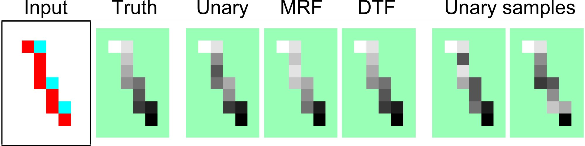
Figure 37: Predictions on a novel test instance.

	RF	Unary	MRF	DTF
Accuracy	90.3	90.9	91.9	99.4
Accuracy (tail)	100	100	100	100
Accuracy (mid)	28	28	38	95

Table 4: Test set accuracies for the snake data set.

The results obtained are shown in Table 4 and Figure 37. Here random forests (RF), trained unary potentials (Unary), and the learned Markov random field (MRF) perform equally well, at around 91%. Upon examining this performance further, we discovered that while the head and tail labels are labeled with perfect accuracy, towards the middle segments of the snakes the labeling error is highest, see Table 4. This is plausible, as for these labels the local evidence is weakest. When using conditional pairwise interactions the performance improves to an almost perfect 99.4%. This again makes sense because the pairwise conditional interactions are allowed to peek at the color-codes at their neighbors for determining the directionality of the snake.

The predictions are illustrated for a single test instance in Figure 37. We see that only the DTF makes a perfect prediction. To show the uncertainty of the unary model, we visualize two samples from the model.

28.2 Learning Calligraphy: Chinese Characters

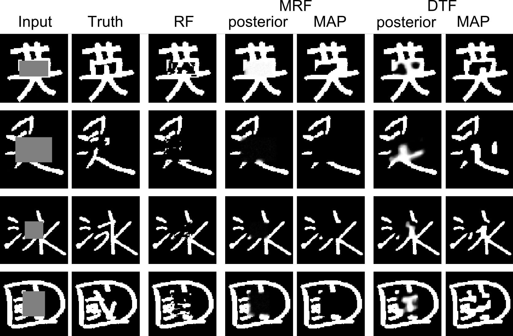
Figure 38: Test set predictions for the large occlusion case.

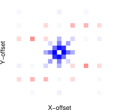
Figure 39: Pairwise associativity strength. Please see text.

In the previous experiment we have used a standard 4-connected neighborhood structure. In this experiment we show that by using larger conditional neighborhoods we are able to represent shape. We use the KAIST Hanja2 database of handwritten Chinese characters. We occlude each character by grey box centered on the image, but with random width and height. For more details, please see the supplementary materials. This is shown in the leftmost column of Figure 38. We consider two datasets, one where we have a “small occlusion” and one with a “large occlusion” box. Note that most characters in the test set have never been observed in the training set, but a model that has learned about shape structure of Chinese characters can still find plausible completions of the input image. To this end we use one unary factor with a decision tree of depth 15. Additionally, we use a dense pairwise neighborhood structure of 8-connected neighbors at one and two pixels distance, plus a sparse set of 27 neighbors at $\{(-9,0),(-9,3),(-9,6),(-9,9),(-6,0),\dots,(9,9)\}$. Therefore, each variable has $2\cdot(24+4+4)=64$ neighboring variables in the model. For the pairwise decision trees we use trees of depth one (MRF), or six (DTF).

The results for the large occlusion task are shown in Figure 38. Qualitatively, they show the difference between a rich connectivity structure and conditional interactions. Observe, for example, that the MRF essentially performs only a smoothing of the results while respecting local stroke-width constraints, as apparent from the MRF MAP prediction in the first row of Figure 38. In contrast, the DTF predictions hallucinate meaningful structure that may be quite different from the ground truth but bears similarity to Chinese characters. Note that we achieve this rich structure without the use of any latent variables. Because this task is an inpainting task, the quantitative assessment is more difficult since the task is truly ambiguous. We therefore report accuracies only for the small-occlusion case, where a reasonable reconstruction of the ground truth seems more feasible. We measure the per-pixel accuracy in the occluded area on the test set. For the random forest baseline we obtain $67.74\%$. The MRF with dense neighborhood improves this to $75.18\%$ and the DTF obtains $76.01\%$.

As an example of what structure the model is able to learn, consider the visualization of the MRF pairwise interactions shown in Figure 39. The figure shows for each pairwise interaction the sum of learned diagonal energies minus the sum of cross-diagonal entries. If this value is negative (shown in blue) the interaction is encouraging the pixels to take the same value. Red marks interactions that encourage pixels to take different values. The plot shows that there is a strong local smoothing term, but interestingly it is not symmetric. This can be explained by the fact that horizontal strokes in Chinese characters are typically slanted slightly upwards Chen (2011). Note that we discovered these regularities automatically from the training data.

28.3 Accurate body-part detection

We consider the task of body part classification from depth images, as recently proposed in Shotton et al. (2011). Given a 2D depth image, and a foreground mask, the task is to label each pixel as belonging to one of 31 different body parts, as shown in Figure 40.

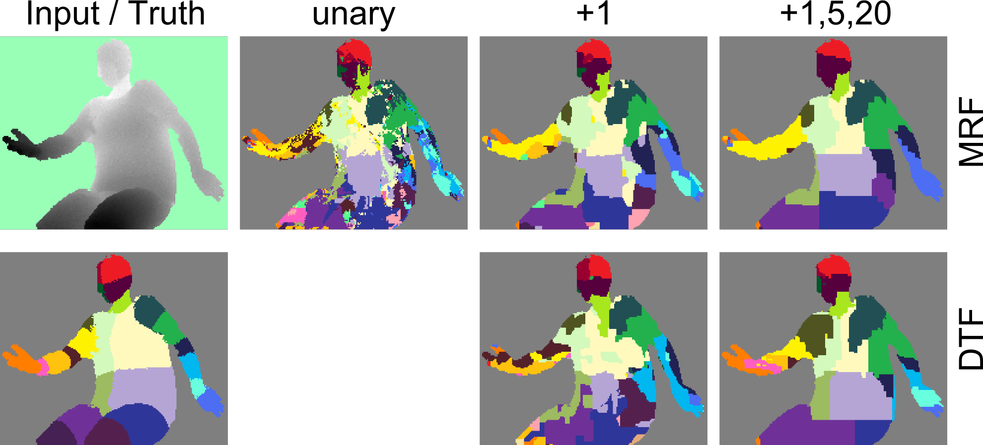
Figure 40: Test recognition results. MRF (top) and DTF (bottom).

Despite the variations in pose and body sizes Shotton et al. (2011) obtains high-quality recognition results by evaluating a random forest for each pixel, testing local and global depth disparities. In this task, the label set has a large amount of structure, but it is not clear that a sufficiently complex unary classifier, when given the image, cannot implicitly represent this structure reasonably well. Here we show that by adding pairwise interactions we in fact improve the recognition accuracy. Moreover, once we make the interactions conditional, accuracy improves even further.

The experimental setup is as follows. We use a subset of the data used in Shotton et al. (2011): 30 depth images for training, and 150 images for testing. We train 4 unary decision trees for all models. For the pairwise models, we use the following neighborhood sizes, (i) “+1” for adding a 4-neighborhood one pixel away, (ii) “+5” for an 8-neighborhood five pixels away, and (iii) “+20” when adding an 8-neighborhood twenty pixels away. In the “+1,5,20” configuration, each variable has 4+8+8=20 neighbors. For each of the pairwise interactions we train two trees of depth six. A more detailed description of the exact experimental setup can be found in the supplementary materials. We measure the results using the same mean per-class accuracy score as used in Shotton et al. (2011).

The results for 30 training images are shown in Table 5 and one instance is shown in Figure 40. Even without adding pairwise interactions, our learned unary weights already outperform the random forest classifier Shotton et al. (2011). When adding more interactions (+1, +1,20, +1,5,20), the performance increases because dense pairwise interactions can represent implicit size preferences for the body parts. Likewise, when adding conditionality (MRF to DTF), the performance improves. The best performing model is our DTF with large structure (+1,5,20) and almost 1.5 million free parameters. It is trained in only 22 minutes and achieves 27.35% mean per-class accuracy. For the same setup of 30 images, the original work Shotton et al. (2011) reports a mean per class accuracy of 14.8%, while achieving an impressive 56.6% when scaling to 900k training images, trained for one day on a 1000 core cluster.

An example of a learned pairwise interaction is shown in Figure 41, demonstrating that the improved performance of the DTF can be directly attributed to the more powerful interactions that are allowed to take the image into account. We report more results in the supplementary materials.

Model	Measure	Shotton et al. (2011)	unary	+1	+1,20	+1,5,20
MRF	avg-acc	14.8	21.36	21.96	23.64	24.05
	runtime	1m	3m18	3m38	10m	10m
	weights	-	176k	178k	183k	187k
DTF	avg-acc	-	-	23.71	25.72	27.35
	runtime	-	-	5m16	17m	22m
	weights	-	-	438k	951k	1.47M

Table 5: Body-part recognition results: mean per-class accuracy, training time on a single 8-core machine, and number of model parameters.

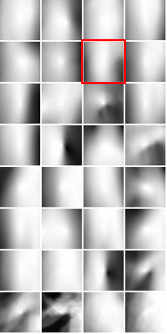
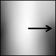
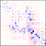
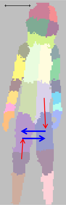
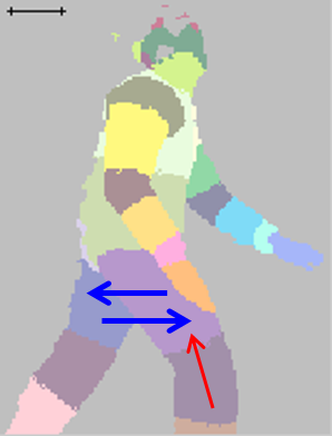
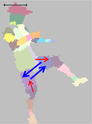
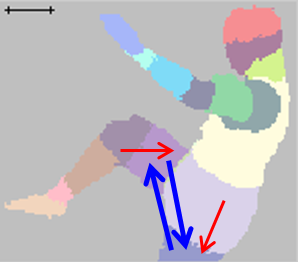
Figure 41: Learned horizontal interactions: The left figure shows the average depth-normalized silhouette reaching one of the 32 leaf nodes in the learned decision tree. We select one leaf (marked red, enlarged) and show the corresponding effective $32\times 32$ weight matrix obtained by summing the learned weights along the path from the root to leaf node. The conditional interaction can be understood by visualizing the most attractive (blue) and most repulsive (red) elements in the matrix. We superimpose arrows for the two most attractive and repulsive interactions on test images (right). The first and second pose exemplify how left and right upper parts of the legs can appear 20 pix to the right of each other in a way that matches the pattern of the leaf. While a configuration like shown in the third and fourth pose is plausible, it does not fit the leaf pattern and thus the interaction is not active.

29 Conclusion

We have introduced Decision Tree Fields as flexible and accurate models for image labeling tasks. This accuracy is achieved by being able to represent complex image-dependent structure between labels. Most importantly, this expressiveness is achieved without the use of latent variables and therefore we can learn the parameters of our model efficiently by minimizing a convex function.

Part III Approximate Optimization

In the previous part several different applications in the domain of computer vision were presented to demonstrate the enhanced descriptive power gained by considering arbitrary energies. However, this gain comes with a price tag: existing optimization algorithms no longer provide good approximations in practice. This part of my work addresses this issue. It concentrates around the second axis of this thesis, which focuses on practical methods and approaches for approximating the minimization of challenging arbitrary discrete energies.

In particular, Chapter 7 proposes a discrete optimization approach to the correlation clustering functional presented in Chapters 3 and 4. This approach scales gracefully with the number of variables, better than existing approaches (Vitaladevuni and Basri (2010)). In fact, we show that our discrete approach to the CC optimization can handle energies defined over hundreds of thousands of variables, as arise in e.g., image segmentation (Sec. 14). This is by far more variables than any other existing method can handle.

Chapter 8 concludes this part with a more general perspective on discrete optimization. This new perspective is inspired by multiscale approaches and suggests to cope with the NP-hardness of discrete optimization using the multiscale landscape of the energy function. Defining and observing this multiscale landscape of the energy, I propose methods to explore and exploit it to derive coarse-to-fine optimization framework. This new perspective gives rise to a unified multiscale framework for discrete optimization. The proposed multiscale approach is applicable to a diversity of discrete energies, both smoothness-encouraging as well as arbitrary, contrast-enhancing functions.

Chapter 7 Correlation Clustering Optimization

The focus of this chapter is the optimization of the Correlation Clustering functional which combines positive and negative affinities between the data points. The main contribution of this chapter are new optimization algorithms which can cope with large scale problems ($>100K$ variables) that are infeasible using existing methods. We draw an analogy between optimizing this functional and the well known Potts energy minimization. This analogy allows us to suggest several new optimization algorithms, which exploit the intrinsic “model-selection” capability of the functional to automatically recover the underlying number of clusters. We compare our algorithms to existing methods on both synthetic and real data.

30 Introduction

Optimizing CC is tightly related to many graph partitioning formulations (Nowozin and Jegelka (2009)), however it is known to be NP-hard (Bansal et al. (2004)). Existing methods derive convex continuous relaxations to approximately optimize the CC functional. However, these algorithms do not scale beyond a few thousands of variables. See for example, the works of Nowozin and Jegelka (2009); Bagon et al. (2010); Vitaladevuni and Basri (2010); Glasner et al. (2011).

This work suggests a new perspective on the CC functional, showing its analogy to the known Potts model. This new perspective allows us to leverage on recent advances in discrete optimization to propose new CC optimization algorithms. We show that our algorithms scale to large number of variables ($>100K$), and in fact can tackle tasks that were infeasible in the past, e.g., applying CC to pixel-level image segmentation. In addition, we provide a rigorous statistical interpretation for the CC functional and justify its intrinsic model selection capability. Our algorithms exploit this “model selection” property to automatically recover the underlying number of clusters $k$.

31 CC Optimization: Continuous Perspective

Optimizing the correlation clustering functional (Eq. (4)) is NP-hard (Bansal et al. (2004)). Instead of solving directly for a partition $U$, existing methods optimize indirectly for the binary adjacency matrix $X=UU^{T}$, i.e., $X_{ij}=1$ iff $i$ and $j$ belong to the same cluster. By introducing the binary adjacency matrix the quadratic objective (w.r.t. $U$): $-\sum_{ij}W_{ij}\left[UU^{T}\right]_{ij}$ becomes linear (w.r.t. $X$): $-\sum_{ij}W_{ij}X_{ij}$. The connected components of $X$, after proper rounding, are the resulting clusters, and the number of clusters $k$ naturally emerges. Indirect optimization methods must ascertain that the feasible set consists only of “decomposable” $X$: $X=UU^{T}$. This may be achieved either by posing semi-definite constraints on $X$ (Vitaladevuni and Basri (2010)), or by introducing large number of linear inequalities (Demaine and Immorlica (2003); Vitaladevuni and Basri (2010)). These methods take a continuous and convex relaxation approach to approximate the resulting functional. This approach allows for nice theoretical properties due to the convex optimization at the cost of a very restricted scalability.

Solving for $X$ requires $\sim n^{2}$ variables instead of only $\sim n$ when solving directly for $U$. Therefore, these methods scale poorly with the number of variables $n$, and in fact, they cannot handle more than a few hundreds of variables. In summary, these methods suffer from two drawbacks: (i) recovering $U$ from $X$ is highly susceptible to noise and more importantly (ii) it is infeasible to solve large scale problems by these methods.

32 Our New Perspective on CC

Existing methods view the CC optimization in the context of convex relaxation and build upon methods and approaches that are common practice in this field of continuous optimization. We propose an alternative perspective to the CC optimization: viewing it as a discrete energy minimization. This new perspective allows us to build upon recent advances in discrete optimization and propose efficient and direct CC optimization algorithms. More importantly, the resulting algorithms solve directly for $U$, and thus scales significantly better with the number of variables.

We now show how to cast the CC functional of Eq.(4) as a discrete pair-wise conditional random field (CRF) energy. For ease of notation, we describe a partition $U$ using a labeling vector $L\in\left\{1,2\ldots\right\}^{n}$: $l_{i}=c$ iff $U_{ic}=1$. A general form of pair-wise CRF energy is $E\left(L\right)=\sum_{i}E_{i}\left(l_{i}\right)+\sum_{ij}E_{ij}\left(l_{i},l_{j}\right)$ (Boykov et al. (2001)). Discarding the unary term ($\sum_{i}E_{i}\left(l_{i}\right)$), and taking the pair-wise term to be $W_{ij}$ if $l_{i}\neq l_{j}$ we can re-write the CC functional as a CRF energy:

$$\mathcal{E}_{CC}\left(L\right)=\sum_{ij}W_{ij}\cdot\mathbbm{1}_{\left[l_{i}\neq l_{j}\right]}$$ (48)

This is a Potts model. Optimizing the CC functional can now be interpreted as searching for a MAP assignment for the energy (48).

The resulting Potts energy has three unique characteristics, each posing a challenge to the optimization process:
(i) Non-submodular: The energy is non-submodular. The notion of submodularity is the discrete analogue of convexity from continuous optimization (Lovász (1983)). Optimizing a non-submodular energy is NP-hard, even for the binary case (Rother et al. (2007)).
(ii) Unknown number of labels: Most CRF energies are defined for a fixed and known number of labels. Thus, the search space is restricted to $L\in\left\{1,\ldots,k\right\}^{n}$. When the number of labels $k$ is unknown the search space is by far larger and more complicated.
(iii) No unary term: There is no unary term in the energy. The unary term plays an important role in guiding the optimization process (Szeliski et al. (2008)). Moreover, a strong unary term is crucial when the energy in non-submodular (Rother et al. (2007)).

There exist examples of CRFs in the literature that share some of these characteristics (e.g., non-submodular Rother et al. (2007); Kolmogorov and Wainwright (2005), unknown number of labels Isack and Boykov (2011); Bleyer et al. (2010)). Yet, to the best of our knowledge, no existing CRF exhibits all these three challenges at once. More specifically, we are the first to handle non-submodular energy that has no unary term. Therefore, we cannot just use “off-the-shelf” Potts optimization algorithms, but rather modify and improve them to cope with the three challenges posed by the CC energy.

Input: Affinity matrix $W\in\mathbb{R}^{n\times n}$

Output: Labeling vector $L\in\left\{1,2,\ldots\right\}^{n}$

Init $L_{i}\leftarrow 1$, $i=1,\ldots,n$ // initial labeling

repeat

       for $\alpha\leftarrow 1$ ; $\alpha\leq\#L+1$ ; $\alpha++$ do

             $L\leftarrow$ Expand($\alpha$)

            

      

until $L$ is unchanged

$\#L$ denotes the number of different labels in $L$.

Expand($\alpha$): expanding $\alpha$ using QPBOI.

By letting $\alpha=\#L+1$ the algorithm “expand” and explore an empty label. This may affect the number of labels $\#L$.

Algorithm 1 Expand-and-Explore

33 Our Large Scale CC Optimization

In this section we adapt known discrete energy minimization algorithms to cope with the three challenges posed by the CC energy. We derive three CC optimization algorithms that stem from either large move making algorithms ($\alpha$-expand and $\alpha\beta$-swap of Boykov et al. (2001)), or Iterated Conditional Modes (ICM) of Besag (1986). Our resulting algorithms scale gracefully with the number of variables $n$, and solve CC optimization problems that were infeasible in the past. Furthermore, our algorithms take advantage of the intrinsic model selection capability of the CC functional (Sec. 13) to robustly recover the underlying number of clusters.

33.1 Improved large move making algorithms

Boykov et al. (2001) introduced a very effective method for multi-label energy minimization that makes large search steps by iteratively solving binary sub-problems. There are two large move making algorithms: $\alpha$-expand and $\alpha\beta$-swap that differ by the binary sub-problem they solve. $\alpha$-expand consider for each variable whether it is better to retain its current label or flip it to label $\alpha$. The binary step of $\alpha\beta$-swap involves only variables that are currently assigned to labels $\alpha$ or $\beta$, and consider whether it is better to retain their current label or switch to either $\alpha$ or $\beta$. Defined for submodular energies, the binary step in these algorithms is solved using graph-cut.

We propose new optimization algorithms: Expand-and-Explore and Swap-and-Explore, that can cope with the challenges of the CC energy. (i) For the binary step we use a solver that handles non-submodular energies. (ii) We incorporate “model selection” into the iterative search to recover the underlying number of clusters $k$. (iii) In the absence of unary term, a good initial labeling is provided to the non-submodular binary solver.

Binary non-submodular energies can be approximated by an extension of graph-cuts: QPBO (Rother et al. (2007)). When the binary energy is non-submodular QPBO is not guaranteed to provide a labeling for all variables. Instead, it outputs only a partial labeling. How many variables are labeled depends on the amount of non-submodular pairs and the relative strength of the unary term for the specific energy. When no unary term exists in the energy QPBO leaves most of the variables unlabeled. To circumvent this behavior we use the “improve” extension of QPBO (denoted by QPBOI): This extension is capable of improving an initial labeling to find a labeling with lower energy (Rother et al. (2007)). In the context of expand and swap algorithms a natural initial labeling for the binary steps is to use the current labels of the variables and use QPBOI to improve on it, ensuring the energy does not increase during iterations.

To overcome the problem of finding the number of clusters $k$ our algorithms do not iterate over a fixed number of labels, but explore an “empty” cluster in addition to the existing clusters in the current solution. Exploring an extra empty cluster allows the algorithms to optimize over all solutions with any number of clusters $k$. The fact that there is no unary term in the energy makes it straight forward to perform. Alg. 1 and Alg. 2 presents our Expand-and-Explore and Swap-and-Explore algorithms in more detail.

Input: Affinity matrix $W\in\mathbb{R}^{n\times n}$

Output: Labeling vector $L\in\left\{1,2,\ldots\right\}^{n}$

Init $L_{i}\leftarrow 1$, $i=1,\ldots,n$ // initial labeling

repeat

       for $\alpha\leftarrow 1$ ; $\alpha\leq\#L$ ; $\alpha++$ do

             for $\beta\leftarrow\alpha$ ; $\beta\leq\#L+1$ ; $\beta++$ do

                   $L\leftarrow$ Swap($\alpha$, $\beta$)

                  

            

      

until $L$ is unchanged

$\#L$ denotes the number of different labels in $L$.

Swap($\alpha$, $\beta$): swapping labels $\alpha$ and $\beta$ using QPBOI.

By letting $\beta=\#L+1$ the algorithm explore new number of clusters, this may affect the number of labels $\#L$.

Algorithm 2 Swap-and-Explore

33.2 Adaptive-label ICM

Another discrete energy minimization method that we modified to cope with the three challenges of the CC optimization is ICM (Besag (1986)). It is a point-wise greedy search algorithm. Iteratively, each variable is assigned the label that minimizes the energy, conditioned on the current labels of all the other variables. ICM is commonly used for MAP estimation of energies with a fixed number of labels. Here we present an adaptive-label ICM: using the ICM conditional iterations we adaptively determine the number of labels $k$. Conditioned on the current labeling, we assign each point to the cluster it is most attracted to, or to a singleton cluster if it is repelled by all.

In this section we proposed a new perspective on CC optimization. Interpreting it as MAP estimation of Potts energy allows us to propose a variety of efficient optimization methods:

• Swap-and-Explore (with binary step using QPBOI)

• Expand-and-Explore (with binary step using QPBOI)

• Adaptive-label ICM

Our proposed approach has the following advantages:
(i) It solves only for $n$ integer variables. This is by far less than the number of variables required by existing methods described in Sec. 31, which require $\sim n^{2}$ variables of the adjacency matrix $X=UU^{T}$. It makes our approach capable of dealing with large number of variables ($>100K$) and suitable for pixel-level image segmentation.
(ii) The algorithms solve directly for the cluster membership of each point, thus there is no need for rounding scheme to extract $U$ from the adjacency matrix $X$.
(iii) The number of clusters $k$ is optimally determined by the algorithm and it does not have to be externally supplied like in many other clustering/segmentation methods.

In their work Elsner and Schudy (2009) proposed a greedy algorithm to optimize the CC functional over complete graphs. Their algorithm is in fact an ICM method presented outside the proper context of CRF energy minimization, and thus does not allow to generalize the concept of discrete optimization to more recent optimization methods.

34 Experimental Results

This section evaluates the performance of our proposed optimization algorithms using both synthetic and real data. We compare to both existing discrete optimization algorithms that can handle multi-label non-submodular energies (TRW-S of Kolmogorov (2006) and BP of Pearl (1988)), and to existing state-of-the-art CC optimization method of Vitaladevuni and Basri (2010). Since existing CC optimization methods do not scale beyond several hundreds of variables, extremely small matrices are used in the following experiments. Interactive segmentation results (Sec. 14) evaluated our method on large scale problems.

34.1 Synthetic data

(a) Energy (lower=better)	(b) Recovered $k$ (GT in dashed)
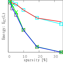
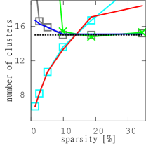
(c) Purity	(d) Run time
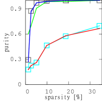
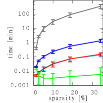
Legend: Swap-and-Explore, Expand-and-Explore, ICM, TRW-S, BP

Figure 42: Synthetic results: Graphs comparing (a) Energy at convergence. (b) Recovered number of clusters. (c) Purity of resulting clusters. (d) Run time of algorithms (log scale). TRW-S and BP are almost indistinguishable, as are Swap and Expand in most of the plots.

This experiment uses synthetic affinity matrices $W$ to compare our algorithms to existing Potts optimization algorithms. The synthetic data have 750 variables randomly assigned to 15 clusters with different sizes (ratio between larger to smaller cluster: $\sim\times 5$). For each variable we sampled roughly the same number of neighbors: of which $\sim 25\%$ are from within the cluster and the rest from the other clusters. We corrupted the clean ground-truth adjacency matrix with $20\%$ noise affecting both the sign of $W_{ij}$ and the certainty (i.e., $\left|W_{ij}\right|$). Overall the resulting percent of positive (submodular) connections is $\sim 30\%$.

We report several measurements for these experiments: run-time, energy ($\mathcal{E}_{CC}$), purity of the resulting clusters and the recovered number of clusters $k$ for each of the algorithms as a function of the sparsity of the matrix $W$, i.e., percent of non-zero entries. Each experiment was repeated $10$ times with different randomly generated matrices.

Fig. 42 shows results of the synthetic experiments. Existing multi-label approaches (TRW-S and BP) do not perform too well: higher $\mathcal{E}_{CC}$, lower purity and incorrect recovery of $k$. This demonstrates the difficulty of the energy minimization problem that has no unary term and many non-submodular pair-wise terms. These results are in accordance with the observations of Kolmogorov and Wainwright (2005) when the energy is hard to optimize.

For our large move making algorithms, Expand-and-Explore provides marginally better clustering results than the Swap-and-Explore. However, its relatively slow running time makes it infeasible for large CC problems. A somewhat surprising result of these experiments shows that for matrices not too sparse (above $10\%$), adaptive-label ICM performs surprisingly well. In fact, it is significantly faster than all the other methods and manages to converge to the correct number of clusters with high purity and low energy.

From these experiments we conclude that Swap-and-Explore (Alg. 2) is a very good choice of optimization algorithm for the CC functional. However, when the affinity matrix $W$ is not too sparse, it is worth while giving our adaptive-label ICM a shot.

34.2 Co-clustering data

The following experiment compares our algorithms with a state-of-the-art CC optimization method, R-LP, of Vitaladevuni and Basri (2010). For this comparison we use affinity matrices computed for co-segmentation. The co-segmentation problem can be formulated as a correlation clustering problem with super pixels as the variables (Glasner et al. (2011)).

We obtained 77 affinity matrices, courtesy of Glasner et al. (2011), used in their experiments. The number of variables in each matrix ranges from 87 to 788, Their sparsity (percent of non-zero entries) ranges from $6\%$ to $50\%$, and there are roughly the same number of positive (submodular) and negative (non-submodular) entries.

Table 6 shows the ratio between our energy and the energy of R-LP method. The table also shows the percent of matrices for which our algorithms found a solution with lower energy than R-LP. The results show the superiority of our algorithms to existing multi-label energy minimization approaches (TRW-S and BP). Furthermore, it is shown that our methods are in par with existing state-of-the-art CC optimization method on small problems. However, unlike existing methods, our algorithms can be applied to problems two orders of magnitude larger. Optimizing directly for $U$ not only did not compromise the performance of our method, but also allows us to handle large scale CC optimization, as demonstrated in the next section.

	Ours
	Swap	Expand	ICM	TRWS	BP
Energy ratio	$98.6$	$98.4$	$77.4$	$83.8$	$83.6$
(%)	$\pm 1.4$	$\pm 1.9$	$\pm 23.9$	$\pm 5.4$	$\pm 6.3$
Strictly lower	15%	11.7%	0	0	0
$\left(>100\%\right)$

Table 6: Comparison to Glasner et al. (2011): Ratio between our energy and of Glasner et al.: Since all energies are negative, higher ratio means lower energy. Ratio higher than $100\%$ means our energy is better than Glasner et al.. Bottom row shows the percentage of cases where each method got strictly lower energy than Glasner et al..

35 Conclusion

This work suggests a new perspective on the functional, viewing it as a discrete Potts energy. The resulting energy minimization presents three challenges: (i) the energy is non submodular, (ii) the number of clusters is not known in advance, and (iii) there is no unary term. We proposed new energy minimization algorithms that can successfully cope with these challenges.

Chapter 8 Discrete Multiscale Optimization

This chapter presents a unified multiscale framework for discrete energy minimization that directly acts on the energy. Our approach utilizes algebraic multiscale principles to efficiently explore the discrete solution space. The main goal of our framework is to improve optimization performance for challenging, non-submodular energies for which current methods provide unsatisfactory approximations. Furthermore, the ability to derive a multiscale pyramid directly from an energy makes our framework application independent. Two important implications rise from this independence: (i) One no longer needs to tailor a multiscale scheme to suit each different application. (ii) Our framework makes it trivial to turn existing single scale optimization algorithms into powerful multiscale methods. Our framework gives rise to two complementary energy coarsening strategies: one in which coarser scales involve fewer variables, and a more revolutionary one in which the coarser scales involve fewer discrete labels. We empirically evaluated our unified framework on a variety of both non-submodular and submodular energies, including energies from the Middlebury benchmark.

36 Introduction

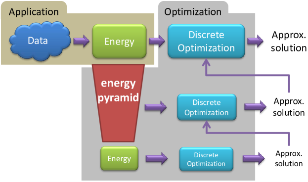
Figure 43: A Unified multiscale framework: We derive multiscale representation of the energy itself = energy pyramid. Our multiscale framework is unified in the sense that different problems with different energies share the same multiscale scheme, making our framework widely applicable and general.

Discrete energy minimization is ubiquitous in computer vision, and spans a variety of problems such as segmentation, denoising, stereo, etc. Unfortunately, apart from the submodular binary case, minimizing these energies is known to be NP-hard. A lot of effort is recently put on developing algorithms for approximate discrete optimization for ever more challenging energies: multi-label, non-submodular, etc. (e.g., Szeliski et al. (2008); Kolmogorov (2006); Bagon and Galun (2011)).

Discrete energies may be grossly divided into two categories: submodular (regular) energies and non-submodular energies. Submodular energies are characterized by smoothness-encouraging pair-wise (and higher order) terms. These energies reflect the “piece-wise constant” prior that is very popular and common in computer vision applications. For this reason most of the effort and research regarding discrete optimization, in the context of computer vision, focuses on these energies with encouraging results. In practice, despite the NP-hardness of these energies, algorithms were developed that provide solutions with energies close to global optimum (e.g., Kolmogorov (2006); Boykov et al. (2001)). Therefore we consider this type of energies as “easy to optimize”.

In contrast, non-submodular energies are characterized by contrast-encouraging pair wise terms. These energies may be encountered when the parameters of the energy are learned (e.g., Nowozin et al. (2011)), or when different functionals are used (e.g., Bagon and Galun (2011); Glasner et al. (2011)). When it comes to optimization it is generally considered a more challenging task to optimize a non-submodular energies. Since these examples of non-submodular energies are only recently explored, their optimization receives less attention, and consequently, the existing optimization methods provide approximations that may be quite unsatisfactory. We consider these energies as “hard to optimize”.

Algorithms for discrete energy minimization may also be classified into two categories: primal methods and dual methods. Primal methods act directly on the discrete variables in the label space to minimize the energy (e.g., Besag (1986); Boykov et al. (2001)). In contrast, dual methods formulate a dual problem to the energy and maximize a lower bound to the sought energy (e.g., Kolmogorov (2006)). Dual methods are recently considered more favorable since they not only provide an approximate solution, but also provide a lower bound on how far this solution is from the global optimum. Furthermore, if a labeling is found with energy equals to the lower bound a certificate is provided that the global optimum was found.

Since most of the relevant discrete optimization problems are NP-hard, one can only provide an empirical evaluation of how well a given algorithm approximates representative instances of these energies. For the submodular, “easy to optimize”, energies it was shown (by Szeliski et al. (2008)) that dual methods tend to provide better approximations with very tight lower bounds.

[r][r] But what makes discrete energy minimization such a challenging endeavor? The fact that this minimization implies an exploration of an exponentially large search space makes it such a challenging task. One way to alleviate this difficulty is to use multiscale search. The illustration on the right shows a toy “energy” $E(L)$ at different scales of detail. Considering only the original scale ($s=0$), it is very difficult to suggest an effective exploration/optimization method. However, when looking at coarser scales ($s=1,\ldots,3$) of the energy an interesting phenomenon is revealed. At the coarsest scale ($s=3$) the large basin of attraction emerges, but with very low accuracy. As the scales become finer ($s=2,\ldots,0$), one “loses sight” of the large basin, but may now “sense” more local properties with higher accuracy. We term this well known phenomenon as the multiscale landscape of the energy. This multiscale landscape phenomenon encourages coarse-to-fine exploration strategies: starting with the large basins that are apparent at coarse scales, and then gradually and locally refining the search at finer scales.

For more than three decades the vision community has focused on the multiscale pyramid of the image (e.g., Lucas and Kanade (1981); Burt and Adelson (1983)). There is almost no experience and no methods that apply a multiscale scheme directly to the discrete energy.

In this paper we present a novel unified discrete multiscale optimization scheme that acts directly on the energy (Fig. 43). Our approach allows for an efficient exploration of the discrete solution space through the construction of an energy pyramid. Moreover, our multiscale framework is application independent: different problems with different energies share the same multiscale scheme, making our framework widely applicable and general.

Performing empirical evaluations of non-submodular energies minimization lead us to conclude that when it comes to hard to optimize non-submodular energies, primal methods tend to provide better approximations than dual methods. Motivated by this observation, we formulate out multiscale framework in the primal space (i.e., expressing it in terms of the variables and labels directly). Our multiscale framework becomes the core of the optimization process allowing for existing “off-the-shelf” primal optimization algorithms to efficiently exploit the multiscale landscape of the energy and achieves significantly lower energies faster.

This work makes several contributions:

1. A novel unified multiscale framework for discrete optimization. A wide variety of optimization problems, including segmentation, stereo, denoising, correlation-clustering, and others share the same multiscale framework.

2. Energy-aware coarsening scheme. Variable aggregation takes into account the underlying structure of the energy itself, thus efficiently and directly exposes its multiscale landscape.

3. Coarsening the labels. Our formulation allows for variable aggregation as well as for label coarsening. This yields an energy pyramid with fewer labels at the coarser scales.

4. Integrating existing single-scale optimization algorithms into our multiscale framework. We achieve significantly lower energy assignments on diverse computer vision energies, including challenging non-submodular examples.

5. Optimizing hard non-submodular energies. Using several classes of non-submodular energies, we empirically exemplify the superiority of primal methods. We further show how combining in our multiscale framework single-scale primal optimization methods achieve increased optimization performance on these challenging problems.

36.1 Related work

There are very few works that apply multiscale schemes directly to the energy. A prominent example for this approach is that of Felzenszwalb and Huttenlocher (2006), that provide a coarse-to-fine belief propagation scheme restricted to regular diadic pyramid. A more recent work is that of Komodakis (2010) that provides an algebraic multigrid formulation for discrete optimization in the dual space. However, despite his general formulation Komodakis only provides examples using regular diadic grids of easy to optimize submodular energies.

The work of Kim et al. (2011) proposes a two-scales scheme mainly aimed at improving run-time of the optimization process. Their proposed coarsening strategies can be interpreted as special cases of our unified framework. We analyze their underlying assumptions (Sec. 38.1), and suggest better methods for efficient exploration of the multiscale landscape of the energy.

A different approach for discrete optimization suggests large move making algorithms (e.g., Boykov et al. (2001); Swendsen and Wang (1987)). We experimentally show how plugging such methods within our multiscale framework improves optimization results. These methods do not scale gracefully with the number of labels. Lempitsky et al. (2007) proposed a method to exploit known properties of the metric between the labels to allow for faster minimization of the energy. However, their method is restricted to energies with clear and known label metrics and requires training. In contrast, our framework addresses this issue via a principled scheme that builds an energy pyramid with a decreasing number of labels without prior training and with fewer assumptions on the labels interactions.

37 Multiscale Energy Pyramid

In this work we consider discrete pair-wise minimization problems, defined over a (weighted) graph $\left(\mbox{$\mathcal{V}$},\mbox{$\mathcal{E}$}\right)$, of the form:

$$E\left(L\right) = \sum_{i\in\mbox{$\mathcal{V}$}}\psi_{i}\left(l_{i}\right)+\sum_{\left(i,j\right)\in\mbox{$\mathcal{E}$}}w_{ij}\cdot\psi\left(l_{i},l_{j}\right)$$ (49)

where $\mathcal{V}$ is the set of variables, $\mathcal{E}$ is the set of edges, and the solution is discrete: $L\in\left\{1,\ldots,l\right\}^{n}$, with $n$ variables taking $l$ possible labels. Many problems in computer vision are cast in the form of (49) (see Szeliski et al. (2008)). Furthermore, we do not restrict the energy to be submodular, and our framework is also applicable to more challenging non-submodular energies.

Our aim is to build an energy pyramid with a decreasing number of degrees of freedom. The key component in constructing such a pyramid is the interpolation method. The interpolation maps solutions between levels of the pyramid, and defines how to approximate the original energy with fewer degrees of freedom. We propose a novel principled energy aware interpolation method. The resulting energy pyramid exposes the multiscale landscape of the energy making low energy assignments apparent at coarse levels.

However, it is counter intuitive to directly interpolate discrete values, since they usually have only semantic interpretation. Therefore, we substitute an assignment $L$ by a binary matrix $U\in\left\{0,1\right\}^{n\times l}$. The rows of $U$ correspond to the variables, and the columns corresponds to labels: $U_{i,\alpha}=1$ iff variable $i$ is labeled “$\alpha$” ($l_{i}=\alpha$). This representation allows us to interpolate discrete solutions, as will be shown in the subsequent sections.

Expressing the energy (49) using $U$ yields a relaxed quadratic representation (along the lines of Rangarajan (2000)) that forms the basis for our multiscale framework derivation:

$$E\left(U\right) = Tr\left(DU^{T}+WUVU^{T}\right)$$ (50)

s.t. $$U\in\left\{0,1\right\}^{n\times l},\ \sum_{\alpha=1}^{l}U_{i\alpha}=1$$ (51)

where $W$ is sparse with entries $\left\{w_{ij}\right\}$, $D\in\mathbb{R}^{n\times l}$ s.t. $D_{i,\alpha}\mbox{$\stackrel{{\scriptstyle\mbox{\tiny{def}}}}{{=}}$}\psi_{i}(\alpha)$, and $V\in\mathbb{R}^{l\times l}$ s.t. $V_{\alpha,\beta}\mbox{$\stackrel{{\scriptstyle\mbox{\tiny{def}}}}{{=}}$}\psi\left(\alpha,\beta\right)$, $\alpha,\beta\in\left\{1,\ldots,l\right\}$. A detailed derivation of (50) can be found in Sec. 8.A.

An energy over $n$ variables with $l$ labels is now parameterized by $\left(n,l,D,W,V\right)$.

We first describe the energy pyramid construction for a given interpolation matrix $P$, and defer the detailed description of our novel interpolation to Sec. 38.

Energy coarsening by variables

Let $\left(n^{f},l,D^{f},W^{f},V\right)$ be the fine scale energy. We wish to generate a coarser representation $\left(n^{c},l,D^{c},W^{c},V\right)$ with $n^{c}<n^{f}$. This representation approximates $E\left(U^{f}\right)$ using fewer variables: $U^{c}$ with only $n^{c}$ rows.

Given an interpolation matrix $P\in\left[0,1\right]^{{n^{f}}\times{n^{c}}}$ s.t. $\sum_{j}P_{ij}=1$ $\forall i$, it maps coarse to fine assignments through:

$$U^{f} \approx PU^{c}$$ (52)

For any fine assignment that can be approximated by a coarse assignment $U^{c}$ we may plug (52) into (50) yielding:

$$E\left(U^{f}\right) = Tr\left(D^{f}{U^{f}}^{T}+W^{f}U^{f}V{U^{f}}^{T}\right)$$ (53)

$$\approx Tr\left(D^{f}{U^{c}}^{T}P^{T}+W^{f}PU^{c}V{U^{c}}^{T}P^{T}\right)$$

$$= Tr\Big{(}\underbrace{\left(P^{T}D^{f}\right)}_{\mbox{\normalsize$\mbox{$\stackrel{{\scriptstyle\mbox{\tiny{def}}}}{{=}}$}D^{c}$ }}{U^{c}}^{T}+\underbrace{\left(P^{T}W^{f}P\right)}_{\mbox{\normalsize$\mbox{$\stackrel{{\scriptstyle\mbox{\tiny{def}}}}{{=}}$}W^{c}$}}U^{c}V{U^{c}}^{T}\Big{)}$$

$$= Tr\left(D^{c}{U^{c}}^{T}+W^{c}U^{c}V{U^{c}}^{T}\right)$$

$$= E\left(U^{c}\right)$$

We have generated a coarse energy $E\left(U^{c}\right)$ parameterized by $\left(n^{c},l,D^{c},W^{c},V\right)$ that approximates the fine energy $E(U^{f})$. This coarse energy is of the same form as the original energy allowing us to apply the coarsening procedure recursively to construct an energy pyramid.

Energy coarsening by labels

So far we have explored the reduction of the number of degrees of freedom by reducing the number of variables. However, we may just as well look at the problem from a different perspective: reducing the search space by decreasing the number of labels from $l_{f}$ to $l_{c}$ ($l_{c}<l_{f}$). It is a well known fact that optimization algorithms (especially large move making, e.g., Boykov et al. (2001)) suffer from significant degradation in performance as the number of labels increases (Bleyer et al. (2010)). Here we propose a novel principled and general framework for reducing the number of labels at each scale.

Let $\left(n,l^{f},D^{\hat{f}},W,V^{\hat{f}}\right)$ be the fine scale energy. Looking at a different interpolation matrix $\hat{P}\in\left[0,1\right]^{\mbox{$l^{f}\times l^{c}$}}$, we may interpolate a coarse solution by $U^{\hat{f}}\approx U^{\hat{c}}\hat{P}^{T}$. This time the interpolation matrix $\hat{P}$ acts on the labels, i.e., the columns of $U$. The coarse labeling matrix $U^{\hat{c}}$ has the same number of rows (variables), but fewer columns (labels). We use $\hat{\Box}$ notation to emphasize that the coarsening here affects the labels rather than the variables.

Coarsening the labels yields:

$$E\left(U^{\hat{c}}\right)=Tr\left(\left(D^{\hat{f}}\hat{P}\right)\mbox{$U^{\hat{c}}$}^{T}+WU^{\hat{c}}\left(\hat{P}^{T}V^{\hat{f}}\hat{P}\right)\mbox{$U^{\hat{c}}$}^{T}\right)$$ (54)

Again, we end up with the same type of energy, but this time it is defined over a smaller number of discrete labels: $\left(n,l^{c},D^{\hat{c}},W,V^{\hat{c}}\right)$, where $D^{\hat{c}}\mbox{$\stackrel{{\scriptstyle\mbox{\tiny{def}}}}{{=}}$}D^{\hat{f}}\hat{P}$ and $V^{\hat{c}}\mbox{$\stackrel{{\scriptstyle\mbox{\tiny{def}}}}{{=}}$}\hat{P}^{T}V^{\hat{f}}\hat{P}$.

The main theoretical contribution of this work is encapsulated in the multiscale “trick” of equations (53) and (54). This formulation forms the basis of our unified framework allowing us to coarsen the energy directly and exploits its multiscale landscape for efficient exploration of the solution space. This scheme moves the multiscale completely to the optimization side and makes it independent of any specific application. We can practically now approach a wide and diverse family of energies using the same multiscale implementation.

The effectiveness of the multiscale approximation of (53) and (54) heavily depends on the interpolation matrix $P$ ($\hat{P}$ resp.). Poorly constructed interpolation matrices will fail to expose the multiscale landscape of the functional. In the subsequent section we describe our principled energy-aware method for computing it.

38 Energy-aware Interpolation

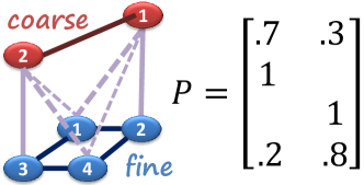
Figure 44: Interpolation as soft variable aggregation: fine variable 1, 2 and 4 are aggregated into coarse variable 1, while fine variables 1,3 and 4 are aggregated into coarse variable 2. Soft aggregation allows for fine variables to be influenced by few coarse variables, e.g.: fine variable 1 is a convex combination of $.7$ of 1 and $.3$ of 2. Hard aggregation is a special case where $P$ is a binary matrix. In that case each fine variable is influenced by exactly one coarse variable.

In this section we use terms and notations for variable coarsening ($P$), however the motivation and methods are applicable for label coarsening ($\hat{P}$) as well due to the similar algebraic structure of (53) and (54).

Our energy pyramid approximates the original energy using a decreasing number of degrees of freedom, thus excluding some solutions from the original search space at coarser scales. Which solutions are excluded is determined by the interpolation matrix $P$. A desired interpolation does not exclude low energy assignments at coarse levels.

The matrix $P$ can be interpreted as an operator that aggregates fine-scale variables into coarse ones (Fig. 44). Aggregating fine variables $i$ and $j$ into a coarser one excludes from the search space all assignments for which $l_{i}\neq l_{j}$. This aggregation is undesired if assigning $i$ and $j$ to different labels yields low energy. However, when variables $i$ and $j$ are strongly correlated by the energy (i.e., assignments with $l_{i}=l_{j}$ yield low energy), aggregating them together efficiently allows exploration of low energy assignments. A desired interpolation aggregates $i$ and $j$ when $i$ and $j$ are strongly correlated by the energy.

38.1 Measuring energy-aware correlations

We provide two correlations measures, one used in computing variable coarsening ($P$) and the other used for label coarsening ($\hat{P}$).

Energy-aware correlations between variables: A reliable estimation for the correlations between the variables allows us to construct a desirable $P$ that aggregates strongly correlated variables. A naïve approach would assume that neighboring variables are correlated (this assumption underlies Felzenszwalb and Huttenlocher (2006)). This assumption clearly does not hold in general and may lead to an undesired interpolation matrix $P$. Kim et al. (2011) proposed several “closed form formulas” for energy-aware variable grouping. However, their formulas take into account either the unary term or the pair-wise term. Indeed it is difficult to decide which term dominates and how to fuse these two terms together. Therefore, there is no “closed form” method that successfully integrates both of them.

As opposed to these “closed form” methods, we propose a novel empirical scheme for correlation estimation. Empirical estimation of the correlations naturally accounts for and integrates the influence of both the unary and the pair-wise terms. Moreover, our method, inspired by Ron et al. (2011); Livne and Brandt (2011), extends to all energies (50): submodular, non-submodular, metric $V$, arbitrary $V$, arbitrary $W$, energies defined over regular grids and arbitrary graphs.

Variables $i$ and $j$ are correlated by the energy when $l_{i}=l_{j}$ yields relatively low energy value. To estimate these correlations we empirically generate several “locally” low energy assignments, and measure the label agreement between neighboring variables $i$ and $j$. We use Iterated Conditional Modes (ICM) of Besag (1986) to obtain locally low energy assignments: Starting with a random assignment, ICM chooses, at each iteration and for each variable, the label yielding the largest decrease of the energy function, conditioned on the labels assigned to its neighbors.

Performing $t=10$ ICM iterations for $K=10$ random initializations provides $K$ locally low energy assignments $\left\{L^{k}\right\}_{k=1}^{K}$. Our empirical dissimilarity between $i$ and $j$ is given by $d_{ij}=\frac{1}{K}\sum_{k}V_{l^{k}_{i},l^{k}_{j}}$, and their correlation is given by $c_{ij}=\exp\left(-\frac{d_{ij}}{\sigma}\right)$, with $\sigma\propto\max V$.

It is interesting to note that strong correlation between variables $i$ and $j$ usually implies that the pair-wise term binding them together ($\varphi_{ij}$) is a smoothness-preserving type of relation. We assume that even for challenging energies with many contrast-enhancing pair-wise terms, there are still significant amount of smoothness-preserving terms to allow for effective coarsening.

Energy-aware correlations between labels: Correlations between labels are easier to estimate, since this information is explicit in the matrix $V$ that encodes the “cost” (i.e., dissimilarity) between two labels. Setting $\hat{c}_{\alpha,\beta}\propto\left(\hat{V}_{\alpha,\beta}\right)^{-1}$, we get a “closed-form” expression for the correlations between labels.

38.2 From correlations to interpolation

Using our measure for the variable correlations, $c_{ij}$, we follow the Algebraic Multigrid (AMG) method of Brandt (1986) to compute an interpolation matrix $P$ that softly aggregates strongly correlated variables.

We begin by selecting a set of coarse representative variables $\mbox{$\mathcal{V}$}^{c}\subset\mbox{$\mathcal{V}$}^{f}$, such that every variable in $\mbox{$\mathcal{V}$}^{f}\backslash\mbox{$\mathcal{V}$}^{c}$ is strongly correlated with $\mbox{$\mathcal{V}$}^{c}$. That is, every variable in $\mbox{$\mathcal{V}$}^{f}$ is either in $\mbox{$\mathcal{V}$}^{c}$ or is strongly correlated to other variables in $\mbox{$\mathcal{V}$}^{c}$. A variable $i$ is considered strongly correlated to $\mbox{$\mathcal{V}$}^{c}$ if $\sum_{j\in\mbox{$\mathcal{V}$}^{c}}c_{ij}\geq\beta\sum_{j\in\mbox{$\mathcal{V}$}^{f}}c_{ij}$. $\beta$ affects the coarsening rate, i.e., the ratio $n^{c}/n^{f}$, smaller $\beta$ results in a lower ratio. We perform this selection greedily and sequentially, starting with $\mbox{$\mathcal{V}$}^{c}=\emptyset$ adding $i$ to $\mbox{$\mathcal{V}$}^{c}$ if it is not yet strongly correlated to $\mbox{$\mathcal{V}$}^{c}$.

Given the selected coarse variables $\mbox{$\mathcal{V}$}^{c}$, $I(j)$ maps indices of variables from fine to coarse: $I(j)$ is the coarse index of the variable whose fine index is $j$ (in Fig. 44: $I(2)=1$ and $I(3)=2$). The interpolation matrix $P$ is defined by:

$$P_{iI(j)}=\left\{\begin{array}[]{cl}c_{ij}&i\in\mbox{$\mathcal{V}$}^{f}\backslash\mbox{$\mathcal{V}$}^{c},\ j\in\mbox{$\mathcal{V}$}^{c}\\ 1&i\in\mbox{$\mathcal{V}$}^{c},j=i\\ 0&\mbox{otherwise}\\ \end{array}\right.$$ (55)

We further prune rows of $P$ leaving only $\delta$ maximal entries. Each row is then normalized to sum to 1. Throughout our experiments we use $\beta=0.2$ ($\hat{\beta}=0.75$), $\delta=3$ ($\hat{\delta}=2$) for computing $P$ ($\hat{P}$ resp.).

39 Unified Discrete Multiscale Framework

Input: Energy $\left(\mbox{$\mathcal{V}$}^{0},D^{0},W^{0},V\right)$.

Output: $U^{0}$

Init $s\leftarrow 0$// fine scale

// Energy pyramid construction:

while $\mbox{$\left|\mbox{$\mathcal{V}$}^{s}\right|$}\geq 10$ do

       Estimate pair-wise correlations $c_{ij}$ at scale $s$ (Sec. 38.1).

       Compute interpolation matrix $P^{s}$ (Sec. 38.2).

       Derive coarse energy $\left(\mbox{$\mathcal{V}$}^{s+1},D^{s+1},W^{s+1},V\right)$ (Eq. 53).

       $s++$

      

// Coarse-to-fine optimization:

while $s\geq 0$ do

       $U^{s}\leftarrow$ Refine $(\tilde{U}^{s})$

       $\tilde{U}^{s-1}=P^{s}U^{s}$// interpolate a solution

       $s--$

      

where Refine $(\tilde{U}^{s})$ uses an “off-the-shelf” algorithm to optimize the energy $\left(\mbox{$\mathcal{V}$}^{s},D^{s},W^{s},V\right)$ with $\tilde{U}^{s}$ as an initialization.

Algorithm 3 Discrete multiscale optimization.

So far we have described the different components of our multiscale framework. Alg. 3 puts them together into a multiscale minimization scheme. Given an energy $\left(\mbox{$\mathcal{V}$},D,W,V\right)$, our framework first works fine-to-coarse to compute interpolation matrices $\left\{P^{s}\right\}$ that generates an “energy pyramid”. Typically we end up at the coarsest scale with less than $10$ variables. As a result, exploring the energy at this scale is robust to the initial assignment of the single-scale method used.

Starting from the coarsest scale, a coarse solution at scale $s$ is interpolated to a finer scale $s-1$. At the finer scale it serves as a good initialization for an “off-the-shelf” single-scale optimization that refines this interpolated solution. These two steps are repeated for all scales from coarse to fine.

The interpolated solution $\tilde{U}^{s-1}$, at each scale, might not satisfy the binary constraints (51). We round each row of $\tilde{U}^{s-1}$ by setting the maximal element to $1$ and the rest to $0$.

The most computationally intensive modules of our framework are the empirical estimation of the variable correlations and the single-scale optimization used to refine the interpolated solutions. The complexity of the correlation estimation is $O\left(\mbox{$\left|\mbox{$\mathcal{E}$}\right|$}\cdot l\right)$, where $\left|\mbox{$\mathcal{E}$}\right|$ is the number of non-zero elements in $W$ and $l$ is the number of labels. However, it is fairly straightforward to parallelize this module.

It is now easy to see how our framework generalizes Felzenszwalb and Huttenlocher (2006), Komodakis (2010) and Kim et al. (2011): They are restricted to hard aggregation in $P$. Felzenszwalb and Huttenlocher (2006) and Komodakis (2010) use a multiscale pyramid, however their variable aggregation is not energy-aware, and is restricted to diadic pyramids. On the other hand, Kim et al. (2011) have limited energy-aware aggregation, applied to a two level only “pyramid”. They only optimize at the coarse scale and cannot refine the solution on the fine scale.

40 Experimental Results

Our experiments has two main goals: first, to stress the difficulty of approximating non-submodular energies and to show the advantages of primal methods for this type of minimization problems. The other goal is to demonstrate how our unified multiscale framework improved the performance of existing single-scale primal methods.

We evaluated our multiscale framework on a diversity of discrete optimization tasks: ranging from challenging non-submodular synthetic and co-clustering energies to low-level submodular vision energies such as denoising and stereo. In addition we provide a comparison between the different methods for measuring variable correlations that were presented in Sec. 38.1. We conclude with a label coarsening experiment. In all of these experiments we minimize a given publicly available benchmark energy, we do not attempt to improve on the energy formulation itself.

We use ICM (Besag (1986)), $\alpha\beta$-swap and $\alpha$-expansion (large move making algorithms of Boykov et al. (2001)) as representative single-scale “off-the-shelf” primal optimization algorithms. To help large move making algorithms to overcome the non-submodularity of some of these energies we augment them with QPBO(I) of Rother et al. (2007).

We follow the protocol of Szeliski et al. (2008) that uses the lower bound of TRW-S (Kolmogorov (2006)) as a baseline for comparing the performance of different optimization methods for different energies. We report how close the results (in percents) to the lower bound: closer to $100\%$ is better.

We show a remarkable improvement for ICM combined in our multiscale framework compared with a single-scale scheme. For the large move making algorithms there is a smaller but consistent improvement of the multiscale over a single scale scheme. TRW-S is a dual method and is considered state-of-the-art for discrete energy minimization Szeliski et al. (2008). However, we show that when it comes to non-submodular energies it struggles behind the large move making algorithms and even ICM. For these challenging energies, multiscale gives a significant boost in optimization performance.

$\lambda$	ICM		Swap		Expand		TRW-S
	Ours	single	Ours	single	Ours	single
		scale		scale		scale
$5$	$112.6\%$	$115.9\%$	$108.9\%$	$110.0\%$	$110.5\%$	$110.0\%$	$116.6\%$
$10$	$123.6\%$	$130.2\%$	$118.5\%$	$120.2\%$	$121.5\%$	$121.0\%$	$134.6\%$
$15$	$127.1\%$	$135.8\%$	$122.1\%$	$124.1\%$	$124.6\%$	$125.1\%$	$138.3\%$

Table 7: Synthetic results (energy): Showing percent of achieved energy value relative to the lower bound (closer to $100\%$ is better) for ICM, $\alpha\beta$-swap, $\alpha$-expansion and TRW-S for varying strengths of the pair-wise term ($\lambda=5,\ldots,15$, stronger $\rightarrow$ harder to optimize.)

40.1 Synthetic

We begin with synthetic non-submodular energies defined over a 4-connected grid graph of size $50\times 50$ ($n=2500$), and $l=5$ labels. The unary term $D\sim\mathcal{N}\left(0,1\right)$. The pair-wise term $V_{\alpha\beta}=V_{\beta\alpha}\sim\mathcal{U}\left(0,1\right)$ ($V_{\alpha\alpha}=0$) and $w_{ij}=w_{ji}\sim\lambda\cdot\mathcal{U}\left(-1,1\right)$. The parameter $\lambda$ controls the relative strength of the pair-wise term, stronger (i.e., larger $\lambda$) results with energies more difficult to optimize (see Kolmogorov (2006)). Table 7 shows results, averaged over 100 experiments.

The resulting synthetic energies are non-submodular (since $w_{ij}$ may become negative). For these challenging energies, state-of-the-art dual method (TRW-S) performs rather poorly (worse than single scale ICM) and there is a significant gap between the lower bound and the energy of the actual primal solution provided. Among the primal methods used, These results motivate our focusing on primal methods, especially $\alpha\beta$-swap.

GT	Input	ICM		QPBO		TRW-S	Sim.
		Ours	single	Ours	single		Ann.
			scale		scale

Figure 45: Chinese characters inpainting: Visualizing some of the instances used in our experiments. Columns are (left to right): The original character used for testing. The input partially occluded character. ICM and QPBO results both our multiscale and single scale results. Results of TRW-S and results of Nowozin et al. (2011) obtained with a very long run of simulated annealing (using Gibbs sampling inside the annealing).

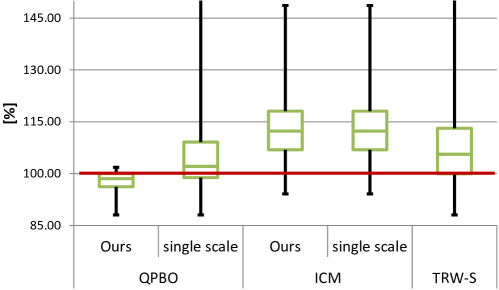
Figure 46: Energies of Chinese characters inpainting: Box plot showing 25%, median and 75% of the resulting energies relative to reference energies of Nowozin et al. (2011) (lower than $100\%$ = lower than baseline). Our multiscale approach combined with QPBO achieves consistently better energies than baseline, with very low variance. TRW-S improves on only 25% of the instances with very high variance in the results.

	ICM		QPBO		TRW-S
	Ours	single-scale	Ours	single-scale
(a)	$114.0\%$	$114.0\%$	$97.8\%$	$106.2\%$	$108.6\%$
(b)	$7.0\%$	$7.0\%$	$77.0\%$	$34.0\%$	$25.0\%$

Table 8: Energies of Chinese characters inpainting: table showing (a) mean energies for the inpainting experiment relative to baseline of Nowozin et al. (2011) (lower is better, less than $100\%$ = lower than baseline). (b) percent of instances for which strictly lower energy was achieved.

40.2 Chinese character inpainting

We further experiment with learned binary energies of (Nowozin et al., 2011, §5.2). These 100 instances of non-submodular pair-wise energies are defined over a 64-connected grid. These energies were designed and trained to perform the task of learning Chinese calligraphy, represented as a complex, non-local binary pattern. Despite the very large number of parameters involved in representing such complex energies, learning is conducted very efficiently using Decision Tree Field (DTF). The main challenge in these models becomes the inference at test time.

Our experiments show how approaching these challenging energies using our unified multiscale framework allows for better approximations. Table 8 and Fig. 45 compare our multiscale framework to single-scale methods acting on the primal binary variables. Since the energies are binary, we use QPBO instead of large move making algorithms. We also provide an evaluation of a dual method (TRW-S) on these energies. In addition to the quantitative results, Fig. 46 provides a visualization of some of the instances of the restored Chinese characters.

These “real world” energies highlight the advantage primal methods has over dual ones when it comes to challenging non-submodular energies. It is further clear that significant improvement is made by our multiscale framework.

	ICM		Swap		Expand		TRW-S
	Ours	single	Ours	single	Ours	single
		scale		scale		scale
(a)	$99.9\%$	$177.7\%$	$99.8\%$	$101.5\%$	$99.8\%$	$101.6\%$	$176.2\%$
(b)	$55.6\%$	$0.0\%$	$71.8\%$	$15.5\%$	$70.8\%$	$11.6\%$	$0.5\%$

Table 9: Co-clustering results: Baseline for comparison are state-of-the-art results of Glasner et al. (2011). (a) We report our results as percent of the baseline: smaller is better, lower than $100\%$ even outperforms state-of-the-art. (b) We also report the fraction of energies for which our multiscale framework outperform state-of-the-art.

40.3 Co-clustering

The problem of co-clustering addresses the matching of superpixels within and across frames in a video sequence. Following (Bagon and Galun, 2011, §6.2), we treat co-clustering as a discrete minimization of non-submodular Potts energy. We obtained 77 co-clustering energies, courtesy of Glasner et al. (2011), used in their experiments. The number of variables in each energy ranges from 87 to 788. Their sparsity (percent of non-zero entries in $W$) ranges from $6\%$ to $50\%$, The resulting energies are non-submodular, have no underlying regular grid, and are very challenging to optimize Bagon and Galun (2011).

Table 9 compares our discrete multiscale framework combined with ICM and $\alpha\beta$-swap. For these energies we use a different baseline: the state-of-the-art results of Glasner et al. (2011) obtained by applying specially tailored convex relaxation method (We do not use the lower bound of TRW-S here since it is far from being tight for these challenging energies). Our multiscale framework improves state-of-the-art for this family of challenging energies.

40.4 semi-metric energies

We further applied our multiscale framework to optimize less challenging semi-metric energies. We use the diverse low-level vision MRF energies from the Middlebury benchmark Szeliski et al. (2008).

For these semi-metric energies, TRW-S (single scale) performs quite well and in fact, if enough iterations are allowed, its lower bound converges to the global optimum. As opposed to TRW-S, large move making and ICM do not always converge to the global optimum. Yet, we are able to show a significant improvement for primal optimization algorithms when used within our multiscale framework. Tables 10 and 11 and Figs. 47 and 48 show our multiscale results for the different submodular energies.

One of the conclusions of the Middlebury challenge was that ICM is no longer a valid candidate for optimization. Integrating ICM into our multiscale framework puts it back on the right track.

	ICM		Swap		Expand
	Ours	single scale	Ours	single scale	Ours	single scale
Tsukuba	$102.8\%$	$653.4\%$	$100.2\%$	$100.5\%$	$100.1\%$	$100.3\%$
Venus	$112.3\%$	$405.1\%$	$102.8\%$	$128.7\%$	$102.7\%$	$102.8\%$
Teddy	$102.5\%$	$234.3\%$	$100.4\%$	$100.8\%$	$100.3\%$	$100.5\%$

Table 10: Stereo: Showing percent of achieved energy value relative to the lower bound (closer to $100\%$ is better). Visual results for these experiments are in Fig. 47. Energies from Szeliski et al. (2008).

ICM		Swap		Expand		Ground
Ours	Single scale	Ours	Single scale	Ours	Single scale	truth

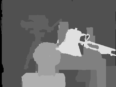
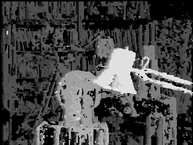
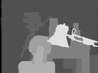
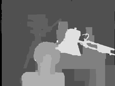
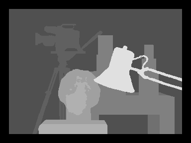
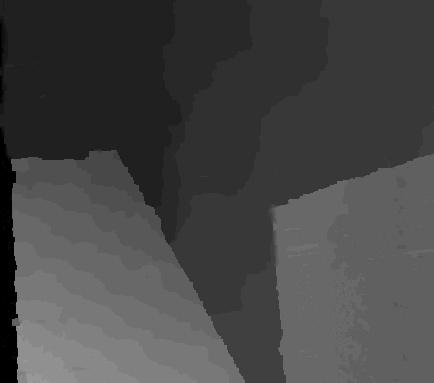
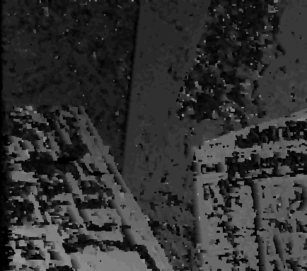
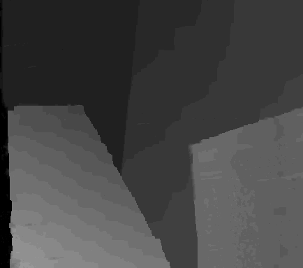
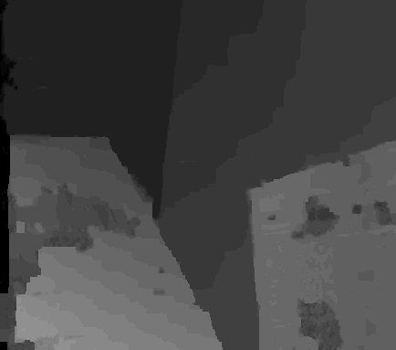
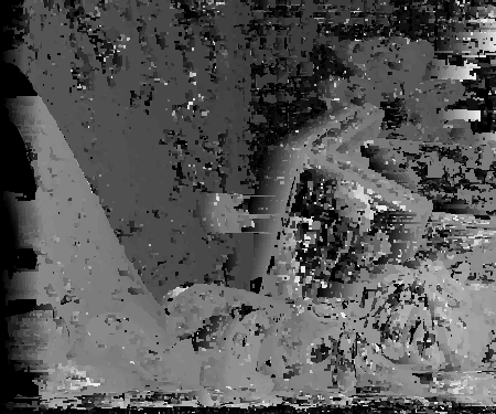
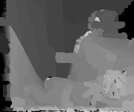
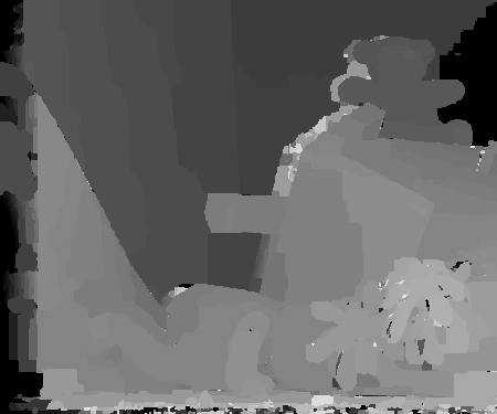
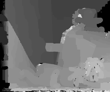
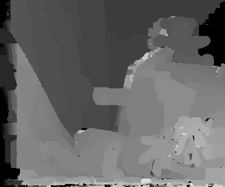
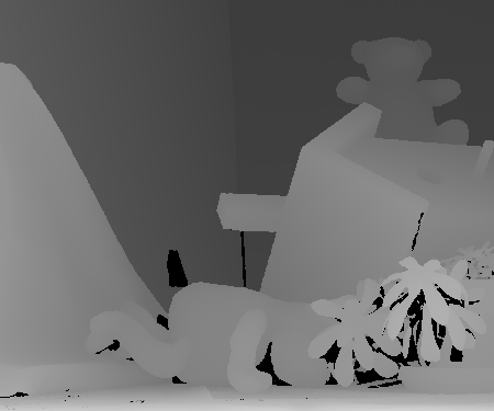
Figure 47: Stereo: Note how our multiscale framework drastically improves ICM results. visible improvement for $\alpha\beta$-swap can also be seen in the middle row (Venus). Numerical results for these examples are shown in Table 10.

	ICM		Swap		Expand
	Ours	single scale	Ours	single scale	Ours	single scale
House	$100.5\%$	$111.3\%$	$100.4\%$	$100.9\%$	$102.3\%$	$103.4\%$
Penguin	$106.9\%$	$132.9\%$	$104.6\%$	$111.3\%$	$104.0\%$	$103.7\%$

Table 11: Denoising and inpainting: Showing percent of achieved energy value relative to the lower bound (closer to $100\%$ is better). Visual results for these experiments are in Fig. 48. Energies from Szeliski et al. (2008).

Input	ICM		Swap		Expand
	Ours	Single scale	Ours	Single scale	Ours	Single scale

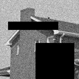
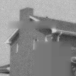
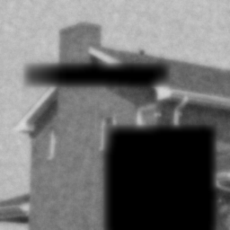
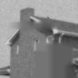
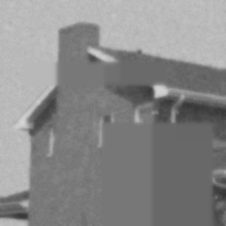
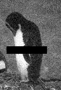
Figure 48: Denoising and inpainting: Single scale ICM is unable to cope with inpainting: performing local steps it is unable to propagate information far enough to fill the missing regions in the images. On the other hand, our multiscale framework allows ICM to perform large steps at coarse scales and successfully fill the gaps. Numerical results for these examples are shown in Table 11.

40.5 Comparing variable correlation estimation methods

As explained in Sec. 38 the correlations between the variables are the most crucial component in constructing an effective multiscale scheme. In this experiment we compare our energy-aware correlation measure (Sec. 38.1) to three methods proposed by Kim et al. (2011): “unary-diff”, “min-unary-diff” and “mean-compat”. These methods estimate the correlations based either on the unary term or the pair-wise term, but not both. We also compare to an energy-agnostic measure, that is $c_{ij}=1$ $\forall i,j$, this method underlies Felzenszwalb and Huttenlocher (2006). We use ICM within our framework to evaluate the influence these methods have on the resulting multiscale performance for four representative energies.

Fig. 49 shows percent of lower bound for the different energies. Our measure consistently outperforms all other methods, and successfully balances between the influence of the unary and the pair-wise terms.

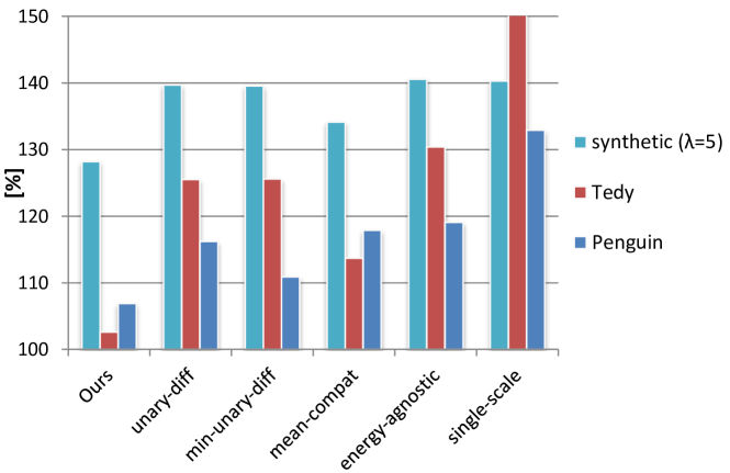
Figure 49: Comparing correlation measures: Graphs showing percent of lower bound (closer to $100\%$ is better) for different methods of computing variable-correlations. Some of the bars are cropped at $\sim 150\%$. Our energy-aware measure consistently outperforms all other methods.

40.6 Coarsening labels

$\alpha\beta$-swap does not scale gracefully with the number of labels. Coarsening an energy in the labels domain (i.e., same number of variables, fewer labels) proves to significantly improve performance of $\alpha\beta$-swap, as shown in Table 12. For these examples constructing the energy pyramid took only milliseconds, due to the “closed form” formula for estimating label correlations.

Our principled framework for coarsening labels improves $\alpha\beta$-swap performance for these energies.

Energy	#labels	#labels	Ours	single
	(finest)	(coarsest)		scale
Penguin	256	67	$103.6\%$	$111.3\%$
(denoising)			$128$ [sec]	$253$ [sec]
Venus	20	4	$106.0\%$	$128.7\%$
(stereo)			$100$ [sec]	$130$ [sec]

Table 12: Coarsening labels ($\alpha\beta$-swap): Working coarse-to-fine in the labels domain. We use 5 scales with coarsening rate of $\sim 0.7$. Number of variables is unchanged. Table shows percent of achieved energy value relative to the lower bound (closer to $100\%$ is better), and running times.

41 Conclusion

This work presents a unified multiscale framework for discrete energy minimization that allows for efficient and direct exploration of the multiscale landscape of the energy. We propose two paths to expose the multiscale landscape of the energy: one in which coarser scales involve fewer and coarser variables, and another in which the coarser levels involve fewer labels. We also propose adaptive methods for energy-aware interpolation between the scales. Our multiscale framework significantly improves optimization results for challenging energies.

Our framework provides the mathematical formulation that “bridges the gap” and relates multiscale discrete optimization and algebraic multiscale methods used in PDE solvers (e.g., Brandt (1986)). This connection allows for methods and practices developed for numerical solvers to be applied in multiscale discrete optimization as well.

Appendix

Appendix 8.A Derivation of eq. (50)

In this work we consider discrete pair-wise minimization problems of the form:

$E\left(L\right)=\sum_{i\in\mbox{$\mathcal{V}$}}\psi_{i}\left(l_{i}\right)+\sum_{\left(i,j\right)\in\mbox{$\mathcal{E}$}}w_{ij}\cdot\psi\left(l_{i},l_{j}\right)$ (49)

Using the following parameterizations: $D\in\mathbb{R}^{n\times l}$ s.t. $D_{i,\alpha}\mbox{$\stackrel{{\scriptstyle\mbox{\tiny{def}}}}{{=}}$}\psi_{i}(\alpha)$, and $V\in\mathbb{R}^{l\times l}$ s.t. $V_{\alpha,\beta}\mbox{$\stackrel{{\scriptstyle\mbox{\tiny{def}}}}{{=}}$}\psi\left(\alpha,\beta\right)$ we claim that (49) is equivalent to:

$E\left(U\right)=Tr\left(DU^{T}+WUVU^{T}\right)$ (50)

s.t. $U\in\left\{0,1\right\}^{n\times l},\ \sum_{\alpha=1}^{l}U_{i\alpha}=1$ (51)

Assuming both $V$ and $W$ are symmetric. Looking at the different components in (50):

$$\left[VU^{T}\right]_{\alpha j}=\sum_{\beta}V_{\alpha\beta}U_{j\beta}$$

$$\left[UVU^{T}\right]_{ij} = \sum_{\alpha}U_{i\alpha}\left[VU^{T}\right]_{\alpha j}$$

$$= \sum_{\alpha}U_{i\alpha}\sum_{\beta}V_{\alpha\beta}U_{j\beta}$$

$$= \sum_{\alpha\beta}V_{\alpha\beta}U_{i\alpha}U_{j\beta}$$

$$= \sum_{\alpha\beta}\psi\left(\alpha,\beta\right)U_{i\alpha}U_{j\beta}$$

$$= \psi\left(l_{i},l_{j}\right)$$

Looking at the trace of the second term:

$$Tr\left(WUVU^{T}\right) = \sum_{i}\left[WUVU^{T}\right]_{ii}$$ (56)

$$= \sum_{i}\sum_{j}w_{ij}\left[UVU^{T}\right]_{ji}$$

$$= \sum_{i}\sum_{j}w_{ij}\psi\left(l_{j},l_{i}\right)$$

$$= \sum_{ij}w_{ij}\psi\left(l_{i},l_{j}\right)$$

As for the unary term:

$$Tr\left(DU^{T}\right) = \sum_{i}\left[DU^{T}\right]_{ii}$$ (57)

$$= \sum_{i}\sum_{\alpha}D_{i\alpha}U_{i\alpha}$$

$$= \sum_{i}\sum_{\alpha}\psi_{i}\left(\alpha\right)U_{i\alpha}$$

$$= \sum_{i}\psi_{i}\left(l_{i}\right)$$

Putting (57) and (56) together we get:

$$Tr\left(DU^{T}+WUVU^{T}\right) = Tr\left(DU^{T}\right)+Tr\left(WUVU^{T}\right)$$

$$= \sum_{i}\psi_{i}\left(l_{i}\right)+\sum_{ij}w_{ij}\psi\left(l_{i},l_{j}\right)\quad\square$$

Note that the diagonal of $W$ is assumed to be zero: this is a reasonable assumption as $w_{ii}$ represents an interaction of variable $i$ with itself. This type of interaction is well represented by the unary term $D_{i}$. When coarsening the energy it may happen that $W^{c}$ will no longer have zeros on the diagonal. This case may arise when a single coarse variable represents neighboring fine scale variables. In that case the fine scale pair-wise interaction should be absorbed into the coarse scale unary term. It is easy to see that the term $w_{ii}V_{\alpha\alpha}$ should be added to the unary term $D_{i\alpha}$, whenever $W$ has non zeros on the diagonal. After this rectification, the non-zeros entries on the diagonal of $W$ can be set to zero.

Appendix 8.B More General Energy Functions

This chapter (8) has focused on the construction of an energy pyramid for energies of the form (49). However, this form does not cover all possible pair-wise energies. We have used this slightly restricted form throughout the paper since it emphasizes the simplicity of the algebraic derivation of our multiscale framework. Nevertheless, our multiscale framework can be as easily applied to more general energies.

8.B.1 Pair-wise

A general from for pair-wise energy over a graph $\mbox{$\mathcal{G}$}=\left(\mbox{$\mathcal{V}$},\mbox{$\mathcal{E}$}\right)$ can be written as

$$E\left(L\right)=\sum_{i\in\mbox{$\mathcal{V}$}}\varphi_{i}\left(l_{i}\right)+\sum_{\left(i,j\right)\in\mbox{$\mathcal{E}$}}\varphi_{ij}\left(l_{i},l_{j}\right)$$ (58)

In this more general form, the pair-wise term can be entirely different for each pair: $\varphi_{ij}\left(l_{i},l_{j}\right)$. This is in contrast to the energy (49) where the pair-wise terms differ only by the scaling factor $w_{ij}$ of a single fixed term $\varphi\left(l_{i},l_{j}\right)$. The Photomontage energies of (Szeliski et al., 2008, §4.2) are an example of such general pair-wise energies.

Instead of using a pair of matrices $V$ and $W$ to parameterize the pair-wise terms, we use a collection of matrices $\left\{V^{ij}\right\}_{ij\in\mbox{$\mathcal{E}$}}$ for the same purpose in the general settings. Each matrix $V^{ij}$ is of size $l\times l$ and is defined as $V^{ij}_{\alpha\beta}\mbox{$\stackrel{{\scriptstyle\mbox{\tiny{def}}}}{{=}}$}\varphi_{ij}\left(\alpha,\beta\right)$.

A general energy is now parameterized by $\left(n,l,D,\left\{V^{ij}\right\}_{ij\in\mbox{$\mathcal{E}$}}\right)$.

Coarsening variables: The computation of the interpolation matrix $P$ is unchanged. ICM can be applied to energies of the form (58) to estimate agreement between neighboring variables. These agreements are then used to compute the interpolation matrix $P$ (Sec. 38).

In order to write the coarsening of the pair-wise term we need to introduce some notations: Let $i,j$ be variables at the fine scale, and $I,J$ denote variables in the coarse scale. An entry, $P_{iI}$, in the interpolation matrix indicates how fine scale variable $i$ is affected by a coarse scale variable $I$. Given an interpolation matrix $P$ we can coarsen the energy by

$$D^{c} \stackrel{{\scriptstyle\mbox{\tiny{def}}}}{{=}} P^{T}D^{f}$$

$$\mbox{$V^{IJ}$}_{\alpha\beta} \stackrel{{\scriptstyle\mbox{\tiny{def}}}}{{=}} \sum_{ij\in\mbox{$\mathcal{E}$}^{f}}\mbox{$V^{ij}$}_{\alpha\beta}P_{iJ}P_{jJ}$$ (59)

The coarse graph, $\mbox{$\mathcal{E}$}^{c}$, is defined by all the non-zero pair-wise terms $V^{IJ}$. The coarser energy is now parameterized by

$$\left(n^{c},l,D^{c},\left\{\mbox{$V^{IJ}$}\right\}_{ij\in\mbox{$\mathcal{E}$}^{c}}\right)$$

Coarsening labels: In this case, the computation of the interpolation matrix $\hat{P}$ is not trivial, since we no longer have a single matrix $V$ to derive the agreements from. We leave this issue of deriving an efficient interpolation matrix for the general case for future work. However, given a matrix $\hat{P}$ the coarsening of labels can be done easily:

$$D^{\hat{c}} \stackrel{{\scriptstyle\mbox{\tiny{def}}}}{{=}} D^{\hat{f}}\hat{P}$$

$$\mbox{$V^{ij}$}^{\hat{c}} \stackrel{{\scriptstyle\mbox{\tiny{def}}}}{{=}} \hat{P}^{T}\mbox{$V^{ij}$}^{\hat{f}}\hat{P}\;\;\forall ij\in\mbox{$\mathcal{E}$}$$ (60)

yielding a coarser energy parameterized by

$$\left(n,l^{c},D^{\hat{c}},\left\{\mbox{$V^{ij}$}^{\hat{c}}\right\}_{ij\in\mbox{$\mathcal{E}$}}\right)$$

with the same number of variables, $n$, but fewer labels $l^{c}<l^{f}$.

It is fairly straight forward to see that the energy (49) is a special case of the more general form (58) and so the coarsening of variables and labels of Eq. (53) and (54) can be seen as special cases of Eq. (59) and (60) resp.

8.B.2 High-order energies

Discrete energies may involve terms that are beyond pair-wise: that is, describe interaction between sets of variables. These energies are often referred to as high-order energies. Examples of such energies can be found in e.g., Kohli et al. (2009); Rother et al. (2009).

A high order energy is defined over a hyper-graph $\left(\mbox{$\mathcal{V}$},\mbox{$\mathcal{S}$}\right)$ where the hyper-edges are subsets of variables $s\in\mbox{$\mathcal{S}$}$ s.t. $s\subseteq\mbox{$\mathcal{V}$}$.

$$E\left(L\right)=\sum_{i\in\mbox{$\mathcal{V}$}}\varphi_{i}\left(l_{i}\right)+\sum_{s\in\mbox{$\mathcal{S}$}}\varphi_{s}\left(\left\{l_{i}\left|i\in s\right.\right\}\right)$$ (61)

Where the high-order terms $\varphi_{s}$ are $\left|s\right|$-way discrete functions:

$$\varphi_{s}:\left\{1,\ldots,l\right\}^{\mbox{$\left|s\right|$}}\rightarrow\mathbb{R}$$ (62)

A high-order energy of the form (61) can be parameterized using tensors. Each high-order term, $\varphi_{s}$, is parameterized by a $\left|s\right|$-order tensor

$$V^{s}_{\alpha,\beta,\ldots,\zeta}\mbox{$\stackrel{{\scriptstyle\mbox{\tiny{def}}}}{{=}}$}\varphi_{s}\left(l_{i}=\alpha,l_{j}=\beta,\ldots,l_{m}=\zeta\left|s=\left\{i,j,\ldots,m\right\}\right.\right)$$ (63)

A high-order energy (61) is now parameterized by $\left(n,l,D,\left\{V^{s}\right\}_{s\in\mbox{$\mathcal{S}$}}\right)$.

Coarsening variables: The computation of the interpolation matrix $P$ is unchanged. ICM can be applied to energies of the form (61) to estimate agreement between neighboring variables. These agreements are then used to compute the interpolation matrix $P$ (Sec. 38).

Given an interpolation matrix $P$ we can coarsen the energy by

$$D^{c} \stackrel{{\scriptstyle\mbox{\tiny{def}}}}{{=}} P^{T}D^{f}$$

$$V^{S=\left\{I,J,\ldots,M\right\}} \stackrel{{\scriptstyle\mbox{\tiny{def}}}}{{=}} P_{iI}\cdot P_{jJ}\cdot\ldots V^{\left\{s=i,j,\ldots,m\right\}}\;\;\forall s\in\mbox{$\mathcal{S}$}^{f}$$ (64)

For all coarse variables $I,J,\ldots,M$ with non-zero entry $P_{iI},P_{jJ},\ldots$. These non-zeros interactions in $P$ defines the coarse scale hyper-edges in $\mbox{$\mathcal{S}$}^{c}$. Note that when two (or more) fine-scale variable $i,j,\ldots$ are represented by the same coarse variable $I$, then the size of $S$ (the coarse scale hyper-edge) is reduced relative to the size of $s$ (the fine scale hyper-edge).

Coarsening labels: In this case, the computation of the interpolation matrix $\hat{P}$ is not trivial, since we no longer have a clear representation of the interactions between the different labels. We leave this issue of deriving an efficient interpolation matrix for the general case for future work. However, given a matrix $\hat{P}$ the coarsening of labels can be done easily. Using $\boldsymbol{\alpha},\boldsymbol{\beta}$ to denote coarse scale labels

$$D^{\hat{c}} \stackrel{{\scriptstyle\mbox{\tiny{def}}}}{{=}} D^{\hat{f}}\hat{P}$$

$$\mbox{$V^{s}$}^{\hat{c}}_{\boldsymbol{\alpha},\boldsymbol{\beta},\ldots} \stackrel{{\scriptstyle\mbox{\tiny{def}}}}{{=}} \sum_{\alpha,\beta,\ldots}\mbox{$V^{s}$}^{\hat{f}}_{\alpha,\beta,\ldots}\hat{P}_{\alpha\boldsymbol{\alpha}}\cdot\hat{P}_{\beta\boldsymbol{\beta}}\cdot\ldots$$ (65)

yielding a coarser energy parameterized by

$$\left(n,l^{c},D^{\hat{c}},\left\{\mbox{$V^{s}$}^{\hat{c}}\right\}_{s\in\mbox{$\mathcal{S}$}}\right)$$

with the same number of variables, $n$, but fewer labels $l^{c}<l^{f}$.

Part IV Discussion

In this work I motivated the use of challenging discrete energies, beyond semi-metric, for different tasks in computer vision. I conclude that despite the computational challenges posed by stepping away form the well studied smoothness-encouraging energies, the gain in terms of expressiveness and quality of solution is worth while. For some applications these energies describe better the underlying process and therefore better suited for modeling. Moreover, practical algorithms and approaches were proposed in this work to cope with the resulting challenging optimization tasks.

Considering the task of unsupervised clustering as an example, using the arbitrary Potts energy of the Correlation Clustering functional allows not only to model the partition of the data into different clusters, but also to recover the underlying number of clusters. This recovery of the number of cluster is an issue usually evaded by many clustering algorithms that assume this information is somehow given to them as an input. This thesis showed how the challenging optimization of the CC functional lies at the core of several diverse applications, such as: sketching the common, unsupervised face identification and interactive segmentation.

Focusing on the CC optimization example, this work also proposed several practical approximation algorithms. The CC functional was casted as a special case of an arbitrary Potts energy minimization. This discrete formulation of the functional allows to adapt and utilize known methods for discrete optimization resulting with CC optimization algorithms capable of handling large number of variables (two orders of magnitude more than existing methods).

Another example of challenging arbitrary energy is the task of 3D shape reconstruction. The problem of 3D reconstruction from two images with common lighting conditions and known object motion with respect to static camera is discretized to form a challenging energy. This energy emerges from the induced integrality constraints on the recovered surface. It is defined over a very large label space (a few thousand of labels). Despite the challenging pair-wise terms and the large label space successful approximation scheme was proposed and adapted for this task.

When it comes to learning the parameters of discrete energies for various tasks in computer vision, it so happens that the underlying data may be better explained by contrast enhancing terms, as in the Chinese characters and the body parts. In fact when the learning procedure is not restricted it may prefer contrast-enhancing functions as better depictions for the underlying statistical behavior of the training set. Therefore, restricting the learned model to only submodular or semi-metric energies might severely compromise its ability to generalize to novel exemplars.

Coping with the optimization of the resulting challenging energies is a difficult task. Yet, this work proposes several methods that provide good empirical approximations for a variety of practical energies. Our unified discrete multiscale framework succeeds in providing good approximations, in practice, for a variety of challenging energies. Our multiscale framework exploits the underlying multiscale landscape of the given energy and exposes it to allow for an efficient and effective coarse-to-fine optimization process. Formulating the coarsening procedure in a clear algebraic formulation allows us to propose two paths to expose the multiscale landscape of the energy: one in which coarser scales involve fewer and coarser variables, and another in which the coarser levels involve fewer labels. We also propose adaptive methods for energy-aware interpolation between the scales. This approach exploits the underlying multiscale landscape of the given energy and exposes it to allow for an efficient and effective coarse-to-fine optimization process. Our framework provides the mathematical formulation that “bridges the gap” and relates multiscale discrete optimization and algebraic multiscale methods used in PDE solvers (e.g., Brandt (1986)). This connection allows for methods and practices developed for numerical solvers to be applied in multiscale discrete optimization as well.

References

- Alpert et al. (2007) S. Alpert, M. Galun, R. Basri, and A. Brandt. Image segmentation by probabilistic bottom-up aggregation and cue integration. In CVPR, 2007.
- Anguelov et al. (2005) D. Anguelov, B. Taskar, V. Chatalbashev, D. Koller, D. Gupta, G. Heitz, and A. Ng. Discriminative learning of Markov random fields for segmentation of 3D scan data. In CVPR, 2005.
- Bagon and Galun (2011) S. Bagon and M. Galun. Large scale correlation clustering optimization. arXiv, 2011.
- Bagon and Galun (2012) S. Bagon and M. Galun. A multiscale framework for challenging discrete optimization. In NIPS workshop on optimization for machine learning, 2012.
- Bagon et al. (2008) S. Bagon, O. Boiman, and M. Irani. What is a good image segment? a unified approach to segment extraction. In ECCV, 2008.
- Bagon et al. (2010) S. Bagon, O. Brostovsky, M. Galun, and M. Irani. Detecting and sketching the common. In CVPR, 2010.
- Bagon (2012) S. Bagon. Boundary driven interactive segmentation. In ICISA, 2012.
- Baker et al. (2007) S. Baker, D. Scharstein, J. P. Lewis, S. Roth, M. J. Black, and R. Szeliski. A database and evaluation methodology for optical flow. In ICCV, 2007.
- Bansal et al. (2004) N. Bansal, A. Blum, and S. Chawla. Correlation clustering. Machine Learning, 56(1):89–113, 2004.
- Basri and Frolova (2008) R. Basri and D. Frolova. A two-frame theory of motion, lighting and shape. In CVPR, 2008.
- Basri and Jacobs (2003) R. Basri and D. Jacobs. Lambertian reflectance and linear subspaces. PAMI, 25(2):218–233, February 2003.
- Batra et al. (2008) D. Batra, R. Sukthankar, and T. Chen. Learning class-specific affinities for image labelling. In CVPR, 2008.
- Besag (1977) J. Besag. Efficiency of pseudolikelihood estimation for simple Gaussian fields. Biometrica, (64):616–618, 1977.
- Besag (1986) J. Besag. On the statistical analysis of dirty pictures. Journal of the Royal Statistical Society. Series B (Methodological), 1986.
- Black et al. (2000) M. J. Black, D. J. Fleet, and Y. Yacoob. Robustly estimating changes in image appearance. CVIU, 78(1):8–31, 2000.
- Blake et al. (2004) A. Blake, C. Rother, M. Brown, P. Perez, and P. Torr. Interactive image segmentation using an adaptive GMMRF model. In ECCV, 2004.
- Blake et al. (2011) A. Blake, P. Kohli, and C. Rother. Markov Random Fields for Vision and Image Processing. MIT Press, 2011.
- Bleyer et al. (2010) M. Bleyer, C. Rother, and P. Kohli. Surface stereo with soft segmentation. In CVPR, 2010.
- Boiman and Irani (2007) O. Boiman and M. Irani. Similarity by composition. In NIPS, 2007.
- Boykov et al. (2001) Y. Boykov, O. Veksler, and R. Zabih. Fast approximate energy minimization via graph cuts. PAMI, 2001.
- Brandt (1986) A. Brandt. Algebraic multigrid theory: The symmetric case. Applied Mathematics and Computation, 1986.
- Breiman (2001) L. Breiman. Random forests. Machine Learning, 45(1), 2001.
- Burkard (2007) R. Burkard. Monge properties, discrete convexity and applications. European journal of operational research, 2007.
- Burt and Adelson (1983) P. Burt and E. Adelson. The laplacian pyramid as a compact image code. IEEE Transac. on Commun., 1983.
- Carceroni and Kutulakos (2001) R. Carceroni and K. Kutulakos. Multi-View scene capture by surfel sampling: From video streams to Non-Rigid 3D motion, shape & reflectance. In ICCV, pages 60–67, June 2001.
- Cechlárová and Szabó (1990) K. Cechlárová and P. Szabó. On the Monge property of matrices. Discrete Mathematics, 1990.
- Chen et al. (2009) C.-P. Chen, C.-S. Chen, and Y.-P. Hung. Pixel-based correspondence and shape reconstruction for moving objects. In Workshop on Color and Reflectance in Imaging and Computer Vision, 2009.
- Chen (2011) T. Chen. Chinese Calligraphy. Cambridge University Press, 2011.
- Cho et al. (2010) T. S. Cho, N. Joshi, C. L. Zitnick, S. B. Kang, R. Szeliski, and W. T. Freeman. A content-aware image prior. In CVPR, 2010.
- Chum and Zisserman (2007) O. Chum and A. Zisserman. An exemplar model for learning object classes. In CVPR, 2007.
- Chum et al. (2009) O. Chum, M. Perdoch, and J. Matas. Geometric min-hashing: Finding a (thick) needle in a haystack. In CVPR, 2009.
- Cormen et al. (2001) T. Cormen, C. Leiserson, R. Rivest, and C. Stein. Introduction to algorithms. The MIT press, 2001.
- Crandall et al. (2011) D. Crandall, A. Owens, N. Snavely, and D. P. Huttenlocher. Discrete-continuous optimization for large-scale structure from motion. In CVPR, 2011.
- Cryer et al. (1995) J. Cryer, P. Tsai, and M. Shah. Integration of shape from shading and stereo. Pattern Recognition, 28(7):1033–1043, July 1995.
- Demaine and Immorlica (2003) E. Demaine and N. Immorlica. Correlation clustering with partial information. Approximation, Randomization, and Combinatorial Optimization. Algorithms and Techniques, pages 71–80, 2003.
- Elsner and Schudy (2009) M. Elsner and W. Schudy. Bounding and comparing methods for correlation clustering beyond ILP. In ILP NLP, 2009.
- Felzenszwalb and Huttenlocher (2006) P. Felzenszwalb and D. Huttenlocher. Efficient belief propagation for early vision. IJCV, 2006.
- Ferrari et al. (2006) V. Ferrari, T. Tuytelaars, and L. Van Gool. Object detection by contour segment networks. In ECCV, 2006.
- Ferrari et al. (2009) V. Ferrari, F. Jurie, , and C. Schmid. From images to shape models for object detection. IJCV, 2009.
- Fua and Leclerc (1995) P. Fua and Y. Leclerc. Object-centered surface reconstruction: Combining multi-image stereo and shading. IJCV, 16:35–56, September 1995.
- Geman and Geman (1984) S. Geman and D. Geman. Stochastic relaxation, Gibbs distributions, and the Bayesian restoration of images. PAMI, 6:721–741, 1984.
- Geurts et al. (2006) P. Geurts, D. Ernst, and L. Wehenkel. Extremely randomized trees. Machine Learning, 63(1), 2006.
- Glasner et al. (2011) D. Glasner, S. N. Vitaladevuni, and R. Basri. Contour-based joint clustering of multiple segmentations. In CVPR, 2011.
- Glesner and Koller (1995) S. Glesner and D. Koller. Constructing flexible dynamic belief networks from first-order probabilistic knowledge bases. In ECSQARU, 1995.
- Gould et al. (2009) S. Gould, R. Fulton, and D. Koller. Decomposing a scene into geometric and semantically consistent regions. In ICCV, 2009.
- Greig et al. (1989) D. Greig, B. Porteous, and A. Seheult. Exact maximum a posteriori estimation for binary images. Journal of the Royal Statistical Society. Series B (Methodological), 1989.
- Guillaumin et al. (2009) M. Guillaumin, J. Verbeek, and C. Schmid. Is that you? Metric Learning Approaches for Face Identification. In ICCV, 2009.
- Guillaumin et al. (2010) M. Guillaumin, J. Verbeek, and C. Schmid. Multiple instance metric learning from automatically labeled bags of faces. In ECCV, 2010.
- Hammer et al. (1984) P. Hammer, P. Hansen, and B. Simeone. Roof duality, complementation and persistency in quadratic 0–1 optimization. Mathematical Programming, 1984.
- Haussecker and Fleet (2001) H. W. Haussecker and D. J. Fleet. Computing optical flow with physical models of brightness variation. PAMI, 23(6):661–673, June 2001.
- He et al. (2004) X. He, R. S. Zemel, and M. Á. Carreira-Perpiñán. Multiscale conditional random fields for image labeling. In CVPR, 2004.
- Horn and Brooks (1989) B. Horn and M. Brooks. Shape from Shading. MIT Press, 1989.
- Horn and Schunk (1981) B. K. P. Horn and B. Schunk. Determining optical flow. Artificial Intelligence, 17:185–203, 1981.
- Hörster et al. (2008) E. Hörster, T. Greif, R. Lienhart, and M. Slaney. Comparing local feature descriptors in plsa-based image models. In DAGM, 2008.
- Isack and Boykov (2011) H. Isack and Y. Boykov. Energy-based geometric multi-model fitting. IJCV, 2011.
- Ishikawa (2003) H. Ishikawa. Exact optimization for markov random fields with convex priors. PAMI, 2003.
- Jin et al. (2008) H. Jin, D. Cremers, D. Wang, A. Yezzi, E. Prados, and S. Soatto. 3-D reconstruction of shaded objects from multiple images under unknown illumination. IJCV, 2008.
- Joshi and Kriegman (2007) N. Joshi and D. Kriegman. Shape from varying illumination and viewpoint. In ICCV, 2007.
- Karlinsky et al. (2008) L. Karlinsky, M. Dinerstein, D. Levi, and S. Ullman. Unsupervised classification and part localization by consistency amplification. In ECCV, 2008.
- Kasinski et al. (2008) A. Kasinski, A. Florek, and A. Schmidt. The PUT face database. Image Processing and Communications. v13, 2008.
- Kim et al. (2011) T. Kim, S. Nowozin, P. Kohli, and C. Yoo. Variable grouping for energy minimization. In CVPR, 2011.
- Kirkpatrick et al. (1983) S. Kirkpatrick, C. Gelatt Jr, and M. Vecchi. Optimization by simulated annealing. science, 1983.
- Kohli et al. (2008) P. Kohli, L. Ladicky, and P. Torr. Robust higher order potentials for enforcing label consistency. In CVPR, 2008.
- Kohli et al. (2009) P. Kohli, L. Ladický, and P. H. Torr. Robust higher order potentials for enforcing label consistency. IJCV, 2009.
- Koller and Friedman (2009) D. Koller and N. Friedman. Probabilistic Graphical Models: Principles and Techniques. MIT Press, 2009.
- Kolmogorov and Boykov (2005) V. Kolmogorov and Y. Boykov. What metrics can be approximated by geo-cuts, or global optimization of length/area and flux. In ICCV, 2005.
- Kolmogorov and Rother (2007) V. Kolmogorov and C. Rother. Minimizing nonsubmodular functions with graph cuts-a review. PAMI, 2007.
- Kolmogorov and Wainwright (2005) V. Kolmogorov and M. Wainwright. On the optimality of tree-reweighted max-product message passing. In Uncertainty in Artificial Intelligence, 2005.
- Kolmogorov and Zabih (2004) V. Kolmogorov and R. Zabih. What energy functions can be minimized via graph cuts? PAMI, 26(2):147–159, 2004.
- Kolmogorov (2006) V. Kolmogorov. Convergent tree-reweighted message passing for energy minimization. PAMI, 2006.
- Komodakis and Tziritas (2007) N. Komodakis and G. Tziritas. Approximate labeling via graph cuts based on linear programming. IEEE Trans. Pattern Anal. Mach. Intell, 29(8):1436–1453, 2007.
- Komodakis et al. (2011) N. Komodakis, N. Paragios, and G. Tziritas. MRF energy minimization and beyond via dual decomposition. PAMI, 2011.
- Komodakis (2010) N. Komodakis. Towards more efficient and effective LP-based algorithms for MRF optimization. In ECCV, 2010.
- Kumar et al. (2005) S. Kumar, J. August, and M. Hebert. Exploiting inference for approximate parameter learning in discriminative fields: An empirical study. In EMMCVPR, 2005.
- Lafferty et al. (2001) J. Lafferty, A. McCallum, and F. Pereira. Conditional random fields: Probabilistic models for segmenting and labeling sequence data. In ICML, 2001.
- Lee and Grauman (2009) Y. J. Lee and K. Grauman. Shape discovery from unlabeled image collections. In CVPR, 2009.
- Lee et al. (2009) H. Lee, R. Grosse, R. Ranganath, and A. Y. Ng. Convolutional deep belief networks for scalable unsupervised learning of hierarchical representations. In ICML, 2009.
- Lempitsky et al. (2007) V. Lempitsky, C. Rother, and A. Blake. Logcut-efficient graph cut optimization for markov random fields. In ICCV, 2007.
- Lempitsky et al. (2010) V. Lempitsky, C. Rother, S. Roth, and A. Blake. Fusion moves for markov random field optimization. PAMI, 2010.
- Levin et al. (2008) A. Levin, R. Acha, and D. Lischinski. Spectral matting. PAMI, 30(10):1699–1712, 2008.
- Li (1995) S. Z. Li. Markov Random Field Modeling in Computer Vision. Springer, 1995.
- Livne and Brandt (2011) O. E. Livne and A. Brandt. Lean Algebraic Multigrid (LAMG): Fast Graph Laplacian Linear Solver. arXiv:1108.1310v1, 2011.
- Lovász (1983) L. Lovász. Submodular functions and convexity. Mathematical programming: the state of the art, 1983.
- Lucas and Kanade (1981) B. Lucas and T. Kanade. An iterative image registration technique with an application to stereo vision. In International joint conference on artificial intelligence, 1981.
- Maire et al. (2008) M. Maire, P. Arbelaez, C. Fowlkes, and J. Malik. Using contours to detect and localize junctions in natural images. In CVPR, 2008.
- Maki et al. (2002) A. Maki, M. Watanabe, and C. Wiles. Geotensity: Combining motion and lighting for 3d surface reconstruction. IJCV, 48(2):75–90, July 2002.
- Monge (1781) G. Monge. Me’moire sur la the’orie des de’blais et des remblais. De l’Imprimerie Royale, 1781.
- Moses and Shimshoni (2006) Y. Moses and I. Shimshoni. 3D shape recovery of smooth surfaces: Dropping the fixed viewpoint assumption. In ACCV, 2006.
- Mukawa (1990) N. Mukawa. Estimation of shape, reflection coefficients and illumination direction from image sequences. In ICCV:507-512, 1990.
- Mukherjee et al. (2009) L. Mukherjee, V. Singh, and C. Dyer. Half-integrality based algorithms for cosegmentation of images. In CVPR, 2009.
- Negahdaripour (1998) S. Negahdaripour. Revised definition of optical flow: Integration of radiometric and geometric cues for dynamic scene analysis. PAMI, 20(9):961–979, September 1998.
- Nguyen et al. (2009) M. H. Nguyen, L. Torresani, F. de la Torre, and C. Rother. Weakly supervised discriminative localization and classification: a joint learning process. In ICCV, 2009.
- Nowozin and Jegelka (2009) S. Nowozin and S. Jegelka. Solution stability in linear programming relaxations: Graph partitioning and unsupervised learning. In ICML, 2009.
- Nowozin and Lampert (2009) S. Nowozin and C. H. Lampert. Global connectivity potentials for random field models. In CVPR, 2009.
- Nowozin and Lampert (2011) S. Nowozin and C. Lampert. Structured learning and prediction in computer vision. Now Publishers, 2011.
- Nowozin et al. (2011) S. Nowozin, C. Rother, S. Bagon, T. Sharp, B. Yao, and P. Kohli. Decision tree fields. In ICCV, 2011.
- Payet and Todorovic (2010) N. Payet and S. Todorovic. (RF)2 – random forest random field. In NIPS, 2010.
- Pearl (1988) J. Pearl. Probabilistic reasoning in intelligent systems: networks of plausible inference. Morgan Kaufmann, 1988.
- Prasad et al. (2006) M. Prasad, A. Zisserman, A. W. Fitzgibbon, M. P. Kumar, and P. H. S. Torr. Learning class-specific edges for object detection and segmentation. In ICVGIP, 2006.
- Pritch et al. (2009) Y. Pritch, E. Kav-Venaki, and S. Peleg. Shift-map image editing. In ICCV, 2009.
- Rangarajan (2000) A. Rangarajan. Self-annealing and self-annihilation: unifying deterministic annealing and relaxation labeling. Pattern Recognition, 2000.
- Rennie and Dobson (1969) B. Rennie and A. Dobson. On stirling numbers of the second kind. Journal of Combinatorial Theory, 1969.
- Ron et al. (2011) D. Ron, I. Safro, and A. Brandt. Relaxation-based coarsening and multiscale graph organization. SIAM Multi Scale Modeling and Simulation, 2011.
- Roth and Black (2007) S. Roth and M. J. Black. Steerable random fields. In ICCV, 2007.
- Roth and Black (2009) S. Roth and M. J. Black. Fields of experts. IJCV, 82(2):205–229, 2009.
- Rother et al. (2004a) C. Rother, V. Kolmogorov, and A. Blake. ”GrabCut”: interactive foreground extraction using iterated graph cuts. ACM Transactions on Graphics (TOG), 23(3):309–314, 2004.
- Rother et al. (2004b) C. Rother, V. Kolmogorov, T. Minka, and A. Blake. Cosegmentation of image pairs by histogram matching-incorporating a global constraint into MRFs. In CVPR, 2004.
- Rother et al. (2007) C. Rother, V. Kolmogorov, V. Lempitsky, and M. Szummer. Optimizing binary MRFs via extended roof duality. In CVPR, 2007.
- Rother et al. (2009) C. Rother, P. Kohli, W. Feng, and J. Jia. Minimizing sparse higher order energy functions of discrete variables. In CVPR, 2009.
- R.Ramamoorthi and P.Hanrahan (2001) R.Ramamoorthi and P.Hanrahan. On the relationship between radiance and irradiance: Determining the illumination from images of a convex lambertian object. JOSA A, pages 2448–2459, October 2001.
- Santner et al. (2011) J. Santner, T. Pock, and H. Bischof. Interactive multi-label segmentation. In ACCV, 2011.
- Schlesinger and Flach (2006) D. Schlesinger and B. Flach. Transforming an arbitrary minsum problem into a binary one. Technical report, TU, Fak. Informatik, 2006.
- Schnitzspan et al. (2010) P. Schnitzspan, S. Roth, and B. Schiele. Automatic discovery of meaningful object parts with latent CRFs. In CVPR, 2010.
- Sharp (2008) T. Sharp. Implementing decision trees and forests on a gpu. In ECCV, 2008.
- Shechtman and Irani (2007) E. Shechtman and M. Irani. Matching local self-similarities across images and videos. In CVPR, 2007.
- Shi and Malik (2000) J. Shi and J. Malik. Normalized cuts and image segmentation. IEEE Transactions on pattern analysis and machine intelligence, 22(8):888–905, 2000.
- Shotton et al. (2007) J. Shotton, J. Winn, C. Rother, and A. Criminisi. Textonboost for image understanding: Multi-class object recognition and segmentation by jointly modeling texture, layout, and context. IJCV, 81(1), 2007.
- Shotton et al. (2008) J. Shotton, M. Johnson, and R. Cipolla. Semantic texton forests for image categorization and segmentation. In CVPR, 2008.
- Shotton et al. (2011) J. Shotton, A. Fitzgibbon, M. Cook, T. Sharp, M. Finocchio, R. Moore, A. Kipman, and A. Blake. Real-time human pose recognition in parts from a single depth image. In CVPR, 2011.
- Simakov et al. (2003) D. Simakov, D. Frolova, and R. Basri. Dense shape reconstruction of a moving object under arbitrary, unknown lighting. In ICCV, pages 1202–1207, 2003.
- Snow et al. (2000) D. Snow, P. Viola, and R. Zabih. Exact voxel occupancy with graph cuts. In CVPR, 2000.
- Stein et al. (2008) A. Stein, T. Stepleton, and M. Hebert. Towards unsupervised whole-object segmentation: Combining automated matting with boundary detection. In CVPR, 2008.
- Sutton and McCallum (2007) C. Sutton and A. McCallum. An introduction to conditional random fields for relational learning. In Introduction to Statistical Relational Learning, chapter 4. 2007.
- Swendsen and Wang (1987) R. H. Swendsen and J.-S. Wang. Nonuniversal critical dynamics in MC simulations. Phys. Rev. Lett., 1987.
- Szeliski et al. (2008) R. Szeliski, R. Zabih, D. Scharstein, O. Veksler, V. Kolmogorov, A. Agarwala, M. Tappen, and C. Rother. A comparative study of energy minimization methods for markov random fields with smoothness-based priors. PAMI, 2008.
- Szummer et al. (2008) M. Szummer, P. Kohli, and D. Hoiem. Learning CRFs using graph cuts. In ECCV, 2008.
- Taskar et al. (2003) B. Taskar, C. Guestrin, and D. Koller. Max-margin markov networks. In NIPS, 2003.
- Taskar et al. (2005) B. Taskar, V. Chatalbashev, D. Koller, and C. Guestrin. Learning structured prediction models: a large margin approach. In ICML, 2005.
- Tsochantaridis et al. (2006) I. Tsochantaridis, T. Joachims, T. Hofmann, and Y. Altun. Large margin methods for structured and interdependent output variables. Journal of Machine Learning Research, 2006.
- Tu and Bai (2010) Z. Tu and X. Bai. Auto-context and its application to high-level vision tasks and 3d brain image segmentation. PAMI, 2010.
- Varga (1962) R. S. Varga. Matrix iterative analysis. Prentice-Hall, Englewood Cliffs, NJ, 1962.
- Vitaladevuni and Basri (2010) S. Vitaladevuni and R. Basri. Co-clustering of Image Segments Using Convex Optimization Applied to EM Neuronal Reconstruction. In CVPR, 2010.
- Vogiatzis et al. (2005) G. Vogiatzis, P. Torr, and R. Cipolla. Multi-view stereo via volumetric graph-cuts. In CVPR, 2005.
- Wainwright and Jordan (2008) M. J. Wainwright and M. I. Jordan. Graphical models, exponential families, and variational inference. Foundations and Trends in Machine Learning, 1(1-2), 2008.
- Wainwright et al. (2005) M. Wainwright, T. Jaakkola, and A. Willsky. MAP estimation via agreement on trees: message-passing and linear programming. Information Theory, IEEE Transactions on, 2005.
- Weber et al. (2004) M. Weber, A. Blake, and R. Cipolla. Towards a complete dense geometric and photometric reconstruction under varying pose and illumination. IVC, 22(10):787–793, September 2004.
- Werner (2007) T. Werner. A linear programming approach to max-sum problem: A review. PAMI, 2007.
- Winn and Jojic (2005) J. Winn and N. Jojic. LOCUS: Learning object classes with unsupervised segmentation. In ICCV, 2005.
- Winn and Shotton (2006) J. M. Winn and J. Shotton. The layout consistent random field for recognizing and segmenting partially occluded objects. In CVPR, 2006.
- Woodham (1980) R. Woodham. Photometric method for determining surface orientation from multiple images. OptEng, 19(1):139–144, Jan. 1980.
- Wu et al. (2009) Y. N. Wu, Z. Si, H. Gong, and S.-C. Zhu. Learning active basis model for object detection and recognition. IJCV, 2009.
- Yu and Shi (2001) S. X. Yu and J. Shi. Understanding popout through repulsion. In CVPR, 2001.
- Zhang and Seitz (2005) L. Zhang and S. M. Seitz. Parameter estimation for MRF stereo. In CVPR, 2005.
- Zhang et al. (2003) L. Zhang, B. Curless, A. Hertzmann, and S. M. Seitz. Shape and motion under varying illumination: unifying multiview stereo, photometric stereo, and structure from motion. In ICCV, 2003.
- Zhu et al. (1997) C. Zhu, R. H. Byrd, P. Lu, and J. Nocedal. Algorithm 778: L-BFGS-B: Fortran subroutines for large-scale bound-constrained optimization. ACM Trans. Math. Softw, 23(4):550–560, 1997.
- Zhu et al. (2008) L. Zhu, C. Lin, H. Huang, Y. Chen, and A. Yuille. Unsupervised structure learning: hierarchical recursive composition, suspicious coincidence and competitive exclusion. In ECCV, 2008.