Measurement error in two-stage analyses, with application to air pollution epidemiology

Abstract

Public health researchers often estimate health effects of exposures (e.g., pollution, diet, lifestyle) that cannot be directly measured for study subjects. A common strategy in environmental epidemiology is to use a first-stage (exposure) model to estimate the exposure based on covariates and/or spatio-temporal proximity and to use predictions from the exposure model as the covariate of interest in the second-stage (health) model. This induces a complex form of measurement error. We propose an analytical framework and methodology that is robust to misspecification of the first-stage model and provides valid inference for the second-stage model parameter of interest.

We decompose the measurement error into components analogous to classical and Berkson error and characterize properties of the estimator in the second-stage model if the first-stage model predictions are plugged in without correction. Specifically, we derive conditions for compatibility between the first- and second-stage models that guarantee consistency (and have direct and important real-world design implications), and we derive an asymptotic estimate of finite-sample bias when the compatibility conditions are satisfied. We propose a methodology that (1) corrects for finite-sample bias and (2) correctly estimates standard errors. We demonstrate the utility of our methodology in simulations and an example from air pollution epidemiology.

1 Introduction

We consider measurement error that results from using predictions from a first-stage statistical model as the covariate of interest (the exposure) in a second-stage association study. Regardless of the exposure prediction model, there will be measurement error from the difference between predictions and the unmeasured true values. In contrast with standard measurement error models and the usual classification into classical and Berkson error, such predictions induce a complicated form of measurement error that is heteroscedastic and correlated across study subjects (Gryparis et al. 2009; Szpiro et al. 2011b). Our objectives are to characterize the effects of this error, to give guidelines for study design to minimize the impact, and to provide a correction method that reduces bias and gives valid confidence intervals.

In this section, we review the literature on measurement error correction for air pollution cohort studies and describe how our approach advances the state of the art (Section 1.1), comment on connections between our work and fundamental statistical issues concerning the interpretation of random effects models and the interplay between random vs. fixed covariate regression and misspecified mean models (Section 1.2), and outline the main sections of the paper (Section 1.3).

1.1 Measurement error

There has been extensive research on measurement error (Carroll et al. 2006), but the statistical literature has only recently begun to deal with the problem presented here. For spatial exposure contrasts, we have generalized the standard categories by decomposing the measurement error into a Berkson-like component from smoothing the exposure surface and a classical-like component from variability in estimating exposure model parameters (Gryparis et al. 2009; Szpiro et al. 2011b; Sheppard et al. 2011). We and others have also shown that the parametric bootstrap (or a computationally efficient approximation to the parametric bootstrap) can be used to correct for the effects of measurement error (Madsen et al. 2008; Lopiano et al. 2011; Szpiro et al. 2011b). However, validity of these results depends crucially on having a correctly specified exposure model. In practice such models are developed for predictive performance and often use predictors based on convenience, so we believe misspecification is ubiquitous. A distinguishing feature of our methodology in this paper is that it is robust to misspecification of the mean and/or variance in the exposure model and still provides valid second-stage inference.

We focus on two-stage analysis, as this is a common and practical approach when exposure is not directly measured. An alternative is a unified analysis in which the exposure model is a component of a joint model for the exposure and health data (e.g., Sinha et al. (2010) in nutritional epidemiology and Gryparis et al. (2009) in air pollution epidemiology), but this type of joint model has several difficulties. First, it presupposes that one has a correct (or at least nearly correct) exposure model; we argue that an exposure model can generally only capture a portion of the full exposure and should be treated in this light. Second, outlying second-stage data may influence estimation of the exposure model in unexpected ways, especially when the second-stage model is misspecified (noting at the same time that this feedback is an essential aspect of a coherent joint model and leads to increased efficiency). Third, the same exposure data are often used with multiple second-stage outcome data, and it is scientifically desirable to use the same predicted exposures across studies. Finally, exposure modeling can be computationally demanding, involving spatial and spatio-temporal prediction, so pursuing a two-stage strategy has practical appeal. For further elaboration of these points, see Bennett and Wakefield (2001), Wakefield and Shaddick (2006), Gryparis et al. (2009), Lunn et al. (2009), and Szpiro et al. (2011b).

We and others have also evaluated standard correction methods such as regression calibration, including using personal measurements as validation data (Gryparis et al. 2009; Spiegelman 2010; Szpiro et al. 2011b). Performance in the spatial setting is mixed, most likely because the error structure differs substantially from classical measurement error. The methodology we describe here directly accounts for the spatial characteristics of measurement error and relies on statistical estimates of uncertainty from the exposure model rather than validation data.

A key application, and the one that motivates this work, is studying the health effects of chronic exposure to ambient air pollution. Long-term air pollution exposure has been linked with increased cardiovascular morbidity and mortality in prominent studies that form part of the basis for regulations with broad economic impact (Dockery et al. 1993; Pope et al. 2002; Peters and Pope 2002). Early air pollution cohort studies focused on mortality (Dockery et al. 1993; Pope et al. 2002), while more recent work has shown associations with non-fatal cardiovascular events (Miller et al. 2007) and sub-clinical indicators of disease (Künzli et al. 2005; Van Hee et al. 2009; Adar et al. 2010; Van Hee et al. 2011). In general, the health risk of air pollution to any single individual is thought to be small, but there are important public health implications because of the large number of people exposed and the ability of governments to mitigate exposure through regulatory action (Pope et al. 2006).

In air pollution studies, exposure modeling is motivated by the desire to estimate intra-urban (i.e., within a metropolitan area) variation in exposure, which is more difficult to quantify than inter-urban pollution contrasts. There are significant advantages to exploiting intra-urban contrasts, as this can increase statistical power to detect health effects, help rule out unmeasured confounding by city or region, and improve our ability to differentiate between the effects of different pollutants or pollutant components. Pollution data are typically available from regulatory and research monitoring networks but not from long-term residential or personal monitoring of individuals participating in observational health studies, leading to a spatial misalignment problem. Typical exposure prediction models rely on monitoring data in a regression with geographically-varying covariates and smoothing by splines or kriging (Fanshawe et al. 2008; Jerrett et al. 2005a; Hoek et al. 2008; Su et al. 2009; Yanosky et al. 2009; Szpiro et al. 2010b; Brauer 2010). Standard practice is to select an exposure model with good prediction accuracy, treat the predicted exposures as known, and plug them into a health model to estimate the association of interest without accounting for measurement error (Jerrett et al. 2005b; Künzli et al. 2005; Kim et al. 2009; Puett et al. 2009; Adar et al. 2010; Van Hee et al. 2011).

While motivated by air pollution epidemiology, the core measurement error ideas in this paper have much broader relevance. Indeed, Prentice (2010) (in the 2008 RA Fisher lecture at the Joint Statistical Meetings) states that “measurement error in exposure assessment may be a potentially dominating source of bias in such important prevention research areas as nutrition and physical activity epidemiology.” It is essential to better understand the implications of measurement error in a wide variety of applications in which one must first estimate exposure. These applications include (1) nutritional epidemiology, (2) physical activity epidemiology, (3) a environmental and occupational epidemiology, (4) exposure to disease vectors or infectious agents, and (5) two-stage analyses in functional data contexts. Statistical exposure models are commonly used in environmental and occupational epidemiology (Dement et al. 1983; Preller et al. 1995; Stram et al. 1999; Ryan et al. 2007; Slama et al. 2007), with kriging and land use regression particularly popular in air pollution research. More generally, proxy data are becoming increasingly available and a natural idea in many contexts is to model an exposure of interest given publicly available data. Such data could include remote sensing from satellites or large networks of inexpensive sensors deployed to measure physical phenomena.

1.2 Connections to other fundamental statistical issues

In addition to advancing measurement error research, our development emphasizes the relationships between certain foundational issues in applied statistics that are of current interest in the field, specifically the interpretation of random effects models and the interplay between random vs. fixed covariate regression and misspecified mean models.

As discussed in Section 2.1, we have chosen to condition on a fixed but unknown spatial air pollution surface, rather than taking the more conventional geostatistical approach of modeling an unknown spatial surface as a random effect or spatial random field (Cressie 1993; Banerjee et al. 2004). The repercussions of this decision are related to the more general question of how to interpret random effects models in light of reasonable assumptions about the true data-generating mechanism, and whether this terminology is even adequate for describing the range of problems to which random effects-based algorithms are currently applied (Gelman 2005; Hodges and Reich 2010). Indeed, in a new book on richly parameterized models, Hodges (2013) points out that our particular modeling framework illustrates an important practical difference in inferential methodology between what he calls ‘old’ and ‘new’ style random effects.

As discussed in Sections 2.1–2.2, we regard the entire unknown exposure surface as part of the mean in a finite rank regression, rather than allocating the spatial component to the variance by means of a random effect, so we must address the consequences of a misspecified mean model. In addition, we regard the exposure monitor locations as random rather than fixed (since they could presumably vary between hypothetical repeated experiments), so we are in the setting of random covariate regression with a misspecified mean model. Buja et al. (2013) and Szpiro et al. (2010a) have recently discussed some implications of the distinction between fixed and random covariates when the mean model is misspecified. In fact, the seminal paper by White (1980) on sandwich covariance estimators includes the case of a misspecified mean model, but perhaps in part because the title focuses on heteroscedasticity, applications of the sandwich estimator tend to focus only on the importance of non-constant variance. One often neglected consequence of the “conspiracy of model violation and random X” (Buja et al. 2013) that is important in our development is that regression parameter estimates are not quite unbiased. We provide an approach to characterizing and estimating the asymptotic bias (see equation (3.9) and the surrounding discussion) that is, as far as we know, novel.

1.3 Outline of paper

Section 2 presents our basic framework, a key feature of which is that it avoids the assumption that the exposure model is correct and instead projects exposure data into a lower dimensional space. We present conditions on the compatibility of the first and second stage designs that have important real-world design and analysis implications. Section 3 decomposes the resulting measurement error into Berkson-like and classical-like components. Under the compatibility conditions, we show that there is essentially no bias from the Berkson-like error, although this component of the error still increases variability of second-stage effect estimates. We then derive asymptotic estimates of the bias and variance caused by the classical-like error. Section 4 describes our measurement error correction approach, wherein we correct for bias from the classical-like error using our asymptotic results and estimate the uncertainty, including that from both sources of measurement error, using a form of the nonparametric bootstrap. Sections 5 and 6 present simulations and an example application to the Multi-Ethnic Study of Atherosclerosis and Air Pollution (MESA Air).

2 Analytical framework

2.1 Data-generating mechanism

We develop an analytic framework for air pollution cohort study data that also more generally illustrates how one can use a measurement error paradigm to formalize two-stage analysis with a misspecified first-stage model. While previous work has modeled the spatial variation in air pollution as a random field (Gryparis et al. 2009; Szpiro et al. 2010b, 2011b), we regard the spatial surface itself as fixed and treat the data locations as stochastic. This avoids the philosophical difficulties inherent in attributing spatial structure of long-term average air pollution to a stochastic spatial process that would be different in a hypothetical repeated experiment. Long-term average air pollution concentrations over one or more years are predominately determined by fixed but complex climatological, economic, and geographic systems, so it is scientifically preferable to regard the unknown surface as deterministic. Thus, we condition on the fixed physical world in the time period of the study and consider a repeated sampling framework in which observations might have been collected at different locations according to a (not necessarily known) study design. In Section 7, we discuss the implications of this approach when considering shorter-term air pollution exposures.

More formally, consider an association study with health outcomes $y_{i}$ and corresponding exposures $x_{i}$ for subjects $i=1,\ldots,n$ at geographic locations ${\mathbf{s}}_{i}\in\mathbb{R}^{2}$, with additional health model covariates ${\mathbf{z}}_{i}=(z_{i1},\ldots,z_{ip})\in\mathbb{R}^{p}$, including an intercept. Consider a linear model,

$$y_{i}=x_{i}\beta+{\mathbf{z}}_{i}{\boldsymbol{\beta}}_{z}+\epsilon_{i},$$ (2.1)

where conditional on covariates the $\epsilon_{i}$ are independent but not necessarily identically distributed, satisfying $E(\epsilon_{i})=0$. Our target of inference is the health effect parameter, $\beta$. If the $x_{i}$ and ${\mathbf{z}}_{i}$ were observed without error, inference for $\beta$ would be routine by ordinary least squares (OLS) and sandwich-based standard error estimates (White 1980). We are interested in the situation where the $y_{i}$ and ${\mathbf{z}}_{i}$ are observed for all subjects, but instead of the actual subject exposures we observe monitoring data, $x^{*}_{j}$, for $j=1,\ldots,n^{*}$, at different locations ${\mathbf{s}}^{*}_{j}$. Nonlinear health models are of course important and are the subject of ongoing research, but the linear setting is helpful for developing the general framework and our specific asymptotic results.

We emphasize that we regard the spatial locations ${\mathbf{s}}_{i}$ and ${\mathbf{s}}^{*}_{j}$ of study subjects and monitors as realizations of spatial random variables. The locations are chosen at the time of the study design, and it is natural to regard them as stochastic in order to address the statistical question of how the estimates of $\beta$ would vary if different locations were selected according to similar criteria. Thus, in our development we assume the ${\mathbf{s}}_{i}$ and ${\mathbf{s}}^{*}_{j}$ are distributed in $\mathbb{R}^{2}$ with unknown densities $g({\mathbf{s}})$ and $h({\mathbf{s}})$, respectively, and corresponding distribution functions $G({\mathbf{s}})$ and $H({\mathbf{s}})$. Throughout, we assume the subject locations are chosen independently of the monitoring locations. To simplify the exposition, we further assume in Sections 3 and 4 that both sets of locations are i.i.d. It is straightforward to account for clustering of subject or monitor locations; see, for example, the simulation study in Section 5.2 and the data analysis in Section 6.

Conditional on the ${\mathbf{s}}_{i}$, we assume the $x_{i}$ satisfy

$$x_{i}=\Phi({\mathbf{s}}_{i})+\eta_{i},$$

with i.i.d. mean zero $\eta_{i}$. The function $\Phi({\mathbf{s}})$ is a deterministic spatial surface that is potentially predictable by covariates and spatial smoothing, and the $\eta_{i}$ represent variability between exposures for subjects at the same physical location. We assume an analogous model for the monitoring data at locations ${\mathbf{s}}^{*}_{j}$, with the same deterministic spatial field $\Phi({\mathbf{s}}_{j}^{*})$ and with instrument error represented by $\eta_{j}^{*}$ having variance $\sigma^{2}_{\eta^{*}}$.

Finally, we assume the additional health model covariates ${\mathbf{z}}_{i}$ satisfy

$${\mathbf{z}}_{i}={\mathbf{\Theta}}({\mathbf{s}}_{i})+{\boldsymbol{\zeta}}_{i},$$

where ${\mathbf{\Theta}}({\mathbf{s}})=(\theta_{1}({\mathbf{s}}),\ldots,\theta_{p}({\mathbf{s}}))$ is a $p$-dimensional vector-valued function representing the spatial component of the additional covariates, and which includes the intercept, and the ${\boldsymbol{\zeta}}_{i}=(\zeta_{i1},\ldots,\zeta_{ip})$ are random $p$-vectors independent between subjects and independent of the $\eta_{i}$. Each component of ${\boldsymbol{\zeta}}_{i}$ has mean zero, but the components of ${\boldsymbol{\zeta}}_{i}$ are not necessarily independent of each other. To illustrate, one additional health model covariate might be household income, decomposed into spatial variation representing the socioeconomic status of the neighborhood and the residual variation between residences.

2.2 Exposure estimation

Standard practice is to derive a spatial estimator of exposure $\hat{w}({\mathbf{s}})$ based on the monitoring data and then to use the $\hat{w}({\mathbf{s}}_{i})$ in place of the $x_{i}$ in (2.1) to estimate $\beta$. We consider a hybrid regression (on geographically-defined covariates) and regression spline exposure model. Thus, we let ${\mathbf{R}}({\mathbf{s}})$ be a known function from $\mathbb{R}^{2}$ to $\mathbb{R}^{r}$ that incorporates $q$ covariates and $r-q$ spline basis functions. If we knew the least-squares fit of the exposure surface with respect to the density of subject locations $g({\mathbf{s}})$,

$${\boldsymbol{\gamma}}=\operatorname*{argmin}_{\boldsymbol{\xi}}\int\big{(}\Phi({\mathbf{s}})-{\mathbf{R}}({\mathbf{s}}){\boldsymbol{\xi}}\big{)}^{2}dG({\mathbf{s}}),$$ (2.2)

it would be natural to approximate $x_{i}$ by $w({\mathbf{s}}_{i})={\mathbf{R}}({\mathbf{s}}_{i}){\boldsymbol{\gamma}}$. Notice that we do not assume the spatial basis is sufficiently rich to represent all of the structure in $\Phi({\mathbf{s}})$, so we allow for misspecification in the sense that $\Phi({\mathbf{s}})\neq w({\mathbf{s}})$ for some ${\mathbf{s}}\in\mathbb{R}^{2}$, for any choice of ${\boldsymbol{\gamma}}$.

We do not know ${\boldsymbol{\gamma}}$, so we will estimate it from the monitoring data by $\hat{{\boldsymbol{\gamma}}}$ and then use the estimated exposure, $\hat{w}({\mathbf{s}}_{i})={\mathbf{R}}({\mathbf{s}}_{i})\hat{{\boldsymbol{\gamma}}}$, in place of $x_{i}$. In particular, we derive $\hat{{\boldsymbol{\gamma}}}$ by OLS

$$\hat{{\boldsymbol{\gamma}}}=\operatorname*{argmin}_{\boldsymbol{\xi}}\sum_{j=1}^{n^{*}}\left(x_{i}^{*}-{\mathbf{R}}({\mathbf{s}}^{*}_{j}){\boldsymbol{\xi}}\right)^{2}.$$ (2.3)

Under standard regularity conditions (White 1980), $\hat{{\boldsymbol{\gamma}}}$ is asymptotically normal and converges a.s. to ${\boldsymbol{\gamma}}^{*}$ as $n^{*}\rightarrow\infty$, where ${\boldsymbol{\gamma}}^{*}$ is the solution to (2.2) with $H({\mathbf{s}})$ in place of $G({\mathbf{s}})$. In Section 2.3, we discuss the implications of distinct reference distributions in (2.2) and (2.3).

2.3 Exposure model choice

So far we have taken ${\mathbf{R}}({\mathbf{s}})$ to be a known function from $\mathbb{R}^{2}$ to $\mathbb{R}^{r}$, encoding a set of decisions about which covariates and spline basis functions to include in the exposure model. Indeed, model selection is a complex task that involves trading off flexibility (advantageous for modeling as much of the true exposure surface as possible) and parsimony (advantageous for reducing estimation error). We begin by specifying compatibility conditions for the first-stage exposure model that are needed to guarantee consistent estimation of $\beta$ in the second-stage health model. The following two conditions are sufficient, and we will discuss their motivation further in Section 3.

Condition 1.

The probability distribution of ${\mathbf{R}}({\mathbf{s}})$ is the same if ${\mathbf{s}}$ is sampled from $G({\mathbf{s}})$ or $H({\mathbf{s}})$.

Condition 2.

The span of ${\mathbf{R}}({\mathbf{s}})$ includes the elements of ${\mathbf{\Theta}}({\mathbf{s}})$, $\theta_{k}({\mathbf{s}}),k=1,\ldots,p$, the spatially structured components of the additional health model covariates.

Note that Condition 1 is satisfied if the probability distributions of subject and monitor locations are identical, i.e., $g({\mathbf{s}})=h({\mathbf{s}})$ for all ${\mathbf{s}}$. Visual inspection on a map can be useful for verifying that $g({\mathbf{s}})$ and $h({\mathbf{s}})$ represent similar spatial patterns that are relevant for spline functions, but individual geographic covariates may have very fine spatial structure, so it is also useful to examine the values of these geographic covariates at subject and monitor locations. If a particular covariate has noticeably different distributions in the two populations, then it should not be included in ${\mathbf{R}}({\mathbf{s}})$ (see, for example, the discussion of the MESA data analysis in Section 6).

Selecting ${\mathbf{R}}({\mathbf{s}})$ to satisfy Condition 2 implicitly requires that ${\mathbf{\Theta}}({\mathbf{s}})$ be defined at all locations in the supports of $g({\mathbf{s}})$ and $h({\mathbf{s}})$. If $g({\mathbf{s}})=h({\mathbf{s}})$ for all ${\mathbf{s}}$, then this is automatically true since ${\mathbf{\Theta}}({\mathbf{s}})$ is defined at all locations where it is possible for study subjects to be located.

Beyond the compatibility conditions above, there is a sizable and relevant statistical literature on methods for maximizing out-of-sample prediction accuracy, which for spline models amounts to selecting the number of basis functions and locations of knots or selecting a penalty parameter (Hastie et al. 2001; Ruppert et al. 2003). In our setting, improved accuracy of exposure model predictions will often correspond to improved efficiency in estimating $\beta$, although this is not always the case (Szpiro et al. 2011a). We comment further on the tradeoff between exposure model complexity and parsimony in Section 7, but a specific algorithm for selecting geographic covariates or spline basis functions is beyond the scope of this paper.

3 Measurement error

Let $\hat{\beta}_{n,n^{*}}$ be the health effect estimate obtained from the OLS solution to (2.1) using $\hat{w}({\mathbf{s}}_{i})$ estimated from $n^{*}$ monitoring locations in place of $x_{i}$, for study subjects $i=1,\ldots,n$. This estimator is affected by two fundamentally different types of measurement error: Berkson-like and classical-like components (Szpiro et al. 2011b). Defining $w^{*}({\mathbf{s}}_{i})={\mathbf{R}}({\mathbf{s}}_{i}){\boldsymbol{\gamma}}^{*}$, we can express the measurement error, $u_{i}=x_{i}-\hat{w}({\mathbf{s}}_{i})$, as

$$u_{i} = \big{(}x_{i}-w^{*}({\mathbf{s}}_{i})\big{)}+\big{(}w^{*}({\mathbf{s}}_{i})-\hat{w}({\mathbf{s}}_{i})\big{)}$$ (3.1)

$$= u_{i,BL}+u_{i,CL}.$$

The Berkson-like component, $u_{i,BL}$, is the information lost from smoothing even with unlimited monitoring data (a form of exposure model misspecification), and the classical-like component, $u_{i,CL}$, is variability that arises from estimating the parameters of the exposure model based on monitoring data at $n^{*}$ locations.

The designation of $u_{i,BL}$ as Berkson-like error refers to the fact that this is part of the true exposure surface that our model is unable to predict, even in an idealized situation with unlimited monitoring data. As such, it results in predictions that are less variable than truth. In Section 3.1 we consider the impact of the Berkson-like error alone and demonstrate asymptotic unbiasedness for large $n$ in Lemma 1, assuming the compatibility conditions of Section 2.3 are satisfied. This result motivates the need for the compatibility conditions, but it is not used directly in our measurement error methodology in Section 4. Our consistency result in Lemma 1 is analogous to Lemma 1 in White (1980), indicating that finite sample bias occurs in generic random covariate regression even in the absence of measurement error. Here we regard this bias as negligible, because in public health contexts $n$ is often relatively large, particularly compared to $n^{*}$. Although $u_{i,BL}$ alone does not induce important bias, it does inflate the variability of health effect estimates, and we account for this with the nonparametric bootstrap in our proposed measurement error methodology in Section 4.

Classical-like measurement error, $u_{i,CL}$, results from the finite $n^{*}$ variability of $\hat{{\boldsymbol{\gamma}}}$ as an estimator of ${\boldsymbol{\gamma}}^{*}$. As discussed by Szpiro et al. (2011b), it is similar to classical measurement error in the sense that it contributes additional variability to exposure estimates that is not related to the outcome. Like classical measurement error, $u_{i,CL}$ introduces bias in estimating $\beta$ and affects the standard error, but it is not the same as classical measurement error because it is heteroscedastic and shared between subjects. In Section 3.2 we estimate the bias from classical-like measurement error (still under the the compatibility conditions of Section 2.3). This estimate will provide a means to correct for bias as part of our measurement error methodology in Section 4.

3.1 Berkson-like error ($u_{i,BL}$)

Considering our estimator, $\hat{\beta}_{n,n^{*}}$, we isolate the impact of $u_{i,BL}$ by operating in the $n^{*}=\infty$ limit with $w^{*}({\mathbf{s}}_{i})={\mathbf{R}}({\mathbf{s}}_{i}){\boldsymbol{\gamma}}^{*}$ and analyzing the behavior of $\hat{\beta}_{n,\infty}$. The following lemma holds under sufficient regularity of $g({\mathbf{s}})$, $h({\mathbf{s}})$, $\Phi({\mathbf{s}})$, and ${\mathbf{R}}({\mathbf{s}})$. We include the proof here because it is helpful for understanding the importance of the compatibility conditions in Section 2.3.

Lemma 1.

Assuming Conditions 1 and 2, $\hat{\beta}_{n,\infty}$ converges a.s. to $\beta$ as $n\rightarrow\infty$.

Proof.

It is easy to see that $\hat{\beta}_{n,\infty}$ is the OLS solution to (2.1) using $w^{*}({\mathbf{s}}_{i})={\mathbf{R}}({\mathbf{s}}_{i}){\boldsymbol{\gamma}}^{*}$ in place of $x_{i}$. Condition 1 implies ${\boldsymbol{\gamma}}^{*}={\boldsymbol{\gamma}}$, so we consider the impact of using $w({\mathbf{s}}_{i})={\mathbf{R}}({\mathbf{s}}_{i}){\boldsymbol{\gamma}}$ as the exposure. We write

$$y_{i}={\mathbf{R}}({\mathbf{s}}_{i}){\boldsymbol{\gamma}}\beta+{\mathbf{z}}_{i}{\boldsymbol{\beta}}_{z}+\left(\left(\Phi({\mathbf{s}}_{i})-{\mathbf{R}}({\mathbf{s}}_{i}){\boldsymbol{\gamma}}\right)\beta+\eta_{i}\beta+\varepsilon_{i}\right),$$ (3.2)

where the three terms grouped in parentheses are regarded as unobserved error terms. To apply Lemma 1 from White (1980), it is sufficient that

$$E\left\{{\mathbf{R}}({\mathbf{s}}_{i}){\boldsymbol{\gamma}}\times(\Phi({\mathbf{s}}_{i})-{\mathbf{R}}({\mathbf{s}}_{i}){\boldsymbol{\gamma}})\right\}=0$$ (3.3)

and for each $k=1,\ldots,p$

$$E\left\{\theta_{k}({\mathbf{s}}_{i})\times(\Phi({\mathbf{s}}_{i})-{\mathbf{R}}({\mathbf{s}}_{i}){\boldsymbol{\gamma}})\right\}=0,$$ (3.4)

where the random sampling of ${\mathbf{s}}_{i}$ is according to the density of subject locations, $g({\mathbf{s}})$. Orthogonality of residuals in the least squares optimization for ${\boldsymbol{\gamma}}$ in (2.2) implies (3.3), and Condition 2 implies (3.4) since each $\theta_{k}({\mathbf{s}})$ can be represented as a linear combination of elements of ${\mathbf{R}}({\mathbf{s}})$. We actually need (3.4) with $z_{ik}=\theta_{k}({\mathbf{s}}_{i})+\zeta_{ik}$ in place of $\theta_{k}({\mathbf{s}}_{i})$ for Lemma 1 of White (1980), but this follows from (3.4) since $\zeta_{ki}$ has mean zero and is independent of ${\mathbf{s}}_{i}$. ∎

We comment on the necessity of Conditions 1 and 2. The proof of Lemma 1 depends on ${\boldsymbol{\gamma}}^{*}={\boldsymbol{\gamma}}$. This will always hold if $\Phi({\mathbf{s}})$ is spanned by the ${\mathbf{R}}({\mathbf{s}})$, but otherwise we rely on Condition 1. If ${\boldsymbol{\gamma}}^{*}\neq{\boldsymbol{\gamma}}$, then (3.2) becomes

$$y_{i}={\mathbf{R}}({\mathbf{s}}_{i}){\boldsymbol{\gamma}}^{*}\beta+{\mathbf{z}}_{i}{\boldsymbol{\beta}}_{z}+\left(\left(\Phi({\mathbf{s}}_{i})-{\mathbf{R}}({\mathbf{s}}_{i}){\boldsymbol{\gamma}}^{*}\right)\beta+\eta_{i}\beta+\varepsilon_{i}\right).$$ (3.5)

We cannot expect that ${\mathbf{R}}({\mathbf{s}}_{i}){\boldsymbol{\gamma}}^{*}$ is orthogonal to $\left(\Phi({\mathbf{s}}_{i})-{\mathbf{R}}({\mathbf{s}}_{i}){\boldsymbol{\gamma}}^{*}\right)$ when ${\mathbf{s}}_{i}$ is drawn according to the probability density $g({\mathbf{s}})$, since $\gamma^{*}$ is the least squares fit from (2.2) with $H({\mathbf{s}})$ in place of $G({\mathbf{s}})$. Therefore, treating $\left(\Phi({\mathbf{s}}_{i})-{\mathbf{R}}({\mathbf{s}}_{i}){\boldsymbol{\gamma}}^{*}\right)$ as part of the random variation in (3.5) results in the equivalent of omitted variable bias when estimating $\beta$.

Condition 2 is needed to guarantee (3.4) in the proof of Lemma 1. The difficulty if (3.4) does not hold is that $\left(\Phi({\mathbf{s}}_{i})-{\mathbf{R}}({\mathbf{s}}_{i}){\boldsymbol{\gamma}}\right)$ in (3.2) may be correlated with one or more elements of the ${\mathbf{\Theta}}({\mathbf{s}}_{i})$ component of ${\mathbf{z}}_{i}$. Intuitively, this can introduce bias because estimation of $\beta$ relies on the variation in ${\mathbf{R}}({\mathbf{s}}_{i}){\boldsymbol{\gamma}}$ that is unrelated to the covariates ${\mathbf{z}}_{i}$, i.e., the residual variation after projecting onto the span of the elements of ${\mathbf{z}}_{i}$, which is equivalent to the span of ${\mathbf{\Theta}}({\mathbf{s}}_{i})$. Without (3.4), the residual term $\left(\Phi({\mathbf{s}}_{i})-{\mathbf{R}}({\mathbf{s}}_{i}){\boldsymbol{\gamma}}\right)$ in (3.2) need not be orthogonal to this variation. Note that the need to include the covariates from the health model in the exposure model is analogous to the inclusion of covariates in standard regression calibration (Carroll et al. 2006).

3.2 Classical-like error ($u_{i,CL}$)

We will isolate the impact of $u_{i,CL}$ on $\hat{\beta}_{n,n^{*}}$ by operating in the $n=\infty$ limit, corresponding to the entire superpopulation of study subjects, and analyzing the asymptotic properties of $\hat{\beta}_{\infty,n^{*}}$ as $n^{*}\rightarrow\infty$. The exposure model parameter vector, $\hat{{\boldsymbol{\gamma}}}$, is asymptotically normal (as discussed in Section 2.2) with dimension fixed at $r$, and $\hat{\beta}_{\infty,n^{*}}$ is a deterministic function of $\hat{{\boldsymbol{\gamma}}}$, so under the conditions of Lemma 1 a standard delta-method argument can be used to establish that $\hat{\beta}_{\infty,n^{*}}$ is asymptotically normal with mean $\beta$. In particular, this implies that bias from classical-like error is asymptotically negligible in the sense that it is of comparable magnitude to the variance. This situation contrasts with classical measurement error where there are as many random error terms as observations and there is large-sample bias (Carroll et al. 2006).

Even though the bias term is asymptotically negligible, our simulation studies suggest that it can still be important for moderate size $n^{*}$, so we will derive a bias correction. Since only the variability in the exposure estimate that is orthogonal to covariates from the health model plays a role in deriving $\hat{\beta}_{\infty,n^{*}}$, it is helpful in the following analysis to define ${\mathbf{R}}^{c}({\mathbf{s}})$ with elements $R_{k}^{c}({\mathbf{s}})=R_{k}(s)-{\mathbf{\Theta}}({\mathbf{s}}){\boldsymbol{\psi}}_{k}$, where ${\boldsymbol{\psi}}_{k}=\operatorname*{argmin}_{\boldsymbol{\omega}}\int(R_{k}({\mathbf{s}})-{\mathbf{\Theta}}({\mathbf{s}}){\boldsymbol{\omega}}\big{)}^{2}dG({\mathbf{s}})$. Analogous to $\hat{w}({\mathbf{s}})$ and $w({\mathbf{s}})$, we define $\hat{w}^{c}({\mathbf{s}})={\mathbf{R}}^{c}({\mathbf{s}})\hat{{\boldsymbol{\gamma}}}$ and $w^{c}({\mathbf{s}})={\mathbf{R}}^{c}({\mathbf{s}}){\boldsymbol{\gamma}}$.

Note that the expectation of $\hat{\beta}_{\infty,n^{*}}$ need not be defined for finite $n^{*}$ because it is a function of $\hat{{\boldsymbol{\gamma}}}$ , and the denominator in the OLS solution for $\hat{{\boldsymbol{\gamma}}}$ is not bounded away from zero. Therefore, we adapt the definition of asymptotic expectation for a sequence of random variables from Shao (2010, page 135). The basic idea is to identify the highest order term in a power series expansion that has non-zero expectation as the asymptotic expectation. See a related discussion of concepts of asymptotic bias in Lumley (2010, Appendix A.1.2).

Definition 1.

Let $\upsilon_{1},\upsilon_{2},\ldots$ be a sequence of vector-valued random variables and let $a_{1},a_{2},\ldots$ be a sequence of positive numbers such that $\lim_{n\rightarrow\infty}a_{n}=\infty$. (i) Suppose $\upsilon$ is such that $E|\upsilon|<\infty$ and we can write $\upsilon_{n}=\tilde{\upsilon}_{n}+\upsilon^{\prime}_{n}$ with $E(\tilde{\upsilon}_{n})$=0 and $\lim_{n\rightarrow\infty}a_{n}\upsilon^{\prime}_{n}\rightarrow_{d}\upsilon$. Then we denote $E_{[a_{n}]}(\upsilon_{n})=E(\upsilon)$ and call $E_{[a_{n}]}(\upsilon_{n})/a_{n}$ an order $a_{n}^{-1}$ asymptotic expectation of $\upsilon_{n}$. (ii) Suppose $\upsilon$ is such that ${\rm Cov}(\upsilon)<\infty$ and $\lim_{n\rightarrow\infty}\sqrt{a_{n}}\upsilon_{n}\rightarrow_{d}\upsilon$. Then we denote ${\rm Cov}_{[a_{n}]}(\upsilon_{n})={\rm Cov}(\upsilon)$ and call ${\rm Cov}_{[a_{n}]}(\upsilon_{n})/a_{n}$ an order $a_{n}^{-1}$ asymptotic covariance of $\upsilon_{n}$.

Lemma 2.

Assume sufficient regularity of $g({\mathbf{s}})$, $h({\mathbf{s}})$, $\Phi({\mathbf{s}})$, and ${\mathbf{R}}({\mathbf{s}})$ and Conditions 1 and 2. If we set

$$E_{[n^{*}]}(\hat{\beta}_{\infty,n^{*}}-\beta) = \beta\Big{\{}-\frac{\int w^{c}({\mathbf{s}})E_{[n^{*}]}\left(\hat{w}^{c}({\mathbf{s}})-w^{c}({\mathbf{s}})\right)dG({\mathbf{s}})}{\int w^{c}({\mathbf{s}})^{2}dG({\mathbf{s}})}-\frac{\int{\rm Var}_{[n^{*}]}\left(\hat{w}^{c}({\mathbf{s}})\right)dG({\mathbf{s}})}{\int w^{c}({\mathbf{s}})^{2}dG({\mathbf{s}})}+$$

$$2\frac{\int w^{c}({\mathbf{s}}_{1})w^{c}({\mathbf{s}}_{2}){\rm Cov}_{[n^{*}]}\left(\hat{w}^{c}({\mathbf{s}}_{1}),\hat{w}^{c}({\mathbf{s}}_{2})\right)dG({\mathbf{s}}_{1})dG({\mathbf{s}}_{2})}{\left(\int w^{c}({\mathbf{s}})^{2}dG({\mathbf{s}})\right)^{2}}\Big{\}}$$

and

$${\rm Var}_{[n^{*}]}(\hat{\beta}_{\infty,n^{*}}) = \beta^{2}\Big{\{}\frac{\int w^{c}({\mathbf{s}}_{1})w^{c}({\mathbf{s}}_{2}){\rm Cov}_{[n^{*}]}\left(\hat{w}^{c}({\mathbf{s}}_{1}),\hat{w}^{c}({\mathbf{s}}_{2})\right)dG({\mathbf{s}}_{1})dG({\mathbf{s}}_{2})}{\left(\int w^{c}({\mathbf{s}})^{2}dG({\mathbf{s}})\right)^{2}}\Big{\}},$$ (3.7)

then $E_{[n^{*}]}(\hat{\beta}_{\infty,n^{*}}-\beta)/n^{*}$ is an asymptotic expectation of $\hat{\beta}_{\infty,n^{*}}-\beta$ and ${\rm Var}_{[n^{*}]}(\hat{\beta}_{\infty,n^{*}})/n^{*}$ is an asymptotic variance of $\hat{\beta}_{\infty,n^{*}}$ (both of order ${n^{*}}^{-1}$) .

The proof is outlined in Appendix A, where we express $\hat{\beta}_{\infty,n^{*}}$ as a function of $\hat{{\boldsymbol{\gamma}}}$ and do a second order Taylor expansion around ${\boldsymbol{\gamma}}$. Definition 1 is required to define the order ${n^{*}}^{-1}$ asymptotic expectation in the first term of (LABEL:eq:cl.bias), which is a linear function of $\hat{{\boldsymbol{\gamma}}}-{\boldsymbol{\gamma}}$. The first order terms in a Taylor expansion of $\hat{{\boldsymbol{\gamma}}}-{\boldsymbol{\gamma}}$ are of order $n^{*-1/2}$ and do not converge when multiplied by $n^{*}$. However, they have expectation zero, so they play the role of $\tilde{\upsilon}_{n}$ and do not contribute to the asymptotic expectation. See (3.9) and the surrounding discussion.

The practical import of Lemma 2 is that we can use (LABEL:eq:cl.bias) to correct for the bias from classical-like error. The variance estimate in (3.7) is not directly useful as a standard error because it does not include variability from Berkson-like error or from having $n<\infty$ study subjects, but it provides insight into the relative magnitudes of bias and variance from classical-like error.

To estimate (LABEL:eq:cl.bias), we can estimate $w^{c}({\mathbf{s}})$ by $\hat{w}^{c}({\mathbf{s}})={\mathbf{R}}^{c}({\mathbf{s}})\hat{{\boldsymbol{\gamma}}}$, noting that ${\mathbf{R}}^{c}({\mathbf{s}})$ is approximated from the observed exposure covariates for the health observations, orthogonalizing with respect to the health model covariates, which is the finite sample approximation to the construction of ${\mathbf{R}}^{c}({\mathbf{s}})$ stated earlier in this section. To estimate the variances and covariances of $\hat{w}^{c}({\mathbf{s}})$, we use a robust estimator for $\mbox{Cov}_{[n^{*}]}(\hat{{\boldsymbol{\gamma}}})$ (White 1980; Carroll et al. 2006). We use the sandwich estimator to avoid the assumption of having a correctly-specified model, as required for the standard model-based estimator. Given these estimators, all the integrals in the first two terms of (LABEL:eq:cl.bias) can be estimated as averages with respect to the discrete measure with equal weight on each health observation, the standard plug-in estimator for $G({\mathbf{s}})$.

Finally, in the third term of (LABEL:eq:cl.bias), we need to estimate $E_{[n^{*}]}(\hat{w}^{c}({\mathbf{s}})-w^{c}({\mathbf{s}}))={\mathbf{R}}({\mathbf{s}})E_{[n^{*}]}(\hat{{\boldsymbol{\gamma}}}-{\boldsymbol{\gamma}})$, and therefore the asymptotic expectation of $\hat{{\boldsymbol{\gamma}}}$. Since we have assumed Condition 1, which implies ${\boldsymbol{\gamma}}={\boldsymbol{\gamma}}^{*}$, the expectation of $\hat{{\boldsymbol{\gamma}}}$ is approximately equal to ${\boldsymbol{\gamma}}$. However, $\hat{{\boldsymbol{\gamma}}}$ is derived by means of a random covariate regression with a misspecified mean model, so its standard expectation is not defined. An estimate of its asymptotic expectation is developed as follows. Let ${\mathbf{\Phi}}^{*}$ be the vector comprised of the $\Phi({\mathbf{s}}^{*}_{j})$ and ${\mathbf{R}}^{*}$ the $n^{*}\times r$ matrix obtained by stacking the ${\mathbf{R}}({\mathbf{s}}^{*}_{j})$ for $j=1,\ldots,n^{*}$. For arbitrary $m_{j}$, denote by ${\mathbf{M}}$ the $n^{*}\times n^{*}$ diagonal matrix with entries $m_{1},\ldots,m_{n^{*}}$. If we set $m_{j}=1/n^{*}$ for $j=1,\ldots,n^{*}$ and define

$$\kappa(m_{1},\ldots,m_{n^{*}})=\big{(}{\mathbf{R}}^{*^{\top}}{\mathbf{M}}{\mathbf{R}}^{*}\big{)}^{-1}{\mathbf{R}}^{*^{\top}}{\mathbf{M}}{\mathbf{\Phi}}^{*},$$ (3.8)

then we notice $E\left(\hat{{\boldsymbol{\gamma}}}|{\mathbf{s}}^{*}_{1},\ldots,{\mathbf{s}}^{*}_{n^{*}}\right)=\kappa(m_{1},\ldots,m_{n^{*}})$. We are interested in the unconditional expectation of $\hat{{\boldsymbol{\gamma}}}$. Heuristically, we assume that the true $h({\mathbf{s}})$ is supported on the observed monitor locations and gives equal weight to each observation (i.e., we use the plug-in estimator for $h({\mathbf{s}})$). In that case, a realization of ${\mathbf{s}}^{*}_{1},\ldots,{\mathbf{s}}^{*}_{n^{*}}$ can be expressed as a multinomial draw, $m_{1},\ldots,m_{n^{*}}$, where the $m_{j}$ are the fraction of times each location in the support of $h({\mathbf{s}})$ is drawn. We can estimate the expectation of $\kappa(m_{1},\ldots,m_{n^{*}})$ by means of a Taylor series expansion of $\kappa(\cdot)$ around $m_{j}=\frac{1}{n^{*}}$ for $j=1,\ldots,n^{*}$. Using the first and second moments of a multinomial distribution, we have

$$E_{[n^{*}]}\left(\hat{{\boldsymbol{\gamma}}}-{\boldsymbol{\gamma}}\right)\approx\frac{1}{2}\left(\frac{1}{n^{*}}-\frac{1}{(n^{*})^{2}}\right)\sum_{j=1}^{n^{*}}\frac{\partial^{2}\kappa}{\partial m_{j}^{2}}-\frac{1}{2}\frac{1}{(n^{*})^{2}}\sum_{j,k=1;j\neq k}^{n^{*}}\frac{\partial^{2}\kappa}{\partial m_{j}\partial m_{k}}.$$ (3.9)

It easy to see that the first order terms in the Taylor expansion of $\kappa(\cdot)$ (not shown) have expectation zero, so they play the role of $\tilde{\upsilon}_{n}$ in Definition 1 and do not contribute to the asymptotic expectation. We give further details on numerical calculation of the above expression in Appendix B. A more formal derivation that does not begin by assuming a discrete distribution could be developed by a von Mises expansion with the empirical process of monitor locations (van der Vaart 1998, Section 20.1). Note that although we do not observe the $\Phi({\mathbf{s}}^{*}_{j})$, replacing them with $x^{*}_{j}$ in (3.8) does not introduce bias since $x^{*}_{j}=\Phi({\mathbf{s}}^{*}_{j})+\eta^{*}_{j}$, and the $\eta^{*}_{j}$ are independent of everything else and have mean zero.

Finally, we can gain additional insight into the bias and variance contributions from classical-like error by considering the simplified situation in which the exposure model is correctly specified so that $w({\mathbf{s}})={\mathbf{R}}({\mathbf{s}}){\boldsymbol{\gamma}}$ for all ${\mathbf{s}}$, the subject and monitor location densities, $g({\mathbf{s}})$ and $h({\mathbf{s}})$, are the same, and there are no additional covariates or intercept in the health model. In that case it is easy to show that the asymptotic expectation simplifies to

$$\frac{1}{n^{*}}E_{[n^{*}]}(\hat{\beta}_{\infty,n^{*}}-\beta) = -\beta\frac{1}{n^{*}}\frac{(r-2)\sigma^{2}_{\eta^{*}}}{\int w({\mathbf{s}})^{2}dG({\mathbf{s}})},$$ (3.10)

and the asymptotic variance simplifies to

$$\frac{1}{n^{*}}{\rm Var}_{[n^{*}]}(\hat{\beta}_{\infty,n^{*}}) = \beta^{2}\frac{1}{n^{*}}\frac{\sigma^{2}_{\eta^{*}}}{\int w({\mathbf{s}})^{2}dG({\mathbf{s}})}.$$ (3.11)

The $r-2$ term in (3.10) illustrates the fact that the bias is away from the null in the case of a one-dimensional exposure model and that more typically it is toward the null and becomes larger with higher-dimensional exposure models, for a given true exposure surface. This is what occurs empirically in our simulations and examples.

In addition, the ratio of the squared bias to the variance is

$$\frac{(r-2)^{2}}{n^{*}}\frac{\sigma^{2}_{\eta^{*}}}{\int w({\mathbf{s}})^{2}dG({\mathbf{s}})},$$ (3.12)

which demonstrates that the importance of the bias depends on the dimensionality of the exposure model relative to the sample size and the ratio of the noise to the signal in the exposure data.

4 Measurement error correction

We correct for measurement error by means of an optional asymptotic bias correction based on (LABEL:eq:cl.bias) followed by a design-based nonparametric bootstrap standard error calculation (incorporating the asymptotic bias correction in the bootstrap, if appropriate).

Given a bias estimate $\hat{b}$ from (LABEL:eq:cl.bias) the bias-corrected $\hat{\beta}_{bc}$ is $\hat{\beta}/(1+\hat{b})$. Bias correction is optional since the asymptotic results of Section 3 show that the naive health effect estimator is consistent, with variance dominating the bias in the limit as the number of exposure observations increases. We explore the magnitude of bias and utility of including the asymptotic correction via simulation in the next section and comment further on this topic in Section 7.

We need to estimate the uncertainty in either $\hat{\beta}$ or $\hat{\beta}_{bc}$ in a way that accounts for all the components of the measurement error and the sampling variability in the health model. Note that the asymptotic variance (3.7) accounts only for the variance from the classical-like measurement error. Since we have assumed that the locations of health and exposure data are randomly drawn according to the densities $g({\mathbf{s}})$ and $h({\mathbf{s}})$, respectively, a simple design-based nonparametric bootstrap is a suitable approximation to the data-generating mechanism. To obtain each bootstrap dataset, we separately resample with replacement $n^{*}$ exposure measurements and $n$ health observations. We fit the exposure model to the bootstrapped exposure measurements and use the results to predict exposures at the locations of the bootstrapped health observations. We then obtain bootstrap health effect estimates (with or without bias correction) and estimate the standard error of $\hat{\beta}$ or $\hat{\beta}_{bc}$ by means of the empirical standard deviation of these values.

In principle, we could avoid the asymptotic calculations in (LABEL:eq:cl.bias) by employing a bootstrap procedure to estimate bias followed by a second round of bootstrapping for standard error estimation. Such a nested bootstrap is computationally demanding. Furthermore, our strategy of using the bootstrap after addressing the bias is consistent with the comments of (Efron et al. 1993, Chapter 10) who caution that bias correction with the bootstrap is more difficult than variance estimation. Along similar lines, (Buonaccorsi 2010, p. 216) notes the need for additional assumptions when developing a two-stage bootstrap that includes bias correction.

5 Simulations

5.1 One dimensional exposure surface

Our first set of simulations is in the simplified setting of a one dimensional exposure surface. In this setting, we illustrate the bias from Berkson-like error for very large $n^{*}$ when either Condition 1 or 2 is violated, and we illustrate the finite $n^{*}$ measurement error correction methods from Section 4 when both compatibility conditions are satisfied. We simulate 1,000 Monte Carlo datasets and use 100 bootstrap samples, where applicable.

The true health model is linear regression with $\beta=1$, with i.i.d. $\epsilon\sim N(0,1)$ and an intercept but no additional health model covariates. We use $n=500$ subjects. The true exposure surface on $(0,10)$ is a combination of low frequency and high frequency sinusoidal components

$$\Phi({\mathbf{s}})=\sin({\mathbf{s}}+3.5)+\frac{{\mathbf{s}}+4}{20}\sin(4{\mathbf{s}}-10.5),$$

and we set $\sigma^{2}_{\eta}=\sigma^{2}_{\eta^{*}}=0.5$. The density of monitor locations is

$$h({\mathbf{s}})=\left\{\begin{array}[]{ll}0.142&0<{\mathbf{s}}\leq\frac{10}{3},\frac{20}{3}<{\mathbf{s}}<10\\ 0.0142&\frac{10}{3}\leq{\mathbf{s}}\leq\frac{20}{3},\end{array}\right.$$ (5.1)

and we use an exposure model ${\mathbf{R}}({\mathbf{s}})$ comprised of a B-spline basis with $5$ to $25$ degrees of freedom (Hastie et al. 2001).

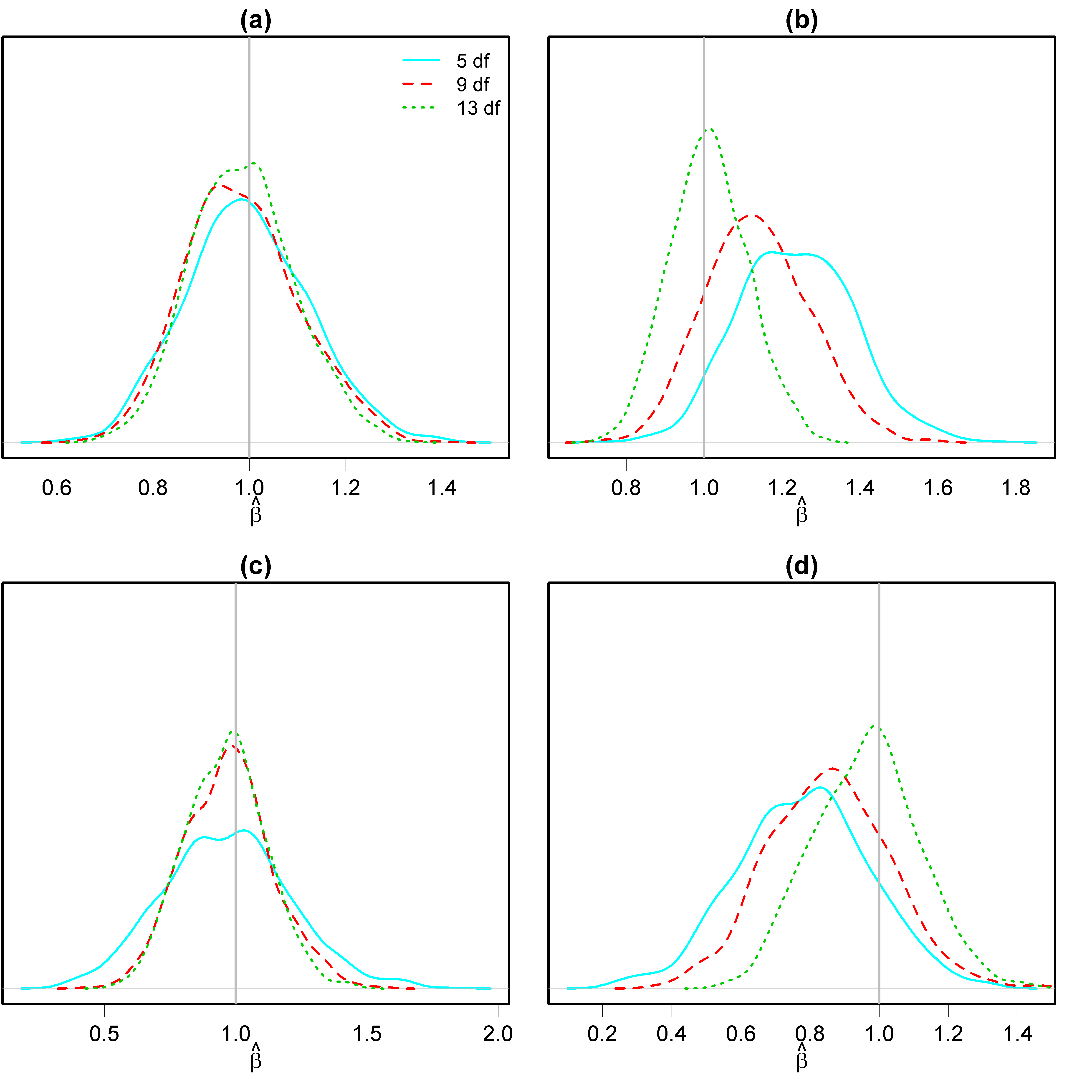
Figure 1: Density plots of $\hat{\beta}$ show bias from $u_{i,BL}$ in the one dimensional simulation scenario with $n^{*}=1000$ when the compatibility conditions are not satisfied (1,000 Monte Carlo simulations for each scenario). (a) Conditions 1 and 2 are satisfied: subject and monitor locations have the same density, and the health model is fit without subject specific covariates. (b) Condition 1 is violated: same as (a) except that $g({\mathbf{s}})$ is uniform on $(0,10)$. (c) Conditions 1 and 2 are satisfied: subject and monitor locations have the same density, the health model is fit with a sinusoidal covariate, and the additional covariate is included in the exposure model. (d) Condition 2 is violated: same as (c) except that the sinusoidal covariate is not included in the exposure model.

To illustrate the bias from the Berkson-like error when either of the compatibility conditions is violated, we set $n^{*}=1000$ so that the classical-like error is negligible. The results of these simulations are shown in Figure 1. In panels (a) and (b), the health model is fit with an intercept but no additional health model covariates, so Condition 2 is automatically satisfied. In panel (a) the density of subject locations $g({\mathbf{s}})$ is the same as $h({\mathbf{s}})$, and there is no evidence of bias in $\hat{\beta}$. In panel (b), $g({\mathbf{s}})$ is uniform on the interval $(0,10)$ so that Condition 1 is violated. There is clear evidence of bias away from the null for $5$ and $9$ df exposure models. There is no evidence of bias with $13$ df, which can be attributed to the fact that the exposure model with $13$ df is sufficiently rich to account for almost all of the spatial structure in $\Phi({\mathbf{s}})$, meaning that the Berkson-like error behaves like pure Berkson error.

In panels (c) and (d) of Figure 1, $g({\mathbf{s}})$ is the same as $h({\mathbf{s}})$, but we fit the health model including an additional covariate $z_{i}=\sin({\mathbf{s}}_{i})$. In panel (c), this covariate is also included in the exposure model, and as expected we see no evidence of bias in $\hat{\beta}$. In panel (d), the additional covariate is not included in the exposure model, so Condition 2 is violated. There is noticeable bias of $\hat{\beta}$ toward the null, especially for the $5$ and $9$ df spline models.

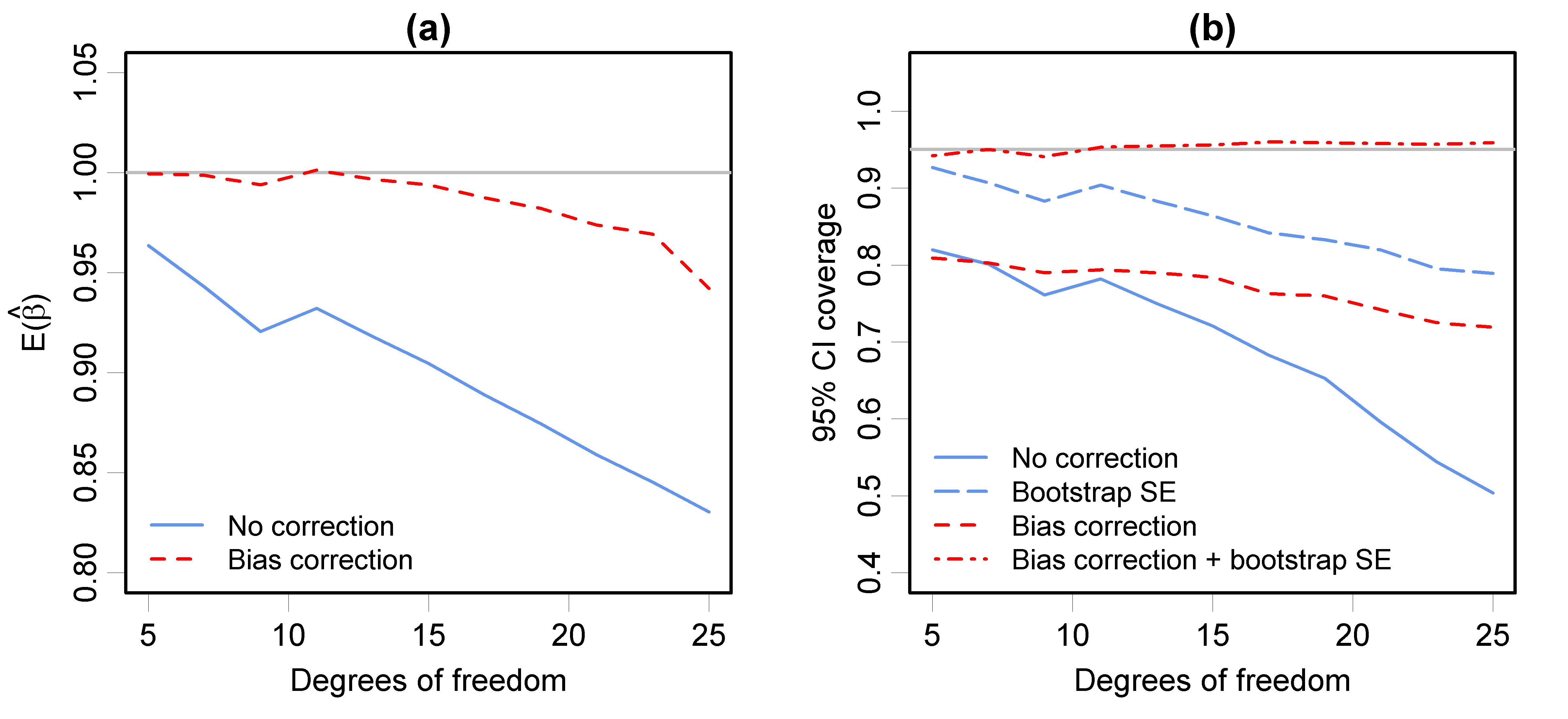
Figure 2: The two-step measurement error correction method adjusts for bias and gives valid standard error estimates in the one dimensional simulation scenario with $n^{*}=200$ (1,000 Monte Carlo simulations for each scenario and 100 bootstrap samples). (a) Uncorrected health effect estimates have noticeable bias, especially for high dimensional exposure models. Our analytical correction successfully adjust for the bias. (b) The combination of bias adjustment and bootstrap standard errors gives 95% confidence intervals with nominal coverage properties. Neither bias adjustment alone nor bootstrap standard errors alone are sufficient.

In Figure 2, we show results from a separate set of simulations with $n^{*}=200$ in order to illustrate the measurement error correction methods from Section 4. In these simulations, $g({\mathbf{s}})$ is the same as $h({\mathbf{s}})$ and the health model is fit without additional covariates, so Conditions 1 and 2 are satisfied. The mean out-of-sample $R^{2}$ ranges from $0.25$ for 5 df to $0.35$ for 13 df, corresponding to the challenging situation of an exposure model with marginal performance that can lead to substantial bias in estimating $\beta$. In panel (a), we see that the uncorrected health effect estimates have notable bias, especially for larger df exposure models, and our correction successfully removes most of the bias. Panel (b) shows the coverage of nominal 95% confidence intervals. In the uncorrected analyses, coverage ranges from 45% to 80%, depending on the df in the exposure model. Confidence intervals that incorporate either the bias correction or bootstrap standard errors improve the coverage. We obtain nearly perfect 95% coverage when we incorporate the bias correction and bootstrap standard errors.

5.2 Spatial exposure surface

Our second set of simulations is based on the MESA Air study design in the Baltimore region (Section 6), using 1,000 simulated datasets and 100 bootstrap samples. We enforce Conditions 1 and 2 and focus on illustrating the value of the correction methods described in Section 4 in a realistic spatial setting. The spatial domain is a $257\times 257$ discrete grid scaled to be a square 30 units on a side. There are $n^{*}=125$ monitor locations, sampled in clusters by first choosing 25 locations i.i.d. uniformly on $S$ and then also including the four nearest neighbors for each such location. Our bootstrap for these simulations resamples clusters of five monitors. A total of $n=600$ subject locations are selected uniformly and independently from $S$.

The predictable part of the exposure surface is

$$\Phi({\mathbf{s}})=\gamma_{0}+\gamma_{1}R_{1}({\mathbf{s}})+\gamma_{2}R_{2}({\mathbf{s}})+\gamma_{3}R_{3}({\mathbf{s}})+\Phi_{1}({\mathbf{s}}).$$

Each $\gamma_{i}=4.9$, and each $R_{k}({\mathbf{s}})$ is constructed by drawing i.i.d. realizations from $N(0,1/3)$ at each ${\mathbf{s}}\in S$. $\Phi_{1}({\mathbf{s}})$ is a fixed realization from a spectral approximation to a Gaussian field with Matérn covariance (Paciorek 2007) with range 20 and unit differentiability parameter, normalized such that the variance of $\Phi_{1}({\mathbf{s}})$ on $S$ is 30. Thus the total variance of $\Phi({\mathbf{s}})$ on $S$ is approximately 54. In the true exposure surface and monitoring data, there is also a nugget with variance $\sigma^{2}_{\eta}=\sigma^{2}_{\eta^{*}}=6$. We consider two spatial scenarios, corresponding to different fixed realizations of $\Phi_{1}({\mathbf{s}})$. These surfaces are shown in Figure 3.

The spatial exposure model has ${\mathbf{R}}({\mathbf{s}})$ comprised of $R_{k}({\mathbf{s}})$ for $k=1,2,3$ and a thin-plate spline basis derived by fitting a GAM from the MGCV package in R (Wood 2006) to the observed monitoring data with fixed degrees of freedom (df). Thus the spatial basis is actually different for each simulated dataset since it depends on the monitor locations, but we keep the same basis functions for the bootstrap analysis within each simulation run. We estimate the standard error of $\hat{{\boldsymbol{\gamma}}}$ using a sandwich estimator for clustered data implemented in the R package geepack (Hojsgaard et al. 2006).

The true and fitted health models have an intercept but no additional covariates. We set $\beta=0.1$ and consider i.i.d. normally distributed $\epsilon\sim N(0,\sigma^{2}_{\epsilon})$ with $\sigma^{2}_{\epsilon}$ equal to 200 or 10. The larger value of $\sigma^{2}_{\epsilon}=200$ is consistent with what we see in the MESA Air data with left ventricular mass index (LVMI) as the outcome, where the air pollution exposure explains approximately $0.3\%$ of the variance after adjustment for known risk factors. We also consider $\sigma^{2}_{\epsilon}=10$ such that air pollution exposure explains approximately $5\%$ of the health outcome variance in order to see more clearly the potential impact of exposure measurement error.

The two spatial surfaces, while generated at random, represent different deterministic scenarios in which we could find ourselves (e.g., different metropolitan areas). In scenario 1 the spatially structured part of the air pollution surface $\Phi_{1}({\mathbf{s}})$ can be represented fairly well using thin-plate splines with either 5 or 10 df, while the spatial surface in scenario 2 cannot be represented well with 5 df but can be reasonably well modeled with 10 df. This is reflected in the $R^{2}$ values in Figure 3, which represent the best thin-plate spline fits to the surfaces, assuming essentially unlimited monitoring data is available. The cross-validated and out-of-sample $R^{2}$ values for predicting the full air pollution surface $\Phi({\mathbf{s}})$ (including non-spatially structured covariates) based on monitoring data reported in Table 1 exhibit a similar pattern. For leave-one-out cross-validation, the clusters of five adjacent monitors are treated as a single unit.

We focus our discussion on the scenarios with $\sigma^{2}_{\epsilon}=10$ because this is where the impact of exposure measurement error is most prominent. The measurement error impact is qualitatively similar for $\sigma^{2}_{\epsilon}=200$, but it is less important because the unmodeled variability in the health outcome dominates. Our theory dictates that the relative biases for $\sigma^{2}_{\epsilon}=10$ and $\sigma^{2}_{\epsilon}=200$ are identical, which we verified in simulations out to four significant digits, so we only report one value.

When we fit the exposure model with a 5 df thin-plate spline, there is modest bias toward the null of $3\%$ in scenario 1 and more substantial bias of $12\%$ in scenario 2. Our asymptotic correction reduces the magnitude of bias in both instances. The bias correction followed by bootstrap standard errors consistently gives valid inference, including accurate standard error estimates and nominal coverage of $95\%$ confidence intervals. In scenario 1, we also get valid inference with bootstrap standard errors and no bias correction.

When we increase the complexity of the spatial model to 10 df, prediction accuracy improves in both scenarios, but inference about the health effect parameter is degraded. The magnitude of bias is approximately the same as with 5 df, but our asymptotic correction is less effective. Furthermore, the bootstrap standard error estimates tend to be too large, resulting in over-coverage of 95% confidence intervals. These findings are not surprising, because while each simulated dataset has $125$ monitor locations, they are clustered in groups of $5$ so that there are effectively only $25$ unique locations for estimating the smooth component of the spatial surface, so a thin-plate spline model with 10 df overfits these data in the sense that we do not expect to be able to rely on large $n^{*}$ asymptotic approximations such as (LABEL:eq:cl.bias) or the nonparametric bootstrap.

6 Data analysis

The Multi-Ethnic Study of Atherosclerosis and Air Pollution (MESA Air) is an ongoing cohort study designed to investigate the relationship between air pollution exposure and progression of subclinical atherosclerosis (Bild et al. 2002; Kaufman et al. 2012). The MESA Air cohort includes over 6,000 subjects in six U.S. metropolitan areas (Baltimore City and Baltimore County, MD; Chicago, IL; Forsyth County (Winston-Salem), NC; Los Angeles and Riverside Counties, CA; New York and Rockland County, NY; and St Paul, MN). Four ethnic/racial groups were targeted, white, African American, Hispanic, and Chinese American, and all study participants (46 to 87 years of age) were without clinical cardiovascular disease at the baseline examination (2000–-2002). An early cross-sectional finding from MESA Air is that an elevated left-ventricular mass index (LVMI) is associated with exposure to traffic related air pollution, specifically outdoor residential concentrations of gaseous oxides of nitrogen (NOx) (Van Hee et al. 2009, 2012). Van Hee et al. (2012) found that an increase in NOx concentration of 10 parts per billion (ppb) is associated with a 0.36 $g/m^{2}$ increase in LVMI (95% CI: 0.02 - 0.7 $g/m^{2}$).

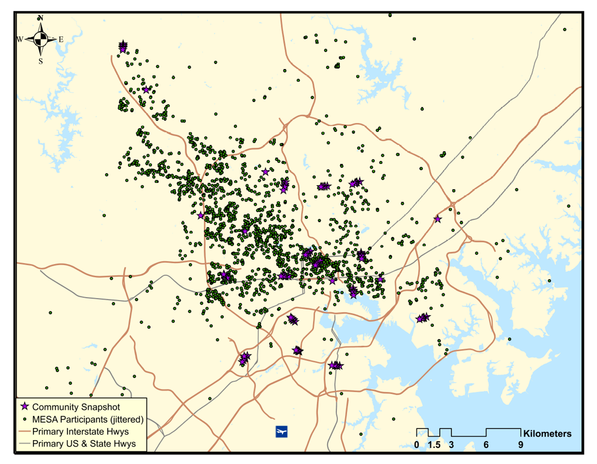
Figure 4: Subject and monitor locations in the Baltimore MESA Air dataset.

Van Hee et al. (2012) utilized predictions from a spatio-temporal exposure model that incorporates regulatory and study-specific monitoring data in all six regions (Szpiro et al. 2010b). To illustrate our methodology for a purely spatial exposure model, we re-analyze the data restricted to subjects in the Baltimore region, and we construct an exposure model based on data from three community snapshot monitoring campaigns conducted by MESA Air. In brief, the community snapshot campaign consisted of three separate rounds of spatially rich sampling during single two-week periods in different seasons. In the Baltimore area, approximately 100 measurements were made in each of three two-week periods in May 2006, November 2006, and February 2007. In each round of snapshot monitoring, the majority of monitors were arranged in clusters of six, with three on either side of a major road at distances of approximately 50, 100, and 300 meters (Cohen et al. 2009). In addition, the locations were chosen to characterize different land use categories and to cover the geographic region as broadly as possible. To help with satisfying Condition 1, we exclude one cluster from our analysis because it is far from any of the study subjects, and we approximate long-term average concentrations by averaging the three available measurements at locations that were monitored in all three seasons. The 93 monitor locations and 625 subject locations in our analysis are shown in Figure 4.

Our exposure model incorporates five geographic covariates: (i) distance to a major road, (ii) local-source traffic pollution from a dispersion model (Wilton et al. 2010), (iii) population density in a 1 km buffer, (iv) distance to downtown, and (v) transportation land use in a 1 km buffer. The first three of these geographic covariates are log-transformed. An additional covariate describing the density of high-intensity land-use (commercial, industrial, residential, etc.) was also incorporated in the original spatio-temporal model predictions used by (Van Hee et al. 2012), but we exclude this covariate from our model because it has very different distributions across subject and monitor locations, a clear violation of Condition 1. To account for unmodeled spatial structure, we use a thin-plate spline basis with 0, 5, or 10 df, constructed as in the simulations. We estimate the standard error of $\hat{{\boldsymbol{\gamma}}}$ using a sandwich estimator for clustered data implemented in the R package geepack (Hojsgaard et al. 2006). We estimate the association between NOx and LVMI by fitting a multivariate linear regression, including an exhaustive set of additional health model covariates that could be potential confounders (Van Hee et al. 2009).

The results of our analysis are shown in Table 2, with 10,000 bootstrap replicates (resampling clusters of monitors, where applicable). Our findings are very similar for an exposure model that is purely land-use regression and one that includes splines with 5 df. We estimate that an increase in NOx concentration of 10 parts per billion (ppb) is associated with approximately a 0.7 $g/m^{2}$ increase in LVMI. Our standard error estimates for these models in Table 2 range from $0.55$ to $0.68$ $g/m^{2}$, so the difference in effect size from that found by Van Hee et al. (2012) is very likely due to our more limited dataset. The exposure model that includes 5 df splines has a larger cross-validated $R^{2}$, suggesting that it captures more variability in the exposure. This translates into a smaller model-based standard error, but this apparent advantage is attenuated when we correct for exposure measurement error with bootstrap standard error estimates, and it goes away entirely when we also incorporate the bias correction.

The exposure model with 10 df gives slightly larger effect estimates and standard errors. There is also more evidence of bias from classical-like error than for the lower dimensional exposure models. However, our simulation results in Table 1 suggest that a 10 df spline is too rich of a model for the available monitoring data and that these results should be considered less reliable than those based on 5 df splines.

7 Discussion

We have developed a statistical framework for characterizing and correcting measurement error in two-stage analyses, focusing particularly on problems where a first-stage spatial model is used to predict exposure that is measured at different locations than are needed in a second-stage health analysis. Our methodology is robust to misspecification of the exposure model, treating it as a device to explain some portion of the variability in exposure. We adopt a design-based perspective in which the process of selecting exposure measurement and subject locations is the primary source of spatial randomness, leading naturally to nonparametric bootstrap resampling for standard errors. A major contribution of our work is that we delineate the potential sources of bias from Berkson-like and classical-like measurement error and provide strategies for reducing bias and variance at the design and analysis stages. Bias from classical-like error can be corrected using an asymptotic approximation, whereas bias from Berkson-like error should be addressed at the design stage or when selecting an exposure model.

While our research is primarily motivated by epidemiologic analysis of long-term air pollution health effects, we note that the spatial prediction problem can be interpreted as a linear model. Thus, our measurement error decomposition, asymptotic results, and bias correction hold equally well in non-spatial settings.

Our theory and simulations demonstrate that bias from the classical-like error is small when the exposure model is not overfit in the sense that there are sufficient observations relative to the dimension of the exposure model for the large $n^{*}$ asymptotics to be relevant. The limited magnitude of the bias suggests that measurement error correction efforts should focus on avoiding overfitting the exposure model and satisfying the conditions needed to ensure that Berkson-like error does not induce important bias (at least in a linear health model). Nonetheless, in several simulation scenarios our asymptotic correction for bias from classical-like error results in improved estimation and inference, even at the expense of increased variance. Indeed, in our analyses and simulations the increased variance caused by estimating the bias is modest.

Our theoretical development motivates the use of a nonparametric bootstrap to account for variability induced by measurement error. When the bias correction is not used, simulations suggest that the underestimation of uncertainty from ignoring the measurement error (using a sandwich variance estimator) is modest, but even so there are cases in which accounting for the effect of measurement error is necessary. When we include the asymptotic bias correction, the bootstrap is more generally necessary for valid confidence intervals.

As we remarked in Section 2.3, exposure model selection is a broad topic and a specific algorithm for selecting geographic covariates or spline basis functions is beyond the scope of this paper. However, we discuss below several practical approaches that can be considered in designing a study to approximately satisfy the compatibility conditions from Section 2.3, so as to minimize the bias from Berkson-like error. We will explore these options and related tradeoffs further in future work.

First, to satisfy Condition 1, as much care as possible should be taken at the design stage to ensure the sampling densities of locations and exposure covariates are as similar as possible in the first-stage exposure observations and the second-stage outcome observations. While this criterion is overly abstract in the context of a specific study, the practical implication is that first-stage and second-stage locations should be chosen to be similar in terms of location and pertinent covariates. If exposure data have already been collected, it may be necessary to consider excluding exposure or outcome data or deleting one or more covariates from ${\mathbf{R}}({\mathbf{s}})$ in order to minimize the mismatch.

If we are particularly concerned about Condition 2, we can add terms to ${\mathbf{R}}({\mathbf{s}})$ to span ${\mathbf{\Theta}}({\mathbf{s}})$. We generally will not know ${\mathbf{\Theta}}({\mathbf{s}})$ directly, but if we do (e.g., if household income were known and monitors were located at homes) then supplementing ${\mathbf{R}}({\mathbf{s}})$ with ${\mathbf{\Theta}}({\mathbf{s}})$ or projecting ${\mathbf{R}}({\mathbf{s}})$ to make it orthogonal to ${\mathbf{\Theta}}({\mathbf{s}})$ are equivalent. In most realistic settings, we will assume that ${\mathbf{\Theta}}({\mathbf{s}})$ is a set of smooth functions of space that can be modeled by spline terms, but we will not know the minimal spanning spline basis. In this case it is preferable to supplement ${\mathbf{R}}({\mathbf{s}})$ with as rich of a basis as possible without introducing substantial classical-like error. Projecting ${\mathbf{R}}({\mathbf{s}})$ to make it orthogonal to a similarly rich spline basis would likely result in a significant diminution of exposure variability beyond what is needed to eliminate bias from not satisfying Condition 2.

The possibility of adding dimensions to ${\mathbf{R}}({\mathbf{s}})$ highlights the critical tradeoff between Berkson-like and classical-like error. Augmenting ${\mathbf{R}}({\mathbf{s}})$ reduces Berkson-like error by accounting for more of the variability in $w({\mathbf{s}})$. Since eliminating Berkson-like error also eliminates the need to satisfy the compatibility conditions, we generally expect that adding such terms will limit bias from the Berkson-like error. A side effect of augmenting ${\mathbf{R}}({\mathbf{s}})$ is to change the sampling variability of $\hat{{\boldsymbol{\gamma}}}$, which impacts the classical-like error. This could be beneficial if the additional terms in ${\mathbf{R}}({\mathbf{s}})$ account for a substantial amount of variability in $w({\mathbf{s}})$, since the result will be to reduce the variance of the original components of $\hat{{\boldsymbol{\gamma}}}$. On the other hand, if the coefficients for the new terms are difficult to estimate, the result will be a substantial new contribution to the classical-like error, leading to additional bias and variance in the second-stage estimation. In fact, in order to reduce classical-like error, one might choose to remove selected dimensions from ${\mathbf{R}}({\mathbf{s}})$ if their coefficients are particularly difficult to estimate.

There are some key assumptions in our model that may not be strictly satisfied in air pollution epidemiology studies. First, we regard the sets of locations of exposure and health observations to be independent, or at least independent clusters. This assumption can be questioned, particularly in the case of air pollution monitors, as one would not expect a government agency to select two sites that are very close together. Second, a major source of exposure heterogeneity that we do not consider is the difference between exposure at a residence and the exposure experienced by individuals when they are not home. Mobility may be less important in studies of small children and the elderly, but this remains an open issue in the epidemiologic literature.

Finally, as described in Section 2.1, we condition on the unobserved but deterministic spatial variation in exposure during the time period of the study. This avoids having to postulate that one could meaningfully repeat the experiment in other time periods. This is particularly important when the averaging period of interest is one or more years since secular trends in the nature and sources of air pollution limit the number of years during which air pollution studies can be regarded as answering analogous scientific questions. For shorter-term studies, there is additional variability associated with the choice of time period, and it would be reasonable to regard the different air pollution surfaces at different times as arising from a random spatial process. However, with data from only a single time period and a misspecified mean model, it is impossible to identify both the fixed and random components of the spatial residuals, so we do not incorporate a random effect in our formulation.

Our measurement error correction is based on asymptotic approximations derived for linear regression for the exposure and health models. Real world applications often involve additional complications, suggesting further research directions. On the exposure model side, our methods can be extended to penalized models and full-rank models such as universal kriging and related spatio-temporal models that are often used in environmental studies. Nonlinear models such as logistic regression and Cox regression are commonly used for the second stage in health studies, and it is also important to consider the implications of misspecification in the second-stage model, in addition to the exposure model.

Two-stage analyses to date have taken the approach of optimizing the exposure model for exposure prediction accuracy, based on the implicit assumption that this will also lead to optimal second-stage health effect inference. In previous work we have shown that optimizing the exposure model for prediction accuracy can be sub-optimal for health effects estimation (Szpiro et al. 2011a). An interesting avenue for future research involves developing methods to optimize the exposure model for estimation of the health effect of interest in the second-stage model. A final direction for additional research that is of great interest in air pollution epidemiology is to extend these methods for measurement error correction when assessing health effects of multiple exposures or mixtures of exposures. When predictions for more than one exposure are used in a health model, there is the possibility of a form of omitted variable bias from components of variability that are missing from the predictions of the exposures.

Appendix A Proof of of Lemma 2

Proof of Lemma 2.

By definition, $\hat{\beta}_{\infty,n^{*}}$ is the ’true’ parameter value in a linear model for $y$ on $\hat{w}({\mathbf{s}})$ and covariates, ${\mathbf{z}}$, so we can express

$$y_{i}=\hat{\beta}_{\infty,n^{*}}\hat{w}({\mathbf{s}}_{i})+\hat{{\boldsymbol{\beta}}}_{z,\infty,n^{*}}^{\top}{\mathbf{z}}_{i}+\nu_{i},$$

for some $\hat{{\boldsymbol{\beta}}}_{z,\infty,n^{*}}$ and an error term, $\nu_{i}$, that is orthogonal to $\hat{w}({\mathbf{s}}_{i})$ and to the elements of ${\mathbf{z}}_{i}$ with respect to the density $g({\mathbf{s}})$. We can rewrite this expression as

$$y_{i}=\hat{\beta}_{\infty,n^{*}}\hat{w}^{c}({\mathbf{s}}_{i})+\left(\hat{{\boldsymbol{\beta}}}_{z,\infty,n^{*}}^{\top}{\mathbf{z}}_{i}+\nu_{i}+\hat{\beta}_{\infty,n^{*}}(\hat{w}({\mathbf{s}}_{i})-\hat{w}^{c}({\mathbf{s}}_{i}))\right)$$ (A.1)

and note that each of the last three terms is orthogonal to $\hat{w}^{c}({\mathbf{s}}_{i})$. Given this orthogonality, we can view the last three terms as a single error term. The OLS solution for this no-intercept linear model,

$$\frac{\sum_{i=1}^{n}y_{i}\hat{w}^{c}({\mathbf{s}}_{i})}{\sum_{i=1}^{n}\hat{w}^{c}({\mathbf{s}}_{i})^{2}},$$ (A.2)

converges a.s. to $\hat{\beta}_{\infty,n^{*}}$ for any fixed $n^{*}$ based on Lemma 1 of White (1980). We can express each observation as

$$y_{i}=\beta w^{c}({\mathbf{s}}_{i})+\beta(w({\mathbf{s}}_{i})-w^{c}({\mathbf{s}}_{i}))+\beta({\mathbf{\Phi}}({\mathbf{s}}_{i})-w({\mathbf{s}}_{i}))+\beta\eta_{i}+{\boldsymbol{\beta}}_{z}^{\top}{\mathbf{z}}_{i}+\epsilon_{i}$$ (A.3)

and plug in for $y_{i}$ in (A.2). Taking the limit as $n\to\infty$ shows that the a.s. limit of (A.2) can be expressed as

$$\hat{\beta}_{\infty,n^{*}}=\beta\frac{\int w^{c}({\mathbf{s}})\hat{w}^{c}({\mathbf{s}})dG({\mathbf{s}})}{\int\hat{w}^{c}({\mathbf{s}})^{2}dG({\mathbf{s}})},$$ (A.4)

where the limiting value on the right hand side is found by dividing the numerator and denominator of (A.2) by $n$ and invoking the law of large numbers. In the numerator, only the first summand in the expression for $y_{i}$ gives a non-zero contribution. The contribution from the second summand is zero because $(w({\mathbf{s}}_{i})-w^{c}({\mathbf{s}}_{i}))$ is a linear combination of elements of ${\mathbf{\Theta}}({\mathbf{s}})$ while $w^{c}({\mathbf{s}})$ is orthogonal to each component of ${\mathbf{\Theta}}({\mathbf{s}})$. For the third summand, we use our assumption that Condition 2 is satisfied. Namely, $w^{c}({\mathbf{s}})$ is a linear combination of elements of ${\mathbf{\Theta}}({\mathbf{s}})$ and ${\mathbf{R}}({\mathbf{s}})$, so it is sufficient for $({\mathbf{\Phi}}({\mathbf{s}}_{i})-w({\mathbf{s}}_{i}))$ to be orthogonal to each of the elements of ${\mathbf{\Theta}}({\mathbf{s}})$ and ${\mathbf{R}}({\mathbf{s}})$, and this is guaranteed if the elements of ${\mathbf{\Theta}}({\mathbf{s}})$ are in the span of ${\mathbf{R}}({\mathbf{s}})$ as required by Condition 2.

We now define the $p\times p$ matrix ${\mathbf{A}}=\int{\mathbf{R}}^{c}({\mathbf{s}})^{\top}{\mathbf{R}}^{c}({\mathbf{s}})dG({\mathbf{s}})$ and set

$$f(\hat{{\boldsymbol{\gamma}}})=\left({\boldsymbol{\gamma}}^{\top}{\mathbf{A}}\hat{{\boldsymbol{\gamma}}}\right)\left(\hat{{\boldsymbol{\gamma}}}^{\top}{\mathbf{A}}\hat{{\boldsymbol{\gamma}}}\right)^{-1},$$

so that $\hat{\beta}_{\infty,n^{*}}=\beta f({\boldsymbol{\gamma}})$. The gradient of $f(\hat{{\boldsymbol{\gamma}}})$ is

$$Df(\hat{{\boldsymbol{\gamma}}})=-2({\boldsymbol{\gamma}}^{\top}{\mathbf{A}}\hat{{\boldsymbol{\gamma}}})(\hat{{\boldsymbol{\gamma}}}^{\top}{\mathbf{A}}\hat{{\boldsymbol{\gamma}}})^{-2}{\mathbf{A}}\hat{{\boldsymbol{\gamma}}}+(\hat{{\boldsymbol{\gamma}}}^{\top}{\mathbf{A}}\hat{{\boldsymbol{\gamma}}})^{-1}{\mathbf{A}}{\boldsymbol{\gamma}},$$

and its Hessian is

$$D^{2}f(\hat{{\boldsymbol{\gamma}}}) = {}-2({\boldsymbol{\gamma}}^{\top}{\mathbf{A}}\hat{{\boldsymbol{\gamma}}})(\hat{{\boldsymbol{\gamma}}}^{\top}{\mathbf{A}}\hat{{\boldsymbol{\gamma}}})^{-2}{\mathbf{A}}+8({\boldsymbol{\gamma}}^{\top}{\mathbf{A}}\hat{{\boldsymbol{\gamma}}})(\hat{{\boldsymbol{\gamma}}}^{\top}{\mathbf{A}}\hat{{\boldsymbol{\gamma}}})^{-3}{\mathbf{A}}\hat{{\boldsymbol{\gamma}}}\hat{{\boldsymbol{\gamma}}}^{\top}{\mathbf{A}}$$

$${}-2(\hat{{\boldsymbol{\gamma}}}^{\top}{\mathbf{A}}\hat{{\boldsymbol{\gamma}}})^{-2}{\mathbf{A}}\hat{{\boldsymbol{\gamma}}}{{\boldsymbol{\gamma}}}^{\top}{\mathbf{A}}-2(\hat{{\boldsymbol{\gamma}}}^{\top}{\mathbf{A}}\hat{{\boldsymbol{\gamma}}})^{-2}{\mathbf{A}}{{\boldsymbol{\gamma}}}\hat{{\boldsymbol{\gamma}}}^{\top}{\mathbf{A}}.$$

A second order Taylor expansion of $f(\hat{{\boldsymbol{\gamma}}})$ can be written

$$f(\hat{{\boldsymbol{\gamma}}}) \approx 1-({\boldsymbol{\gamma}}^{\top}{\mathbf{A}}{\boldsymbol{\gamma}})^{-1}(\hat{{\boldsymbol{\gamma}}}-{\boldsymbol{\gamma}})^{\top}{\mathbf{A}}{\boldsymbol{\gamma}}-({\boldsymbol{\gamma}}^{\top}{\mathbf{A}}{\boldsymbol{\gamma}})^{-1}(\hat{{\boldsymbol{\gamma}}}-{\boldsymbol{\gamma}})^{\top}{\mathbf{A}}(\hat{{\boldsymbol{\gamma}}}-{\boldsymbol{\gamma}})$$

$${}+2({\boldsymbol{\gamma}}^{\top}{\mathbf{A}}{\boldsymbol{\gamma}})^{-2}(\hat{{\boldsymbol{\gamma}}}-{\boldsymbol{\gamma}})^{\top}{\mathbf{A}}{\boldsymbol{\gamma}}{\boldsymbol{\gamma}}^{\top}{\mathbf{A}}(\hat{{\boldsymbol{\gamma}}}-{\boldsymbol{\gamma}})$$

$$= 1-\frac{\int\left(\hat{w}^{c}({\mathbf{s}})-w^{c}({\mathbf{s}})\right)w^{c}({\mathbf{s}})dG({\mathbf{s}})}{\int w^{c}({\mathbf{s}})^{2}dG({\mathbf{s}})}-\frac{\int\left(\hat{w}^{c}({\mathbf{s}})-w^{c}({\mathbf{s}})\right)^{2}dG({\mathbf{s}})}{\int w^{c}({\mathbf{s}})^{2}dG({\mathbf{s}})}$$

$${}+2\frac{\left(\int\left(\hat{w}^{c}({\mathbf{s}})-w^{c}({\mathbf{s}})\right)w^{c}({\mathbf{s}})dG({\mathbf{s}})\right)^{2}}{\left(\int w^{c}({\mathbf{s}})^{2}dG({\mathbf{s}})\right)^{2}}$$

$$= 1-\frac{\int\left(\hat{w}^{c}({\mathbf{s}})-w^{c}({\mathbf{s}})\right)w^{c}({\mathbf{s}})dG({\mathbf{s}})}{\int w^{c}({\mathbf{s}})^{2}dG({\mathbf{s}})}-\frac{\int\left(\hat{w}^{c}({\mathbf{s}})-w^{c}({\mathbf{s}})\right)^{2}dG({\mathbf{s}})}{\int w^{c}({\mathbf{s}})^{2}dG({\mathbf{s}})}$$

$${}+2\frac{\int\left(\hat{w}^{c}({\mathbf{s}}_{1})-w^{c}({\mathbf{s}}_{1})\right)\left(\hat{w}^{c}({\mathbf{s}}_{2})-w^{c}({\mathbf{s}}_{2})\right)w^{c}({\mathbf{s}}_{1})w^{c}({\mathbf{s}}_{2})dG({\mathbf{s}}_{1})dG({\mathbf{s}}_{2})}{\left(\int w^{c}({\mathbf{s}})dG({\mathbf{s}})\right)^{2}}$$

We require sufficient regularity such that the higher order terms converge in distribution to zero sufficiently fast as $n^{*}\rightarrow\infty$. Equations (LABEL:eq:cl.bias) and (3.7) are then derived by taking the asymptotic expectation and asymptotic variance of the expression above (for the asymptotic variance, we can restrict our attention to the first non-constant term above). This requires interchanging asymptotic expectations with respect to $\hat{{\boldsymbol{\gamma}}}$ with integrals in ${\mathbf{s}}$. A sufficient condition to do this is that ${\mathbf{R}}({\mathbf{s}})$ is bounded as a function of ${\mathbf{s}}$. The interchange is accomplished by expressing asymptotic expectations as standard expectations of the appropriate limiting distributions of functions of $\sqrt{n^{*}}(\hat{{\boldsymbol{\gamma}}}-{\boldsymbol{\gamma}})$ using Definition 1, invoking the continuous mapping theorem to express these limiting distributions as functions of the limiting distribution of $\sqrt{n^{*}}(\hat{{\boldsymbol{\gamma}}}-{\boldsymbol{\gamma}})$, and then using the Fubini-Tonelli theorem (Folland 1999) to exchange the order of integration between $\hat{{\boldsymbol{\gamma}}}$ and of ${\mathbf{s}}$. There is an additional step to express asymptotic expectations as the asymptotic covariances in (LABEL:eq:cl.bias) and (3.7). We use Definition 1 to express the asymptotic expectations as standard expectations of the appropriate limiting distributions of functions of $\sqrt{n^{*}}(\hat{{\boldsymbol{\gamma}}}-{\boldsymbol{\gamma}})$, again invoke the continuous mapping theorem, express the resulting expectations as covariances of the limiting distributions of functions of $\sqrt{n^{*}}(\hat{{\boldsymbol{\gamma}}}-{\boldsymbol{\gamma}})$, and finally write the resulting expression as asymptotic covariances using Definition 1. ∎

Appendix B Estimating the asymptotic bias

To estimate the asymptotic bias based on (3.8), we require the second derivatives, $\frac{\partial^{2}\kappa}{\partial m_{j}\partial m_{k}}$. Differentiating with respect to $m_{j}$ and $m_{k}$ gives us a long expression involving first and second derivatives of $M$:

$$\big{(}{\mathbf{R}}^{*^{\top}}{\mathbf{M}}{\mathbf{R}}^{*}\big{)}^{-1}{\mathbf{R}}^{*^{\top}}\frac{\partial{\mathbf{M}}}{\partial m_{k}}{\mathbf{R}}^{*}\big{(}{\mathbf{R}}^{*^{\top}}{\mathbf{M}}{\mathbf{R}}^{*}\big{)}^{-1}{\mathbf{R}}^{*^{\top}}\frac{\partial{\mathbf{M}}}{\partial m_{j}}{\mathbf{R}}^{*}\big{(}{\mathbf{R}}^{*^{\top}}{\mathbf{M}}{\mathbf{R}}^{*}\big{)}^{-1}{\mathbf{R}}^{*^{\top}}{\mathbf{M}}{\mathbf{\Phi}}^{*}-$$

$$\big{(}{\mathbf{R}}^{*^{\top}}{\mathbf{M}}{\mathbf{R}}^{*}\big{)}^{-1}{\mathbf{R}}^{*^{\top}}\frac{\partial^{2}{\mathbf{M}}}{\partial m_{j}\partial m_{k}}{\mathbf{R}}^{*}\big{(}{\mathbf{R}}^{*^{\top}}{\mathbf{M}}{\mathbf{R}}^{*}\big{)}^{-1}{\mathbf{R}}^{*^{\top}}{\mathbf{M}}{\mathbf{\Phi}}^{*}+$$

$$\big{(}{\mathbf{R}}^{*^{\top}}{\mathbf{M}}{\mathbf{R}}^{*}\big{)}^{-1}{\mathbf{R}}^{*^{\top}}\frac{\partial{\mathbf{M}}}{\partial m_{j}}{\mathbf{R}}^{*}\big{(}{\mathbf{R}}^{*^{\top}}{\mathbf{M}}{\mathbf{R}}^{*}\big{)}^{-1}{\mathbf{R}}^{*^{\top}}\frac{\partial{\mathbf{M}}}{\partial m_{k}}{\mathbf{R}}^{*}\big{(}{\mathbf{R}}^{*^{\top}}{\mathbf{M}}{\mathbf{R}}^{*}\big{)}^{-1}{\mathbf{R}}^{*^{\top}}{\mathbf{M}}{\mathbf{\Phi}}^{*}-$$

$$\big{(}{\mathbf{R}}^{*^{\top}}{\mathbf{M}}{\mathbf{R}}^{*}\big{)}^{-1}{\mathbf{R}}^{*^{\top}}\frac{\partial{\mathbf{M}}}{\partial m_{j}}{\mathbf{R}}^{*}\big{(}{\mathbf{R}}^{*^{\top}}{\mathbf{M}}{\mathbf{R}}^{*}\big{)}^{-1}{\mathbf{R}}^{*^{\top}}\frac{\partial{\mathbf{M}}}{\partial m_{k}}{\mathbf{\Phi}}^{*}-$$

$$\big{(}{\mathbf{R}}^{*^{\top}}{\mathbf{M}}{\mathbf{R}}^{*}\big{)}^{-1}{\mathbf{R}}^{*^{\top}}\frac{\partial{\mathbf{M}}}{\partial m_{k}}{\mathbf{R}}^{*}\big{(}{\mathbf{R}}^{*^{\top}}{\mathbf{M}}{\mathbf{R}}^{*}\big{)}^{-1}{\mathbf{R}}^{*^{\top}}\frac{\partial{\mathbf{M}}}{\partial m_{j}}{\mathbf{\Phi}}^{*}+$$

$$\big{(}{\mathbf{R}}^{*^{\top}}{\mathbf{M}}{\mathbf{R}}^{*}\big{)}^{-1}{\mathbf{R}}^{*^{\top}}\frac{\partial^{2}{\mathbf{M}}}{\partial m_{j}\partial m_{k}}{\mathbf{\Phi}}^{*}.$$

The first derivative with respect to $m_{j}$ is a matrix of zeros with a single one in the $j$th diagonal position, while the second partial derivative is a matrix of zeros. The terms that remain in the expression can be easily calculated based on the observed ${\mathbf{R}}^{*}$ and using the plug-in estimate, ${\mathbf{X}}^{*}=(x_{1}^{*},\ldots,x_{n^{*}}^{*})^{\top}$, for ${\mathbf{\Phi}}^{*}$. Note that ${\mathbf{R}}^{*\top}\frac{\partial{\mathbf{M}}}{\partial m_{j}}{\mathbf{R}}^{*}={\mathbf{R}}_{j}^{*}{\mathbf{R}}_{j}^{*\top}$, where ${\mathbf{R}}_{j}^{*}$ is the $j$th row of ${\mathbf{R}}^{*}$, and ${\mathbf{R}}^{*\top}\frac{\partial{\mathbf{M}}}{\partial m_{j}}{\mathbf{X}}^{*}={\mathbf{R}}_{j}^{*\top}x_{j}^{*}$.

$$\begin{array}[]{ccc}\textrm{Scenario 1}&\textrm{5 df }(R^{2}=0.78)&\textrm{10 df }(R^{2}=0.91)\\ \includegraphics[width=144.54pt]{spatial_sim_df_5_vareps_200_seed_100_exact.png}&\includegraphics[width=144.54pt]{spatial_sim_df_5_vareps_200_seed_100_df5.png}&\includegraphics[width=144.54pt]{spatial_sim_df_10_vareps_200_seed_100_df10.png}\\ \textrm{Scenario 2}&\textrm{5 df }(R^{2}=0.22)&\textrm{10 df }(R^{2}=0.63)\\ \includegraphics[width=144.54pt]{spatial_sim_df_5_vareps_200_seed_200_exact.png}&\includegraphics[width=144.54pt]{spatial_sim_df_5_vareps_200_seed_200_df5.png}&\includegraphics[width=144.54pt]{spatial_sim_df_10_vareps_200_seed_200_df10.png}\\ \end{array}$$

Figure 3: Spatial component of the exposure surface for each of two scenarios in the spatial simulation study based on MESA Air. Each scenario corresponds to a different random draw of $\Phi_{1}(\cdot)$ from a Matérn-based Gaussian process with range 20, differentiability parameter 1, and variance on $S\subset\mathbb{R}^{2}$ of 30. The first column is the true surface, and the second and third columns show prediction surfaces and $R^{2}$ from approximating $\Phi_{1}({\mathbf{s}})$ with thin-plate splines using the indicated degrees of freedom, based on fitting a fixed degree-of-freedom spatial GAM model to $\Phi_{1}({\mathbf{s}})$ with observations at every location on the $257\times 257$ grid $S$.

Table 1: Results for spatial simulation (1,000 Monte Carlo simulations for each scenario and 100 bootstrap samples). The average out-of-sample $R^{2}$ is given in parentheses for each exposure model. The first column is the relative bias in estimating $\beta=0.1$. This is the same for $\sigma^{2}=200$ and $\sigma^{2}=10$ and is estimated from 100,000 Monte Carlo samples, resulting in negligible Monte Carlo error. The final six columns show the standard deviation, average estimated standard error, and 95$\%$ confidence interval coverage, separately for $\sigma_{\epsilon}^{2}=200$ and $\sigma_{\epsilon}^{2}=10$.

$$\begin{array}[]{lrrrrrrr}\vspace{0.05cm}\cr&&\lx@intercol\hfil\sigma^{2}_{\epsilon}=200\hfil\lx@intercol&\lx@intercol\hfil\sigma^{2}_{\epsilon}=10\hfil\lx@intercol\\ &\textrm{Rel Bias}&\textrm{SD}&\textrm{E(SE)}&\textrm{Cov}&\textrm{SD}&\textrm{E(SE)}&\textrm{Cov}\\ \hline\cr\vspace{0.05cm}\cr\textrm{Scenario }1\\ \hline\cr\vspace{0.05cm}\cr\textrm{5 degrees of freedom }(0.75)\\ \vspace{0.05cm}\cr\quad\textrm{no correction}&-0.027&0.084&0.083&94\%&0.02&0.019&93\%\\ \quad\textrm{bootstrap standard error only}&-0.027&0.084&0.084&95\%&0.02&0.021&95\%\\ \quad\textrm{bias correction only}&-0.009&0.086&0.083&94\%&0.021&0.019&93\%\\ \quad\textrm{bias correction + bootstrap}&-0.009&0.086&0.086&95\%&0.021&0.021&96\%\\ \vspace{0.05cm}\cr\textrm{10 degrees of freedom }(0.79)\\ \vspace{0.05cm}\cr\quad\textrm{no correction}&-0.039&0.08&0.08&95\%&0.019&0.018&93\%\\ \quad\textrm{bootstrap standard error only}&-0.039&0.08&0.082&96\%&0.019&0.027&98\%\\ \quad\textrm{bias correction only}&-0.025&0.081&0.08&94\%&0.019&0.018&93\%\\ \quad\textrm{bias correction + bootstrap}&-0.025&0.081&0.088&97\%&0.019&0.03&99\%\\ \hline\cr\vspace{0.05cm}\cr\textrm{Scenario }2\\ \hline\cr\vspace{0.05cm}\cr\textrm{5 degrees of freedom }(0.42)\\ \vspace{0.05cm}\cr\quad\textrm{no correction}&-0.125&0.099&0.096&94\%&0.025&0.022&87\%\\ \quad\textrm{bootstrap standard error only}&-0.125&0.099&0.097&95\%&0.025&0.026&90\%\\ \quad\textrm{bias correction only}&-0.049&0.108&0.096&93\%&0.028&0.022&86\%\\ \quad\textrm{bias correction + bootstrap}&-0.049&0.108&0.107&95\%&0.028&0.03&94\%\\ \vspace{0.05cm}\cr\textrm{10 degrees of freedom }(0.59)\\ \vspace{0.05cm}\cr\quad\textrm{no correction}&-0.102&0.087&0.085&93\%&0.021&0.019&88\%\\ \quad\textrm{bootstrap standard error only}&-0.102&0.087&0.085&94\%&0.021&0.03&94\%\\ \quad\textrm{bias correction only}&-0.061&0.091&0.085&92\%&0.023&0.019&88\%\\ \quad\textrm{bias correction + bootstrap}&-0.061&0.091&0.094&95\%&0.023&0.036&97\%\\ \end{array}$$

Table 2: Results of analysis analyzing the association between elevated left ventricular mass index (LVMI) and residential concentrations of NOx in the MESA Air cohort in Baltimore, based on exposure models with land-use regression plus a thin-plate spline regression with varying degrees of freedom. The two columns display estimates and standard errors for the increase in LVMI ($g/m^{2}$) associated with a 10 ppb increase in NOx concentration. Cross-validated $R^{2}$ at snapshot monitor locations for each exposure model are given in parentheses, based on leave-one-out cross-validation modified to leave out all members of a roadway gradient cluster together.

$$\begin{array}[]{lrrrr}\vspace{0.05cm}\cr&\hat{\beta}&\textrm{SE}\\ \hline\cr\vspace{0.05cm}\cr\textrm{Land-use regression only (0.60)}\\ \quad\textrm{no correction}&0.66&0.62&\\ \quad\textrm{bootstrap standard error}&0.66&0.66&\\ \quad\textrm{bias correction + bootstrap}&0.68&0.68&\\ \textrm{5 degrees of freedom (0.68)}\\ \quad\textrm{no correction}&0.68&0.55&\\ \quad\textrm{bootstrap standard error}&0.68&0.62&\\ \quad\textrm{bias correction + bootstrap}&0.69&0.67&\\ \textrm{10 degrees of freedom (0.41)}\\ \quad\textrm{no correction}&0.79&0.69&\\ \quad\textrm{bootstrap standard error}&0.79&0.66&\\ \quad\textrm{bias correction + bootstrap}&0.85&0.78&\\ \end{array}$$

References

- Adar et al. [2010] S.D. Adar, R. Klein, B.E.K. Klein, A.A. Szpiro, M.F. Cotch, T.Y. Wong, M.S. O’Neill, S. Shrager, R.G. Barr, D.S. Siscovick, et al. Air pollution and the microvasculature: a cross-sectional assessment of in vivo retinal images in the population-based Multi-Ethnic Study of Atherosclerosis (MESA). PLoS Medicine, 7(11):e1000372, 2010.
- Banerjee et al. [2004] S. Banerjee, B. P. Carlin, and A. E. Gelfand. Hierarchical Modeling and Analysis for Spatial Data. Chapman and Hall, CRC, 2004.
- Bennett and Wakefield [2001] J. Bennett and J. Wakefield. Errors-in-variables in joint population pharmacokinetic/pharmacodynamic modeling. Biometrics, 57(3):803–812, 2001.
- Bild et al. [2002] D.E. Bild, D.A. Bluemke, G.L. Burke, R. Detrano, A.V. Diez Roux, A.R. Folsom, P. Greenland, et al. Multi-ethnic study of atherosclerosis: objectives and design. American Journal of Epidemiology, 156(9):871, 2002. ISSN 0002-9262.
- Brauer [2010] M. Brauer. How much, how long, what, and where: Air pollution exposure assessment for epidemiologic studies of respiratory disease. Proceedings of the American Thoracic Society, 7:111–115, 2010.
- Buja et al. [2013] A. Buja, R. Berk, L. Brown, E. George, M. Traskin, K. Zhang, and L. Zhao. A conspiracy of random X and model violation against classical inference in linear regression. Working Paper, 2013.
- Buonaccorsi [2010] J.P. Buonaccorsi. Measurement Error: Models, Methods and Applications. Chapman & Hall/CRC, 2010. ISBN 1420066562.
- Carroll et al. [2006] R.J. Carroll, D. Ruppert, L.A. Stefanski, and C.M. Crainiceanu. Measurement Error in Nonlinear Models: A Modern Perspective, Second Edition. Chapman and Hall/CRC, 2006.
- Cohen et al. [2009] M.A. Cohen, S.D. Adar, R.W. Allen, E. Avol, C.L. Curl, T. Gould, D. Hardie, A. Ho, P. Kinney, T.V. Larson, P.D. Sampson, L. Sheppard, K.D. Stukovsky, S.S. Swan, L.-J.S. Liu, and J.D. Kaufman. Approach to estimating participant pollutant exposures in the Multi-Ethnic Study of Atherosclerosis and Air Pollution (MESA Air). Environmental Science and Technology, 43:4687–4693, 2009.
- Cressie [1993] N. A. C. Cressie. Statistics for Spatial data. John Wiley and Sons, New York, 1993.
- Dement et al. [1983] J.M. Dement, R.L. Harris Jr, M.J. Symons, and C.M. Shy. Exposures and mortality among chrysotile asbestos workers. Part I: Exposure estimates. American Journal of Industrial Medicine, 4(3):399–419, 1983.
- Dockery et al. [1993] D.W. Dockery, C.A. Pope, X.Xu, J.D. Spangler, J.H. Ware, M.E. Fay, B.G. Ferris, and F.E. Speizer. An association between air pollution and mortality in six cities. New England Journal of Medicine, 329(24):1753–1759, 1993.
- Efron et al. [1993] B. Efron, R. Tibshirani, and R.J. Tibshirani. An Introduction to the Bootstrap. Chapman & Hall/CRC, 1993. ISBN 0412042312.
- Fanshawe et al. [2008] T.R. Fanshawe, P.J. Diggle, S. Rushton, R. Sanderson, P.W.W. Lurz, S.V. Glinianaia, M.S. Pearce, L. Parker, M. Charlton, and T. Pless-Mulloli. Modelling spatio-temporal variation in exposure to particulate matter: a two-stage approach. Environmetrics, 19(6):549–566, 2008.
- Folland [1999] G.B. Folland. Real Analysis: Modern Techniques and Their Applications, volume 40. Wiley-Interscience, 1999.
- Gelman [2005] A. Gelman. Analysis of variance: why it is more important than ever. Annals of Statistics, 33(1):1–31, 2005. ISSN 0090-5364.
- Gryparis et al. [2009] A. Gryparis, C.J. Paciorek, A. Zeka, J. Schwartz, and B.A. Coull. Measurement error caused by spatial misalignment in environmental epidemiology. Biostatistics, 10(2):258–274, 2009.
- Hastie et al. [2001] T. Hastie, R. Tibshirani, and J. Friedman. Elements of Statistical Learning. Springer, New York, 2001.
- Hodges [2013] J Hodges. Richly Parameterized Linear Models: Additive, Time Series, and Spatial Models Using Random Effects. Chapman and Hall (forthcoming), 2013.
- Hodges and Reich [2010] J. Hodges and B. Reich. Adding spatially-correlated errors can mess up the fixed effect you love. The American Statistician, 64(4):325–334, 2010.
- Hoek et al. [2008] G. Hoek, R. Beelen, K. de Hoogh, D. Vienneau, J. Gulliver, P. Fischer, and D. Briggs. A review of land-use regression models to assess spatial variation in outdoor air pollution. Atmospheric Environment, 42:7561–7578, 2008.
- Hojsgaard et al. [2006] S. Hojsgaard, U. Halekoh, and J. Yan. The R package geepack for generalized estimating equations. Journal of Statistical Software, 15:1–11, 2006.
- Jerrett et al. [2005a] M. Jerrett, A. Arain, P. Kanaroglou, B. Beckerman, D. Potoglou, T. Sahsuvaroglu, J. Morrison, and C. Giovis. A review and evaluation of intraurban air pollution exposure models. Journal of Exposure Analysis and Environmental Epidemiology, 15:185–204, 2005a.
- Jerrett et al. [2005b] M. Jerrett, R.T. Burnett, R. Ma, C.A. Pope, D. Krewski, K.B. Newbold, G. Thurston, Y. Shi, N. Finkelstein, E.E. Calle, and M.J. Thun. Spatial analysis of air pollution mortality in Los Angeles. Epidemiology, 16(6):727–736, 2005b.
- Kaufman et al. [2012] J.D. Kaufman, S.D. Adar, R. Allen, R.G. Barr, M. Budoff, G. Burke, A. Casillas, M. Cohen, Curl C., M. Daviglus, A. Diez-Roux, D. Jacobs, R. Kronmal, R. Larson, L.-J. Liu, T. Lumley, A. Navas-Acien, D. O’Leary, J. Rotter, P.D. Sampson, L. Sheppard, D. Siscovick, J. Sten, and A.A. Szpiro. Prospective study of particulate air pollution exposures, subclinical atherosclerosis, and clinical cardiovascular disease. the Multi-Ethnic Study of Atherosclerosis and Air Pollution (MESA Air). American Journal of Epidemiology, in press, 2012.
- Kim et al. [2009] S.Y. Kim, L. Sheppard, and H. Kim. Health effects of long-term air pollution: influence of exposure prediction methods. Epidemiology, 20(3):442–450, 2009.
- Künzli et al. [2005] N. Künzli, M. Jerrett, W.J. Mack, B. Beckerman, L. LaBree, F. Gilliland, D. Thomas, J. Peters, and H.N. Hodis. Ambient air pollution and atherosclerosis in Los Angeles. Environmental Health Perspectives, 113(2):201–206, 2005.
- Lopiano et al. [2011] K.K. Lopiano, L.J. Young, and C.A. Gotway. A comparison of errors in variables methods for use in regression models with spatially misaligned data. Statistical methods in medical research, 20(1):29–47, 2011.
- Lumley [2010] T. Lumley. Complex Surveys: a Guide to Analysis Using R, volume 565. Wiley, 2010.
- Lunn et al. [2009] D. Lunn, N. Best, D. Spiegelhalter, G. Graham, and B. Neuenschwander. Combining mcmc with ‘sequential’pkpd modelling. Journal of Pharmacokinetics and Pharmacodynamics, 36(1):19–38, 2009.
- Madsen et al. [2008] L. Madsen, D. Ruppert, and N.S. Altman. Regression with spatially misaligned data. Environmetrics, 19:453– 467, 2008.
- Miller et al. [2007] K.A. Miller, D.S. Sicovick, L. Sheppard, K. Shepherd, J.H. Sullivan, G.L. Anderson, and J.D. Kaufman. Long-term exposure to air pollution and incidence of cardiovascular events in women. New England Journal of Medicine, 356(5):447–458, 2007.
- Paciorek [2007] C.J. Paciorek. Bayesian smoothing with Gaussian processes using Fourier basis functions in the spectralGP library. Journal of Statistical Software, 19(2), 2007.
- Peters and Pope [2002] A. Peters and C.A. Pope. Cardiopulmonary mortality and air pollution. The Lancet, 360(9341):1184–1185, 2002.
- Pope et al. [2002] C. A. Pope, R. T. Burnett, M. J. Thun, E. E. Calle, K. Ito D. Krewski, and G. D. Thurston. Lung cancer, cardiopulmonary mortality, and long-term exposure to fine particulate air pollution. Journal of the American Medical Association, 9(287):1132–1141, 2002.
- Pope et al. [2006] C.A. Pope, B. Young, and D.W. Dockery. Health effects of fine particulate air pollution: lines that connect. Journal of the Air & Waste Management Association, 56(6):709–742, 2006.
- Preller et al. [1995] L. Preller, H. Kromhout, D. Heederik, M.J. Tielen, et al. Modeling long-term average exposure in occupational exposure-response analysis. Scandinavian Journal of Work, Environment & Health, 21(6):504, 1995.
- Prentice [2010] R.L. Prentice. Chronic disease prevention research methods and their reliability, with illustrations from the women’s health initiative. Journal of the American Statistical Association, 105(492):1431–1443, 2010.
- Puett et al. [2009] R.C. Puett, J.E. Hart, J.D. Yanosky, C.J. Paciorek, J. Schwartz, H.H. Suh, F.E. Speizer, and F. Laden. Chronic fine and coarse particulate exposure, mortality, and coronary heart disease in the Nurses’ Health Study. Environmental Health Perspectives, 117:1697–1701, 2009. doi: 10.1289/ehp.0900572.
- Ruppert et al. [2003] D. Ruppert, M.P. Wand, and R.J. Carroll. Semiparametric Regression, volume 12. Cambridge University Press, 2003.
- Ryan et al. [2007] P.H. Ryan, G.K. LeMasters, P. Biswas, L. Levin, S. Hu, M. Lindsey, D.I. Bernstein, J. Lockey, M. Villareal, G.K.K. Hershey, et al. A comparison of proximity and land use regression traffic exposure models and wheezing in infants. Environmental Health Perspectives, 115(2):278, 2007.
- Shao [2010] J. Shao. Mathematical Statistics, Second Edition. Springer, Berlin, 2010.
- Sheppard et al. [2011] L. Sheppard, R.T. Burnett, A.A. Szpiro, S.Y. Kim, M. Jerrett, C.A. Pope, and B. Brunekreef. Confounding and exposure measurement error in air pollution epidemiology. Air Quality, Atmosphere & Health, pages 1–14, 2011.
- Sinha et al. [2010] S. Sinha, B.K. Mallick, V. Kipnis, and R.J. Carroll. Semiparametric Bayesian analysis of nutritional epidemiology data in the presence of measurement error. Biometrics, 66(2):444–454, 2010.
- Slama et al. [2007] R. Slama, V. Morgenstern, J. Cyrys, A. Zutavern, O. Herbarth, H.E. Wichmann, J. Heinrich, et al. Traffic-related atmospheric pollutants levels during pregnancy and offspring’s term birth weight: a study relying on a land-use regression exposure model. Environmental Health Perspectives, 115(9):1283, 2007.
- Spiegelman [2010] D. Spiegelman. Approaches to uncertainty in exposure assessment in environmental epidemiology. Annual Review of Public Health, 31:149–163, 2010.
- Stram et al. [1999] D.O. Stram, B. Langholz, M. Huberman, and D.C. Thomas. Correcting for exposure measurement error in a reanalysis of lung cancer mortality for the Colorado Plateau Uranium Miners cohort. Health Physics, 77(3):265, 1999.
- Su et al. [2009] J.G. Su, M. Jerrett, and B. Beckerman. A distance-decay variable selection strategy for land use regression modeling of ambient air pollution exposures. Science of the Total Environment, 407:3890–3898, 2009.
- Szpiro et al. [2010a] A.A. Szpiro, K.M. Rice, and T. Lumley. Model-robust regression and a bayesian sandwich estimator. The Annals of Applied Statistics, 4(4):2099–2113, 2010a.
- Szpiro et al. [2010b] A.A. Szpiro, P.D. Sampson, L. Sheppard, T. Lumley, S.D. Adar, and J.D. Kaufman. Predicting intra-urban variation in air pollution concentrations with complex spatio-temporal dependencies. Environmetrics, 21:606–631, 2010b. doi: 10.1002/env. 1014.
- Szpiro et al. [2011a] A.A. Szpiro, C.J. Paciorek, and L. Sheppard. Does more accurate exposure prediction necessarily improve health effect estimates? Epidemiology, 22(5):680–685, 2011a.
- Szpiro et al. [2011b] A.A. Szpiro, L. Sheppard, and T. Lumley. Efficient measurement error correction with spatially misaligned data. Biostatistics, 12(4):610–623, 2011b.
- van der Vaart [1998] A.W. van der Vaart. Asymptotic Statistics. University of Cambridge Press, 1998.
- Van Hee et al. [2009] V.C. Van Hee, S.D. Adar, A.A. Szpiro, R.G. Barr, D.A. Bluemke, A.V.D. Roux, E.A. Gill, L. Sheppard, and J.D. Kaufman. Exposure to traffic and left ventricular mass and function. American Journal of Respiratory and Critical Care Medicine, 179(9):827–834, 2009.
- Van Hee et al. [2011] V.C. Van Hee, A.A. Szpiro, R. Prineas, J. Neyer, K. Watson, D. Siscovick, S. Kyun Park, and J.D. Kaufman. Association of long-term air pollution with ventricular conduction and repolarization abnormalities. Epidemiology, 22(6):773, 2011.
- Van Hee et al. [2012] V.C. Van Hee, A.P. Oron, D.A. Bluemke, A.A. Szpiro, A.V. Diez-Roux, D. Siscovick, and J.D. Kaufman. Long-term exposure to oxides of nitrogen and left ventricular mass in the multi-ethnic study of atherosclerosis and air pollution. Circulation, 125:A059, 2012.
- Wakefield and Shaddick [2006] J. Wakefield and G. Shaddick. Health-exposure modeling and the ecological fallacy. Biostatistics, 7(3):438–455, 2006.
- White [1980] H. White. A heteroskedasticity-consistent covariance matrix estimator and a direct test for heteroskedasticity. Econometrica, 48(4):817–838, 1980.
- Wilton et al. [2010] D. Wilton, A. Szpiro, T. Gould, and T. Larson. Improving spatial concentration estimates for nitrogen oxides using a hybrid meteorological dispersion/land use regression model in Los Angeles, CA and Seattle, WA. Science of the Total Environment, 408(5):1120–1130, 2010.
- Wood [2006] S.N. Wood. Generalized Additive Models: An Introduction with R. Chapman and Hall/CRC, 2006.
- Yanosky et al. [2009] J.D. Yanosky, C.J. Paciorek, and H. Suh. Predicting chronic fine and coarse particulate exposure using spatio-temporal models for the northeastern and midwestern US. Environmental Health Perspectives, 117:522–529, 2009.