Solving Sequences of Generalized Least-Squares Problems on Multi-threaded Architectures

Abstract

Generalized linear mixed-effects models in the context of genome-wide association studies (GWAS) represent a formidable computational challenge: the solution of millions of correlated generalized least-squares problems, and the processing of terabytes of data. We present high performance in-core and out-of-core shared-memory algorithms for GWAS: By taking advantage of domain-specific knowledge, exploiting multi-core parallelism, and handling data efficiently, our algorithms attain unequalled performance. When compared to GenABEL, one of the most widely used libraries for GWAS, on a 12-core processor we obtain 50-fold speedups. As a consequence, our routines enable genome studies of unprecedented size.

Authors’ addresses: Diego Fabregat, AICES, RWTH Aachen, Aachen, Germany, fabregat@aices.rwth-aachen.de. Yurii Aulchenko, Institute of Cytology and Genetics, SD RAS, Novosibirsk, Russia, yurii.aulchenko@gmail.com. Paolo Bientinesi, AICES, RWTH Aachen, Aachen, Germany, pauldj@aices.rwth-aachen.de.

1 Introduction

Generalized linear mixed-effects models (GLMMs) are a type of statistical model widespread in many different disciplines such as genomics, econometrics, and social sciences [Teslovich et al. (2010), Antonio and Beirlant (2007), Gibbons et al. (2010)]. Applications based on GLMMs face two computational challenges: the solution of a sequence comprising millions of generalized least-squares problems (GLSs), and the processing of data sets so large that they only fit in secondary storage devices. In this paper, we target the computation of GLMMs in the context of genome-wide association studies (GWAS).

GWAS is the tool of choice to analyze the relationship between DNA sequence variations and complex traits such as diabetes and coronary heart diseases [Lauc et al. (2010), Levy et al. (2009), Speliotes et al. (2010)]. More than 1400 papers published during the last five years endorse the relevance of GWAS [(8)]. The GLMM specific to GWAS solves the equation

$${\begin{aligned} b_{i}&:=(X_{i}^{T}M^{-1}X_{i})^{-1}X_{i}^{T}M^{-1}y,\end{aligned}}\;{\begin{aligned} \text{ with }&1\leq i\leq m\end{aligned}}$$ (1)

where $y$ is the vector of observations, representing a given trait or phenotype; $X_{i}$ is the design matrix, including covariates and genome measurements; $M$ represents dependencies among observations; and $b_{i}$ represents the relation between a variation in the genome sequence ($X_{i}$) and a variation in the trait ($y$). In linear algebra terms, Eq. (1) solves a linear regression with non-independent outcomes where $b_{i}\in\mathcal{R}^{p}$, $X_{i}\in\mathcal{R}^{n\times p}$ is full rank, $M\in\mathcal{R}^{n\times n}$ is symmetric positive definite (SPD), and $y\in\mathcal{R}^{n}$; the sizes are as follows: $n\approx 10^{4}$, $1\leq p\leq 20$, and $m$, the length of the sequence, ranges from $10^{6}$ to $10^{8}$. The quantities $X_{i}$, $M$, and $y$ are known. Additionally, the $X_{i}$’s present a special structure that will prove to be critical for performance: each $X_{i}$ may be partitioned as $(X_{L}\;|\;X_{R_{i}})$, where $X_{L}$ is the same for all $X_{i}$’s.

1.1 Limitations

Computational biologists performing GWAS aim for the sizes described above; in a typical scenario, 3 Terabytes of data have to be processed through $3.6\times 10^{15}$ arithmetic operations (Petaflops). In practice, current GWAS solvers are constrained to much smaller problems due to time limitations. For instance, in [Aulchenko et al. (2010)], the authors carry out a study that takes almost 4 hours for the following problem sizes: $n=1{,}500$, $p=4$, and $m=220{,}833$. The time to perform the same study for $m=2.5$ million is estimated to be roughly 43 hours. With our routines, the time to complete the latter reduces to 10 minutes.

1.2 Terminology

We collect and give a brief description of the acronyms used throughout the paper.

• gwas: Genome-Wide Association Studies

• gls: Generalized Least-Squares problems

• GenABEL: One of the most widely used frameworks to perform gwas

• gwfgls: GenABEL’s state-of-the-art routine for the solution of Eq. (1)

• hp-gwas: our novel in-core solver for Eq. (1)

• ooc-hp-gwas: out-of-core version of hp-gwas.

Table 1 enumerates the BLAS (Basic Linear Algebra Subprograms) [Dongarra et al. (1990)] and LAPACK (Linear Algebra PACKage) [Anderson et al. (1999)] routines used in the algorithms presented in this paper. LAPACK and BLAS are the de-facto standard libraries for high-performance dense linear algebra computations.

Table 1:

BLAS 1 and 2
dot	Dot product	$\alpha:=x^{T}y$
gemv	Matrix-vector product	$y:=Ax+y$
trsv	Triangular system with single right-hand side	$Ax=b$
BLAS 3
gemm	Matrix-matrix product	$C:=AB+C$
syrk	Rank-k update	$C:=A^{T}A+C$
trsm	Triangular system with multiple right-hand sides	$AX=B$
LAPACK
getri	Inversion of a general matrix
gesv	General system with multiple right-hand sides
posv	SPD system with multiple right-hand sides
potrf	Cholesky factorization
gels	Solution of a least-squares problem
ggglm	Solution of a general Gauss-Markov linear model

1.3 Related Work

Traditionally, LAPACK is the tool of choice to develop high-performance algorithms and routines for linear algebra operations. Although LAPACK does not support the solution of a single GLS directly, it offers routines for closely related problems: gels for least squares problems, and ggglm for the general Gauss-Markov linear model. Algorithms 1 and 2 provide examples for the reduction of GLS problems to gels and ggglm, respectively. Unfortunately, none of the algorithms provided by LAPACK is able to exploit the sequence of GLSs within GWAS, nor the specific structure of its operands. Conversely, existing ad-hoc routines for Eq. (1), such as the widely used gwfgls, are aware of the specific knowledge arising from the application, but exploit it in a sub-optimal way.

LAPACK and GenABEL present additional drawbacks: LAPACK routines are in-core, i.e., data must fit in main memory; since GWAS may involve terabytes of data, it is in general not feasible to use these routines directly. Contrarily, GenABEL incorporates an out-of-core mechanism, but it suffers from significant overhead.

Algorithm 1: GLS problem reduced to gels

⬇

1 $LL^{T}=M$ (potrf)

2 $y:=L^{-1}y$ (trsv)

3 $X:=L^{-1}X$ (trsm)

4 $b:=$gels$(X,y)$

Algorithm 2: GLS problem reduced to ggglm

⬇

1 $LL^{T}=M$ (potrf)

2 $b:=$ggglm$(X,y,L)$

1.4 Contributions

We present high-performance in-core and out-of-core algorithms, hp-gwas and ooc-hp-gwas, and their corresponding routines for the computation of GWAS on multi-threaded architectures.

Our algorithms are optimized not for a single instance of the GLS problem but for the whole sequence of such problems. This is accomplished by

• breaking the black box structure of traditional libraries, which impose a separate routine call for each individual GLS,

• exploiting domain-specific knowledge such as the particular structure of the operands,

• grouping successive problems, allowing the use of high performance kernels at their full potential, and

• organizing the computation to use multiple types of parallelism.

When combined, these optimizations lead to an in-core routine that outperforms GenABEL’s gwfgls by a factor of 50.

Additionally, we enable the solution of very large sequences of problems by incorporating an efficient out-of-core mechanism to our in-core routine. Thanks to this extension, the out-of-core routine is capable of sustaining the high performance of the in-core one for data sets as large as the secondary storage.

1.5 Organization

Section 2 details, through a series of improvements, how hp-gwas exploits both domain-specific knowledge and the BLAS library to attain high performance and scalability. In Section 3, we quantify the gain of each improvement and present a performance comparison between hp-gwas and gwfgls. Section 4 exposes the key ideas behind the out-of-core mechanism leading to ooc-hp-gwas, which maintains hp-gwas performance for very large sets of data. Out-of-core results are provided in Section 5. We discuss future work in Section 6, and draw conclusions in Section 7.

2 In-core algorithm

We commence the discussion by describing the incremental steps to transform a generic algorithm for the solution of a single GLS problem into a high-performance algorithm that 1) solves a sequence of GLS problems, 2) exploits GWAS-specific knowledge, and 3) exploits multi-core parallelism. The resulting algorithm is then used in Section 4 as a starting point towards a high-performance out-of-core algorithm.

Algorithm 3 solves a generic GLS problem. The approach consists in first reducing the GLS to a linear least-squares problem (as shown in Algorithm 1), and then solving the associated normal equations $(X^{T}X)^{-1}X^{T}y$, where the coefficient matrix $X\in R^{n\times p}$ is full rank and $n>p$. To this end, Algorithm 3 first factors $M$ via a Cholesky factorization: $LL^{T}=M$; and then, it solves the systems $X:=L^{-1}X$ and $y:=L^{-1}y$. Several alternatives exist for the solution of the normal equations; for a detailed discussion we refer the reader to [Golub and Van Loan (1996), Å. Björck (1996)]. Numerical considerations allow us to safely rely on the Cholesky factorization of the SPD matrix $S:=X^{T}X$ without incurring instabilities. The algorithm completes by computing $b:=X^{T}y$ and solving the linear system $b=S^{-1}b$. For each operation in the algorithm, we specify in brackets the corresponding BLAS/LAPACK routine.

Algorithm 3: Solution of a GLS problem

⬇

1 $LL^{T}=M$ (potrf)

2 $X:=L^{-1}X$ (trsm)

3 $y:=L^{-1}y$ (trsv)

4 $S:=X^{T}X$ (syrk)

5 $b:=X^{T}y$ (gemv)

6 $b:=S^{-1}b$ (posv)

Algorithm 3 solves a single GLS problem. The algorithm may be used to solve a sequence of problems in a black box fashion, i.e., for each individual coefficient matrix $X_{i}$, use Algorithm 3 to solve the corresponding GLS problem. As the reader might have noticed, this approach leads to a considerable amount of redundant computation. We avoid the black box approach, and exploit the fact that we are solving a sequence of correlated problems. A closer look at Algorithm 3 reveals that, since only $X$ varies from problem to problem, operations at lines 1 and 3 may be performed once and reused across the sequence. The resulting Algorithm 4 greatly reduces the computation performed using a black box approach.

Algorithm 4: Solution of a sequence of GLSs

⬇

1 $LL^{T}=M$ (potrf)

2 $y:=L^{-1}y$ (trsv)

3 for each $X_{i}$

4 $X_{i}:=L^{-1}X_{i}$ (trsm)

5 $S_{i}:=X_{i}^{T}X_{i}$ (syrk)

6 $b_{i}:=X_{i}^{T}y$ (gemv)

7 $b_{i}:=S_{i}^{-1}b_{i}$ (posv)

Although Algorithm 4 already solves a sequence of GLS problems, it is still sub-optimal in a number of ways. The first crucial step towards high performance is a reorganization of the computation. A large percent of the computation in the loop is carried out by the trsm operation at line 4. Even though trsm is a BLAS-3 operation, the fact that the system is solved for, at most, 20 right-hand sides does not allow trsm to reach its peak performance; thus, the overall performance is affected. To overcome this limitation, we take advantage again from the sequence of problems: we group multiple trsms corresponding to successive problems $L^{-1}X_{i}$ into a larger trsm with enough right-hand sides to deliver its maximum performance, i.e., $L^{-1}\mathcal{X}$, where $\mathcal{X}$ represents the collection of all $X$’s: ($X_{1}\,|\,X_{2}|\,\ldots\,|\,X_{m}$).

As a further improvement, we focus on the knowledge specific to GWAS: the special structure of $X$. Each individual $X_{i}$ may be partitioned in $(X_{L}\,|\,X_{R_{i}})$, where $X_{L}$ is fixed; thus the trsm operation $L^{-1}\mathcal{X}$ may be split into two trsms: $L^{-1}X_{L}$ and $L^{-1}\mathcal{X}_{R}$, where $\mathcal{X}_{R}$ represents the collection of all $X_{R}$’s: ($X_{R_{1}}\,|\,X_{R_{2}}\,|\,\ldots\,|\,X_{R_{m}}$). Additionally, the fact that $X_{L}$ is fixed allows for more computation reuse: as shown in Fig. 1, the top left part of $S_{i}$, and the top part of $b_{i}$ are also fixed. The resulting algorithm is assembled in Algorithm 5, hp-gwas.

$\left({\begin{array}[]{@{}c|c@{}}S_{TL}=X_{L}^{T}X_{L}&S_{TR}=X_{L}^{T}X_{R}\\ \hline\cr S_{BL}=X_{R}^{T}X_{L}&S_{BR}=X_{R}^{T}X_{R}\\ \end{array}}\right)\hskip 14.22636pt;\hskip 14.22636pt\left({\begin{array}[]{@{}c@{}}b_{T}=X_{L}^{T}y_{T}\\ \hline\cr b_{B}=X_{R}^{T}y_{B}\\ \end{array}}\right)$

Figure 1: Computation of $S:=X^{T}X$, and $b:=X^{T}y$ in terms of the parts of $X$: $(X_{L}\,|\,X_{R})$. $L$, $R$, $T$, and $B$, stand for $L$eft, $R$ight, $T$op, and $B$ottom, respectively.

Algorithm 5: Solution of the GWAS-specific sequence of GLSs

⬇

1 $LL^{T}=M$ (potrf)

2 $X_{L}:=L^{-1}X_{L}$ (trsm)

3 $\mathcal{X}_{R}:=L^{-1}\mathcal{X}_{R}$ (trsm)

4 $y:=L^{-1}y$ (trsv)

5 $S_{TL}:=X_{L}^{T}X_{L}$ (syrk)

6 $b_{T}:=X_{L}^{T}y$ (gemv)

7 for each $X_{R_{i}}$

8 $S_{BL_{i}}:=X_{R_{i}}^{T}X_{L}$ (gemv)

9 $S_{BR_{i}}:=X_{R_{i}}^{T}X_{R_{i}}$ (dot)

10 $b_{B_{i}}:=X_{R_{i}}^{T}y$ (dot)

11 $b_{i}:=S_{i}^{-1}b_{i}$ (posv)

2.1 GenABEL’s gwfgls

For completeness we provide in Algorithm 6 the algorithm implemented by GenABEL’s gwfgls routine. The algorithm takes advantage from the specific structure of GWAS by computing lines 1 and 2 once, and reusing the results across the sequence of problems. Unfortunately, a number of choices prevent it from attaining high performance:

• the inversion of $M$ (line 1) performs 6 times more computation than a Cholesky factorization of $M$,

• line 2 breaks the symmetry of the expression $(X^{T}M^{-1}X)^{-1}$, which translates into doubling the amount of computation performed,

• the BLAS-2 operation at line 4 (gemv) could be cast as a single BLAS-3 gemm involving all $X_{R}$’s (what we called $\mathcal{X}_{R}$ in Algorithm 5); gwfgls does not include this improvement, thus it does not benefit from gemm’s high performance.

Algorithm 6: GenABEL’s algorithm for GWAS

⬇

1 $M=M^{-1}$ (getri)

2 $W_{L}^{T}:=X_{L}^{T}M$ (gemm)

3 for each $X_{R_{i}}$

4 $W_{R_{i}}^{T}:=X_{R_{i}}^{T}M$ (gemv)

5 $S_{i}:=W^{T}X_{i}$ (gemm)

6 $b_{i}:=W^{T}y$ (gemv)

7 $b_{i}:=S^{-1}b_{i}$ (gesv)

2.2 Computational cost

Table 2 includes the asymptotic cost of Algorithms 3 – 6 together with the ratio over our best algorithm, hp-gwas. A discussion of the provided data follows.

	Computational cost	Ratio Alg.# / Alg. 5
yAlg. 3 (black-box)y	$\approx n$	$O(mn^{3})$
yAlg. 4 (seq-gls)y	$\approx p$	$O(n^{3}+mn^{2}p+mnp^{2})$
yAlg. 5 (hp-gwas)y	$1$	$O(n^{3}+mn^{2}+mnp)$
yAlg. 6 (gwfgls) y	$\approx 2$	$O(n^{3}+mn^{2}+mnp^{2})$

Table 2: Asymptotic cost of each of the presented algorithms for GWAS. The ratio over hp-gwas shows the progressive improvement made from the initial black box approach. hp-gwas also improves the cost of gwfgls by a constant factor.

1. The solution of a single GLS problem via Algorithm 3, black-box, has a computational cost of $O(n^{3})$. The solution of a sequence of such problems using this algorithm as a black box entails thus $O(mn^{3})$ flops, corresponding to the computation of $m$ Cholesky factorizations. Clearly, this is not the best approach to solve a sequence of correlated problems: it performs $n$ times more operations than hp-gwas.

2. The key insight in Algorithm 4, seq-gls, is to take advantage from the fact that we are solving not one but a sequence of correlated problems. Based on an analysis of dependencies, the algorithm breaks the rigidity of black-box, and rearranges the computation. As a result, the computational cost is reduced by a factor of $n/p$. Even though seq-gls represent a great improvement with respect to black-box, it is still not optimal for GWAS: a further reduction of redundant computation is possible.

3. hp-gwas incorporates two further optimizations to overcome the limitations of seq-gls. First, the algorithm exposes the structure of $X$, and the quantities computed from it, completely eliminating redundant operations. Then, the computation is carefully reorganized to exploit the full potential of the underlying libraries, resulting in an extremely efficient algorithm (see Fig. 2).

4. As for gwfgls, it benefits from both the sequence of problems and the specific structure of $X$. Unfortunately, the algorithm fails at exploiting the existing symmetries, thus performing twice as much computation as hp-gwas. Additionally, the algorithm is not properly designed to benefit from the highly-optimized BLAS library, having a negative impact on its performance.

2.3 Parallelism

hp-gwas relies on a set of kernels provided by the highly-optimized BLAS and LAPACK libraries. In this situation, a straightforward approach to target multi-core architectures is to link the routine to a multi-threaded version of the libraries. While the first section of hp-gwas (lines 1 to 6) benefits from this approach, showing high scalability, the second section (lines 7 to 11) does not scale. Therefore the weight of the second, although small in the sequential case, increases with the number of cores, affecting the overall scalability. To address this shortcoming we use a different parallelization scheme for the two sections: multi-threaded BLAS for lines 1 to 6, and OpenMP parallelism with single-threaded BLAS for lines 7 to 11. As we show in the next section, the resulting routine is highly scalable.

3 Performance results (I)

We turn now the attention towards the experimental results. We first report on timings for all four presented algorithms for the sequential case; the goal is to show and discuss the effect of the improvements described in the previous section. Then we focus on hp-gwas and gwfgls; we concentrate on timings for the multi-threaded versions of the routines and their scalability.

3.1 Experimental setup

As a computing environment we chose an architecture that we believe is readily available to most computational scientists. All four algorithms were implemented in C. Although GenABEL’s interface is written in R, gwfgls and most of its routines are written in C. We ran all tests on a SMP system made of two Intel Xeon X5675 multi-core processors. Each processor has six cores, operating at a frequency of 3.06 GHz, for a combined peak performance of 146.88 GFlops/sec. The system is equipped with 32GB of RAM and 1TB of disk as secondary memory. We compiled the routines with the GNU C Compiler (gcc, version 4.4.5), and linked to a multi-threaded Intel’s MKL library (version 10.3). hp-gwas also makes use of the OpenMP parallelism provided by the compiler through a number of pragma directives.

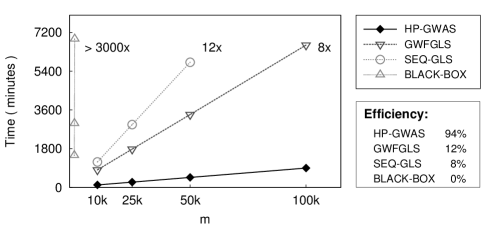
Figure 2: Comparison of the four presented algorithms for GWAS. The gain of each individual improvement from black-box to hp-gwas is illustrated. Additionally, our best algorithm, hp-gwas, outperforms state-of-the-art gwfgls by a factor of 8. All experiments were performed using a single thread. The other problem dimensions are: $n=10{,}000$, and $p=4$.

3.2 Results

Fig. 2 shows the timings of all four algorithms for an increasing value of $m$, the number of GLS problems to be solved. The experiments were run using a single thread. The results for black-box exemplify the limitations of solving a sequence of correlated problems as if they are unrelated: no matter how optimized the algorithm is for a single instance, it cannot compete with algorithms specially tailored to solve the sequence as a whole. As a first step towards high performance, seq-gls reuses computation across the sequence of problems. Consequently, the algorithm reduces dramatically the execution time of the naive black-box approach, leading to a speedup greater than 250.

hp-gwas further reduces the execution time of seq-gls by a factor of 12. The gain is explained by the effect of two optimizations. On the one hand, hp-gwas exploits application-specific knowledge, the structure of $X$, leading to a speedup of $p=4$ (larger values of $p$ result in even larger speedups). On the other hand, the computation is reorganized taking into account high-performance considerations. It is a common misconception that every BLAS routine attains the same efficiency. However, due to architectural constraints such as memory hierarchy and associated latency, BLAS-3 routines attain higher efficiency than BLAS-1 and BLAS-2. Therefore, rewriting multiple trsvs (BLAS-2) as a single large trsm (BLAS-3), our algorithm achieves an extra speedup of 3. As shown in Fig. 2, hp-gwas is an efficient algorithm to carry out GWAS; it attains 94% of the architecture’s peak performance.

Although gwfgls is aware of the specific properties of GWAS and benefits from such knowledge, the algorithm suffers from inefficiencies similar to seq-gls: it still performs redundant computation, and it is not properly tailored to benefit from BLAS-3 performance. The combination of both shortcomings results in a routine that is 8 times slower than hp-gwas.

Henceforth, we concentrate on hp-gwas and gwfgls. In Fig. 3 we report on the scalability of both algorithms. As the figure reflects, while gwfgls barely reaches a speedup of 2, completely stalling after 6 cores are used, hp-gwas attains a speedup of almost 11 when using 12 cores. Most interestingly, the tendency clearly shows that larger speedups are expected for hp-gwas when increasing the number of cores available.

The disparity in the scalability of these two algorithms is mainly due to their use of the BLAS library. In the case of gwfgls, the algorithm casts most of the computation in terms of the BLAS-2 operation gemv, which, being a memory-bound operation, is limited not only in performance but also in scalability. Instead, as described earlier, hp-gwas mainly builds on top of trsm (BLAS-3), which attains high scalability when operating on a large number of right-hand sides.

We provide in Fig. 4 timings for both algorithms when using 12 threads. As expected, the speedup of hp-gwas with respect to gwfgls soars from 8 to 50.

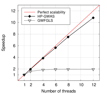
Figure 3: Scalability of hp-gwas and gwfgls. While gwfgls’ speedup plateaus at 2, and the gain is minimal for more than 4 cores, hp-gwas attains high-scalability and an even larger speedup is foreseen for a greater number of cores. The problem dimensions are: $n=10{,}000$, $p=4$, and $m=100{,}000$.

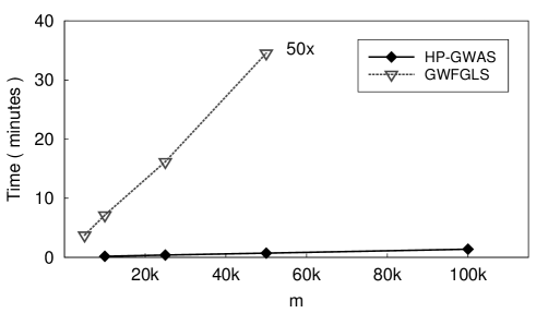
Figure 4: Timings for the multi-threaded versions of hp-gwas and gwfgls. Thanks to a much better scalability, our routine outperforms gwfgls by a factor of 50. The experiments were run using 12 threads. The other problem dimensions are: $n=10{,}000$, and $p=4$.

4 Out-of-core algorithm

So far, we have developed an algorithm for GWAS that overcomes the limitations of current approaches. It

1. solves a sequence of GLS problems,

2. exploits the available knowledge specific to GWAS, and

3. achieves high performance and scalability.

However, the algorithm presents a critical limitation: data must fit in main memory. The most common scenarios of GWAS require the processing of data sets that greatly exceed common main memory capacity: in a typical scenario, where 36 millions of GLS problems are to be solved with $n=10{,}000$, the size of the input operand $\mathcal{X}_{R}$ is roughly 3 terabytes. To overcome this limitation, we turn our attention to out-of-core algorithms [Toledo (1999)]. The goal is to design algorithms that make a proper use of available input/output (I/O) mechanisms to deal with data sets as large as the hard-drive size, while sustaining in-core high performance.

We regard the solution of GWAS as a process that takes as input a large stream of data, corresponding to successive GLS problems, and generates as output a large stream of data corresponding to the solution of such problems; thus, it demands out-of-core algorithms that efficiently stream data from secondary storage to main memory and vice versa.

We compare two approaches to data streaming. The first, used by GenABEL, is based on non-overlapping synchronous I/O; because of wait states, this approach introduces a considerable overhead in the execution time. The second, based on the well-known double-buffering technique, allows the overlapping of I/O with computation; thanks to the overlapping, wait states, and the associated overhead, are reduced or even completely eliminated.

Algorithm 7: Out-of-core algorithm for GWAS based on non-overlapping I/O

⬇

1$LL^{T}=M$ (potrf)

2$X_{L}:=L^{-1}X_{L}$ (trsm)

3$y:=L^{-1}y$ (trsv)

4$S_{TL}:=X_{L}^{T}X_{L}$ (syrk)

5$b_{T}:=X_{L}^{T}y$ (gemv)

6for each $X_{blk}$ in $\mathcal{X}_{R}$

7 read $(X_{blk})$

8 $X_{blk}:=L^{-1}X_{blk}$ (trsm)

9 for each $X_{R_{i}}$ in $X_{blk}$

10 $S_{BL_{i}}:=X_{R_{i}}^{T}X_{L}$ (gemv)

11 $S_{BR_{i}}:=X_{R_{i}}^{T}X_{R_{i}}$ (dot)

12 $b_{B_{i}}:=X_{R_{i}}^{T}y$ (dot)

13 $b_{i}:=S_{i}^{-1}b_{i}$ (posv)

14 write $(b_{blk})$

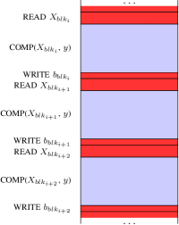
Figure 5: Non-overlapping approach to data streaming for out-of-core GWAS. I/O causes an overhead of 5% to 10%.

4.1 Non-overlapping approach

The application of non-overlapping synchronous I/O to our in-core algorithm (hp-gwas) results in Algorithm 7. The algorithm first computes the operations common to every GLS problem (lines 1 to 5) and then iterates over the stream of $X_{R}$’s (lines 6 to 14). At each iteration, the following actions are performed:

1. read the $X_{R}$’s for a block of successive GLS problems,

2. compute the solutions, $b$’s, of such problems, and

3. write the $b$’s to disk.

Both I/O requests (lines 7 and 14) are synchronous: after the requests are issued, the processor enters a wait state until the I/O transfer has completed. Fig. 5 depicts this shortcoming: red (dark) regions represent computation stalls where the processor waits for data to be read or written; blue (light) regions represent actual computation. Since loading data from secondary memory is orders of magnitude slower than loading data from main memory, I/O operations introduce a considerable overhead that negatively impacts performance. For the scenario described above, in which $n=10{,}000$, $p=4$, and $m=36{,}000{,}000$, synchronous I/O applied to hp-gwas causes a 5% to 10% overhead.

4.2 Overlapping approach - Double buffering

To put double buffering into practice, the main memory is split into two workspaces: one for downloading and uploading data and one for computation. Also, the data streams are divided into blocks such that they fit in the corresponding workspaces. While iterating over the blocks, the workspaces alternate their role, allowing the overlapping of I/O with computation, and reducing or even eliminating the overhead due to I/O. Specifically for GWAS, both workspaces are subdivided in individual buffers, one for each operand to be streamed, $\mathcal{X}_{R}$ and $b$. As illustrated in Fig. 6, at iteration $i$, results from the previous iteration are located in Workspace1::b and input data for next iteration is to be loaded in Workspace1::XR. Simultaneously, GLS problems corresponding to the current iteration $i$ are computed and stored in Workspace2::b. At iteration $i+1$ the workspaces exchange their role: Workspace1 is used for computation, and Workspace2 is used for I/O.

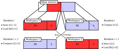
Figure 6: Workspaces for double buffering. The main memory is divided, from left to right, in global data, workspace 1, and workspace 2. Initially, workspace 1 is used for I/O and workspace 2 is used for computation. After each iteration, the workspaces exchange roles.

It remains to be addressed how the downloading and uploading of data is actually performed in the background while computation is being carried out. Our approach is based on the use of asynchronous libraries, which allow a process to request the prefetching of data needed for the next iteration: data is loaded in the background while the process carries out computation with the current data set.

In Algorithm 8 we provide the out-of-core algorithm ooc-hp-gwas that applies double-buffering to hp-gwas. At each iteration $i$ over the blocks of data (lines 6 to 16), the algorithm performs the following steps:

1. request the loading of the next block of input data (XR[i+1]),

2. wait, if necessary, for the current block of data (XR[i]),

3. compute the current set of problems defined by the current set of data,

4. request the storage of current results (b[i]), and

5. wait, if necessary, until previous results are stored (b[i-1]).

As illustrated in Fig. 7, a perfect overlapping of I/O with computation means that no I/O is exposed and no processor idles waiting for I/O operations.

Algorithm 8: Out-of-core algorithm for GWAS based on double-buffering

⬇

1$LL^{T}=M$ (potrf)

2$X_{L}:=L^{-1}X_{L}$ (trsm)

3$y:=L^{-1}y$ (trsv)

4$S_{TL}:=X_{L}^{T}X_{L}$ (syrk)

5$b_{T}:=X_{L}^{T}y$ (gemv)

6for each $X_{blk}$ in $\mathcal{X}_{R}$

7 async_read(next $X_{blk}$)

8 wait(current $X_{blk})$

9 $X_{blk}:=L^{-1}X_{blk}$ (trsm)

10 for each $X_{R_{i}}$ in $X_{blk}$

11 $S_{BL_{i}}:=X_{R_{i}}^{T}X_{L}$ (gemv)

12 $S_{BR_{i}}:=X_{R_{i}}^{T}X_{R_{i}}$ (dot)

13 $b_{B_{i}}:=X_{R_{i}}^{T}y$ (dot)

14 $b_{i}:=S_{i}^{-1}b_{i}$ (posv)

15 async_write(current $b_{blk}$)

16 wait(previous $b_{blk})$

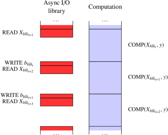
Figure 7: Overlapping approach to data streaming, based on an asynchronous library, for out-of-core GWAS. The figure depicts a perfect overlapping of I/O with computation.

4.3 Sustaining in-core high performance

A perfect overlapping is only one of two requirements for the out-of-core routine to sustain in-core high performance. The second is to ensure that the operations within the loop over the stream of data (lines 6 to 16) attain the same efficiency as in the in-core routine. Both requirements depend on the number of threads and the block size, i.e., the number of $X_{R}$’s loaded at each iteration.

To completely eliminate the overhead due to data movement from disk to memory and vice versa, the following equation must hold:

$${\tt time(computation)>time(load)+time(store)}.$$

The block size has to be large enough to ensure that for each iteration the time spent in computing is larger than the time spent on storing the previous results and loading data for the next iteration. Since the computation time varies with the number of threads, the block size needs to be adjusted accordingly.

Although it may seem that the best approach to select a block size is to simply maximize memory usage, the initial overhead must be taken into account: the loading of the first block of data is not overlapped with computation. In systems equipped with large amounts of main memory, it is advised to initiate the computation with a small block size to avoid exposed I/O, and increase it after a few iterations.

5 Performance results (II)

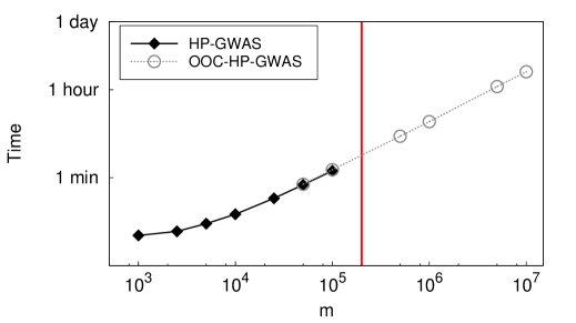
Figure 8: Our out-of-core routine, ooc-hp-gwas, sustains in-core performance for problems as large as the available secondary storage of 1 terabyte. The vertical line indicates the size limit for the in-core routine. The results were obtained using 12 threads. The other problem dimensions are: $n=10{,}000$, and $p=4$. We used a block size of $5{,}000$ throughout.

In this section, we focus on the experimental results for ooc-hp-gwas, our out-of-core routine. To measure the performance of the incorporated out-of-core mechanism, we compare the timings with those of the in-core routine, previously shown in Fig. 4. We complete the picture with a comparison between the timings of our routines and those of the in-core and out-of-core implementations of gwfgls. All routines were written in C, and the experiments were run in the same environment as Section 3. In addition, ooc-hp-gwas utilizes the AIO (asynchronous input/output) library, available on UNIX systems as part of their standard libraries.

In Fig. 8, we combine timings for both the in-core routine hp-gwas and the out-of-core routine ooc-hp-gwas. The in-core routine is used for problems whose data sets fit in main memory, and we switch to the out-of-core routine for larger problems. The vertical line indicates the size of the largest problem that can be solved in-core. The figure shows that, thanks to the double-buffering and an appropriate choice of the block size, ooc-hp-gwas achieves a perfect overlapping of I/O with computation. As a consequence, ooc-hp-gwas is able to sustain in-core performance for problems as large as the hard-drive size.

In Table 3, we collect timings for both our routines and gwfgls in both in-core and out-of-core scenarios. The provided ratios confirm the impact of using a sub-optimal approach to out-of-core: While, as seen in Fig. 8, the overlapping I/O mechanism incorporated in ooc-hp-gwas sustains in-core performance, the non-overlapping approach in gwfgls results in a 10% to 15% overhead. As a consequence, the speedup over gwfgls raises from 50 to 58.

$m=$	$10{,}000$	$50{,}000$	$100{,}000$	$500{,}000$	$1{,}000{,}000$	$5{,}000{,}000$	$10{,}000{,}000$
gwfgls	429.2	$2{,}072.5$	$4{,}117.9$	$24{,}065$	$48{,}130$	$240{,}650$	$481{,}300$
*hp-gwas	10.9	43.0	82.6	414	816	$4{,}184$	$8{,}343$
Ratio $\frac{\text{\sc gwfgls}}{\text{\sc*hp-gwas}}$	39.2	48.1	49.9	58.1	58.9	57.5	57.7

Table 3: Timings for gwfgls and *hp-gwas (hp-gwas and ooc-hp-gwas) for both in-core and out-of-core scenarios. The problem dimensions are: $n=10{,}000$ and $p=4$, for an increasing value of $m$. The results were obtained using 12 threads. The timings are in seconds. The double vertical line separates timings for the in-core (left) and out-of-core (right) routines. The increase in speedup in the out-of-core case reflects the overhead introduced in gwfgls due to a non-overlapping I/O.

The largest tests presented, involving 10 millions of genetic markers ($X_{R}$’s), took less than 2.5 hours with ooc-hp-gwas. This means that a complete genome-wide scan of association between 36 millions of genetic markers in a population of $10{,}000$ individuals takes now slightly more than 8 hours, and is only limited by the availability of a large (and cheap) secondary storage device.

6 Future Work

As current biomedical research experiences a large boost in the amount of available genomic data, computational biologists are eager to solve problems of ever increasing size. Even though the time spent to perform genome-wide analysis is reduced significantly thanks to the techniques presented in this paper, further speedups are required to satisfy future needs.

Throughout the paper we assumed, as is the case in current analyses, that the matrix $M$ fits in main memory. In this context, a further reduction of execution time can be achieved through distributed-memory architectures via an MPI parallelization: the processes would first perform the Cholesky factorization of $M$ redundantly, and then operate on distinct chunks of $X_{R}$. In addition, if GPUs with enough memory to host $M$ were available, the routines could be further sped up by offloading the computation of the trsm (line 8 in Alg. 8) onto the devices.

When instead $M$ does not fit in main memory, one should rely on approaches based on out-of-core algorithms-by-blocks [Quintana-Ortí et al. (2009), Quintana-Ortí et al. (2012)] and libraries such as ScaLAPACK [Blackford et al. (1997)] and Elemental [Poulson et al. (2012)], respectively for shared-memory and distributed-memory architectures.

7 Conclusions

We tackled a problem, extremely common in bioinformatics, that requires both high-performance computing and storage. Neither general nor domain-specific libraries provide a viable solution. Indeed, due to the expected execution time and storage requirements, it was believed that these problems could be solved exclusively with the aid of supercomputers. This paper instead demonstrates that a single multi-core node suffices.

We presented high-performance algorithms, and their corresponding implementations, for the solution of sequences of generalized least-squares problems (GLSs) in the context of genome-wide association studies (GWAS). When compared to the widely used gwfgls routine from the GenABEL package, our routines attain speedups larger than 50.

Our routines are specifically tailored for multi-threaded architectures. We followed an incremental approach: starting from an algorithm to solve one single GLS, we detailed the steps towards a high-performance algorithm for GWAS. At each step, we identified the limitations of current existing libraries and tools, and described the key insight to overcome such limitations.

First, we showed that no matter how optimized is a routine to solve a single GLS instance, it cannot possibly compete with tools specifically designed for GWAS: it is imperative to take advantage of the sequence of correlated problems. This discards the black-box approach of traditional libraries.

Then, we identified gwfgls’ issues regarding efficiency, scalability, and data handling, and detailed how we addressed them. Taking advantage of problem symmetries and application-specific knowledge, we were able to completely eliminate redundant computation. Next, we pointed out that even BLAS-3 kernels might suffer from low efficiency. A careful rearrangement of the operations leads to an efficiency of 94%. Combining two kinds of parallelism –a multi-threaded version of BLAS and OpenMP parallelism–, our in-core solver attains speedups close to 11 on 12 cores.

Finally, thanks to an adequate utilization of the double-buffering technique, allowing for a perfect overlapping of data transfers with computation, our out-of-core routine not only inherits in-core efficiency and scalability, but it is also capable of sustaining the achieved high performance for problems as large as the available secondary storage.

As an immediate result, our routines enable genome-wide association studies of unprecedented size and shift the limitation from computation time to size of secondary storage devices.

eceived Month Year; revised Month Year; accepted Month Year

References

- Anderson et al. (1999) Anderson, E., Bai, Z., Bischof, C., Blackford, S., Demmel, J., Dongarra, J., Du Croz, J., Greenbaum, A., Hammarling, S., McKenney, A., and Sorensen, D. 1999. LAPACK Users’ Guide, Third ed. Society for Industrial and Applied Mathematics, Philadelphia, PA.
- Antonio and Beirlant (2007) Antonio, K. and Beirlant, J. 2007. Actuarial statistics with generalized linear mixed models. Insurance: Mathematics and Economics 40, 1, 58 – 76.
- Aulchenko et al. (2010) Aulchenko, Y. S., Struchalin, M., and van Duijn, C. 2010. Probabel package for genome-wide association analysis of imputed data. BMC Bioinformatics 11, 1, 134.
- Blackford et al. (1997) Blackford, L. S., Choi, J., Cleary, A., D’Azevedo, E., Demmel, J., Dhillon, I., Dongarra, J., Hammarling, S., Henry, G., Petitet, A., Stanley, K., Walker, D., and Whaley, R. C. 1997. ScaLAPACK Users’ Guide. Society for Industrial and Applied Mathematics, Philadelphia, PA.
- Dongarra et al. (1990) Dongarra, J., Croz, J. D., Hammarling, S., and Duff, I. S. 1990. A set of level 3 basic linear algebra subprograms. ACM Trans. Math. Softw. 16, 1, 1–17.
- Gibbons et al. (2010) Gibbons, R. D., Hedeker, D., and DuToit, S. 2010. Advances in Analysis of Longitudinal Data. Annual Review of Clinical Psychology, vol. 6. ANNUAL REVIEWS, 4139 EL CAMINO WAY, PO BOX 10139, PALO ALTO, CA 94303-0897 USA, 79–107.
- Golub and Van Loan (1996) Golub, G. H. and Van Loan, C. F. 1996. Matrix computations (3rd ed.). Johns Hopkins University Press, Baltimore, MD, USA.
- (8) Hindorff, L., MacArthur, J., Wise, A., Junkins, H., Hall, P., Klemm, A., and Manolio, T. A catalog of published genome-wide association studies. Available at: www.genome.gov/gwastudies. Accessed July 22nd, 2012.
- Lauc et al. (2010) Lauc, G. et al. 2010. Genomics Meets Glycomics–The First GWAS Study of Human N-Glycome Identifies HNF1 as a Master Regulator of Plasma Protein Fucosylation. PLoS Genetics 6, 12 (12), e1001256.
- Levy et al. (2009) Levy, D. et al. 2009. Genome-wide association study of blood pressure and hypertension. Nature Genetics 41, 6 (Jun), 677–687.
- Poulson et al. (2012) Poulson, J., Marker, B., van de Geijn, R. A., Hammond, J. R., and Romero, N. A. 2012. Elemental: A new framework for distributed memory dense matrix computations. ACM Trans. Math. Softw.. To appear.
- Quintana-Ortí et al. (2012) Quintana-Ortí, G., Igual, F. D., Marqués, M., Quintana-Ortí, E. S., and Van de Geijn, R. A. 2012. A run-time system for programming out-of-core matrix algorithms-by-tiles on multithreaded architectures. ACM Transactions on Mathematical Software 38, 4.
- Quintana-Ortí et al. (2009) Quintana-Ortí, G., Quintana-Ortí, E. S., Van de Geijn, R. A., Van Zee, F. G., and Chan, E. 2009. Programming matrix algorithms-by-blocks for thread-level parallelism. ACM Trans. Math. Softw. 36, 3 (July), 14:1–14:26.
- Å. Björck (1996) Å. Björck. 1996. Numerical Methods for Least Squares Problems. SIAM, Philadelphia, USA.
- Speliotes et al. (2010) Speliotes, E. K. et al. 2010. Association analyses of 249,796 individuals reveal 18 new loci associated with body mass index. Nature Genetics 42, 11 (Nov), 937–948.
- Teslovich et al. (2010) Teslovich, T. M. et al. 2010. Biological, clinical and population relevance of 95 loci for blood lipids. Nature 466, 7307 (Aug), 707–713.
- Toledo (1999) Toledo, S. 1999. External memory algorithms. American Mathematical Society, Boston, MA, USA, Chapter A survey of out-of-core algorithms in numerical linear algebra, 161–179.