Blackbody radiation shift in the Sr optical atomic clock

Abstract

We evaluated the static and dynamic polarizabilities of the $5s^{2}~{}^{1}$S₀ and $5s5p~{}^{3}$P${}_{0}^{o}$ states of Sr using the high-precision relativistic configuration interaction + all-order method. Our calculation explains the discrepancy between the recent experimental $5s^{2}~{}^{1}$S${}_{0}-5s5p~{}^{3}$P${}_{0}^{o}$ dc Stark shift measurement $\Delta\alpha=247.374(7)$ [Middelmann et. al, arXiv:1208.2848 (2012)] and the earlier theoretical result of 261(4) a.u. [Porsev and Derevianko, Phys. Rev. A 74, 020502R (2006)]. Our present value of 247.5 a.u. is in excellent agreement with the experimental result. We also evaluated the dynamic correction to the BBR shift with 1% uncertainty; -0.1492(16) Hz. The dynamic correction to the BBR shift is unusually large in the case of Sr (7%) and it enters significantly into the uncertainty budget of the Sr optical lattice clock. We suggest future experiments that could further reduce the present uncertainties.

I Introduction

Optical lattice clocks have shown tremendous progress in recent years Swallows et al. (2012). An optical frequency standard based on the $5s^{2}~{}^{1}$S${}_{0}-5s5p~{}^{3}$P${}_{0}^{o}$ transition of ultracold ⁸⁷Sr atoms confined in a one-dimensional optical lattice is pursued by a number of groups Campbell et al. (2008); Ludlow et al. (2008); Falke et al. (2011); Baillard et al. (2008); Hong et al. (2009); Curtis et al. (2009). Its systematic uncertainty has been demonstrated at the 10^-16 fractional frequency level and an order-of-magnitude improvement is expected to be achieved soon Swallows et al. (2012); Falke et al. (2011). A three-dimensional optical lattice clock with bosonic ⁸⁸Sr was demonstrated for the first time in  Akatsuka et al. (2008).

The measured clock transition frequencies must be corrected in practice for the effect of the ambient blackbody radiation (BBR) shift, which is quite difficult to measure directly. The BBR shift can only be suppressed by cooling the clock. At room temperature, the differential BBR shift of the two levels of a clock transition turns out to make one of the largest irreducible contributions to the uncertainty budget of optical atomic clocks. The Sr clock transition has the largest BBR shift of all optical frequency standards that are currently under development (see Ref. Safronova et al. (2012) for a recent review). The fractional BBR shift ${\Delta\nu_{\rm BBR}}/{\nu_{0}}$ in Sr is more than a factor of 1000 larger than the fractional BBR shift in the Al⁺ ion clock Safronova et al. (2011). The BBR shift of an optical clock can generally be approximated by the dc Stark shift of the clock transition to about 1-2% precision, because optical frequencies are   100 times greater than characteristic BBR frequencies. However, Sr represents an exception, where the so-called dynamic correction Porsev and Derevianko (2006), that needs to be determined separately from the dc Stark shift, is 7%.

Table 1: Comparison of experimental Ral and theoretical energy levels of Sr in cm^-1. Two-electron binding energies are given in the first row, energies in other rows are given relative to the ground state. Results of the CI+MBPT and CI+all-order calculations are given in columns labeled “CI+MBPT” and “CI+All (A)”. The CI+all-order values with the ground state two-electron binding energy shifted by 200 cm^-1 are given in column labeled “CI+All (B)”. Corresponding relative differences of these three calculations with experiment are given in the three corresponding columns labeled “Diff.” in %. The $5s4d~{}^{3}$D${}_{1}-5s5p~{}^{3}$P${}_{0}^{o}$ transition energy is given in the last row.

State	Expt.	CI+MBPT	Diff.(%)	CI+All (A)	Diff.(%)	CI+All (B)	Diff.(%)
$5s^{2}~{}^{1}$S0	134897	136244	1.00	135444	0.41	135244	0.26
$5s4d~{}^{3}$D1	18159	18225	0.36	18327	0.93	18127	$-$0.18
$5s4d~{}^{3}$D2	18219	18298	0.44	18394	0.96	18194	$-$0.13
$5s4d~{}^{3}$D3	18319	18422	0.56	18506	1.02	18306	$-$0.07
$5s4d~{}^{1}$D2	20150	20428	1.38	20441	1.45	20241	0.45
$5s6s~{}^{3}$S1	29039	29369	1.14	29223	0.63	29023	$-$0.06
$5s6s~{}^{1}$S0	30592	30938	1.13	30777	0.61	30577	$-$0.05
$5s5d~{}^{1}$D2	34727	35092	1.05	34958	0.66	34758	0.09
$5s5d~{}^{3}$D1	35007	35371	1.04	35210	0.58	35010	0.01
$5s5d~{}^{3}$D2	35022	35388	1.04	35226	0.58	35026	0.01
$5s5d~{}^{3}$D3	35045	35412	1.05	35250	0.59	35050	0.01
$5p^{2}~{}^{3}$P0	35193	35854	1.88	35545	1.00	35345	0.43
$5p^{2}~{}^{3}$P1	35400	36070	1.89	35758	1.01	35558	0.45
$5p^{2}~{}^{3}$P2	35675	36344	1.88	36039	1.02	35839	0.46
$5s7s~{}^{3}$S1	37425	37776	0.94	37606	0.48	37406	$-$0.05
$5s6d~{}^{3}$D1	39686	40050	0.92	39876	0.48	39676	$-$0.02
$5s5p~{}^{3}$P${}_{0}^{o}$	14318	14806	3.41	14550	1.62	14350	0.23
$5s5p~{}^{3}$P${}_{1}^{o}$	14504	14995	3.38	14739	1.61	14539	0.24
$5s5p~{}^{3}$P${}_{2}^{o}$	14899	15399	3.36	15142	1.63	14942	0.29
$5s5p~{}^{1}$P${}_{1}^{o}$	21698	21955	1.18	21823	0.57	21623	$-$0.35
$4d5p~{}^{3}$F${}_{2}^{o}$	33267	33719	1.36	33648	1.14	33448	0.54
$4d5p~{}^{3}$F${}_{3}^{o}$	33590	34089	1.49	34003	1.23	33803	0.64
$4d5p~{}^{3}$F${}_{4}^{o}$	33919	34444	1.55	34347	1.26	34147	0.67
$4d5p~{}^{1}$D${}_{2}^{o}$	33827	34218	1.16	34208	1.13	34008	0.54
$5s6p~{}^{3}$P${}_{0}^{o}$	33853	34241	1.15	34055	0.59	33855	0.00
$5s6p~{}^{3}$P${}_{1}^{o}$	33868	34255	1.14	34071	0.60	33871	0.01
$5s6p~{}^{3}$P${}_{2}^{o}$	33973	34365	1.15	34134	0.47	33934	$-$0.12
$5s6p~{}^{1}$P${}_{1}^{o}$	34098	34476	1.11	34308	0.62	34108	0.03
3D${}_{1}-^{3}$P${}_{0}^{o}$	3842	3419	$-$11.0	3777	$-$1.69	3777	$-$1.69

Recently, the dc Stark shift in Sr has been measured with 0.003% precision  Middelmann et al. (2012), and the dynamic correction was evaluated based on a set of E1 transition rates and the Stark shift measurement. The measured value differed substantially (by almost $4\sigma$) from the previous theoretical determination  Porsev and Derevianko (2006).

In this work, we evaluate the static and dynamic polarizabilities of the $5s^{2}~{}^{1}$S₀ and $5s5p~{}^{3}$P${}_{0}^{o}$ states of Sr using the high-precision relativistic CI+all-order method. Our calculation explains the above-mentioned discrepancy between the experimental $5s^{2}~{}^{1}$S${}_{0}-5s5p~{}^{3}$P${}_{0}^{o}$ dc Stark shift measurement $\Delta\alpha=247.374(7)$ a.u. Middelmann et al. (2012) and the earlier theoretical result of 261(4) a.u. Porsev and Derevianko (2006). We found that the E1 matrix elements for the transitions that give dominant contributions to the ³P${}_{0}^{o}$ polarizability, in particular the $5s4d~{}^{3}$D${}_{1}-5s5p~{}^{3}$P${}_{0}^{o}$, are rather sensitive to the higher-order corrections to the wave functions and other corrections to the matrix elements beyond the random phase approximation. A correction of only 2.4% to the dominant ³D${}_{1}-^{3}$P${}_{0}^{o}$ matrix element leads to 5% difference in the final value of the ³P${}_{0}^{o}-\,^{1}$S₀ Stark shift. In this work, we included the higher-order corrections in an ab initio way using the CI+all-order approach, and also calculated several other corrections omitted in Porsev and Derevianko (2006). Our value for the dc Stark shift of the clock transition, 247.5 a.u., is in excellent agreement with the experimental result 247.374(7) a.u. Middelmann et al. (2012).

We have combined our theoretical calculations with the experimental measurements of the Stark shift Middelmann et al. (2012) and magic wavelength Ludlow et al. (2008) of the $5s^{2}~{}^{1}$S${}_{0}-5s5p~{}^{3}$P${}_{0}^{o}$ transition to infer recommended values of the several electric-dipole matrix elements that give the dominant contributions to the ³P${}_{0}^{o}$ polarizability. We used these values to evaluate the dynamic correction to the BBR shift of the ¹S${}_{0}-\,^{3}$P${}_{0}^{o}$ transition to be -0.1492(16) Hz.

We determined that the $5s4d~{}^{3}$D${}_{1}-5s5p~{}^{3}$P${}_{0}^{o}$ transition contributed 98.2% to the dynamic correction for the ³P${}_{0}^{o}$ level. Our calculation enables us to propose an approach for further reduction of the uncertainty in the BBR shift. In particular, there is a correlation in the uncertainty of the BBR shift and the lifetime of the $5s4d~{}^{3}$D₁ state, if branching ratios are known to sufficient accuracy. At present, experimental measurements of the $5s4d~{}^{3}$D term-averaged lifetime have an uncertainty of about 7% Miller et al. (1992); Redondo et al. (2004). We note that the experiment Miller et al. (1992), which was performed at JILA some 20 years ago, has relevance in the determination of the uncertainty budget of one of the world’s most accurate clocks now being developed at the same institution - a development probably not envisaged at the time.

A new determination of this (or ³D₁) lifetime with 0.5% uncertainty would provide a value of the Sr clock BBR shift that is accurate to about 0.5%, which would be a factor of 2 improvement in the uncertainty that we state here. This result is determined by the relevant branching ratios needed for the extraction of the $5s4d~{}^{3}$D${}_{1}-5s5p~{}^{3}$P${}_{0}^{o}$ matrix elements from the lifetime measurement. We have determined these branching ratios with an uncertainty of 0.2%. A further reduction in the uncertainty of the Sr clock BBR shift could be effected by an improved measurement of these branching ratios. The lifetime of the corresponding $6s5d~{}^{3}$D₁ state in Yb has been recently measured in Ref. Beloy et al. (2012).

Table 2: The CI+MBPT and CI+all-order results and further corrections to the E1 matrix elements for transitions that give dominant contributions to the polarizabilities of the $5s^{2}~{}^{1}$S₀ and $5s5p~{}^{3}$P${}_{0}^{o}$ states. The CI+MBPT and CI+all-order results including RPA corrections are given in columns labeled “MBPT+RPA” and “All+RPA”, respectively. The relative differences between the CI+all-order+RPA and CI+MBPT+RPA results are given in column “Higher orders” in %. The other contributions include the core-Brueckner ($\sigma$), two-particle (2P), structural radiation (SR), and normalization (Norm) corrections. Total relative size of corrections beyond CI+all-order+RPA is given in column “Corr.” in %. The recommended values for the $5s^{2}~{}^{1}$S${}_{0}-5s5p~{}^{1}$P${}_{1}^{o}$ matrix element was obtained from the ${}^{1}\!P_{1}^{o}$ lifetime measurement Yasuda et al. (2006), and the recommended values for all other transitions are from the present work (see Section V).

Transition	MBPT+RPA	All+RPA	Higher orders	2P	$\sigma$	SR	Norm	Final	Corr.(%)	Recomm.
$5s^{2}~{}^{1}$S${}_{0}-5s5p~{}^{1}$P${}_{1}^{o}$	5.253	5.272	$0.36\%$	$-0.006$	$0.004$	$0.032$	$-0.094$	$5.208$	$-1.23$	5.248(2)Yasuda et al. (2006)
$5s5p^{3}$P${}_{0}^{o}-5s4d~{}^{3}$D1	2.681	2.712	$1.14\%$	$-0.016$	$0.003$	$0.015$	$-0.048$	$2.667$	$-1.69$	2.675(13)
$5s5p^{3}$P${}_{0}^{o}-5s6s~{}^{3}$S1	1.983	1.970	$-0.66\%$	$0.002$	$-0.001$	$-0.006$	$-0.025$	$1.940$	$-1.55$	1.962(10)
$5s5p^{3}$P${}_{0}^{o}-5s5d~{}^{3}$D1	2.474	2.460	$-0.57\%$	$0.007$	$-0.001$	$-0.003$	$-0.031$	$2.432$	$-1.15$	2.450(24)
$5s5p^{3}$P${}_{0}^{o}-5p^{2}~{}^{3}$P1	2.587	2.619	$1.22\%$	$0.009$	$0.003$	$0.021$	$-0.033$	$2.620$	$0.04$	2.605(26)

II Method and energy levels

Calculation of Sr properties requires an accurate all-order treatment of electron correlations. This can be accomplished within the framework of the CI+all-order method that combines configuration interaction and coupled-cluster approaches Safronova et al. (2009, 2011); Porsev et al. (2012); Safronova et al. (2012, ). To evaluate uncertainties of the final results, we also carry out CI Kotochigova and Tupitsyn (1987) and CI+many-body perturbation theory (MBPT) Dzuba et al. (1996) calculations. These methods have been described in a number of papers Kotochigova and Tupitsyn (1987); Dzuba et al. (1996); Safronova et al. (2009, 2011) and we provide only a brief outline of these approaches.

We start with a solution of the Dirac-Fock (DF) equations

$$H_{0}\,\psi_{c}=\varepsilon_{c}\,\psi_{c},$$

where $H_{0}$ is the relativistic DF Hamiltonian Dzuba et al. (1996); Safronova et al. (2009) and $\psi_{c}$ and $\varepsilon_{c}$ are single-electron wave functions and energies. The calculations are carried out in the $V^{\rm{N-2}}$ potential. The wave functions and the low-lying energy levels are determined by solving the multiparticle relativistic equation for two valence electrons Kotochigova and Tupitsyn (1987),

$$H_{\rm eff}(E_{n})\Phi_{n}=E_{n}\Phi_{n}.$$

The effective Hamiltonian is defined as

$$H_{\rm eff}(E)=H_{\rm FC}+\Sigma(E),$$

where $H_{\rm FC}$ is the Hamiltonian in the frozen-core approximation. The energy-dependent operator $\Sigma(E)$ which takes into account virtual core excitations is constructed using second-order perturbation theory in the CI+MBPT method Dzuba et al. (1996) and using a linearized coupled-cluster single-double method in the CI+all-order approach Safronova et al. (2009). It is zero in a pure CI calculation. We refer the reader to Refs. Dzuba et al. (1996); Safronova et al. (2009) for detailed description of the construction of the effective Hamiltonian.

Unless stated otherwise, we use atomic units (a.u.) for all matrix elements and polarizabilities throughout this paper: the numerical values of the elementary charge, $|e|$, the reduced Planck constant, $\hbar=h/2\pi$, and the electron mass, $m_{e}$, are set equal to 1. The atomic unit for polarizability can be converted to SI units via $\alpha/h$ [Hz/(V/m)²]=2.48832$\times 10^{-8}\alpha$ (a.u.), where the conversion coefficient is $4\pi\epsilon_{0}a^{3}_{0}/h$ and the Planck constant $h$ is factored out in order to provide direct conversion into frequency units; $a_{0}$ is the Bohr radius and $\epsilon_{0}$ is the electric constant.

As a first test of the accuracy of our calculations, we compare our theoretical energies with experiment for a number of the even and odd parity states. Comparison of the energy levels (in cm^-1) obtained in the CI+MBPT, and CI+all-order approximations with experimental values Ral is given in Table 1. Ground state two-electron binding energies are given in the first row of Table 1, energies in other rows are measured from the ground state. The relative differences of the CI+MBPT and CI+all-order calculations with experiment (in %) are given in columns labeled “Diff”. Since the CI+all-order values are systematically higher than the experimental values, a large fraction of the difference from experiment can be attributed to the difference in the value of the ground state two-electron binding energy. We find that shifting the CI+all-order value of the ground state two-electron binding energy by only 200 cm^-1 (see results in column CI+all-order (B)) brings the results into excellent agreement with experiment for most of the states. We give the $5s4d~{}^{3}$D${}_{1}-5s5p~{}^{3}$P${}_{0}^{o}$ transition energy in the last row of Table 1. This transition is particulary important to the subject of this work, since it contributes 61% to the static polarizability and 98% to the dynamic correction to the BBR shift of the $5s5p~{}^{3}$P${}_{0}^{o}$ state. In fact, the accidentally small value of this transition energy is the source of the anomalously large (7%) dynamic correction to the BBR shift of the ${}^{1}\!S_{0}\rightarrow\,^{3}\!P^{o}_{0}$ transition in Sr. We see considerable improvement of the accuracy in this transition energy from the CI+MBPT to CI+all-order approximation, by a factor of 6. The CI+MBPT and CI+all-order values differs from the experiment by 11% and 1.7%, respectively.

Table 3: Contributions to the $5s^{2}\;{}^{1}$S₀ and $5s5p\;^{3}$P${}_{0}^{o}$ static polarizabilities of Sr in a.u. The dominant contributions to the valence polarizabilities are listed separately with the corresponding absolute values of electric-dipole reduced matrix elements given in columns labeled $D$. The theoretical and experimental Ral transition energies are given in columns $\Delta E_{\rm th}$ and $\Delta E_{\rm expt}$. The remaining contributions to valence polarizability are given in rows Other. The contributions from the core and $\alpha_{vc}$ terms are listed together in rows Core + Vc. The dominant contributions to $\alpha_{0}$, listed in columns $\alpha_{0}[\mathrm{A}]$ and $\alpha_{0}(\mathrm{B})$, are calculated with CI + all-order +RPA (no other corrections) matrix elements and theoretical [A] and experimental [B] energies Ral , respectively. The dominant contributions to $\alpha_{0}$ listed in column $\alpha_{0}[\mathrm{C}]$ are calculated with experimental energies and our final ab initio matrix elements. The dc Stark shift for the $5s5p~{}^{3}$P${}_{0}^{o}-5s^{2}~{}^{1}$S₀ transition is listed in the last rows of the table.

State	Contribution	$\Delta E_{\rm th}$	$\Delta E_{\rm expt}$	$D^{(a)}$	$\alpha_{0}[\mathrm{A}]$	$\alpha_{0}[\mathrm{B}]$	$D^{(b)}$	$\alpha_{0}[\mathrm{C}]$
$5s^{2}~{}^{1}$S0	$5s^{2}~{}^{1}$S${}_{0}-5s5p~{}^{1}$P${}_{1}^{o}$	21823	21698	5.272	186.4	187.4	5.208	182.9
	$5s^{2}~{}^{1}$S${}_{0}-5s5p~{}^{3}$P${}_{1}^{o}$	14739	14504	0.158	0.25	0.25		0.25
	$5s^{2}~{}^{1}$S${}_{0}-5s6p~{}^{1}$P${}_{1}^{o}$	34308	34098	0.281	0.34	0.34		0.34
	$5s^{2}~{}^{1}$S${}_{0}-4d5p~{}^{1}$P${}_{1}^{o}$	41242	41172	0.517	0.95	0.95		0.95
	Other				4.60	4.60		4.60
	Core + Vc				5.29	5.29		5.29
	Total				197.8	198.9		194.4
	Recomm.(c)							197.14(20)
$5s5p~{}^{3}$P${}_{0}^{o}$	$5s5p~{}^{3}$P${}_{0}-5s4d~{}^{3}$D1	3777	3842	2.712	285.0	280.2	2.667	270.9
	$5s5p~{}^{3}$P${}_{0}^{o}-5s6s~{}^{3}$S1	14673	14721	1.970	38.7	38.6	1.940	37.4
	$5s5p~{}^{3}$P${}_{0}^{o}-5s5d~{}^{3}$D1	20660	20689	2.460	42.9	42.8	2.432	41.8
	$5s5p~{}^{3}$P${}_{0}^{o}-5p^{2}~{}^{3}$P1	21208	21083	2.619	47.3	47.6	2.620	47.6
	$5s5p~{}^{3}$P${}_{0}^{o}-5s7s~{}^{3}$S1	23056	23107	0.516	1.69	1.69		1.69
	$5s5p~{}^{3}$P${}_{0}^{o}-5s6d~{}^{3}$D1	25326	25368	1.161	7.8	7.8		7.8
	Other				29.1	29.1		29.1
	Core +Vc				5.55	5.55		5.55
	Total				458.1	453.4		441.9
	Recomm.(d)							444.51(20)
3P${}_{0}^{o}-^{1}$S0					260.3	254.5		247.5
Theory Porsev and Derevianko (2006)					261(4)
Expt. Middelmann et al. (2012)								247.374(7)

^a CI+all-order+RPA values (no other corrections). ^b CI+all-order+RPA + other corrections. ^cObtained using experimental $5s5p~{}^{1}$P${}_{1}^{o}$ lifetime from Yasuda et al. (2006). ^dObtained using recommended value for the ¹S₀ polarizability and the experimental value of the Stark shift Middelmann et al. (2012).

III Ab initio calculation of electric-dipole matrix elements

The reduced electric-dipole matrix elements are obtained with the CI+all-order wave functions and effective electric-dipole operator $D_{\rm eff}$ in the random-phase approximation (RPA). The effective operator accounts for the core-valence correlations in analogy with the effective Hamiltonian Dzuba et al. (1998); Por . We include additional corrections beyond RPA in the calculation of the E1 matrix elements in comparison with  Porsev and Derevianko (2006); Porsev et al. (2008). These contributions include the core-Brueckner ($\sigma$), two-particle (2P) corrections, structural radiation (SR), and normalization (Norm) corrections Dzuba et al. (1998); Por . While we find some cancelation between the various corrections, these cannot be omitted at the 1% level of accuracy. Partial cancelation of the structural radiation and normalization corrections was discussed in Ref. Dzuba et al. (1987). Detailed analysis of the structure radiation correction was carried out in the same work  Dzuba et al. (1987).

The results for several transitions that give dominant contributions to the ¹S${}_{0}-^{3}$P${}_{0}^{o}$ dc Stark shift are summarized in Table 2. The percentage differences between the CI+all-order+RPA and CI+MBPT+RPA calculations are given in the column labeled “Higher orders”. We note that it is positive for some transitions and negative for other transitions. Our final ab initio values are given in column labeled “Final”. We find that total relative size of corrections beyond CI+all+RPA given in column labeled “Corr” is small, 0.04-1.7%, but significant. We estimate the uncertainties in the ab initio values of the matrix elements to be 1% based on the comparison of the CI+MBPT+RPA and CI+all-order+RPA values and combined size of other corrections.

We also provide the recommended values for these transitions. The recommended value for the $5s^{2}~{}^{1}$S${}_{0}-5s5p~{}^{1}$P${}_{1}^{o}$ matrix element was obtained in Porsev and Derevianko (2006); Porsev et al. (2008) from the ${}^{1}\!P_{1}^{o}$ lifetime measurement from photoassociation spectra Yasuda et al. (2006), the recommended values for all other transitions are obtained in the present work in Section V.

IV Polarizabilities

We evaluated the static and dynamic polarizabilities of the $5s^{2}~{}^{1}$S₀ and $5s5p~{}^{3}$P${}_{0}^{o}$ states of Sr using the high-precision relativistic CI+all-order method. The scalar polarizability $\alpha_{0}(\omega)$ is separated into a valence polarizability $\alpha_{0}^{v}(\omega)$, ionic core polarizability $\alpha_{c}$, and a small term $\alpha_{vc}$ that modifies ionic core polarizability due to the presence of two valence electrons. The valence part of the polarizability is determined by solving the inhomogeneous equation in valence space, which is approximated as Kozlov and Porsev (1999)

$$(E_{v}-H_{\textrm{eff}})|\Psi(v,M^{\prime})\rangle=D_{\textrm{eff}}|\Psi_{0}(v,J,M)\rangle$$ (1)

for the state $v$ with total angular momentum $J$ and projection $M$. The wave function $\Psi(v,M^{\prime})$ is composed of parts that have angular momenta of $J^{\prime}=J,J\pm 1$ that allows us to determine the scalar and tensor polarizability of the state $|v,J,M\rangle$ Kozlov and Porsev (1999). The effective dipole operator $D_{\textrm{eff}}$ includes RPA corrections. The core and $\alpha_{vc}$ terms are evaluated in the random-phase approximation. Their uncertainty is determined by comparing the DF and RPA values. The small $\alpha_{vc}$ term is calculated by adding $\alpha_{vc}$ contributions from the individual electrons, i.e. $\alpha_{vc}(5s^{2})=2\alpha_{vc}(5s)$, and $\alpha_{vc}(5s5p)=\alpha_{vc}(5s)+\alpha_{vc}(5p)$. The frequency dependence of the core and $\alpha_{vc}$ terms is negligible, and we use their static values in all calculations.

Table 4: Breakdown of the contributions to the $5s5p\;^{3}$P${}_{0}^{o}$ static polarizability $\alpha_{0}(\omega=0)$ and dynamic polarizability $\alpha_{0}(\omega)$ at the 813.4 nm magic wavelength. The dominant contributions to the valence polarizabilities are obtained with experimental energies and recommended values of the matrix elements. The electric-dipole reduced matrix elements are given in column labeled “$D^{\rm recom}$”. The experimental Ral transition energies are given in column labeled “$\Delta E_{\rm expt}$”. The remaining contributions to valence polarizability are given in row labeled “Other”. The contributions from the core and $\alpha_{vc}$ terms are listed together in row labeled “Core + Vc”.

Contribution	$\Delta E_{\rm expt}$	$D^{\rm recom}$	$\alpha_{0}(\omega)$	$\alpha_{0}(\omega=0)$
$5s5p~{}^{3}$P${}_{0}^{o}-5s4d~{}^{3}$D1	3842	2.675(13)	-29.5	272.6(3.3)
$5s5p~{}^{3}$P${}_{0}^{o}-5s6s~{}^{3}$S1	14721	1.962(10)	126.4	38.3(4)
$5s5p~{}^{3}$P${}_{0}^{o}-5s5d~{}^{3}$D1	20689	2.450(24)	65.6	42.5(8)
$5s5p~{}^{3}$P${}_{0}^{o}-5p^{2}~{}^{3}$P1	21083	2.605(26)	71.4	47.1(9)
$5s5p~{}^{3}$P${}_{0}^{o}-5s7s~{}^{3}$S1	23107	0.516(8)	2.4	1.69(5)
$5s5p~{}^{3}$P${}_{0}^{o}-5s6d~{}^{3}$D1	25368	1.161(17)	10.2	7.8(2)
Other			34.1	29.1(9)
Core + Vc			5.55	5.55(6)
Total			286.0	444.5

While we do not use the sum-over-states approach in the calculation of the polarizabilities, it is important to establish the dominant contributions to the final values. We combine the electric-dipole matrix elements and energies according to the sum-over-states formula for the valence polarizability Mitroy et al. (2010):

$$\alpha_{0}^{v}(\omega)=\frac{2}{3(2J+1)}\sum_{n}\frac{(E_{n}-E_{v})|\langle v\|D\|n\rangle|^{2}}{(E_{n}-E_{v})^{2}-\omega^{2}}$$ (2)

to calculate the contributions of specific transitions. Here, $J$ is the total angular momentum of the state $v$, $D$ is the electric-dipole operator, $E_{i}$ is the energy of the state $i$, and frequency $\omega$ is zero in the static polarizability calculations.

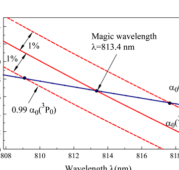
Figure 1: (Color online) The frequency-dependent polarizabilities of the Sr $5s^{2}~{}^{1}$S₀ and $5s5p~{}^{3}$P${}_{0}^{o}$ states near 813.4 nm magic wavelength. The frequency-dependent polarizability of $5s5p~{}^{3}$P${}_{0}^{o}$ shifted by $\pm$ 1% are shown to illustrate the sensitivity of the magic wavelength to the $5s5p~{}^{3}$P${}_{0}^{o}$ polarizability. The magic wavelength is marked with arrow.

Table 5: Dynamic corrections to the BBR shift of the $5s^{2}~{}^{1}$S${}_{0}-5s5p\;^{3}$P${}^{o}_{0}$ clock transition in Sr at $T=300~{}K$ (in Hz). Quantities $\eta_{i}$, $\Delta E_{g}^{\rm dyn}$, and $\Delta\nu_{{}^{3}\!P_{0}^{o}-^{1}\!S_{0}}^{\rm dyn}$ are defined in text.

	$\eta_{1}$	$\eta_{2}$	$\eta_{3}$	$\eta$	$\alpha_{0}(\omega=0)$	$\Delta E_{g}^{\rm dyn}/h$
Total $(5s^{2}~{}^{1}$S${}_{0})$	0.00163	0.00001	0	0.00164	197.1	-0.0028
$5s5p~{}^{3}$P${}_{0}^{o}-5s4d~{}^{3}$D1	0.03394	0.00414	0.00088	0.03896
$5s5p~{}^{3}$P${}_{0}^{o}-5s6s~{}^{3}$S1	0.00032	0	0	0.00032
$5s5p~{}^{3}$P${}_{0}^{o}-5s5d~{}^{3}$D1	0.00018	0	0	0.00018
$5s5p~{}^{3}$P${}_{0}^{o}-5p^{2}~{}^{3}$P1	0.00019	0	0	0.00020
$5s5p~{}^{3}$P${}_{0}^{o}-5s7s~{}^{3}$S1	0.00001	0	0	0.00001
$5s5p~{}^{3}$P${}_{0}^{o}-5s6d~{}^{3}$D1	0.00002	0	0	0.00002
Total $(5s5p~{}^{3}$P${}_{0}^{o})$	0.03467	0.00415	0.00088	0.03970	444.6	-0.1520
Final $\Delta\nu_{{}^{3}\!P_{0}^{o}-^{1}\!S_{0}}^{\rm dyn}$						-0.1492(16)
Ref. Middelmann et al. (2012)						-0.1477(23)

We have carried out several calculations of the dominant contributions to the polarizabilities using different sets of the energies and E1 matrix elements in order to understand the difference of the theoretical predictions for the Stark shift $5s^{2}~{}^{1}\!S_{0}-5s5p~{}^{3}\!P^{o}_{0}$ $\Delta\alpha=261(4)~{}$a.u. and recent experimental measurement $\Delta\alpha=247.374(7)$ a.u. as well as to provide a recommended value for the $5s5p~{}^{3}$P${}_{0}^{o}-5s4d~{}^{3}$D₁ matrix element. The results are summarized in Table 3. Other theoretical calculations of Sr polarizabilities were recently compiled in review Mitroy et al. (2010). The ground-state polarizability of Sr was calculated using relativistic coupled-cluster (RCC) method in Sahoo and Das (2008). Their value 199.7(7.3) a.u. is in agreement with our calculations.

In Table 3 the absolute values of the corresponding reduced electric-dipole matrix elements are listed in columns labeled “$D$” in a.u.. The theoretical and experimental Ral transition energies are given in columns $\Delta E_{\rm th}$ and $\Delta E_{\rm expt}$. The remaining valence contributions are given in rows labeled “Other”. The contributions from the core and $\alpha_{vc}$ terms are listed together in row labeled “Core +Vc”. The dominant contributions to $\alpha_{0}$ listed in columns $\alpha_{0}[\mathrm{A}]$ and $\alpha_{0}[\mathrm{B}]$ are calculated with CI + all-order +RPA (no other corrections) matrix elements and theoretical [A] and experimental [B] energies Ral , respectively.

Our $\alpha_{0}[\mathrm{A}]$ result agrees with the earlier calculation of  Porsev and Derevianko (2006) which was carried out using CI+MBPT approach with energy fitting that approximated missing higher-order corrections to the wave functions. We note that this may be fortuitous since the calculation of  Porsev and Derevianko (2006) was carried out in $V^{N}$ potential, while we are using $V^{N-2}$ potential since the present version of the CI+all-order method is formulated for $V^{N-2}$ potential. The E1 matrix elements in Porsev and Derevianko (2006); Porsev et al. (2008) included RPA but omitted all other corrections calculated in the present work. We find that replacing the theoretical energies with experimental values reduces the Stark shift by 2.3%. We note that in the case of Sr all of the states contributing to the polarizabilities are included in our computational basis and this procedure is not expected to cause problems with basis set completeness, as in the case of Yb  Dzuba and Derevianko (2010). The dominant contributions to $\alpha_{0}$ listed in column $\alpha_{0}[\mathrm{C}]$ are calculated with experimental energies and final ab initio matrix elements. Inclusion of the small corrections further reduces the value of the Stark shift by 3.1%, and our resulting value obtained with our final ab initio matrix elements is in excellent agreement with experiment Middelmann et al. (2012).

V Determination of recommended values of electric-dipole matrix elements

To further improve our values of the other matrix elements, we use the measurement of the magic wavelength for the ³P${}_{0}^{o}-^{1}$S₀ clock transition to determine recommended values of the $5s5p~{}^{3}$P${}_{0}^{o}-5s6s~{}^{3}$S₁, $5s5p~{}^{3}$P${}_{0}^{o}-5s5d~{}^{3}$D₁, and $5s5p~{}^{3}$P${}_{0}^{o}-5p^{2}~{}^{3}$P₁ matrix elements. The ¹S₀ polarizability at the 813.4 nm magic wavelength is 286.0 a.u. which is essentially fixed by the value of the $5s5p~{}^{1}$P${}_{1}^{o}$ lifetime  Porsev et al. (2008). The contributions to the ³P${}_{0}^{o}$ polarizability at the magic wavelength are listed in Table 4. Since the contribution of the $5s5p~{}^{3}$P${}_{0}^{o}-5s6s~{}^{3}$S₁ transition is dominant, the magic wavelength limits the value of this matrix element within about 0.5%. Since we appear to systematically overestimate the correction to matrix elements beyond CI+all+RPA approximation, we adjust the values of two other $5s5p~{}^{3}$P${}_{0}^{o}-5s5d~{}^{3}$D₁ and $5s5p~{}^{3}$P${}_{0}^{o}-5p^{2}~{}^{3}$P₁ matrix elements in a similar way as the $5s5p~{}^{3}$P${}_{0}^{o}-5s6s~{}^{3}$S₁ one. We plot the dynamic polarizabilities of the ¹S₀ and ³P${}_{0}^{o}$ states in the vicinity of the magic wavelength on Fig. 1 to illustrate that the crossing point is extremely sensitive to the matrix element values. The 0.5% change in the values of the matrix elements (corresponding to 1% change in the value of the ${}^{3}\!P_{0}^{o}$ polarizability) shifts the crossing point by more than 4 nm.

Table 6: Experimental transition energies (in cm^-1), theoretical line strengths (in a.u.), transition rates (in s^-1), and branching ratios for transitions contributing to the $5s4d\ ^{3}$D_J lifetimes. The CI+RPA, CI+MBPT+RPA, and CI+all-order+RPA results are listed in columns labeled “CI”, “MBPT”, and “All”, respectively. The recommended values of the $\langle 5s5p\ ^{3}$P${}^{o}_{1,2}||D||5s4d\ ^{3}$D${}_{1,2}\rangle|$ and $|\langle 5s5p\ ^{3}$P${}^{o}_{2}||D||5s4d\ ^{3}$D${}_{3}\rangle|$ matrix elements are obtained using the recommended matrix element for the $5s4d\ ^{3}$D${}_{1}\rightarrow 5s5p\ ^{3}$P${}^{o}_{0}$ transition (i.e. scaled by 0.9862). Experimental energies are used in all cases. Numbers in square brackets represent powers of 10.

Transition	$\Delta E_{\rm epxt}$	Line strengths $S$				Transition rates $A_{ab}$			Branching ratios
		CI	MBPT	All	Recomm.	MBPT	All	Recomm.	CI	MBPT	All
3D${}_{1}\rightarrow\,^{3}$P${}_{0}^{o}$	3842	9.503	7.189	7.357	7.156	2.753[5]	2.817[5]	2.740[5]	0.5949	0.5954	0.5953
3D${}_{1}\rightarrow\,^{3}$P${}_{1}^{o}$	3655	7.172	5.414	5.543	5.391	1.785[5]	1.828[5]	1.777[5]	0.3866	0.3861	0.3862
3D${}_{1}\rightarrow\,^{3}$P${}_{2}^{o}$	3260	0.485	0.365	0.374	0.364	8.541[3]	8.750[3]	8.510[3]	0.0186	0.0185	0.0185
$\sum_{b\leq a}{A_{ab}}$						4.623[5]	4.722[5]	4.602[5]
3D${}_{2}\rightarrow\,^{3}$P${}_{1}^{o}$	3714			16.605	16.149		3.448[5]	3.354[5]			0.8058
3D${}_{2}\rightarrow\,^{3}$P${}_{2}^{o}$	3320			5.602	5.449		0.831[5]	0.808[5]			0.1942
$\sum_{b\leq a}{A_{ab}}$							4.279[5]	4.162[5]
3D${}_{3}\rightarrow\,^{3}$P${}_{2}^{o}$	3421			31.519	30.655		3.652[5]	3.552[5]

Table 7: The lifetimes of the $5s4d~{}^{3}$D_J states in ns. The last three rows give term-averaged ³D lifetime.

	MBPT	All	Recomm.
$\tau(5s4d~{}^{3}$D${}_{1})$	2163	2113	2171(24)
$\tau(5s4d~{}^{3}$D${}_{2})$		2337	2403(27)
$\tau(5s4d~{}^{3}$D${}_{3})$		2738	2816(31)
$\tau(5s4d~{}^{3}$D$)$		2453	2522(28)
Expt. Miller et al. (1992)		2900(200)
Expt. Redondo et al. (2004)		2500(200)

After we determined the values of these three matrix elements, we used them to obtain the value of the $5s5p~{}^{3}$P${}_{0}^{o}-5s4d~{}^{3}$D₁ matrix element from the experimental value of the Stark shift. We determine its uncertainty from the uncertainty of all the other contributions to the ³P${}_{0}^{o}$ polarizability value (listed in the last column of Table 4). Since our theoretical values may experience a systematic shift in one direction, we (somewhat conservatively) simply add all of the uncertainties, totaling to $3.3$ a.u, instead of adding them in quadrature. Assigning this value to be the uncertainty in the dominant ${}^{3}\!D_{1}$ contribution of 272.7 a.u., we estimate the uncertainty in the recommended value of the $5s5p~{}^{3}$P${}_{0}^{o}-5s4d~{}^{3}$D₁ matrix element to be 0.5%. Since the contributions to both static and dynamic polarizabilities from $5s5p~{}^{3}$P${}_{0}^{o}-5s7s~{}^{3}$S₁ and $5s5p~{}^{3}$P${}_{0}^{o}-5s6d~{}^{3}$D₁ transitions are small, we use ab initio CI+all+RPA values and assign them 1.5% uncertainty. Combined with experimental energies and other small contributions, the set of recommended matrix elements reproduces recommended values for both the $5s5p~{}^{3}$P${}_{0}^{o}$ static and dynamic polarizability at 813.4 nm magic wavelength.

VI Blackbody radiation shift

The leading contribution to the multipolar black body radiation (BBR) shift of the energy level $g$ can be expressed in terms of the electric dipole transition matrix elements Farley and Wing (1981)

$$\Delta E_{g}=-\frac{(\alpha k_{B}T)^{3}}{2J_{g}+1}\sum_{n}|\langle g||D||n\rangle|^{2}F_{1}(y_{n}).$$ (3)

Here $k_{B}$ is the Boltzmann constant, $y_{n}\equiv(E_{n}-E_{g})/(k_{B}T)$, and $F_{1}(y)$ is the function introduced by Farley and Wing in Farley and Wing (1981). Its asymptotic expansion is given by

$$F_{1}\left(y\right)\approx\frac{4\pi^{3}}{45y}+\frac{32\pi^{5}}{189y^{3}}+\frac{32\pi^{7}}{45y^{5}}+\frac{512\pi^{9}}{99y^{7}}.$$ (4)

The Eq. (3) can be expressed in terms of the dc polarizability $\alpha_{g}(\omega=0)$ of the state $g$ as Porsev and Derevianko (2006)

$$\Delta E_{g}=-\frac{2}{15}(\alpha\pi)^{3}(k_{B}T)^{4}\alpha_{g}(0)+\Delta E_{g}^{\rm dyn}.$$ (5)

Here $\Delta E_{g}^{\rm dyn}$ is determined as

$$\Delta E^{\rm dyn}_{g}\equiv-\frac{2}{15}(\alpha\pi)^{3}(k_{B}T)^{4}\alpha_{g}(0)\,\eta$$ (6)

and $\eta$ represents a “dynamic” fractional correction to the total shift that reflects the averaging of the frequency dependence of the polarizability over the frequency of the blackbody radiation spectrum. Corresponding shift in the clock transition frequency, $\Delta\nu_{{}^{3}\!{\rm P}_{0}^{o}-^{1}\!S_{0}}^{\rm dyn}=(\Delta E^{\rm dyn}_{{}^{3}\!P_{0}^{o}}-\Delta E^{\rm dyn}_{{}^{1}\!S_{0}})/h$, is referred to as dynamic correction to the BBR shift. The quantity $\eta$ can be approximated by Porsev and Derevianko (2006)

$$\eta=\eta_{1}+\eta_{2}+\eta_{3}=\frac{80}{63\,(2J_{g}+1)}\,\frac{\pi^{2}}{\alpha_{g}(0)k_{B}T}$$

$$\times\sum_{n}\frac{|\langle n||D||g\rangle|^{2}}{y_{n}^{3}}\left(1+\frac{21\pi^{2}}{5\,y_{n}^{2}}+\frac{336\pi^{4}}{11y_{n}^{4}}\right).$$ (7)

Dynamic corrections to the BBR shift of the $5s^{2}~{}^{1}$S${}_{0}-5s5p\;^{3}$P${}_{0}^{o}$ clock transition in Sr at $T=300~{}K$ (in Hz) are given in Table 5. The dynamic correction to the BBR shift of the ³P${}_{0}^{o}$ level is dominated by the contribution from the $5s5p~{}^{3}$P${}_{0}^{o}-5s4d~{}^{3}$D₁ transition, which contributes 98.2% of the total. Our final result $-0.1492(16)$ Hz is in excellent agreement with recent value $-0.1477(23)$ Hz of Ref. Middelmann et al. (2012).

Our result enables us to propose an approach for further reduction of the uncertainty in the BBR shift: a measurement of the $5s4d~{}^{3}$D₁ lifetime with 0.5% uncertainty would provide the value of the BBR shift in Sr clock that is accurate to about 0.5%, which would be a factor of 2 improvement in the uncertainty stated here. Such a determination assumes accurate knowledge of the branching ratios.

The $5s4d~{}^{3}$D₁ level decays to all three $5s5p~{}^{3}$P${}_{0,1,2}^{o}$ states, but the branching ratio to the ³P${}_{2}^{o}$ level is very small. The lifetime of a state $a$ is calculated as

$$\tau_{a}=\frac{1}{\sum_{b\leq a}A_{ab}}.$$

The E1 transition rates $A_{ab}$ are calculated using

$$A_{ab}=\frac{2.02613\times 10^{18}}{\lambda^{3}}\frac{S}{2J_{a}+1}{\rm s}^{-1},$$

where $\lambda$ is the wavelength of the transition in $\AA$ and $S$ is the line strength.

We find that the branching ratios are essentially independent of the correlation corrections to the matrix elements. We note that line strength ratios are close to the non-relativistic ones (5/9, 5/12, 1/36), with the differences being $-$0.23%, +0.22%, and 1.4% for the ³D${}_{1}-^{3}$P_J transitions, respectively. We illustrate this point in Table 6, where we list the relevant energies, line strengths $S$, transition rates $A$, and branching ratios in the CI, CI+MBPT, and CI+all-order approximations.

The RPA corrections to the matrix elements are included in all cases. We used experimental energies in all calculations for consistency. We find that the difference in the CI, CI+MBPT, and CI+all-order branching ratio results is less than 0.1%. Since all the other corrections are small, their uncertainties should be even smaller. As a result, the accuracy of our branching ratios should be better than 0.2%. The recommended values for the $5s5p\ ^{3}$P${}_{1,2}^{o}-5s4d\ ^{3}$D₁ matrix elements are obtained using the recommended matrix element for the $5s5p\ ^{3}$P${}_{0}^{o}-5s4d\ ^{3}$D₁ transition and CI+all-order branching ratios. The recommended values for the transition rates and the $5s4d\ ^{3}$D₁ lifetime, 2172(24) ns, are obtained using the recommended values of the matrix elements and experimental energies. We also list the recommended values ³D₂, ³D₃, and term-averaged ³D lifetimes in Table 7. The ³D term-averaged lifetime is compared with experiment Miller et al. (1992); Redondo et al. (2004).

VII Conclusion

We have evaluated the static and dynamic polarizabilities of the $5s^{2}~{}^{1}$S₀ and $5s5p~{}^{3}$P${}_{0}^{o}$ states of Sr and explained the discrepancy between the recent experimental $5s^{2}~{}^{1}$S${}_{0}-5s5p~{}^{3}$P${}_{0}^{o}$ dc Stark shift measurement  Middelmann et al. (2012) and the earlier theoretical result Porsev and Derevianko (2006). Our theoretical value for the dc Stark shift of the clock transition, 247.5 a.u., is in excellent agreement with the experimental result. We have provided the recommended values of the matrix elements for transitions that give dominant contributions to the clock Stark shift and evaluated their uncertainties. We evaluated the dynamic correction to the BBR shift of the ¹S${}_{0}-\,^{3}$P${}_{0}^{o}$ clock transition at $300~{}K$ to be -0.1492(16) Hz and proposed an approach for further reduction of the uncertainty in the BBR shift.

References

- Swallows et al. (2012) M. D. Swallows, M. J. Martin, M. Bishof, C. Benko, Y. Lin, S. Blatt, A. M. Rey, and J. Ye, IEEE Transactions on Ultrasonics, Ferroelectrics, and Frequency Control 59, 416 (2012).
- Campbell et al. (2008) G. K. Campbell, A. D. Ludlow, S. Blatt, J. W. Thomsen, M. J. Martin, M. H. G. de Miranda, T. Zelevinsky, M. M. Boyd, J. Ye, S. A. Diddams, et al., Metrologia 45, 539 (2008).
- Ludlow et al. (2008) A. D. Ludlow, T. Zelevinsky, G. K. Campbell, S. Blatt, M. M. Boyd, M. H. G. de Miranda, M. J. Martin, J. W. Thomsen, S. M. Foreman, J. Ye, et al., Science 319, 1805 (2008).
- Falke et al. (2011) S. Falke, H. Schnatz, J. S. R. Vellore Winfred, T. Middelmann, S. Vogt, S. Weyers, B. Lipphardt, G. Grosche, F. Riehle, U. Sterr, et al., Metrologia 48, 399 (2011).
- Baillard et al. (2008) X. Baillard, M. Fouché, R. Le Targat, P. G. Westergaard, A. Lecallier, F. Chapelet, M. Abgrall, G. D. Rovera, P. Laurent, P. Rosenbusch, et al., E. Phys. J. D 48, 11 (2008).
- Hong et al. (2009) F.-L. Hong, M. Musha, M. Takamoto, H. Inaba, S. Yanagimachi, A. Takamizawa, K. Watabe, T. Ikegami, M. Imae, Y. Fujii, et al., Opt. Lett. 34, 692 (2009).
- Curtis et al. (2009) E. A. Curtis, Y. B. Ovchinnikov, I. R. Hill, G. P. Barwood, and P. Gill, in Frequency Standards and Metrology, edited by L. Maleki (2009), pp. 218–222.
- Akatsuka et al. (2008) T. Akatsuka, M. Takamoto, and H. Katori, Nat. Phys. 4, 954 (2008).
- Safronova et al. (2012) M. S. Safronova, M. G. Kozlov, and C. W. Clark, IEEE Transactions on Ultrasonics, Ferroelectrics, and Frequency Control 59, 439 (2012).
- Safronova et al. (2011) M. S. Safronova, M. G. Kozlov, and C. W. Clark, Phys. Rev. Lett. 107, 143006 (2011).
- Porsev and Derevianko (2006) S. G. Porsev and A. Derevianko, Phys. Rev. A 74, 020502(R) (2006).
- (12) Yu. Ralchenko, A. Kramida, J. Reader, and the NIST ASD Team (2011). NIST Atomic Spectra Database (version 4.1). Available at http://physics.nist.gov/asd. National Institute of Standards and Technology, Gaithersburg, MD.
- Middelmann et al. (2012) T. Middelmann, S. Falke, C. Lisdat, and U. Sterr, ArXiv e-prints (2012), eprint 1208.2848.
- Redondo et al. (2004) C. Redondo, M. Sanchezrayo, P. Ecija, D. Husain, and F. Castano, Chem. Phys. Lett. 392, 116 (2004).
- Miller et al. (1992) D. A. Miller, L. Yu, J. Cooper, and A. Gallagher, Phys. Rev. A 46, 062516 (1992).
- Beloy et al. (2012) K. Beloy, J. A. Sherman, N. D. Lemke, N. Hinkley, C. W. Oates, and A. D. Ludlow, ArXiv e-prints (2012), eprint 1208.0552.
- Yasuda et al. (2006) M. Yasuda, T. Kishimoto, M. Takamoto, , and H. Katori, Phys. Rev. A 73, 011403R (2006).
- Safronova et al. (2009) M. S. Safronova, M. G. Kozlov, W. R. Johnson, and D. Jiang, Phys. Rev. A 80, 012516 (2009).
- Porsev et al. (2012) S. G. Porsev, M. S. Safronova, and M. G. Kozlov, Phys. Rev. Lett. 108, 173001 (2012).
- Safronova et al. (2012) M. S. Safronova, S. G. Porsev, M. G. Kozlov, and C. W. Clark, Phys. Rev. A 85, 052506 (2012).
- (21) M. S. Safronova, S. G. Porsev, and C. W. Clark, arXiv:1208.1456, Phys. Rev. Lett (2012), in press.
- Kotochigova and Tupitsyn (1987) S. A. Kotochigova and I. I. Tupitsyn, J. Phys. B 20, 4759 (1987).
- Dzuba et al. (1996) V. A. Dzuba, V. V. Flambaum, and M. G. Kozlov, Phys. Rev. A 54, 3948 (1996).
- Dzuba et al. (1998) V. A. Dzuba, M. G. Kozlov, S. G. Porsev, and V. V. Flambaum, JETP 87, 885 (1998).
- (25) S. G. Porsev, Yu. G. Rakhlina, and M. G.Kozlov, Phys. Rev. A 60 2781 (1999); J. Phys. B 32, 1113 (1999).
- Porsev et al. (2008) S. G. Porsev, A. D. Ludlow, M. M. Boyd, and J. Ye, Phys. Rev. A 78, 032508 (2008).
- Dzuba et al. (1987) V. A. Dzuba, V. V. Flambaum, P. G. Silvestrov, and O. P. Sushkov, J. Phys. B 20, 1399 (1987).
- Kozlov and Porsev (1999) M. G. Kozlov and S. G. Porsev, Eur. Phys. J. D 5, 59 (1999).
- Mitroy et al. (2010) J. Mitroy, M. S. Safronova, and C. W. Clark, J. Phys. B 43, 202001 (2010).
- Sahoo and Das (2008) B. K. Sahoo and B. P. Das, Phys. Rev. A 77, 062516 (2008).
- Dzuba and Derevianko (2010) V. A. Dzuba and A. Derevianko, J. Phys. B 43, 074011 (2010).
- Farley and Wing (1981) J. W. Farley and W. H. Wing, Phys. Rev. A 23, 2397 (1981).