Rotational periods and evolutionary models for subgiant stars observed by CoRoT

Abstract

Context. We present rotation period measurements for subgiants observed by CoRoT. Interpreting the modulation of stellar light that is caused by star-spots on the time scale of the rotational period depends on knowing the fundamental stellar parameters.

Aims. Constraints on the angular momentum distribution can be extracted from the true stellar rotational period. By using models with an internal angular momentum distribution and comparing these with measurements of rotation periods of subgiant stars we investigate the agreement between theoretical predictions and observational results. With this comparison we can also reduce the global stellar parameter space compatible with the rotational period measurements from subgiant light curves. We can prove that an evolution assuming solid body rotation is incompatible with the direct measurement of the rotational periods of subgiant stars.

Methods. Measuring the rotation periods relies on two different periodogram procedures, the Lomb-Scargle algorithm and the Plavchan periodogram. Angular momentum evolution models were computed to give us the expected rotation periods for subgiants, which we compared with measured rotational periods.

Results. We find evidence of a sinusoidal signal that is compatible in terms of both phase and amplitude with rotational modulation. Rotation periods were directly measured from light curves for 30 subgiant stars and indicate a range of 30 to 100 d for their rotational periods.

Conclusions. Our models reproduce the rotational periods obtained from CoRoT light curves. These new measurements of rotation periods and stellar models probe the non-rigid rotation of subgiant stars. .

1 Introduction

For the first time in modern astrophysics, two space missions, Kepler and CoRoT, are providing accurate observations of solar-like oscillations for hundreds of main-sequence stars and thousands of red giant stars (Baglin et al. 2006; Borucki et al. 2009). CoRoT observes in the direction of the intersection between the equator and the Galactic plane. In each of these fields, CoRoT has identified many solar-type dwarf stars (Baglin et al. 2006). Another abundant class observed by CoRoT are giant stars. Intermediate between these two groups are the subgiants, a known rare class of objects. They have been accepted as an explicit stellar group in 1930 (Strömberg 1930). Until the 1950s they were not understood in terms of stellar evolution theory. An interesting review of the subgiant history can be found in Sandage et al. (2003). Theoretically, when stars exhaust their hydrogen in the core (turn-off), they leave the main sequence (MS), pass through the subgiant phase and become red giants. Studying subgiants is interesting for several reasons: they are particularly appropriate for dating purposes (Thorén et al. 2004), are associated with rotation periods ($P_{\mathrm{rot}}$), and can be useful in stellar gyrochronology. F-type subgiants are important for studying solar-like oscillations (Barban & Michel 2006). As stars evolve through the subgiant branch, their surface convection zone becomes deeper. The matter that resided below the surface convection zone at the MS is then exposed. From the subgiant phase to the red giant branch, the stellar radius increases at the same time that the convection zone deepens. It is the first dredge-up.

The rotation period of subgiant stars could constrain the interior angular momentum distribution and mixing in low-mass stars. Subgiant $P_{\mathrm{rot}}$ measurements can teach us about the rotation of low-mass stars and by implication about the solar rotation as well. Subgiants are more evolved and slightly more luminous than the Sun. They are expected to rotate with $P_{\mathrm{rot}}$ greater than the $P_{\mathrm{rot}}^{\odot}$. Many of them have a convective core. The deepening of the convective layers has a major influence on the chemical abundance and chromospheric activity in this phase (do Nascimento et al. 2000, 2003 and references therein). Studies show that lithium abundance in subgiants agrees well with dilution predictions and reflects the well-known dilution process that occurs when the convective envelope deepens after turn-off (Iben 1967; do Nascimento et al. 2000). On the other hand, more massive cool subgiant stars show lithium depletion by up to two orders of magnitude before the start of dilution. The de Medeiros et al. (1997); Lèbre et al. (1999); do Nascimento et al. (2000) and Palacios et al. (2003) results agree with the findings by Balachandran (1990) and Burkhart & Coupry (1991) about a few slightly evolved field subgiants that originate from the hot side of the dip and show significant lithium depletion. As suggested by Vauclair (1991) and Charbonnel & Vauclair (1992), the additional lithium depletion from rotationally

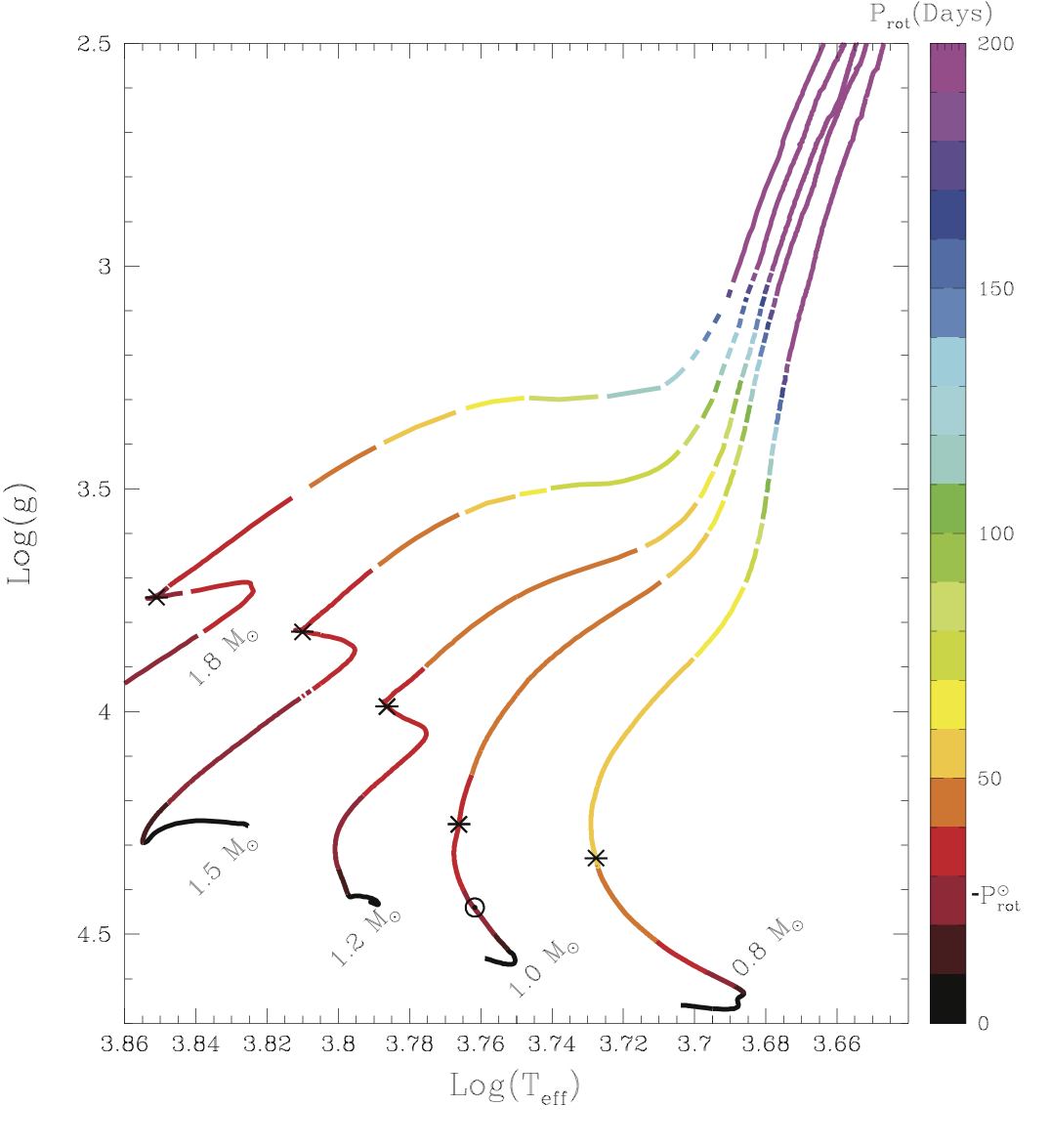
Figure 1: $Log(g)-T_{{\rm eff}}$ diagram. Evolutionary models for [Fe/H] = 0.0 and for 0.8, 1.0, 1.2, 1.5, and 1.8 solar masses. The color pallet denotes the evolution of rotation period for each model. The Sun is flagged and the beginning of the subgiant branch (turn-off point) is marked with an asterisk.

induced mixing (Charbonnel & Vauclair 1992; Charbonnel & Talon 1999) occurs early inside these stars when they are on the MS, even if its signature does not appear at the stellar surface at the age of the Hyades. This extra-mixing process is linked to rotation. If the Sun rotates as a solid body, it should have a $P_{\mathrm{rot}}$ greater than 90 d when it will become a subgiant. The Pinsonneault et al. (1989) non standard models for subgiants imply a $P_{\mathrm{rot}}$ of 50 d for subgiants. Clearly, a directly measured rotation period is needed to decide in this matter. Until now, the only available $P_{\mathrm{rot}}$ for subgiants were inferred from chromospheric activity calibrations (Noyes et al. 1984) and are a matter of debate. We aim to give a quantitative answer based on direct measurements of $P_{\mathrm{rot}}$ for selected CoRoT subgiants.

In this study we measured $P_{\mathrm{rot}}$ for a sample of subgiants and present updated evolutionary models with an internal distribution of angular momentum to probe the expected $P_{\mathrm{rot}}$ for the subgiant branch. We organize the paper as follows: we describe the observational sample and the $P_{\mathrm{rot}}$ determination in Sect. 2. The models are presented in Sect.  3. The results are discussed in Sect. 4. We summarize our conclusions in Sect. 5.

2 Stellar sample and time series analysis

The focus of our study is a first analysis of the $P_{\mathrm{rot}}$ for selected subgiants observed by CoRoT. For the instrument description and its operation readers are referred to Auvergne et al. (2009). We used the available public data level 2 (N2) light curves that are ready for scientific analysis. These light curves were delivered by the CoRoT pipeline after nominal corrections (Samadi et al. 2006). In the present analysis we used stars classified as subgiants by Gazzano et al. (2010). We chose only light curves with $\sim 150$ d with a low contamination factor and high-quality photometry without systematic errors. Eventual discontinuities and long-term trends were corrected following a similar procedure as in Affer et al. (2012).

2.1 Time series analysis

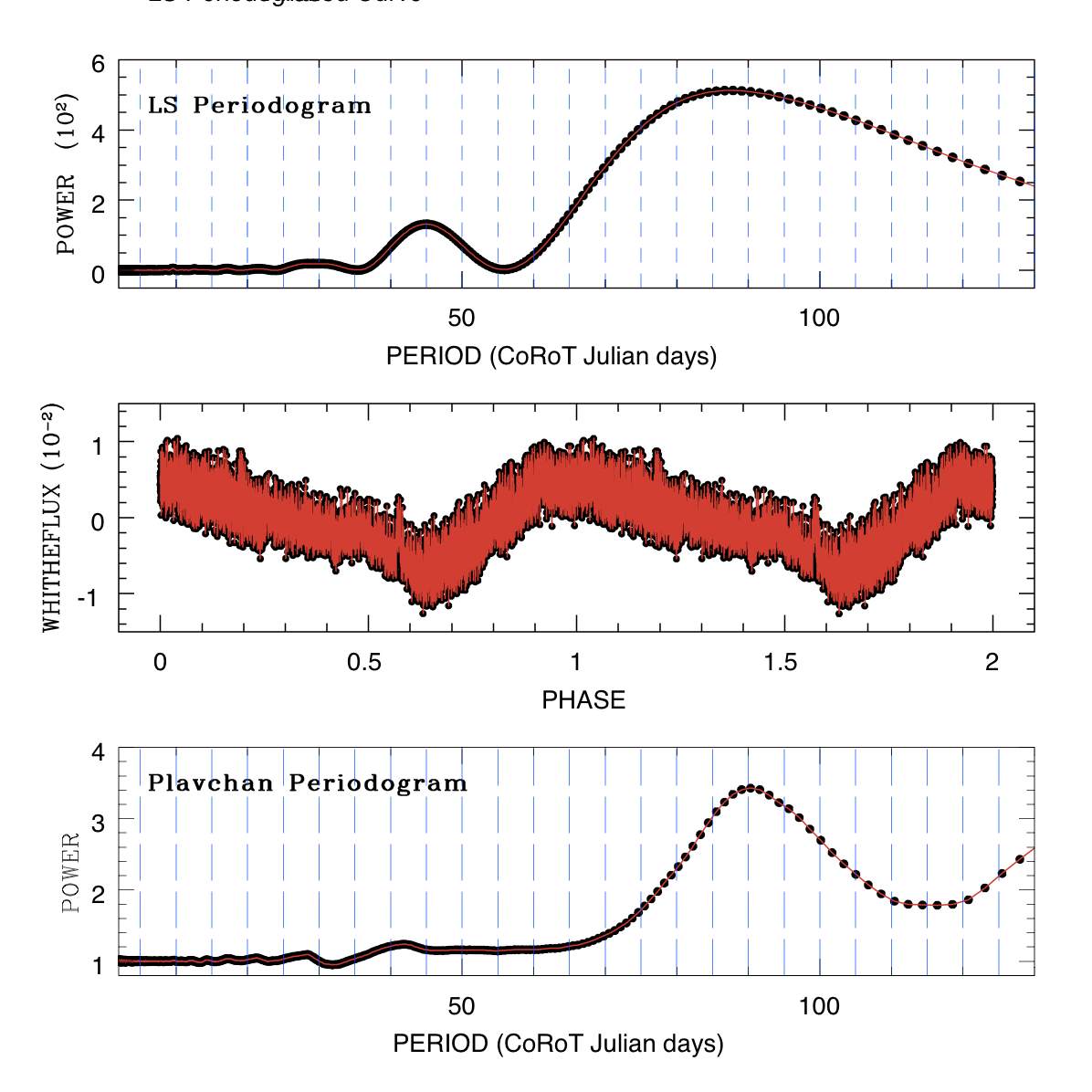
Figure 2: CoRoT ID 100570829. In the top panel we show the LS periodogram with the $P_{\mathrm{rot}}=84.2$ d derived with the LS algorithm. In the middle panel we show the phased curve for this $P_{\mathrm{rot}}$. In the bottom panel we show the Plavchan periodogram.

To achieve the largest possible sample of subgiants with determined $P_{\mathrm{rot}}$, stars analyzed by Gazzano et al. (2010) that are in the CoRoT Exo-Dat database were checked for periodic modulation. To determine the rotational periods for our sample of subgiants, we used a combination of two procedures, the Lomb-Scargle (LS) algorithm (Scargle 1982), and the Plavchan periodogram (Plavchan et al. 2008). For time series in which the sampling is not uniformly distributed, the LS periodogram analysis is particularly suitable. The LS algorithm identifies sinusoidal periodic signals in time series such as pulsating variable stars. The Plavchan algorithm is a variant of the phase dispersion minimization (PDM) algorithm (Stellingwerf 1978) that does not use phase bins. It competently detects periodic time series shapes that are poorly described by the assumptions of other algorithms. This procedure is more computationally demanding than the LS analysis.

For each star, we applied the two procedures and then isolated the most significant periods of each method. For the LS algorithm, we computed the normalized power as a function of periods and then searched for peaks in the function. To decide whether there is a significant signal from a certain period in the power spectrum, the power at that period was linked to the false-alarm probability (FAP). This is the probability that a peak with a power z equal to, or higher than, the highest peak observed in the periodogram would appear anywhere in the considered frequency range in the presence of pure noise. We derived the FAP for all detected periods and only those with an FAP $<$ 0.000001 were considered as significant peaks. The FAP is given by $FAP=1-[1-exp(-z)]^{N_{i}}$, where $N_{i}=-6.362+1.193N+0.00098N^{2}$ is the number of independent frequencies, $N$ is the number of data points and $z$ the height of the peak (e.g., Horne & Baliunas 1986). For clumped data, Scholz & Eislöffel (2004) used $N_{i}$ = N / 2 for their first estimation of an FAP. These two different approaches do not result in a significant change of the FAP. The light curve coverage allows us to detect periods longer than 2 d and shorter than 100 d with a relevant FAP $<$ 0.000001. The uncertainties in $P_{\mathrm{rot}}$ are determined by the frequency resolution in the power spectrum and the sampling error. The error of our measurement is defined by the probable error, which in turn is defined as 0.2865$\cdot$FWHM (full-width at half-maximum of the peak), assuming a Gaussian statistics around the LS peak. The most significant periods are compared with models presented in Sect. 3. Our final work sample is composed of 30 subgiant stars. The derived periods and their respective errors are presented in Table LABEL:gen_table. In Fig. 2 we show the Lomb-Scargle periodogram (top), the phased curve (middle), and the Plavchan periodogram (bottom) for CoRoT ID 100570829. This is a representative subgiant star classified as a K0IV in the Exo-Dat (Deleuil et al. 2006, 2009; Meunier et al. 2007) and Gazzano et al. (2010). The data we used were obtained during the CoRoT first long run (LRc01 and LRa01). The rotation periods for this target were derived from Lomb-Scargle and Plavchan periodograms analysis of the light curve, giving $P_{\mathrm{rot}}=84.2\leavevmode\nobreak\ \pm$ 15.8 d with a FWHM of 55 d. The $P_{\mathrm{rot}}$ uncertainty comes mainly from the time series limitation.

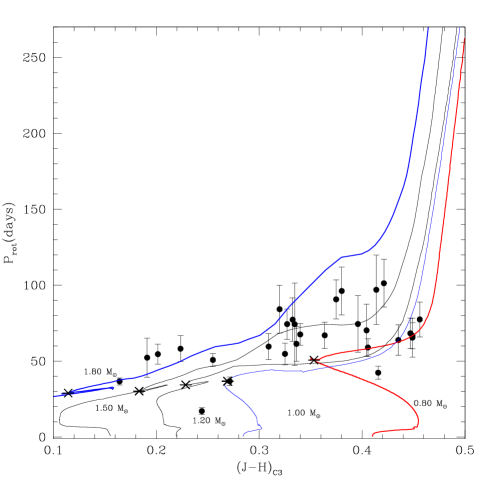
Figure 3: Rotation period evolution from the main sequence to the giant branch as a function of (J – H)_C3 index. The models are shown for [Fe/H] = 0 and different stellar masses computed with differential rotation. Filled circles stand for rotational periods determined as described in the Sect. 2. The beginning of the subgiant branch (turn-off point) is flagged with an asterisk.

Figure 4: Rotation period evolution from the main sequence to the giant branch as a function of the (J – H)_C3 index. The models are shown for [Fe/H] = 0 and 1 M_⊙. The dashed line represents the rotation period evolution for a solid-body model. The solid line represents the computed model with differential rotation. Open circles represent subgiants with masses of about one solar mass and rotational periods determined from the rotation-activity relation by Lovis et al. (2011). Asterisk as in Fig 3.

3 Evolutionary models

Our models were computed with the Toulouse-Geneva stellar evolution code (Hui-Bon-Hoa 2008). More details of the physics used in the models can be found in Richard et al. (1996, 2004), Hui-Bon-Hoa (2008), and do Nascimento et al. (2009) as well as in Appendix A . The initial composition follows the Grevesse & Noels (1993) mixture. The convection was treated according to the Böhm-Vitense (1958) formalism of the mixing length theory with a mixing length parameter $\alpha=l/H_{\mathrm{p}}$, where $l$ is the mixing length and $H_{\mathrm{p}}$ the pressure height scale. The rotation-induced mixing due to meridional circulation and the transport of angular momentum due to rotationally induced instabilities are computed as described by Zahn (1992) and Talon & Zahn (1997) and takes into account differential rotation. The angular momentum distribution at a given time is a function of its previous history. As underlined by Pinsonneault et al. (1989), the initial conditions are critical for rotating models. The angular momentum loss from the disk-locking process is linked with stellar magnetic fields and remains poorly understood. The evolution of the angular momentum is computed with the Kawaler (1988) prescription as in equation 1. Our solar model is calibrated to match the observed solar effective temperature, luminosity, and rotation at the solar age. The calibration is based on the Richard et al. (1996) prescription. For a 1.0 $M_{\odot}$ star, we adjusted the mixing-length parameter $\alpha$ and the initial helium abundance $Y_{\mathrm{ini}}$ to reproduce the observed solar luminosity, and the radius at the solar age: $L_{\odot}=3.8515\pm 0.0055\times 10^{33}\ \mathrm{erg\cdot s^{-1}}$, $R_{\odot}=6.95749\pm 0.00241\times 10^{10}\ \mathrm{cm}$, and $t_{\odot}=4.57\pm 0.02\ \mathrm{Gyr}$ (Richard et al. 2004). For the best-fit solar model, we obtained $L=3.8514\times 10^{33}\ \mathrm{erg\cdot s^{-1}}$ and $R=6.95750\times 10^{10}\ \mathrm{cm}$ at an age $t=4.576\ \mathrm{Gyr}$, with ${Y_{\mathrm{ini}}=0.277}$ and ${\alpha=1.72}$. The free parameters of the rotation-induced mixing determine the efficiency of the turbulent motions and are adjusted to produce a mixing that satisfies both the helium gradient below the surface convective zone, which improves the agreement between the model and seismic sound speed profiles, and the absence of beryllium destruction (see Appendix A for details. We used the initial angular momentum inferred by Pinsonneault et al. (1989) for the Sun $J_{0}=1.63\times 10^{50}\mathrm{\leavevmode\nobreak\ g\cdot cm^{2}\cdot s^{-1}}$ and calibrated the angular momentum loss by requiring that the solar model has the solar rotation rate at the solar age. We obtained the solar surface rotation velocity $v=2.2\mathrm{\leavevmode\nobreak\ km\cdot s^{-1}}$ at the solar age. The models of 0.8, 1.0, 1.2, 1.5, and 1.8 solar masses (Fig. 1) were computed from the zero-age main sequence (ZAMS) to the top of the red giant branch (RGB) with the same calibration values as for the solar model. In these diagrams the asterisk indicates the evolutionary region where the subgiant branch starts, this point corresponds to the age of hydrogen exhaustion in stellar central regions. From Alonso et al. (1999) we calibrated $T_{{\rm eff}}$ as function of (J – H) color index. For the selected objects we obtained (J – H) 2MASS photometry from CoRoT Exo-Dat and applied the pseudo-colors $C_{3}$ reddening correction as described by Catelan et al. (2011) to obtain the reddening-free index (J – H)_C3.

4 Results

The $P_{\mathrm{rot}}$ measured from light curves for subgiants are shown in Fig. 3. These $P_{\mathrm{rot}}$ measurements indicate the range of 30 to 100 d for subgiants in agreement with expected $P_{\mathrm{rot}}$ from models. The $P_{\mathrm{rot}}$ for subgiants with $M<1.80\leavevmode\nobreak\ M_{\odot}$ increases slightly until the bottom of the RGB. Fig. 4 compares the expected $P_{\mathrm{rot}}$ from a 1.00 $M_{\odot}$ model rotating as a solid body with a 1.00 $M_{\odot}$ rotating differentially. Open circles represent $P_{\mathrm{rot}}$ for subgiants determined by Lovis et al. (2011). Our models follow the same prescription for the angular momentum loss as Pinsonneault et al. (1989) and an updated physics (opacities, equation of state, meridional circulation, and shear instabilities). The metallicity effect on the evolution of the rotational period for models with $[Fe/H]=\pm 0.3\leavevmode\nobreak\ dex$ is lower than the LS intrinsical error. On the subgiant branch, the separations of solid-body rotation models and models with internal angular momentum distribution are satisfactorily distinguished by the measured rotation periods from CoRoT light curves. Thus, we emphasize that this range of rotation periods for subgiants reinforces the scene of a strong radial differential rotation in depth at the main sequence or a fast core rotating in the subgiant branch. The $P_{\mathrm{rot}}$ in the subgiant phase is driven by the deepening of the convective zone, which extracts angular momentum from the radial differential rotation reservoir. From the angular momentum conservation, this extraction compensates for the increase of the momentum of inertia due to the stellar radius enhancement. It causes the difference between the two models shown in Fig. 4. Another interesting fact is that subgiants present a chromospheric activity lower than main-sequence stars with the same mass (Lovis et al. 2011), even if its convective zone is deeper than their progenitor. This scenario contrasts with the suggestion of the magnetic breaking as the root cause of the low rotation of subgiants (Gray & Nagar 1985).

5 Conclusion

We have reported $P_{\mathrm{rot}}$ for 30 subgiants observed by CoRoT. These $P_{\mathrm{rot}}$ combined with evolutionary models helped us to more tightly constrain the angular momentum evolution for evolved stars, which is inaccessible to direct observations. Our $P_{\mathrm{rot}}$ agree well with the range of periods determined from the activity modulation studies of subgiants. We showed that subgiants present $P_{\mathrm{rot}}$ ranging from 30 to 100 d in the mass range from 0.8 to 1.8 solar masses. This work presents a first step in addressing the study of the $P_{\mathrm{rot}}$ of the subgiants. Our models agree with rotational period measurements for subgiant stars. The rotation period range for subgiants reinforces the scene of a differential rotation in depth or a fast-core rotating. This result also agrees with the findings by Mosser et al. (2012) who observed that rotational splittings and core rotation significantly slows down during the RGB.

Appendix A Description of the physics adopted for the transport of internal angular momentum

In addition to the input described in Sect. 3., we provide here more details on the physics adopted for the transport of internal angular momentum for the present modeling. We used the same approach as Pinsonneault et al. (1989) after updating the treatment of the instabilities relevant to the transport of angular momentum according to Zahn (1992) and Talon & Zahn (1997).

Initial conditions: The rotational properties are strongly influenced by the pre-main-sequence phase. Kawaler (1987) determined the initial angular momentum for the Sun as $J_{0}=1.63\times 10^{50}\ \mathrm{g\cdot cm^{2}\cdot s^{-1}}$.

Angular momentum loss: Kawaler (1988) described the angular momentum loss for stars with an outer convective envelope as

$$\frac{dJ}{dt}=-K\Omega^{1+4N/3}\left(\frac{R}{R_{\odot}}\right)^{2-N}\left(\frac{M}{M_{\odot}}\right)^{-N/3},$$ (1)

with $\Omega$ the angular velocity and $K$ a constant that combines scale factors for the wind velocity and magnetic field strength. This is adjusted to give the solar surface rotation velocity at the solar age. $N$ denotes the wind index and is a measure of the magnetic geometry. $N=3/2$ for the Sun. The mass loss dependence rate is very weak, and we assumed the rate $\dot{M}$ to be $10^{-14}\ M_{\odot}\cdot\mathrm{yr^{-1}}$.

Transport of matter and angular momentum: The redistribution of matter and angular momentum is carried out by dynamical instabilities (convection and dynamical shear mainly) that occur on a time scale much shorter than the evolutionary time scale, and also by secular instabilities (Eddington circulation and secular shear) with a similar or longer time scale. The Eddington meridional circulation (Eddington 1926), is a large-scale mass motion due to thermic gradients caused by rotation. The vertical velocity $U_{\mathrm{r}}$ of this circulation is related to the divergence of the radiation flux (Eddington 1925; Sweet 1950; Zahn 1987). In a uniformly rotating star, $U_{\mathrm{r}}$ has the following analytical form:

$$U_{r}=\frac{8}{3}\frac{\Omega^{2}r^{5}}{G^{2}}\frac{L}{M^{3}}\frac{\nabla_{\mathrm{ad}}}{\nabla_{\mathrm{ad}}-\nabla_{\mathrm{rad}}}\left(1-\frac{\Omega^{2}}{2\pi G\rho}\right)P_{2}(\cos\theta),$$ (2)

where $\Omega$ is the angular velocity, $r$ the mean radius, and $\rho$ the density of the considered equipotential, $L$ and $M$ are the luminosity and the mass at this location, $G$ is the gravitational constant, $\nabla_{\mathrm{ad}}$ and $\nabla_{\mathrm{rad}}$ are the adiabatic and radiative gradients; $P_{2}(\cos\theta)$ is the second-order Legendre polynomial in which $\theta$ is the colatitude. This flow advects angular momentum and thereby induces differential rotation.

The rotation state is then a result from the balance between meridional advection and turbulent stresses. Shear instabilities ensure that the angular velocity is constant in equipotential surfaces. The turbulent viscosity is assumed to be anisotropic and dominant in the horizontal over the vertical direction. Horizontal turbulent motions work against the advection of chemicals by the meridian flow, which homogenizes horizontal layers. The vertical transport of matter is accordingly treated as a diffusion process:

$$\rho\frac{\partial\bar{c}}{\partial t}=\frac{1}{r^{2}}\frac{\partial}{\partial r}\left(r^{2}\rho D_{turb}\frac{\partial\bar{c}}{\partial r}\right),$$ (3)

with $\rho$ being the density, $r$ the radial coordinate, $\bar{c}$ the mean concentration diffusing vertically, and

$D_{turb}=D_{v}+\frac{[rU_{r}(r)]^{2}}{30D_{h}}$

the turbulent diffusion coefficient expressed from the vertical and horizontal diffusion coefficients, valid when $D_{h}\gg D_{v}$. $U_{r}(r)$ is the amplitude of the vertical component of the circulation velocity. If we assume that the meridional velocity and the turbulent diffusion coefficients are correlated (Zahn 1992), we have

$D_{turb}=\alpha_{turb}r|U_{r}|$, with $\alpha_{turb}=C_{v}+\frac{1}{30C_{h}}$.

The free parameters $\alpha_{turb}$ and $C_{h}$ are adjusted in our models to reproduce the solar proprieties affected by rotation-induced mixing. The values found in the calibration presented in Sect. 3 are $\alpha_{turb}=1$ and $C_{h}=9000$.

The transport of angular momentum is governed by an advection/diffusion equation:

$$\frac{\partial}{\partial t}\left[\rho r^{2}\Omega\right]=\frac{1}{5r^{2}}\frac{\partial}{\partial r}\left[\rho r^{4}\Omega U_{r}\right]+\frac{1}{r^{2}}\frac{\partial}{\partial r}\left[\rho\nu_{v}r^{4}\frac{\partial\Omega}{\partial r}\right],$$ (4)

with $\Omega$ the angular velocity and $\nu_{v}$ the vertical turbulent viscosity. We use the prescription given by Talon & Zahn (1997):

$$\nu_{v}=D_{v}=\frac{8Ri_{c}}{5}\frac{(rd\Omega/dr)^{2}}{N_{T}^{2}/(\kappa+D_{h})},$$ (5)

taking into account the homogenizing effect of the horizontal diffusion ($D_{h}$) on the restoring force caused by the gradient of molecular weight. $N_{T}^{2}=\frac{g\delta}{H_{P}}(\nabla_{ad}-\nabla)$ is the Brunt-Väisälä frequency, $\kappa$ the radiative diffusivity, and $Ri_{c}\sim 1/4$ is the critical Richardson number (see Talon et al. 1997). The horizontal shear is sustained by the advection of momentum:

$$D_{h}=\frac{rU_{r}}{C_{h}}\left[\frac{1}{3}\frac{d\ln\rho r^{2}U_{r}}{d\ln r}-\frac{1}{2}\frac{d\ln\rho r^{2}\Omega}{d\ln r}\right].$$ (6)

Table 1: The subgiant sample

CoRoT ID	RA	DEC	$(J-H)_{C3}$	$P_{\mathrm{rot}}$ (LS)	error	FAP	FWHM	$P_{\mathrm{rot}}$ (Plavchan)
	(deg)	(deg)	(mag)	(days)	(days)		(days)	(days)
100519170	290.743009	1.406339	0.33446	74.3	27.2	$<$ 10-6	95	73.2
100543054	290.778772	1.326228	0.43519	63.9	10.0	$<$ 10-6	35	65.6
100570829	290.820823	1.19351	0.31981	84.2	15.8	$<$ 10-6	55	87.5
100603128	290.869237	1.430996	0.44692	72	10.0	$<$ 10-6	35	62.9
100686488	290.994464	0.948138	0.44898	66.7	8.6	$<$ 10-6	30	69.0
100698726	291.015259	1.174825	0.24425	17.1	2.3	$<$ 10-6	8	16.9
100722142	291.055588	1.225582	0.32506	54.8	7.2	$<$ 10-6	25	52.3
100723404	291.058201	1.394501	0.22351	58.2	8.6	$<$ 10-6	30	60.8
100726847	291.066425	0.671149	0.32713	74.4	10.0	$<$ 10-6	35	78.1
100736747	291.081046	1.24076	0.44892	65.5	12.9	$<$ 10-6	45	70.3
100754501	291.104633	0.868713	0.16429	36.7	2.3	$<$ 10-6	8	35.8
100796424	291.160582	0.883204	0.4138	97	22.9	$<$ 10-6	80	100.3
100799876	291.165061	0.696372	0.40434	70.3	17.2	$<$ 10-6	60	64.0
100820430	291.192124	0.626198	0.41559	42.4	4.3	$<$ 10-6	15	41.9
100840079	291.217916	0.846178	0.40562	59	5.7	$<$ 10-6	20	61.6
100894594	291.289809	1.475675	0.1911	52.3	12.9	$<$ 10-6	45	57.6
100914011	291.315583	1.610448	0.42116	101.3	15.8	$<$ 10-6	55	97.0
101119921	291.641478	0.665546	0.27134	36.8	2.9	$<$ 10-6	10	37.7
101139463	291.672001	0.561325	0.3362	61.4	11.5	$<$ 10-6	40	57.5
101195094	291.759369	0.543763	0.33248	77.3	14.3	$<$ 10-6	50	65.7
101237986	291.826509	0.524885	0.33984	67.6	7.2	$<$ 10-6	25	67.2
101297209	291.917861	0.698688	0.30915	59.6	8.6	$<$ 10-6	30	63.0
101541502	292.358882	-0.014249	0.255	50.8	4.3	$<$ 10-6	15	50.2
101642233	292.544083	0.042465	0.37479	90.7	12.9	$<$ 10-6	45	90.6
102627000	100.520209	-1.04878	0.56943	52.8	5.7	$<$ 10-6	20	57.3
102636100	100.575778	-1.250857	0.39593	74	18.6	$<$ 10-6	65	99.4
102645577	100.626996	-1.002883	0.38023	96.2	15.8	$<$ 10-6	55	90.8
102690215	100.860987	-1.183079	0.20153	54.6	6.6	$<$ 10-6	23	57.5
102736038	101.115724	-0.946626	0.36367	67	8.6	$<$ 10-6	30	60.4
110603474	291.002295	0.748182	0.45604	77.5	11.5	$<$ 10-6	40	75.6

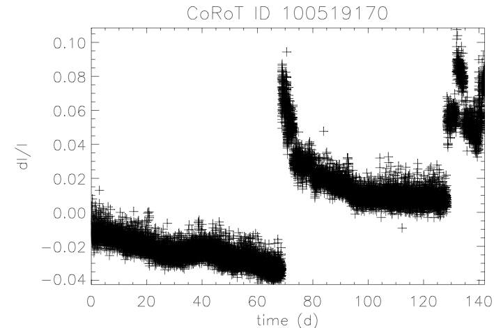
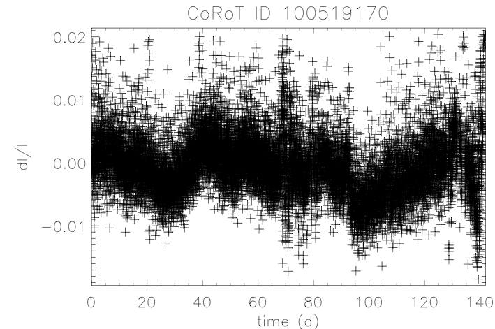
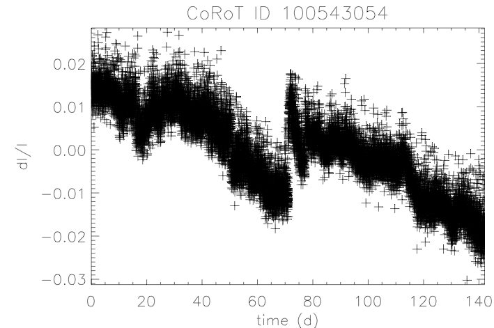
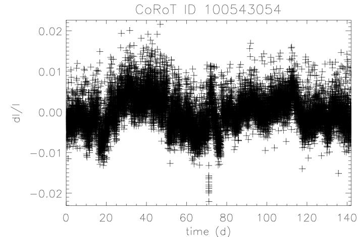
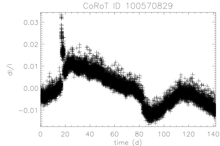
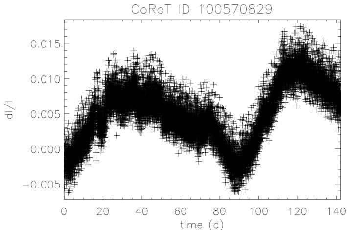
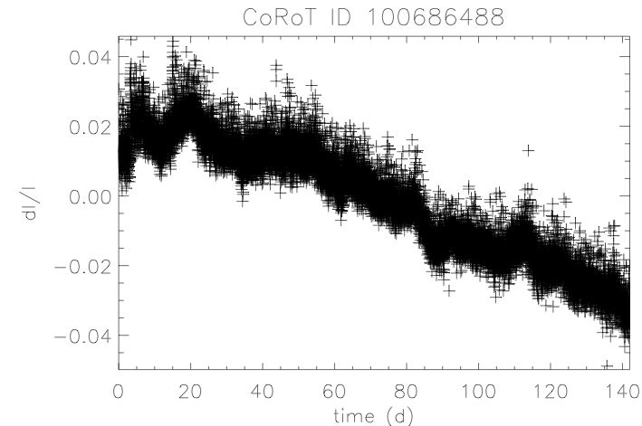
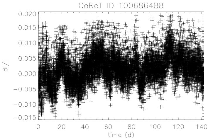
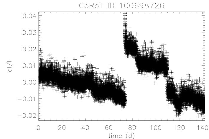
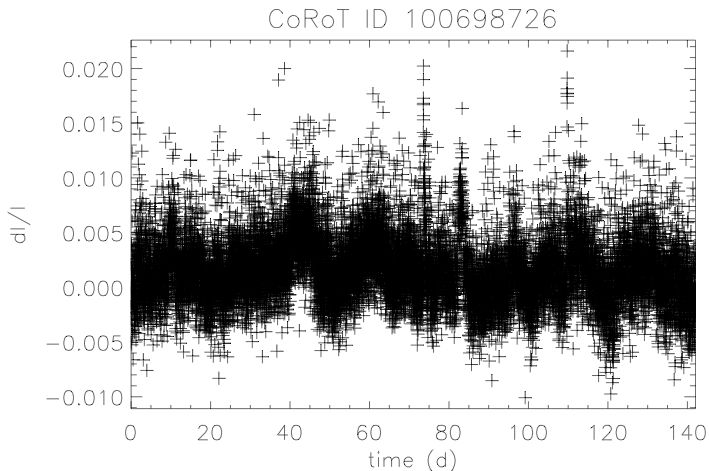
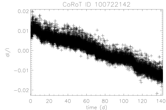
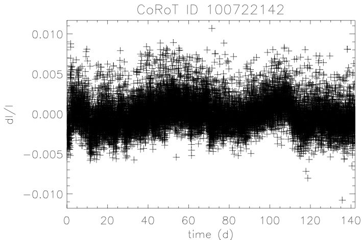
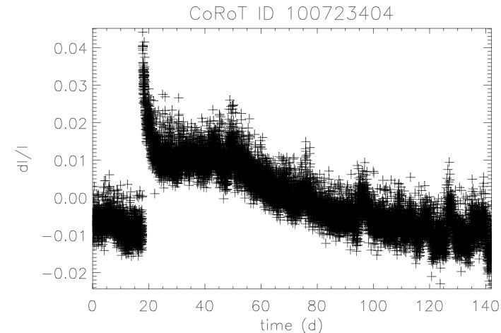
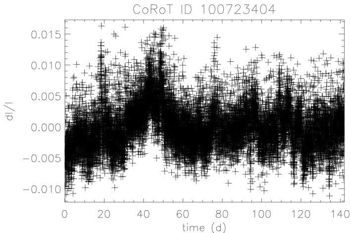
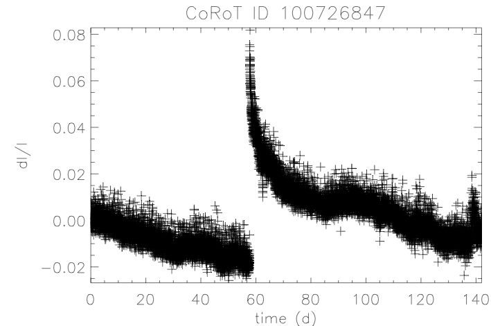
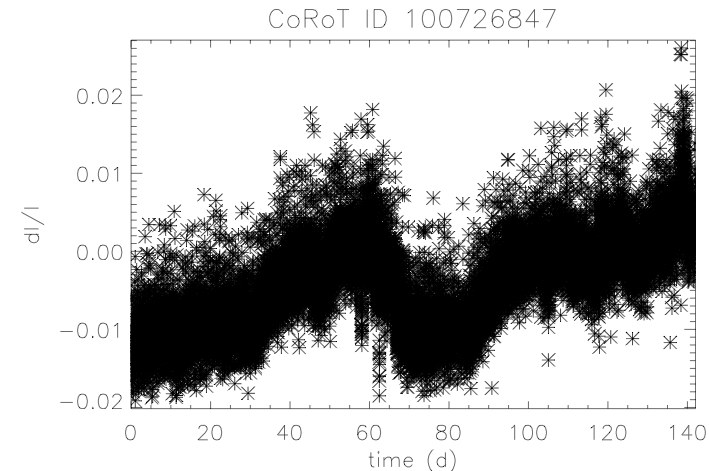
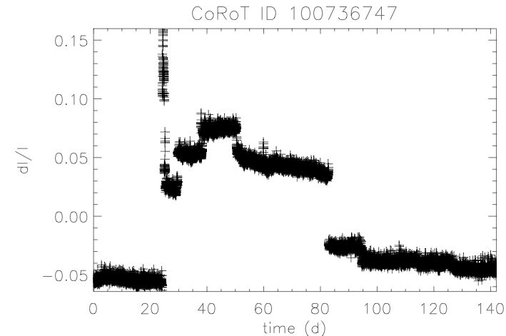
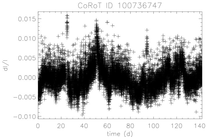
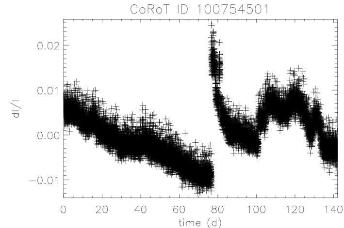
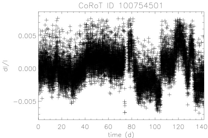
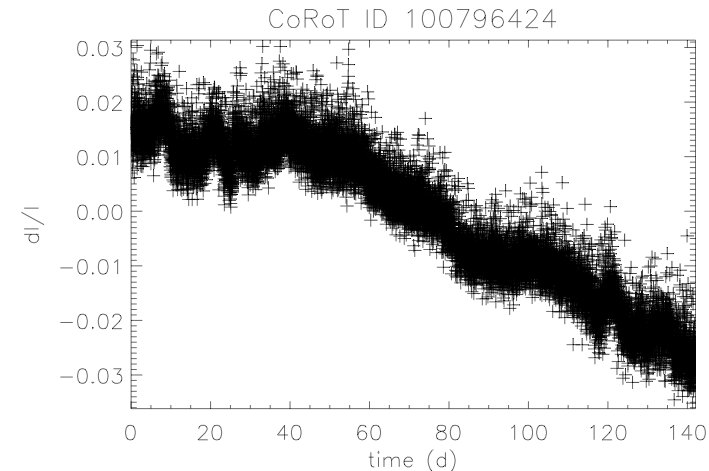
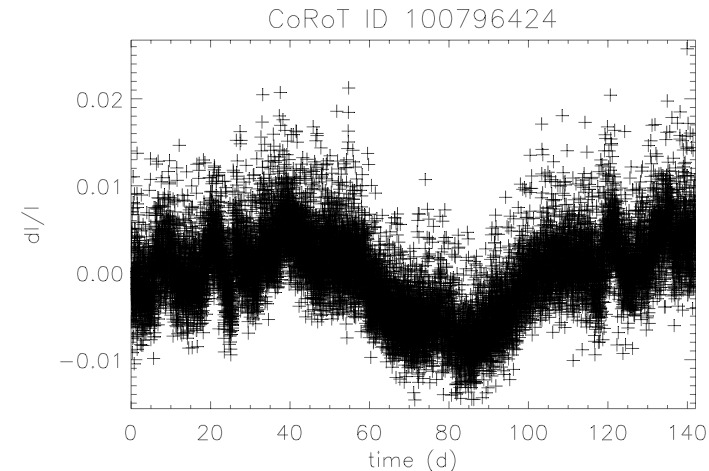
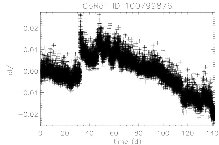
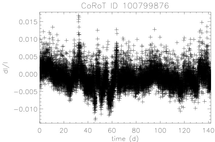
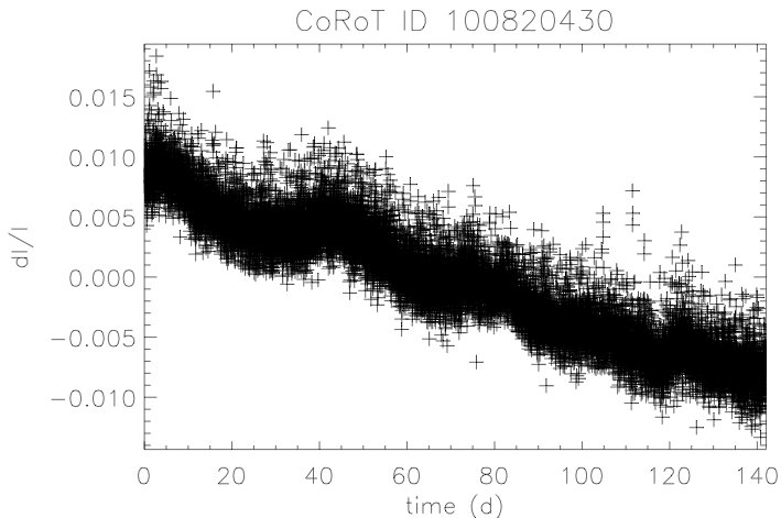
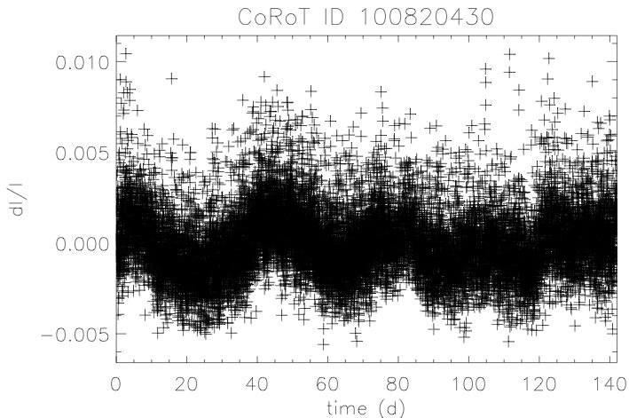
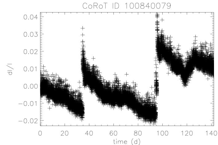
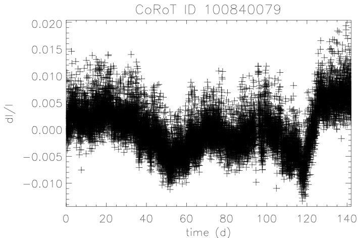
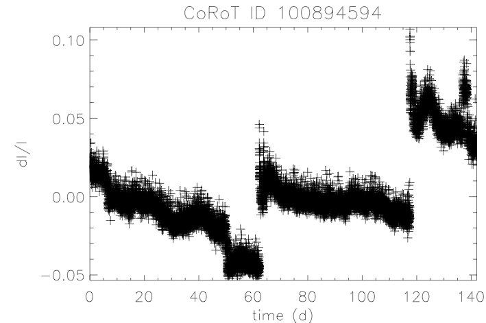
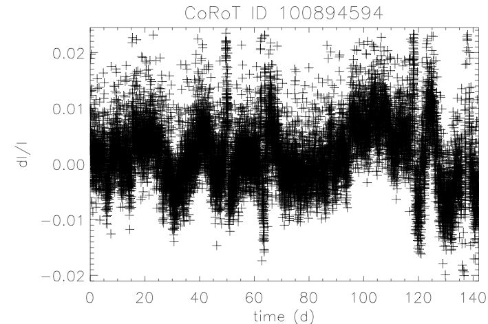
Figure 5: Plot of selected light curves before and after the removal of the discontinuities and/or long-term trends.

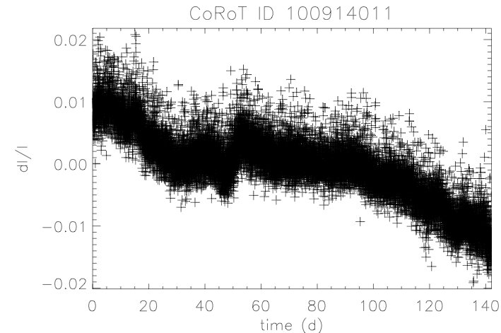
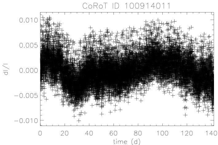
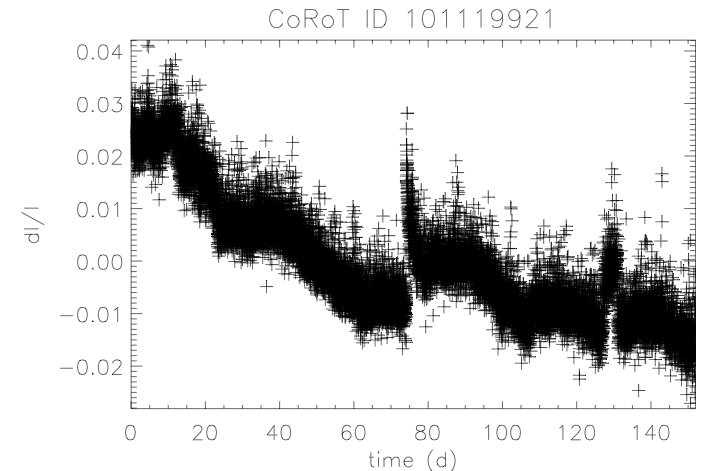
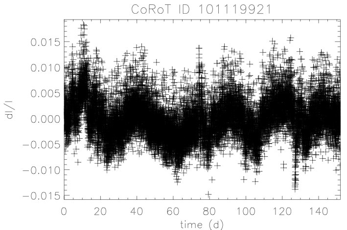
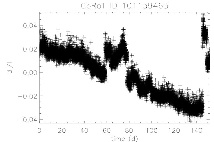
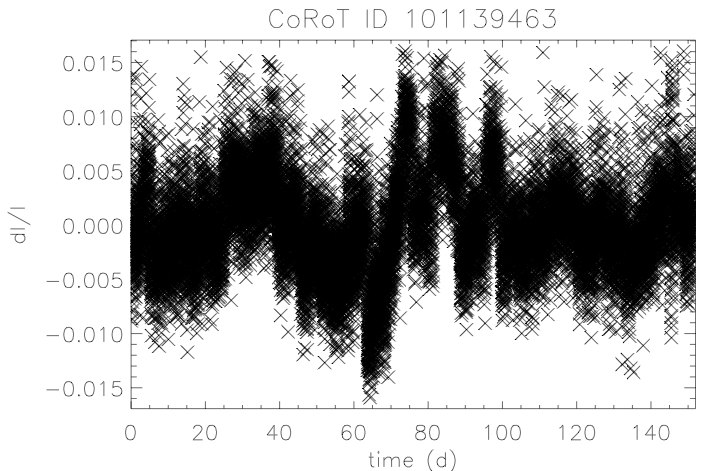
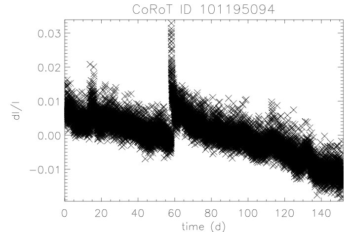
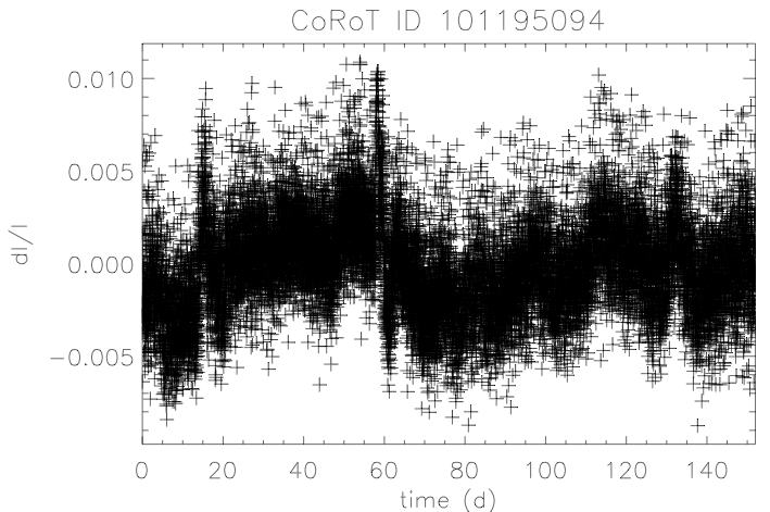
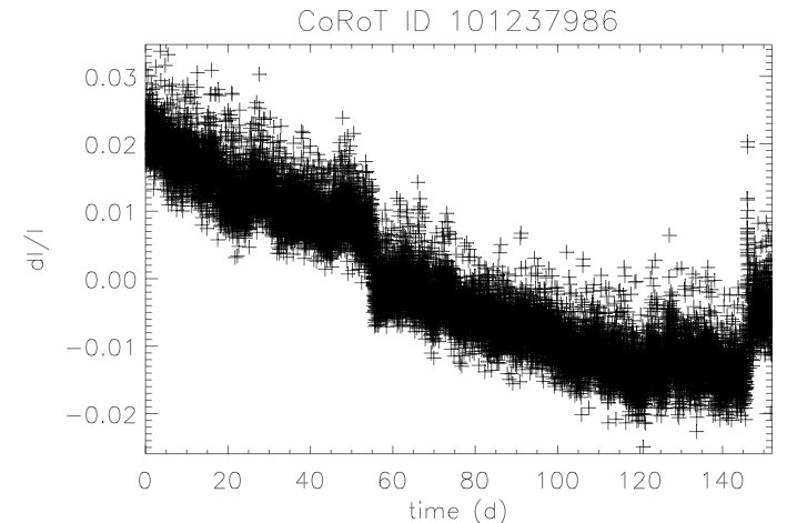
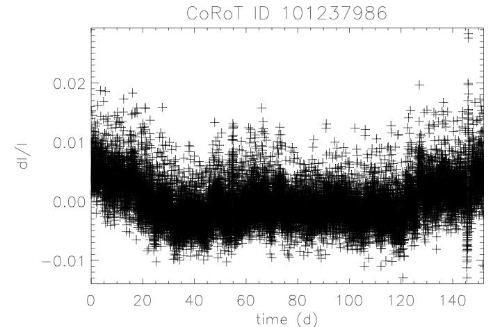
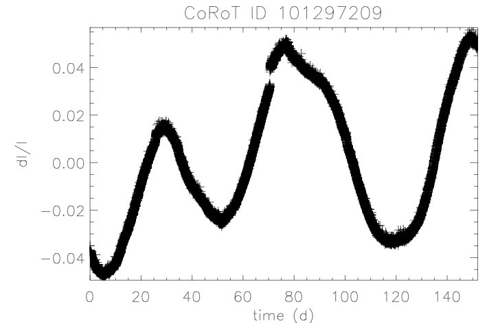
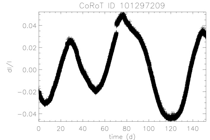
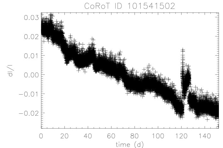
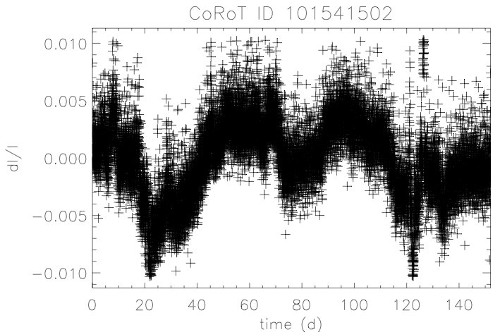
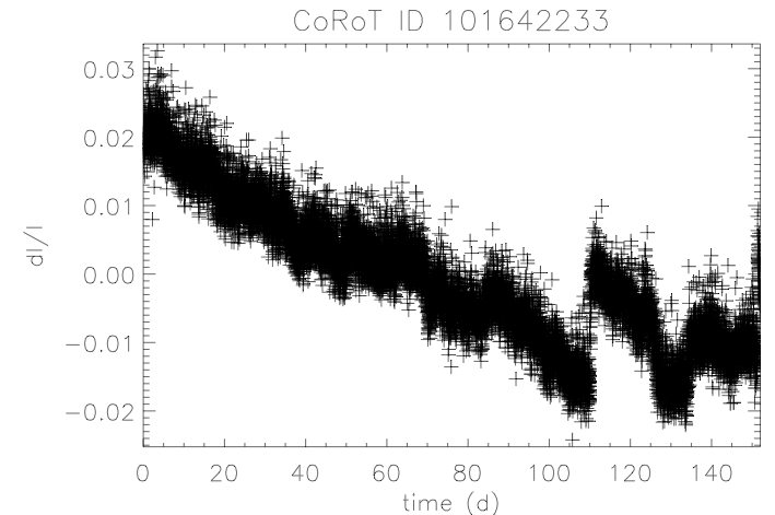
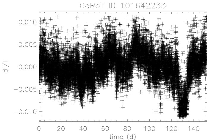
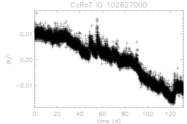
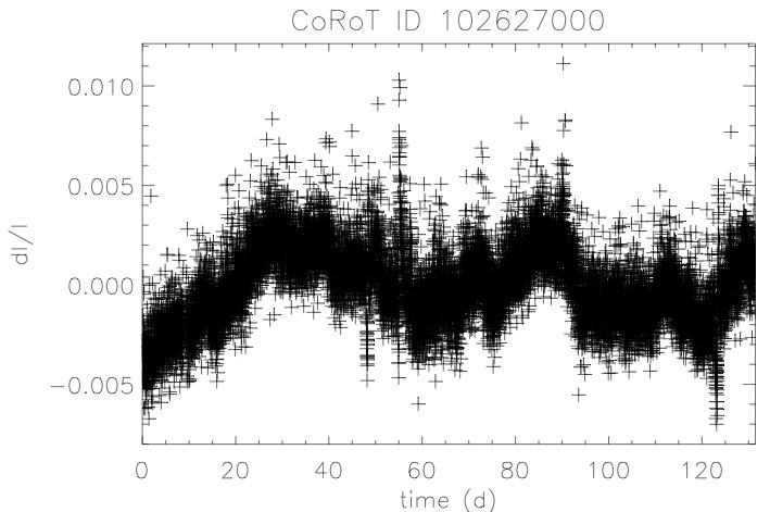
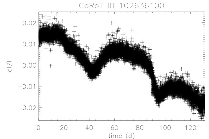
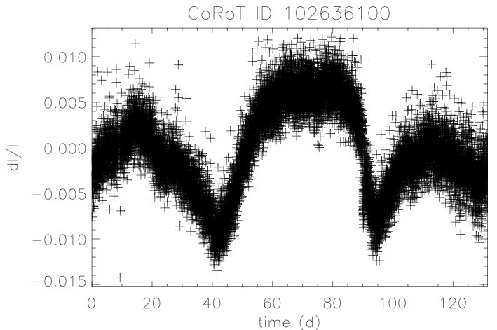
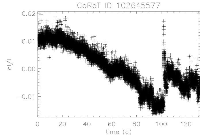
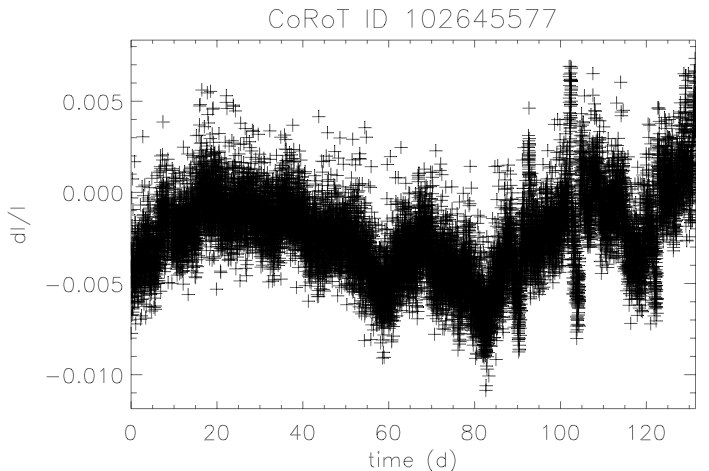
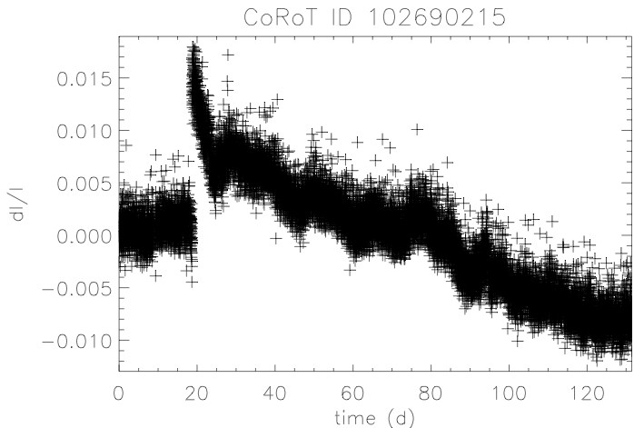
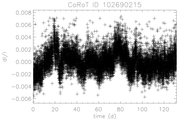
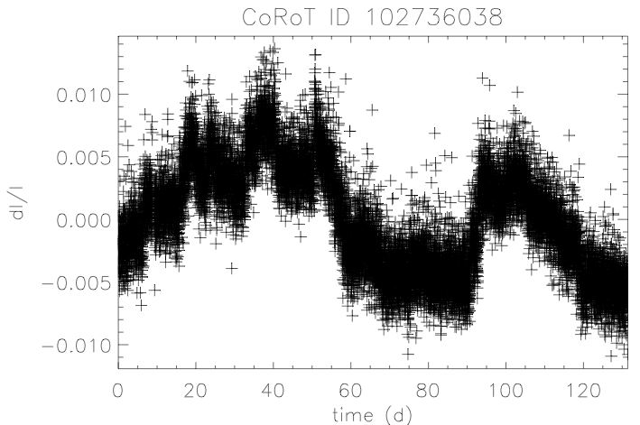
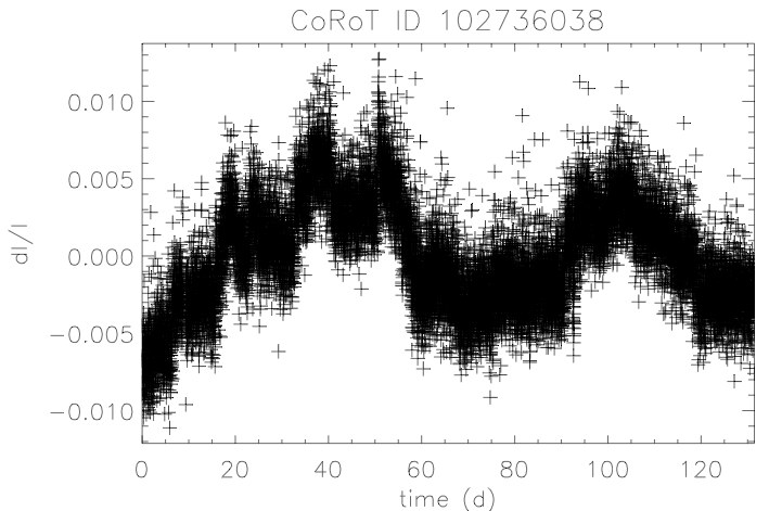
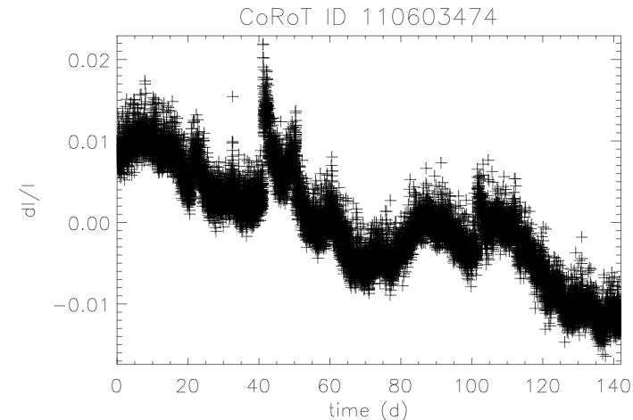
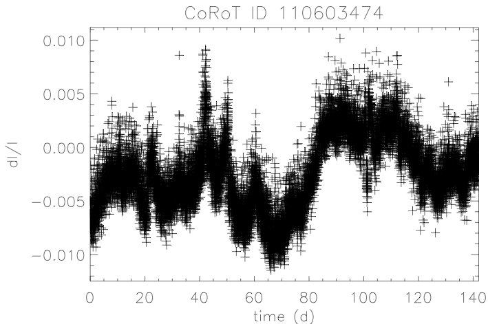
Figure 6: Plot of selected light curves before and after the removal of the discontinuities and/or long-term trends.