A Model of Market Limit Orders By Stochastic PDE’s,
Parameter Estimation, and Investment Optimization

Abstract

In this paper we introduce a completely continuous and time-variate model of the evolution of market limit orders based on the existence, uniqueness, and regularity of the solutions to a type of stochastic partial differential equations obtained in [6]. In contrary to several models proposed and researched in literature, this model provides complete continuity in both time and price inherited from the stochastic PDE, and thus is particularly suitable for the cases where transactions happen in an extremely fast pace, such as those delivered by high frequency traders (HFT’s).

We first elaborate the precise definition of the model with its associated parameters, and show its existence and uniqueness from the related mathematical results given a fixed set of parameters. Then we statistically derive parameter estimation schemes of the model using maximum likelihood and least mean-square-errors estimation methods under certain criteria such as AIC to accommodate to variant number of parameters . Finally as a typical economics and finance use case of the model we settle the investment optimization problem in both static and dynamic sense by analysing the stochastic (Itô) evolution of the utility function of an investor or trader who takes the model and its parameters as exogenous. Two theorems are proved which provide criteria for determining the best (limit) price and time point to make the transaction.

1 Introduction

In literature there have been researches on the modeling of market limit orders and their execution such as [4] and [5], most of which are based on discrete settings, for instance, models based on Poisson processes and/or queuing theory. However, because of rapid technological evolution which brings about ultra-fast microprocessors and hardware, trading behaviors and patterns involved with a large amount of limit order creation, transaction, and cancellation within a short period of time, such as high frequency trading (HFT), have become quite popular and tend to have a heavy impact on the mechanisms of price discovery and formulation. Consequently, a continuous and dynamic model of the evolution of limit orders in a particular market and their dynamics is proposed, which is described by a type of stochastic partial differential equations, Stefan equations, with a number of model parameters to be estimated given a real dataset.

Figure 1: An Illustration of Moving Boundary PDE’s

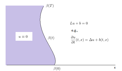
Such type of equations of $u(t,x)$ describes the behavior of a system that consists of two phases, as illustrated in Figure 1, where $\beta(t)$ is a moving boundary which is part of the solution and must be solved simultaneously with $u(t,x)$. As can be seen in Figure 1, in the region to the left of the moving boundary (namely, the set $\{(t,x)\in[0,\infty)\times\mathbb{R}:x\leq\beta(t)\}$) $u$ is constantly set to $0$; on the right side of the boundary (the set $\{(t,x)\in[0,\infty)\times\mathbb{R}:x>\beta(t)\}$) $u$ is described by a PDE of the general form $Lu+b=0$ where $L$ is a predefined second-order differential operator.

For a moving boundary PDE problem, in addition to the regular boundary condition such as the Dirichlet condition $u(t,\beta(t))=0$, there is always an extra boundary condition that describes the dynamics at the moving boundary, for instance, the Stefan boundary condition

$$\frac{\partial u}{\partial x}(t,\beta(t)+)=\rho\dot{\beta}(t).$$ (1)

The type of moving boundary PDE’s we shall use in modeling of market limit order evolution is the Stefan problems, where $L$ is a heat or parabolic operator (for instance, $L:=-\partial/\partial t+\partial^{2}/\partial x^{2}$) with the Stefan boundary condition. Such type of problems has a variety of applications. For instance, in physics, they model the phenomena such as ice melting with the Stefan condition describing the heat balance at the interface (the moving boundary, see [2]); in finance they model the valuation of American options with the PDE derived from the Black-Scholes formula and the moving boundary describing the early exercise price boundary (see Lemma 7.8, Chapter 2, [3]). As it turns out in this paper such equations are also perfectly suitable for modeling the dynamics of high frequency limit order transactions and their evolution, providing statistical parameter estimation methods, and formulating and solving the investment optimization problem based on a typical utility function. Note that [6] provides the mathematical foundation and develops essential techniques that enable us to justify the existence and uniqueness of such type of equations, while obtaining its essential regularities.

In Section 2 we model the evolution of limit orders in a particular market by Stefan equations according to the following facts, and show the existence of such model based on the mathematical results obtained in [6].

1. Limit orders are placed, cancelled, and executed in a manner where jitters tend to be rapidly smoothed out, which is why we have a Laplacian;

2. The change of the mid-price is driven by the intensity of interaction between ask and bid orders around the mid-price;

3. The randomness comes from the constant creation, cancellation, and execution of limit orders; its intensity varies at different (limit) prices, and tends to vanish as the price goes far beyond the mid.

In Section 3 we study the methods to estimate the model parameters based on a given limit order dataset and derive the statistics such as a Maximum-Likelihood Estimator (MLE) and an estimator that minimizes the Mean-Square Errors (MSE), both under AIC (see [1]) since the number of parameters (or dimension) is to be estimated itself. Under certain simplified (or degenerated) circumstances an explicit expression of an MLE estimator is also derived.

In Section 4 we study the investment optimization problem derived from the model, formulate and analyze the static and dynamic properties of the utility function of an investor who takes the model and its parameters as exogenous, which finally enable us to find the optimal limit-price-to-buy (or equivalently, amount-to-buy) of the asset and the corresponding amount of consumption, given a fixed amount of wealth and at a given time. Both static and dynamic analysis are studied to obtain the optimality of the investment via the limit order model, and two theorems are given respectively for those two types of analysis as the criteria to test for optimality from the model dynamics using Itô’s Formula, which also have intuitive interpretations.

2 Modeling

Figure 2: The evolution model of the limit order book

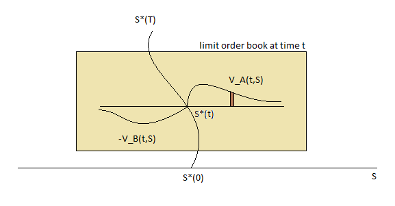
We model the evolution of the limit orders of a particular asset in the market. Suppose we work within the time interval $[0,T]$, and $S$ denotes the natural log of the price so $S\in\mathbb{R}$. At a particular time point $t\in[0,T]$, suppose the volume of the ask (resp. bid) limit orders on the limit order book from $S$ to $S+dS$ is $V_{A}(t,S)dS$ (resp. $V_{B}(t,S)dS$), and suppose the natural log of the mid-price is $S^{*}(t)$. Fix a probability space $(\Omega,\mathcal{F},\mathbb{P})$, We then have the following fairly natural but important model assumptions:

1. all matched orders are executed immediately since all major trading centers today have been computerized, then we have for all $(S,t)$ such that $S>S^{*}(t)$, $V_{B}(S,t)=0$; similarly for all $(S,t)$ such that $S<S^{*}(t)$, $V_{A}(S,t)=0$;

2. since jitters have a tendency to be rapidly smoothed out, $\partial V_{A}/\partial t$ contains a component $\alpha_{A}\Delta V_{A}$ where $\alpha_{A}$ is a positive constant and $\Delta:=\partial^{2}/\partial S^{2}$ is the Laplacian; the same is true for $V_{B}(S,t)$ with $\alpha_{B}$;

3. the change of mid-price is driven by the “strength” of the ask and bid orders placed around the mid-price, which implies we have a Stefan-type condition

   $$\rho\frac{dS^{*}}{dt}(t)=\left[\frac{\partial V_{A}}{\partial S}(t,S^{*}(t)+)+\frac{\partial V_{B}}{\partial S}(t,S^{*}(t)-)\right]$$ (2)

   where $\rho$ is a constant;

4. for $S\geq S^{*}(t)$ the ask orders are placed in a stochastic manner, hence another component of $\partial V_{A}/\partial t$ is $\sigma_{A}(|S-S^{*}(t)|)\frac{\partial^{2}W}{\partial t\partial S}$ where $\sigma_{A}$ is a regular scaling function (defined in Chapter LABEL:Ch:sspw) and $W:\Omega\times[0,T]\times\mathbb{R}\to\mathbb{R}$ is a standard 2-dimensional Brownian sheet; the same is true for $V_{B}$ with $S\leq S^{*}(t)$ and $\sigma_{B}$.

The model is illustrated in Figure 2.

In sum, for a set of given model parameters $u_{0A},u_{0B},\alpha_{A},\alpha_{B},\sigma_{A},\sigma_{B},\rho$, the model has

$$\begin{split}\frac{\partial V_{A}}{\partial t}&=\alpha_{A}\frac{\partial^{2}V_{A}}{\partial S^{2}}+\sigma_{A}(|S-S^{*}(t)|)\frac{\partial^{2}W}{\partial t\partial S},\forall S>S^{*}(t),\\ V_{A}(t,S)&=0,\forall S\leq S^{*}(t),\\ V_{A}(0,S)&=u_{0A}(S),\\ \frac{\partial V_{B}}{\partial t}&=\alpha_{B}\frac{\partial^{2}V_{B}}{\partial S^{2}}+\sigma_{B}(|S-S^{*}(t)|)\frac{\partial^{2}W}{\partial t\partial S},\forall S<S^{*}(t),\\ V_{B}(t,S)&=0,\forall S\geq S^{*}(t),\\ V_{B}(0,S)&=u_{0B}(S),\\ \rho\frac{dS^{*}}{dt}(t)&=\left[\frac{\partial V_{A}}{\partial S}(t,S^{*}(t)+)+\frac{\partial V_{B}}{\partial S}(t,S^{*}(t)-)\right].\end{split}$$ (3)

Theorem 2.1

The solution $V_{A},V_{B},S^{*}$ to model (3) exists and is unique for $0\leq t<\tau$ where $\tau$ is a well-defined stopping time.

• We roughly follow the same procedure to show the existence and uniqueness as in [6]. First we make the following transformation: $\tilde{V}_{A}(t,S):=V_{A}(t,S^{*}(t)+S),\tilde{u}_{0A}(S):=u_{0A}(S^{*}(0)+S),\tilde{V}_{B}(t,S):=V_{B}(t,S^{*}(t)-S),\tilde{u}_{0B}(S):=u_{0B}(S^{*}(0)-S)$. Then the same argument as in Theorem 3.2, [6] shows that there exists unique $\beta_{A},\beta_{B}$ that is the limit of the iteration

  $$\begin{split}\rho\dot{\beta}_{A}^{n}(t)&=\int_{0}^{\infty}\frac{\partial\tilde{p}}{\partial x}(t,0,y)\tilde{u}_{0A}(y)dy+\int_{0}^{t}\int_{0}^{\infty}\frac{\partial\tilde{p}}{\partial x}(t-s,0,y)\sigma_{A}(y)W_{\beta^{n}}(dyds),\\ \rho\dot{\beta}_{B}^{n}(t)&=\int_{0}^{\infty}\frac{\partial\tilde{p}}{\partial x}(t,0,y)\tilde{u}_{0B}(y)dy+\int_{0}^{t}\int_{0}^{\infty}\frac{\partial\tilde{p}}{\partial x}(t-s,0,y)\sigma_{B}(y)W_{\beta^{n}}(dyds),\\ \beta^{n}(t)&=\beta_{A}^{n}(t)-\beta_{B}^{n}(t).\end{split}$$

  Define $S^{*}(t):=\lim_{n}\beta^{n}(t)$ which is also unique. Then using the same argument as in Theorem 3.2, [6], we have that $\tilde{V}_{A}$ and $\tilde{V}_{B}$ exist and are unique. Also, using Kolmogorov’s Continuity Theorem as in Lemma 3.1.1, [6], we have that almost surely,

  $$\begin{split}\rho\dot{\beta}_{A}(t)&=\frac{\partial V_{A}}{\partial S}(t,S^{*}(t)+),\\ \rho\dot{\beta}_{B}(t)&=-\frac{\partial V_{B}}{\partial S}(t,S^{*}(t)-),\end{split}$$

  where $0\leq t<\tau:=\lim_{L\to\infty}\tau^{L}$, and $\tau^{L}:=\inf\{t\geq 0:|\dot{\beta}_{A}(t)|\geq L\textrm{ or }|\dot{\beta}_{B}(t)|\geq L\}$. Therefore the Stefan boundary condition  (2) holds. $\Box$

3 Parameter Estimation

In this section a statistical method based on AIC is developed to estimate the parameters of model (3) given a real dataset of the limit order book and the mid-price of a particular asset within a certain period of time.

Suppose the dataset consists of 3 matrices, two $T\times N$ matrices $D_{A}$, $D_{B}$ for the volumes of the ask and bid orders, and a $T\times 1$ matrix $P$ for the mid-price. The sampling steps for time and price are $\Delta_{T}$ and $\Delta_{N}$, that is, the dataset is from time $0$ to $\Delta_{T}T$, and the $t$-th row of $D_{A}$ stores the volumes of the ask orders from limit price $P[t]$ to $P[t]+\Delta_{N}N$, while the $t$-th row of $D_{B}$ stores the volumes of the bid orders from limit price $P[t]-\Delta_{N}N$ to $P[t]$, where $[\cdot]$ denotes the vector subscription.

Our goal in this section is to develop an algorithm to numerically compute or even find an explicit expression of the statistics served as the appropriate estimators of the model parameters under maximum-likelihood, minimum mean-square errors, and AIC. The method is decomposed into two parts, first parameters $\alpha_{A},\alpha_{B},\sigma_{A},\sigma_{B}$ are estimated using maximum-likelihood approach combined with AIC based on the limit order book data $D_{A}$ and $D_{B}$, and then $u_{0A},u_{0B},\rho$ are estimated using least mean-square-errors combined with AIC based on the whole dataset $D_{A},D_{B},P$.

3.1 AIC/MLE Estimation of $\alpha_{A},\alpha_{B},\sigma_{A},\sigma_{B}$

To estimate $\sigma_{A}$ and $\sigma_{B}$, we further assume that

$$\sigma_{i}(x):=\frac{x^{1.6}}{1+xp_{i}(x)},i=A,B$$

where for $i=A,B$, $p_{i}$ is a polynomial with $\deg p_{i}\geq 1$, so that $\sigma_{i}$ is a regular scaling function, and $\lim_{x\to\infty}\sigma_{i}(x)=0$, because there tends to be very little randomness as the limit price goes far beyond the mid-price. Then the goal is to estimate $\alpha_{A},\alpha_{B}$ and the degrees of $p_{A},p_{B}$ and their coefficients. Since the number of parameters $4+\deg p_{A}+\deg p_{B}$ is also to be estimated, an AIC-based approach is used.

Suppose $i=A,B$, and $p_{i}(x)=\sum_{j=0}^{d_{i}}p_{ij}x^{j}$ with $d_{i}\geq 1$. To estimate $\alpha_{i},p_{i0},\ldots,p_{id_{i}}$, we use a finite-difference Euler approximation scheme similar in Section 4, [6]. For each integer $n$, define the difference operator $\nabla:\mathbb{R}^{n}\to\mathbb{R}^{n-1}$ by

$$\nabla\left((a_{1},\ldots,a_{n})^{T}\right)=\left(a_{2}-a_{1},\ldots,a_{n}-a_{n-1}\right)^{T}.$$

Denote $\left(\nabla a\right)[i]$ by $\nabla a_{i}$. For a matrix with row label $R$ and column label $C$ denote $\nabla_{R}$ as the difference operator on column vectors and $\nabla_{C}$ as that on row vectors. Then for each $i=A,B,t=1,\ldots,T-1,S=1,\ldots,N-2$,

$$\frac{\nabla_{t}D_{i}[t,S]}{\Delta_{T}\Delta_{N}}=\alpha_{i}\frac{\nabla_{S}^{2}D_{i}[t,S]}{\Delta_{N}^{3}}+\sigma_{i}(S\Delta_{N})\frac{\xi_{t,S}}{\Delta_{T}\Delta_{N}}$$

where

$$\xi_{t,S}:=W\left(\left[\Delta_{T}t,\Delta_{T}(t+1)\right]\times\left[S^{*}(\Delta_{T}t)+\Delta_{N}S,S^{*}(\Delta_{T}t)+\Delta_{N}(S+1)\right]\right)$$

are independent identically distributed Gaussian random variables with mean $0$ and variance $\Delta_{T}\Delta_{N}$. Fix $d_{i}=\deg p_{i}$, then the log likelihood function $\ell_{i}(\alpha_{i},p_{i0},\ldots,p_{id_{i}})$ satisfies

$$-2\ell_{i}(\alpha_{i},p_{i0},\ldots,p_{id_{i}})=\sum_{t=1}^{T-1}\sum_{S=1}^{N-2}\left\{\left[\nabla_{t}D_{i}[t,S]-\alpha_{i}\left(\frac{\Delta_{T}}{\Delta_{N}^{2}}\right)\nabla_{S}^{2}D_{i}[t,S]\right]\frac{1+\sum_{j=0}^{d_{i}}p_{ij}S^{j+1}\Delta_{N}^{j+1}}{S^{1.6}\Delta_{N}^{1.6}}\right\}^{2}.$$ (4)

When $d_{i}$ is fixed, the first order condition is a cubic formula of the variables, which shall be solved using numerical methods. If the model can be degenerated so that $\alpha_{i}=\alpha_{0i}$ is a known constant, then we can indeed solve for optimal $\hat{p}_{i0},\ldots,\hat{p}_{id_{i}}$:

$$\textbf{p}_{i}=-\textbf{A}_{i}^{-1}\textbf{b}_{i},$$

where $\textbf{p}_{i}=(\hat{p}_{i0},\ldots,\hat{p}_{id_{i}})^{T}$, $\textbf{A}_{i}$ is a $(d_{i}+1)$-square matrix with its $(m,n)$ element being

$$\sum_{t=1}^{T-1}\sum_{S=1}^{N-2}\left\{\left[\nabla_{t}D_{i}[t,S]-\alpha_{0i}\left(\frac{\Delta_{T}}{\Delta_{N}^{2}}\right)\nabla_{S}^{2}D_{i}[t,S]\right]S^{m+n-3.2}\Delta_{N}^{m+n}\right\}^{2},$$

and $\textbf{b}_{i}$ is a $(d_{i}+1)\times 1$ matrix with its $m$-th element being

$$\sum_{t=1}^{T-1}\sum_{S=1}^{N-2}\left\{\left[\nabla_{t}D_{i}[t,S]-\alpha_{0i}\left(\frac{\Delta_{T}}{\Delta_{N}^{2}}\right)\nabla_{S}^{2}D_{i}[t,S]\right]S^{2m-3.2}\Delta_{N}^{2m}\right\}^{2}.$$

Therefore, under AIC (see [1]), the set of optimal estimators $\hat{\alpha}_{i},\hat{d}_{i},\hat{p}_{i0},\ldots,\hat{p}_{id_{i}}$ minimizes

$$\textrm{AIC}_{i}:=2d_{i}-2\ell_{i}(\alpha_{i},p_{i0},\ldots,p_{id_{i}}).$$ (5)

The algorithm to minimize $\textrm{AIC}_{i}$:

1. $m:=-\infty,\hat{d}_{i}:=0$;

2. For $d_{i}\in\{1,\ldots,10\}$:

   1. Numerically solve the first order condition of (4) for optimal $\hat{\alpha}_{i},\hat{p}_{i0},\ldots,\hat{p}_{id_{i}}$;

   2. Calculate $a:=$AIC($d_{i}$) based on (5);

   3. If $m>a$ then $m:=a,\hat{d}_{i}:=d_{i}$;

3. The final $\hat{d}_{i}$ is optimal within $\{1,\ldots,10\}$ with AIC $m$.

3.2 AIC/Least-MSE Estimation of $u_{0A},u_{0B},\rho$

We continue to assume $i=A,B$. Similarly we need further assumptions about the initial condition $u_{0i}$. Assume

$$u_{0i}(x)=xq_{i}(x)\exp(-\gamma_{i}x)$$

where $q_{i}$ is a polynomial and $\gamma_{i}>0$ is a parameter, so that $u_{0i}$ has exponential decay at infinity. Then $c_{i}:=\deg q_{i}$ and its coefficients $q_{i0},\ldots,q_{ic_{i}}$ are also a model parameter that needs to be determined under AIC. Now, if we take the expectation conditional on $S^{*}$ on both sides of the evolution equation of $V_{i}$, we get

$$\mathbb{E}[V_{i}(t,S)|S^{*}]=\int_{0}^{\infty}p_{-}(t,S,y)u_{0i}(y)dy+\int_{0}^{t}S^{*}(s)\int_{0}^{\infty}q(t-s,S,y)\mathbb{E}[V_{i}(s,y)|S^{*}]dyds.$$

This implies that $\mathbb{E}[V_{i}|S^{*}]$ satisfies a deterministic Stefan-type PDE, which means that although we are generally unable to find an explicit expression of the solution, we can find a sufficiently accurate numerical solution. For a given dataset $D_{A},D_{B},P$, the goal in this part is thus to develop an algorithm to minimize the mean-square errors against $\mathbb{E}[V_{i}|S^{*}]$ and the mid-price function (moving boundary) determined by it under AIC.

Given a set of parameters $c_{A},c_{B},q_{A0},\ldots,q_{Ac_{A}},q_{B0},\ldots,q_{Bc_{B}},\gamma_{A},\gamma_{B},\rho$, denote the solution to the deterministic Stefan-type PDE (i.e., when $W\equiv 0$) by $\bar{V}_{A}$ and $\bar{V}_{B}$, which can be obtained numerically. Then the variances (errors) come from two parts: those from the evolution of the limit order book, and those from the evolution of the mid-price. Let $\theta_{0}$ be a predefined constant which is the weight of importance of how well mid-price fits against how well the limit order book fits. Namely, we shall minimize the weighted MSE

$$\textrm{MSE}:=\textrm{MSE}_{1}+\theta_{0}\textrm{MSE}_{2}$$

where

$$\textrm{MSE}_{1}:=\frac{1}{2TN}\sum_{i\in\{A,B\}}\sum_{t=1}^{T}\sum_{S=1}^{N}\left[D_{i}(t,S)-\bar{V}_{i}(\Delta_{T}t,\Delta_{N}S)\right]^{2},$$

and

$$\textrm{MSE}_{2}:=\frac{1}{T}\sum_{t=1}^{T}\left[\rho P(t)-\frac{\bar{V}_{A}(\Delta_{T}t,S)+\bar{V}_{B}(\Delta_{T}t,S)}{\Delta_{T}}\right]^{2}.$$

Finally, similar to the AIC approach in the previous part, the goal is to minimize

$$c_{A}+c_{B}+\textrm{MSE},$$

which can be done by traversing all possible values of the model parameters, numerically finding $\bar{V}_{A}$ and $\bar{V}_{B}$, computing the corresponding MSE’s, and finally finding the recorded optimal parameters. Note that unlike in previous part, because of the nonlinearity of $\bar{V}_{A}$ and $\bar{V}_{B}$, it is difficult to find a direct way to (numerically) solve for optimal coefficients for $q_{i}$, as opposed to $p_{i}$.

4 Investment Optimization

Using the model combined with a set of optimal parameters adjusted for a given dataset, an investor can optimize his or her allocation of the amount of investment in the asset against consumption within a given amount of wealth. To analyze the investment behavior under our model, we assume the investor can only buy a single asset by making limit order transactions, that is, fulfilling ask orders placed by other sellers. This scenario is typical when an investor is avert to the volatility of price changes in market order transactions, or there lacks sufficient liquidity of the asset but the investor still has a strong motivation to make purchases.

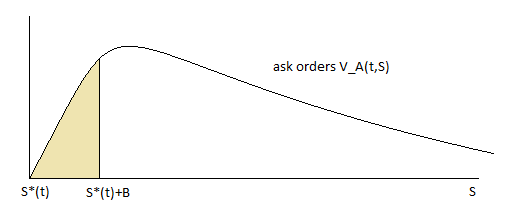
Let $U:\mathbb{R}_{+}^{3}\to\mathbb{R}$ be the utility function of the investor, which is monotone increasing and concave down on the second and third parameters. Specifically, $U(t,L_{t},C_{t})$ denotes the amount of happiness the investor obtains at time $t$ if having the amount of asset $L_{t}$ and consumption $C_{t}$. Since the investor would choose to pay the lowest possible price to buy an amount of asset, the amount of asset $L_{t}$ and the total cost to buy such amount is completely determined by the highest limit price $S^{*}(t)+B$ the investor is willing to pay, which is illustrated in Figure 3.

Figure 3: Investment Optimization via Limit Orders

Taking the model (and its parameters) as exogenous, and assuming the time $t$ wealth is $W_{t}$, we then have the following optimization problem at time $t$ (where the subscription $t$ in the expectation denotes it is conditional to all information up to time $t$):

$$\max_{B\geq 0}\mathbb{E}_{t}\left[U\left(t,L_{t}(B),C_{t}\right)\right]$$

where

$$L_{t}(B)=\int_{S^{*}(t)}^{S^{*}(t)+B}V_{A}(t,S)dS$$

subject to the budget constraint

$$W_{t}=C_{t}+\int_{S^{*}(t)}^{S^{*}(t)+B}SV_{A}(t,S)dS.$$

When $t$ is fixed, the optimization of $U$ with respect to the choice of $B$ is done through a static analysis; if we consider the full model, that is, both $t$ and $B$ vary, we come up with a dynamic analysis.

4.1 Static Analysis

Let time $t$ be fixed. Denote the partial derivatives of $U$ by $U_{t},U_{L},U_{C}$. Then we compute

$$\begin{split}\frac{\partial U}{\partial B}(t,L_{t}(B),C_{t})&=U_{L}(t,L_{t}(B),C_{t})V_{A}(t,S^{*}(t)+B)\\ &\quad\quad-U_{C}(t,L_{t}(B),C_{t})(S^{*}(t)+B)V_{A}(t,S^{*}(t)+B).\end{split}$$

Therefore the optimal $B=B^{*}$ satisfies the first order condition

$$S^{*}(t)+B^{*}=\frac{U_{L}(t,L_{t}(B^{*}),C_{t})}{U_{C}(t,L_{t}(B^{*}),C_{t})}.$$

This means

Theorem 4.1

In static optimization where the time $t$ is fixed, the optimal highest limit price to buy the asset is equal to the ratio of the marginal utility of amount of asset to that of consumption.

• As above. $\Box$

Note that $S^{*}(t)+B^{*}$ can be seen as the highest amount of money the investor is willing to pay to substitute $1$ unit of asset with the same amount of consumption.

4.2 Dynamic Analysis

Now consider that $t$ also varies, and we are interested in $\mathbb{E}_{t}[dU]$ from $t$ to $t+dt$. Indeed, if we have $\mathbb{E}_{t}[dU(t,L_{t}(B^{*}),C_{t})]>0$, then even if $B=B^{*}$ reaches its static optimality, the investor would still wait for an amount of time to maximize the utility.

First we consider the evolution of $L_{t}(B)$. Fixing $B$ and plugging in $dV_{A}$, we have formally

$$\begin{split}dL_{t}(B)&=\alpha_{A}\left[\frac{\partial V_{A}}{\partial S}(t,S^{*}(t)+B)-\frac{\partial V_{A}}{\partial S}(t,S^{*}(t))\right]dt\\ &\quad\quad+\int_{S^{*}(t)}^{S^{*}(t)+B}\sigma(S-S^{*}(t))W(dSdt)\\ &\quad\quad+\left[\int_{0}^{t}\int_{S^{*}(t)}^{S^{*}(t)+B}\sigma(S-S^{*}(t))W(dSdt)\right]\dot{S}^{*}(t)dt.\end{split}$$

Similarly,

$$\begin{split}dC_{t}&=\alpha_{A}\left[V_{A}(t,S^{*}(t)+B)-(S^{*}(t)+B)\frac{\partial V_{A}}{\partial S}(t,S^{*}(t)+B)+S^{*}(t)\frac{\partial V_{A}}{\partial S}(t,S^{*}(t))\right]dt\\ &\quad\quad+\int_{S^{*}(t)}^{S^{*}(t)+B}S\sigma(S-S^{*}(t))W(dSdt)\\ &\quad\quad+\left[\int_{0}^{t}\int_{S^{*}(t)}^{S^{*}(t)+B}S\sigma(S-S^{*}(t))W(dSdt)\right]\dot{S}^{*}(t)dt.\end{split}$$

Then by Itô’s formula, and noting that $S^{*}(t)$ is part of the information at $t$, we get

$$\begin{split}\mathbb{E}_{t}[dU]&=U_{t}dt+U_{L}\alpha_{A}\left[\frac{\partial V_{A}}{\partial S}(t,S^{*}(t)+B)-\frac{\partial V_{A}}{\partial S}(t,S^{*}(t))\right]dt+\frac{1}{2}U_{LL}\int_{0}^{B}\sigma^{2}(S)dSdt\\ &\quad\quad+U_{C}\alpha_{A}\left[V_{A}(t,S^{*}(t)+B)-(S^{*}(t)+B)\frac{\partial V_{A}}{\partial S}(t,S^{*}(t)+B)+S^{*}(t)\frac{\partial V_{A}}{\partial S}(t,S^{*}(t))\right]dt\\ &\quad\quad+\frac{1}{2}U_{CC}\int_{0}^{B}(S^{*}(t)+S)^{2}\sigma^{2}(S)dSdt.\end{split}$$

Since for a fixed $t$ we are only interested at $B^{*}$ in Theorem 4.1, and $S^{*}+B^{*}=U_{L}/U_{C}$, we have

$$\begin{split}\mathbb{E}_{t}\left[\frac{dU}{dt}(t,L_{t}(B^{*}),C_{t})\right]&=U_{t}+U_{C}\alpha_{A}\left[V_{A}(t,S^{*}(t)+B^{*})-B^{*}\frac{\partial V_{A}}{\partial S}(t,S^{*}(t))\right]\\ &\quad\quad+\frac{1}{2}U_{LL}\int_{0}^{B^{*}}\sigma^{2}(S)dS+\frac{1}{2}U_{CC}\int_{0}^{B^{*}}(S^{*}(t)+S)^{2}\sigma^{2}(S)dS.\end{split}$$ (6)

If we denote the absolute risk aversions of the investor with respect to the amount of asset and the consumption by

$$\begin{split}r_{L}&:=-\frac{U_{LL}}{U_{L}},\\ r_{C}&:=-\frac{U_{CC}}{U_{C}},\end{split}$$

then (6) is equivalent to

$$\begin{split}\mathbb{E}_{t}\left[\frac{dU}{dt}(t,L_{t}(B^{*}),C_{t})\right]&=U_{t}+U_{C}\left\{\alpha_{A}\left[V_{A}(t,S^{*}(t)+B^{*})-B^{*}\frac{\partial V_{A}}{\partial S}(t,S^{*}(t))\right]\right.\\ &\quad\quad\left.-\frac{1}{2}r_{L}(S^{*}+B^{*})\int_{0}^{B^{*}}\sigma^{2}(S)dS-\frac{1}{2}r_{C}\int_{0}^{B^{*}}(S^{*}+S)^{2}\sigma^{2}(S)dS\right\}.\end{split}$$ (7)

The investor would then use the dataset $D_{A}$ to compute $\mathbb{E}_{t}\left[\frac{dU}{dt}\right]$ and see the expected change of $U$ from $t$ to $t+dt$ at $B^{*}$. Specifically, we have the following observations from Equation (6) or (7):

1. the larger the quantity

   $$V_{A}(t,S^{*}(t)+B^{*})-B^{*}\frac{\partial V_{A}}{\partial S}(t,S^{*}(t))$$

   is, the more possible it is for $U$ to increase;

2. the greater absolute risk aversions $r_{L}$ and $r_{C}$ the investor has, the more possible it is for $U$ to decrease;

3. the larger $B^{*}$ is, the more risk $U$ is exposed to for a decrease, since both $\int_{0}^{B^{*}}\sigma^{2}(S)dS$ and $\int_{0}^{B^{*}}(S^{*}+S)^{2}\sigma^{2}(S)dS$ are increasing functions of $B^{*}$.

Also, if we make two natural assumptions about $U$,

1. the utility function is discounted in time, that is, $U_{t}<0$,

2. the investor is risk avert or risk neutral, that is, $U_{LL}\leq 0,U_{CC}\leq 0$,

then we have

Theorem 4.2

Suppose $B^{*}$ is the statically optimal choice at time $t$ as in Theorem 4.1. If

$$V_{A}(t,S^{*}(t)+B^{*})\leq B^{*}\frac{\partial V_{A}}{\partial S}(t,S^{*}(t)),$$ (8)

then

$$\mathbb{E}_{t}\left[\frac{dU}{dt}(t,L_{t}(B^{*}),C_{t})\right]\leq 0.$$

• As above. $\Box$

Figure 4: An Illustration of Theorem 4.2

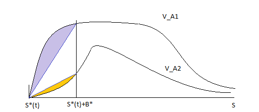
Note that (8) in Theorem 4.2 has an intuitive illustration in Figure 4. The quantity $V_{A}(t,S^{*}(t)+B^{*})/B^{*}$ is the slope of the colored lines between the mid-price point $(S^{*}(t),0)$ and the optimal point $(S^{*}+B^{*},V_{A}(t,S^{*}+B^{*}))$.

1. If it is less than the boundary derivative $\partial V_{A}(t,S^{*}(t))/\partial S$ as shown in curve $V_{A1}$, then the utility at next instant $t+dt$ is expected to drop, as the volume of ask orders at lower limit prices between $S^{*}$ and $S^{*}+B^{*}$ tends to fall, so it is best to make the purchase at $t$ rather than wait.

2. On the other hand, as shown in curve $V_{A2}$, the volume at lower prices tends to rise, and it might be wise to wait for a future time to make the purchase. In this case the investor needs to evaluate other factors such as time discount $U_{t}$ and risk premium terms as well.

5 Summary

In this chapter we summarize the main results obtained in the previous sections. Throughout this chapter we fix a probability space $(\Omega,\mathcal{F},\mathbb{P})$, and suppose $W:\Omega\times\mathbb{R}\times\mathbb{R}\to\mathbb{R}$ is a standard 2-dimensional Brownian sheet.

5.1 Modeling

For a set of given model parameters $u_{0A},u_{0B},\alpha_{A},\alpha_{B},\sigma_{A},\sigma_{B},\rho$, the model

$$\begin{split}\frac{\partial V_{A}}{\partial t}&=\alpha_{A}\frac{\partial^{2}V_{A}}{\partial S^{2}}+\sigma_{A}(|S-S^{*}(t)|)\frac{\partial^{2}W}{\partial t\partial S},\forall S>S^{*}(t),\\ V_{A}(t,S)&=0,\forall S\leq S^{*}(t),\\ V_{A}(0,S)&=u_{0A}(S),\\ \frac{\partial V_{B}}{\partial t}&=\alpha_{B}\frac{\partial^{2}V_{B}}{\partial S^{2}}+\sigma_{B}(|S-S^{*}(t)|)\frac{\partial^{2}W}{\partial t\partial S},\forall S<S^{*}(t),\\ V_{B}(t,S)&=0,\forall S\geq S^{*}(t),\\ V_{B}(0,S)&=u_{0B}(S),\\ \rho\frac{dS^{*}}{dt}(t)&=\left[\frac{\partial V_{A}}{\partial S}(t,S^{*}(t)+)+\frac{\partial V_{B}}{\partial S}(t,S^{*}(t)-)\right]\end{split}$$ (9)

exists and is unique.

5.2 Parameter Estimation

Suppose $P,D_{A},D_{B}$ is a given limit order dataset. For $i=A,B$, suppose

$$\sigma_{i}(x):=\frac{x^{1.6}}{1+xp_{i}(x)},i=A,B$$

where $p_{i}=\sum_{j=0}^{d_{i}}p_{ij}x^{j}$ is a polynomial with $\deg p_{i}\geq 1$. Then the first step is to minimize for $i=A,B$,

$$\begin{split}\textrm{AIC}_{i}&:=2d_{i}-2\ell_{i}(\alpha_{i},p_{i0},\ldots,p_{id_{i}})\\ &=\sum_{t=1}^{T-1}\sum_{S=1}^{N-2}\left\{\left[\nabla_{t}D_{i}[t,S]-\alpha_{i}\left(\frac{\Delta_{T}}{\Delta_{N}^{2}}\right)\nabla_{S}^{2}D_{i}[t,S]\right]\frac{1+\sum_{j=0}^{d_{i}}p_{ij}S^{j+1}\Delta_{N}^{j+1}}{S^{1.6}\Delta_{N}^{1.6}}\right\}^{2}.\end{split}$$ (10)

Suppose also

$$u_{0i}(x)=xq_{i}(x)\exp(-\gamma_{i}x)$$

where $q_{i}=\sum_{j=0}^{c_{i}}q_{ij}x^{j}$ is a polynomial and $\gamma_{i}>0$ is a parameter. Then the second step is for a predefined weight $\theta_{0}$ to minimize

$$c_{A}+c_{B}+\textrm{MSE}_{1}+\theta_{0}\textrm{MSE}_{2}$$

where

$$\begin{split}\textrm{MSE}_{1}&:=\frac{1}{2TN}\sum_{i\in\{A,B\}}\sum_{t=1}^{T}\sum_{S=1}^{N}\left[D_{i}(t,S)-\bar{V}_{i}(\Delta_{T}t,\Delta_{N}S)\right]^{2},\\ \textrm{MSE}_{2}&:=\frac{1}{T}\sum_{t=1}^{T}\left[\rho P(t)-\frac{\bar{V}_{A}(\Delta_{T}t,S)+\bar{V}_{B}(\Delta_{T}t,S)}{\Delta_{T}}\right]^{2},\end{split}$$

and $\bar{V}_{i}(t,x)$ is the numerical solution by setting $W\equiv 0$.

5.3 Optimization

Suppose $B^{*}(t)$ is the statically optimal price at time $t$ with respect to the utility function $U$ and wealth $W_{t}$. Then

$$S^{*}(t)+B^{*}(t)=\frac{U_{L}(t,L_{t}(B^{*}(t)),C_{t})}{U_{C}(t,L_{t}(B^{*}(t)),C_{t})}.$$

In other words, the optimal highest limit price to buy the asset is equal to the ratio of the marginal utility of amount of asset to that of consumption.

Also, let $r_{L},r_{C}$ be the absolute risk aversions with respect to $L,C$, then we have

$$\begin{split}\mathbb{E}_{t}\left[\frac{dU}{dt}(t,L_{t}(B^{*}),C_{t})\right]&=U_{t}+U_{C}\left\{\alpha_{A}\left[V_{A}(t,S^{*}(t)+B^{*})-B^{*}\frac{\partial V_{A}}{\partial S}(t,S^{*}(t))\right]\right.\\ &\quad\quad\left.-\frac{1}{2}r_{L}(S^{*}+B^{*})\int_{0}^{B^{*}}\sigma^{2}(S)dS-\frac{1}{2}r_{C}\int_{0}^{B^{*}}(S^{*}+S)^{2}\sigma^{2}(S)dS\right\}.\end{split}$$ (11)

In particular, if

$$\frac{V_{A}(t,S^{*}(t)+B^{*})}{B^{*}}\leq\frac{\partial V_{A}}{\partial S}(t,S^{*}(t)),$$ (12)

then

$$\mathbb{E}_{t}\left[\frac{dU}{dt}(t,L_{t}(B^{*}),C_{t})\right]\leq 0.$$

References

- [1] Hirotsugu Akaike. A new look at the statistical model identification. IEEE Transactions on Automatic Control, 1974.
- [2] Avner Friedman. Partial differential equations of parabolic type. Prentice-Hall Inc., 1964.
- [3] Ioannis Karatzas and Steven E. Shreve. Methods of Mathematical Finance. Springer-Verlag, 1998.
- [4] Andrew W. Lo, Craig A. MacKinlay, and June Zhang. Econometric models of limit-order executives. Journal of Financial Economics, 2002.
- [5] Ioanid Roşu. A dynamic model of the limit order book. Review of Financial Studies, 2009.
- [6] Zhi Zheng and Richard B. Sowers. Stochastic stefan problems driven by standard brownian sheets. arXiv/Math/Probability, 2012.