What planetary nebulae tell us about helium and the CNO elements in Galactic bulge stars

Abstract

Thermally pulsing asymptotic giant branch (TP-AGB) models of bulge stars are calculated using a synthetic model. The goal is to infer typical progenitor masses and compositions by reproducing the typical chemical composition and central star masses of planetary nebulae (PNe) in the Galactic bulge. The AGB tip luminosity and the observation that the observed lack of bright carbon stars in the bulge are matched by the models.

Five sets of galactic bulge PNe were analyzed to find typical abundances and central star of planetary nebulae (CSPN) masses. These global parameters were matched by the AGB models. These sets are shown to be consistent with the most massive CSPN having the largest abundances of helium and heavy elements. The CSPN masses of the most helium rich (He/H$\ga$0.130 or $Y\ga 0.34$) PNe are estimated to be between 0.58 and 0.62$\,{\rm M}_{\sun}$. The oxygen abundance in form $\log{\rm(O/H)}+12$ of these highest mass CSPN is estimated to be $\approx$8.85.

TP-AGB models with ZAMS masses between 1.2 and 1.8$\,{\rm M}_{\sun}$ with $Y_{\rm ZAMS}\approx 0.31-0.33$ and $Z_{\rm ZAMS}\approx 0.19-0.22$ fit the typical global parameters, mass, and abundances of the highest mass CSPN. The inferred ZAMS helium abundance of the most metal enriched stars implies $dY/dZ\sim 4$ for the Galactic bulge. These models produce no bright carbon stars in agreement with observations of the bulge. These models produce an AGB tip luminosity for the bulge in agreement with the observations. These models suggest the youngest main sequence stars in the Galactic bulge have enhanced helium abundance ($Y\approx 0.32$) on the main sequence and their ages are between 2 and 4 Gyrs.

The chemical evolution of nitrogen in the Galactic bulge inferred from the models is consistent with the cosmic evolution inferred from HII regions and unevolved stars. The inferred ZAMS N/O ratio ($\log{\rm N/O}\approx-0.35$) of bulge PNe with the largest CSPN masses are shown to be above the solar ratio. The inferred ZAMS N/O ratios of the entire range of PNe metallicities is consistent with both primary and secondary production of nitrogen contributing to the chemical evolution of nitrogen in the Galactic bulge.

The inferred ZAMS value of C/O is less than 1. This indicates the mass of the PNe progenitors are low enough (M$\la 1.8\,{\rm M}_{\sun}$) to not produce carbon stars via the third dredge-up.

Accepted 2012 October 15. Received 2012 October 12; in original form 2012 June 18

1 Introduction

Galactic bulge planetary nebulae (GB-PNe) are an important set of stars for the study of the stellar and chemical evolution of stars. These important stars give information about the ages of different populations of stars. The central star planetary nebulae (CSPN) mass should be related to the zero-age main sequence (ZAMS) mass of the progenitors. PNe allow direct measurements of the abundances of important atoms which are difficult to directly measure in other stars such as helium, neon and argon.

An important unsettled question about the bulge is whether it contains both old and young populations of stars or just old populations? There are two contradictory lines of evidence about this question. Photometric studies of the luminosity of the galactic bulge main sequence turn-off (MSTO) indicate it is faint (kr02; zo03; br10; cl11). This suggests most star formation in the bulge ended around $\sim 10\,{\rm Gyr}$ ago. This view has been challenged by the work of ben10; ben11 using spectroscopy of stars during microlensing events. They found the position of Galactic bulge stars on the $\log{g}-\log{T_{eff}}$ plane near the MSTO and on the subgiant branch. In the same study the abundances of several elements were measured allowing a determination of chemistry. This is important since the positions of isochrones vary by [Fe/H] and [$\alpha$/Fe]. To fit these stars with the correct metallicity isochrones, much younger isochrones then those used in the photometric studies were needed for a proper fit. The youngest Galactic bulge stars in ben11 have inferred ages of $\sim 3.0\,{\rm Gyr}$. This suggests, in contradiction of the photometry studies, there exists a significant population of younger stars in the bulge.

ng12 suggested a way to reconcile these two disparate interpretations. They suggested that there is a population which is older than that suggested by ben10; ben11 but younger than 10$\,{\rm Gyr}$ suggested by photometric studies. They argue such a population reconciles these two disparate observations with essentially two old populations; one with enhanced values of $Y$ and one with normal values of $Y$. They argue that both the photometric and spectroscopic studies use of non-helium enhanced isochrones give the wrong inferred ages and masses of bulge stars. Their argument is that if helium enhanced isochrones are used for comparison to the MSTO in the photometric studies, a younger age would be indicated. If helium enhanced isochrones are used to compare to the results from the spectroscopic studies of (ben10; ben11) older ages would be indicated. This would bring these contradictory results at least nearer to agreement.

na11 also found indirect evidence that there are stars with enhanced $Y$ in the bulge. They attributed the anomalous Galactic bulge red giant branch bump to a population of stars with an enhanced value of $Y$ ($Y\sim 0.35$).

An enhanced value of $Y$ in ZAMS stars is not unprecedented. Globular clusters in the Milky Way and the Magellanic Clouds show evidence of the existence of multiple populations with distinct values of $Y$. The extensive spectroscopic evidence is reviewed in gratreview and the photometric evidence of multiple main-sequences, sub-giant branches, red giant branches and horizontal branches in the same globular cluster is reviewed in sqrev09. In many (and possibly all) globular clusters there are at least two chemically distinct populations. The older population (primary) consists of stars with scaled-solar abundances and a helium abundance which can be determined by linearly interpolating in $Z$ from the primordial helium abundace, $Y_{0}$, to the solar helium abundance, $Y_{\sun}$. The slightly younger population (secondary) consists of stars with an enhanced abundance of helium ($\Delta Y$) which can be very modest ($\approx 0.01$) or large ($\approx 0.12$). The enhancement of helium is defined as the increase of the helium fraction over what would be determined from the equation:

$$Y=Y_{0}+(dY/dZ)Z$$ (1)

where $Z$ is the metallicity.

There are several available abundance studies of Galactic bulge PNe (hereinafter GB-PNe) which measure the abundance of helium (rat92; rat97; cui00; liu01; esc04; ex04; wl07; chi09). All of these studies show some GB-PNe have an elevated He/H (Defined here as He/H$>$0.120). In each of these studies the highest level of He/H for each lies between 0.135 and 0.22. For a PN in the disc or other region where there is active star formation an elevated He/H would be interpreted as the result of helium enhanced material being mixed up from the interior to the surface of the star. The amount of this enhancement is greatest for intermediate-mass stars (defined as M$\ga 3.5\,{\rm M}_{\sun}$). The surface helium abundance of intermediate-mass stars is increased by the action of the second dredge-up (SDU), the third dredge-up (TDU) and the action of hot-bottom burning (HBB). HBB occurs at the base of the convective envelope of a thermally pulsing asymptotic giant branch (TP-AGB) star when the temperature at the base becomes high enough for the CN cycle to operate. HBB is limited to intermediate-mass stars ($\ga 3.5\,{\rm M}_{\sun}$) and converts C to N while producing some He. The SDU occurs when the star enters the early-AGB (E-AGB) and material which experienced complete hydrogen buring is mixed up to the surface. A result of SDU is to raise the surface abundance of helium. Theoretically to get a SDU a star needs a ZAMS mass of $\ga 4.0{\rm M}_{\sun}$ (bs99). The TDU occurs near the end of a helium shell flash when during the TP-AGB the convective envelope penetrates into a region where partial helium burning has taken place. However, to significantly enhance the abundance of helium and nitrogen requires an intermediate-mass star (M$\ga 3.5\,{\rm M}_{\sun}$. The lifetime of such a star is short ($\la 0.5\,{\rm Gyr}$).

If intermediate-mass stars are the progenitors of the high helium bulge PNe then they would come from a very young population. This hypothetical very young population would be younger than the results of ben10; ben11 would indicate. Since a significant number of the bulge PNe have high helium abundances generally associated with intermediate-mass stars, but there are not significant numbers of intermediate-mass stars in the bulge, there must be an alternative explanation of the observed high helium abundances. The observed range of GB-PNe He/H is 0.09-0.20. Assuming the progenitor has near solar abundances, $Y\approx 0.27$ and $Z\approx 0.017$ (vsp12), to produce a helium abundance this high requires a star of mass of $\ga 4\,{\rm M}_{\sun}$ (gj93; mar99) with a lifetime of $\la 0.4\,{\rm Gyr}$. Main sequence stars of this mass are not observed in the bulge. It seems unlikely there are stars of this mass in the bulge since it would mean there would be AGB stars brighter than seen in the bulge. If intermediate-mass stars exist in the bulge, it would mean main sequence stars with masses between 2 and 4$\,{\rm M}_{\sun}$ would also exist in the bulge. These 2-4$\,{\rm M}_{\sun}$ would produce bright carbon stars. This contradicts the observation that the C-stars in the bulge are faint. Faint carbon stars are interpreted as carbon-enriched low-mass stars resulting from a binary mass-transfer event.

The alternative is that the progenitors of these PNe are older low-mass stars which formed with high helium abundance. The PNe abundances would then reflect the initial abundances with minor modifications due to the first dredge up (FDU) only. The FDU effects stars of all mass and occurs when the star enters the red giant branch (RGB). During the FDU the abundances of He and N are slightly increased at the expense of a decrease in the C abundance. bu12 (hereinafter Paper I) presented a similar model to explain the two PNe in globular clusters (JaFu 1 and JaFu 2) both of which have elevated helium abundances but are clearly from an old, low-mass population. Paper I showed the global parameters of both the PNe (helium abundance, oxygen abundance, mass of central star) and the parameters inferred from the host cluster (metallicity and progenitor mass) can be matched by low-mass, helium enhanced models.

The goal of this paper is to test if the GB-PNe can be explained with a low-mass model and to use their observed global parameters to infer the ZAMS mass and the ZAMS $Y$ value. In Section 2 the TP-AGB models are discussed. In Section 3 the abundances and CSPN masses of GB-PNe as well as other relevant observations are reviewed with the goal of determining appropriate global averages to compare to the models. In Section 4 the models are presented and compared to the observations. In Section LABEL:sec:diss the implications are discussed. In Section LABEL:sec:con conclusions and suggestions for further work are presented.

2 Models

To model the evolutionary behavior of the stars the model described in Paper I is used. Briefly, this model calculates the structure of the envelope during the interpulse period of the TP-AGB by geting the luminosity from a core-mass luminosity relation. The effects of pre-TP-AGB evolution are modeled using fits to published models. Most of the relevant details of this model are explained in bu97, bue97, and gbm. In paper I the most significant update to the model was an updated rule for treating the mass-loss during the red giant branch (RGB) and early-AGB (E-AGB) phases. This is a significant model input, especially for low-mass ZAMS stars which can lose an appreciable fraction of their mass during the RGB and E-AGB. In paper I, particular attention was paid to the effect of an enhanced helium abundances on mass-loss during these stages. The mass-loss in these stages was found by integrating the mass-loss rate formula over the Padova tracks. There is an important point to note, in paper I the calculation of pre-TP-AGB mass-loss model, as noted by the referee of that paper, the evolution of the star and the mass-loss rates are not coupled. The amount of mass-loss found with these equations are quite reasonable but the reader should be aware of it. For the masses of the stars modeled here (M$=1.1-1.8\,{\rm M}_{\sun}$) any errors in the pre-TP-AGB mass-loss will not have a large effect on the subsequent evolution of the star.

2.1 Elemental abundances

The solar abundance set used in this paper is from asp05. This set was chosen because the oxygen abundance ($\epsilon{\rm(O)}=8.66$) is similar to that found in Galactic HII regions such as the Orion Nebula. A typical value of oxygen for the Orion Nebula is slightly higher, e.g. $\epsilon{\rm(O)}=8.74$ (e.g. sd11).

Abundances for stars are usually published as in terms of $[{\rm Fe/H}]$. At sub-solar $[{\rm Fe/H}]$ the $\alpha$ elements are known to be enhanced. At $[{\rm Fe/H}]\la-1.0$ the $\alpha$ elements are enhanced relative to iron by a constant factor. The level of the $\alpha$ plateau is expressed as

$$[\alpha/{\rm Fe}]=k_{1}$$ (2)

where $k_{1}$ is an adjustable parameter. In this model this parameter which will be set to approximately +0.4. At a value of $[{\rm Fe/H}]\approx-1$ the value of $[\alpha/{\rm Fe}]$ begins to decrease linearly and reaches a value of zero at $[{\rm Fe/H}]=0$. The position of this knee in the distribution is given by

$$[{\rm Fe/H}]_{\rm knee}=k_{2}.$$ (3)

The mass fraction of helium $Y$ is computing an intermediate scaled solar value, $Y_{ss}$ is computed by

$$Y_{ss}=Y_{0}+\frac{dY}{dZ}Z$$ (4)

where $Y_{0}$ is the primordial helium mass fraction and $\frac{dY}{dZ}$ is the slope of the relationship between $Y$ and $Z$. The mass fraction of helium is then enhanced by an adjustable factor $\Delta Y$. The equation is given by

$$Y=Y_{ss}+\Delta Y.$$ (5)

Since the element nitrogen shows considerable variation the abundance of nitrogen can be enhanced by a factor $\Delta{\rm N}$. When nitrogen is enhanced the value of $Z$ is enhanced by the same amount. The mass fraction of hydrogen is calculated from

$$X=1-Y-Z.$$ (6)

2.2 Red giant mass-loss

The mass-loss which occurs on the red giant branch (RGB) is very important for low-mass stars, which in some extreme cases may prevent the star from even reaching the TP-AGB. Most of the pre-TP-AGB mass-loss occurs during the RGB. The standard method to determine the amount of mass-loss is to use Reimers’ Law (rei) given by

$$\dot{M}=\eta\frac{LR}{M}$$ (7)

where L, R and M are the stellar luminosity, radius and mass, respectively in solar units. However, in this paper the pre-TP-AGB mass-loss was calculated using an updated and modified version of the Reimers formula of (sch) given by

$$\dot{M}=\eta\frac{LR}{M}(\frac{T_{\rm eff}}{4000{\rm K}})^{3.5}(1+\frac{g_{\sun}}{4300g_{\star}})$$ (8)

where $T_{\rm eff}$ is the effective stellar temperature, $g_{\star}$ is the surface gravity of the star in cgs units. Values of 27400${\rm cms^{-2}}$ for $g_{\sun}$ and $8.0\times 10^{-14}$ for $\eta$ were adopted, which are the values recommended by (sch). This new mass-loss rule appears to give better results for horizontal branch masses then the Reimer’s rate (sch).

This mass-loss law was applied to the variable $Y$ stellar evolution tracks from the Padova stellar evolutionary library (http://pleadi.pd.astro.it) described in detail in berta and bertb. To determine the red giant mass-loss the mass-loss rate was integrated from the beginning of the red giant branch (encoded in the Padova files as brgbs) up to the tip of the red giant branch (encoded as trgb) using the trapezoidal rule. The amount of mass-loss between time steps in the models is given by

$$\Delta M_{i}=\frac{1}{2}(\dot{m}_{i+1}+\dot{m}_{i})(t_{i+1}-t_{i})$$ (9)

where $t_{i}$ and $t_{i+1}$ are the model times and $\dot{m}_{i+1}$ and $\dot{m}_{i}$ are the mass-loss rates at the corresponding times. The total mass-loss is determined by summing all of the $\Delta M_{i}$s.

Paper I gives the mass-losses for the RGB and E-AGB for the Padova models with metallicities of solar ($Z=0.017$) and lower. Since bulge metallicities are higher (and potentially super-solar) the mass-losses for the higher than solar metallicities are presented in this paper.

The mass-losses on the RGB as a function of the ZAMS mass for all available values of $Y$ for $Z=0.04$ and $Z=0.07$ are shown in Figure 1 by the points. In all panels it is evident the amount of mass-loss decreases as $Y$ increases. This occurs because stars with higher values of $Y$ means the RGB star will have smaller radii and higher surface gravity due to the lower opacity in the outer layers. These factors lower the mass-loss rates and the total mass-loss.

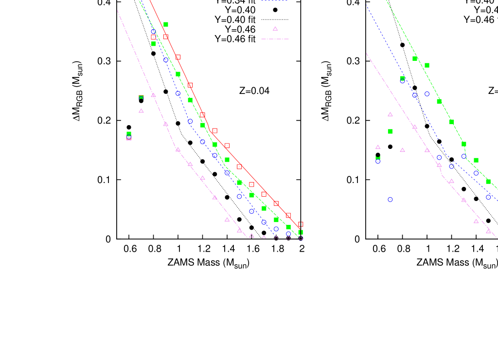
Figure 1: Each panel in the figure shows the calculated mass-loss on the red giant branch for the $Z$=0.04 and 0.07 for the available values of $Y$. The red open squares, green filled squares, blue open circles, black closed circles and violet triangles are the calculated mass-losses for $Y$=0.26, 0.30, 0.34, 0.40 and 0.46, respectively. The red solid, green dashed, blue short dashed, black dotted and violet long-dashed dotted lines are the fits for the $Y$=0.26, 0.30, 0.34, 0.40, and 0.46 mass-losses, respectively.

The RGB mass-loss was fit using two linear fits for higher and lower ZAMS masses. The transition point between the fits was determined by visually estimating the mass where the slope appears to change. This mass is typically found around a ZAMS mass of 0.8-0.9 M${}_{\sun}$. The higher mass fit was terminated where the high mass line crosses the horizontal axis. This termination point was estimated visually. For masses larger than $\approx 2.0\,{\rm M}_{\sun}$ the mass-loss is 0. The equations of the linear fits for low and high masses are given by $\Delta{\rm M}_{\rm RGB,low}$ and $\Delta{\rm M}_{\rm RGB,high}$. To make the fits work the fitting was done by excluding the ${\rm M}\leq 0.9\,{\rm M}_{\sun}$ models. These can be safely excluded since the mass-loss for these very low-mass stars eliminates their envelope before the tip of the RGB is reached and such models will not be considered in this paper. Visual inspection indicates the fits are in good agreement to the mass-loss calculations.

The equations for $\Delta{\rm M}_{\rm RGB,low}$ and $\Delta{\rm M}_{\rm RGB,high}$ are given by

$$\Delta{\rm M}_{\rm RGB,low}=a_{11}M+a_{10}$$ (10)

$$\Delta{\rm M}_{\rm RGB,high}=a_{21}M+a_{20}.$$ (11)

The mass-loss is found by calculating the value of both $\Delta{\rm M}$s and finding the maximum value. If the mass-loss is found to be negative then the value of the mass-loss is set to 0. The coefficients of these equations for the different values of $Y$ and $Z$ are shown in Table 1.

Table 1: Red giant mass-loss coefficients

$Z$	$Y$	$a_{11}$	$a_{10}$	$a_{21}$	$a_{20}$
0.040	0.26	-0.442678	0.744023	-0.225394	0.466268
0.040	0.30	-0.638065	0.929548	-0.230933	0.455032
0.040	0.34	-0.522	0.769042	-0.270372	0.489416
0.040	0.40	-0.589165	0.782297	-0.269874	0.454302
0.040	0.46	-0.48654	0.630983	-0.26096	0.410264
0.070	0.30	-0.3836	0.659316	-0.200032	0.399528
0.070	0.34	-0.384918	0.588526	-0.185168	0.356611
0.070	0.40	-0.684775	0.873781	-0.267901	0.447723
0.070	0.46	-0.3217	0.475414	-0.23702	0.373474

A couple of caveats need to be noted. No attempt has been made yet to calibrate this mass-loss, which will be done in a later paper. However, the mass-loss values from these equations appear to be reasonable. For example a $1.0\,{\rm M}_{\sun}$ $Y=0.26$ $Z=0.017$ star would experience 0.28$\,{\rm M}_{\sun}$ of mass-loss on the RGB which is typical of other models. A typical globular cluster turn-off mass of $0.80\,{\rm M}_{\sun}$ with $Y=0.245$ and $Z=0.0008$ gives a RGB mass-loss of 0.22$\,{\rm M}_{\sun}$. This is reasonable since it gives a zero-age horizontal branch mass of approximately 0.58$\,{\rm M}_{\sun}$ which is similar to measured values (e.g. grat10).

It should be noted, as suggested by the referee of paper I, that the method used to find the mass-loss is not consistent with the stellar evolution models. As the star loses mass its surface gravity would decrease causing the star to expand. For the models used this would result in a higher mass-loss rate near the tip of the RGB and a greater amount of mass-loss on the RGB (and the E-AGB) than is calculated here. However, this effect should be relatively small since the deviation will only be really significant at the tip of the RGB. Although the method used here is not strictly consistent the relative differences in mass-loss due to the effect of the ZAMS helium abundances and the ZAMS metallicity should be correct.

It was noted by the referee of this paper that mig12 argued the RGB mass loss inferred by asteroseismology for the old, metal-rich ($Z\approx 0.04$) open cluster NGC6791 is $0.09\pm 0.03$. This is approximately one half of the red giant mass loss as determined from the formulas above. The MSTO mass of NGC6791 is 1.23$\,{\rm M}_{\sun}$. The amount of RGB mass loss predicted for the prescription here is $\sim 0.17\,{\rm M}_{\sun}$. The relatively small difference between the mass loss will make little difference to the subsequent AGB evolution. In the bulge the most massive PN progenitors will have masses between 1.2 and 1.8$\,{\rm M}_{\sun}$ and only a relatively small amount of mass ($\la 0.1\,{\rm M}_{\sun}$) is lost on the RGB and E-AGB. Most of the mass loss occurs on the TP-AGB when the star evolves to the superwind phase. During this phase the mass loss rates are $10^{-5}$ to $10^{-4}{\rm M}_{\sun}{\rm yr}^{-1}$. In models when the star reaches the superwind phase with an additional 0.1$\,{\rm M}_{\sun}{\rm yr}^{-1}$ of envelope mass, it produces a model CSPN with an observationally neglibly different mass. To verify this some models were run with a pre-AGB mass loss with one half of the value from the prescription above and the difference in the CSPN mass is found to be small.

2.3 Mass-loss on the early-AGB

The same procedure to determine the mass-loss on the RGB was applied to the early-AGB (E-AGB) portions of the Padova tracks. An additional condition of starting the mass-loss when the temperature was below 4500K was assumed since this mass-loss law is applicable only to K and M stars.

Figure 2 shows the calculated mass-loss during the E-AGB and the fits to these mass-losses. The mass-loss on the E-AGB is fit using 4 fits in different regions of mass. The lowest mass range (${\rm M}\la 1.5\,{\rm M}_{\sun}$) is fit via a cubic, the next mass range up ($1.5\,{\rm M}_{\sun}\la{\rm M}\la 2.0\,{\rm M}_{\sun}$) is fit using a quadratic fit. The next mass range up ($2.0\,{\rm M}_{\sun}\la{\rm M}\la 4.5\,{\rm M}_{\sun}$) is fit using a linear fit. Finally the highest masses are fit using a constant value of mass-loss. The points of intersection between adjacent fits were visually estimated. This procedure gives a good fit to the model mass-losses.

The equations for the E-AGB mass-loss in the first two mass regions are given by

$$\Delta{\rm M}_{\rm E-AGB}=a_{13}M^{3}+a_{12}M^{2}+a_{11}M+a_{10}$$ (12)

and

$$\Delta{\rm M}_{\rm E-AGB}=a_{22}M^{2}+a_{21}M+a_{20}$$ (13)

where $M$ is the mass of the star on the ZAMS. Only the coefficients of first two regions have been included in Table 2 to save space and since no models of sufficient mass which need the fits for the upper regions are calculated in this paper. The coefficients for lower metallicities are presented in paper I. The E-AGB mass-loss is calculated by finding the intersection of the two regions and then choosing the appropriate region and plugging into the corresponding equation.

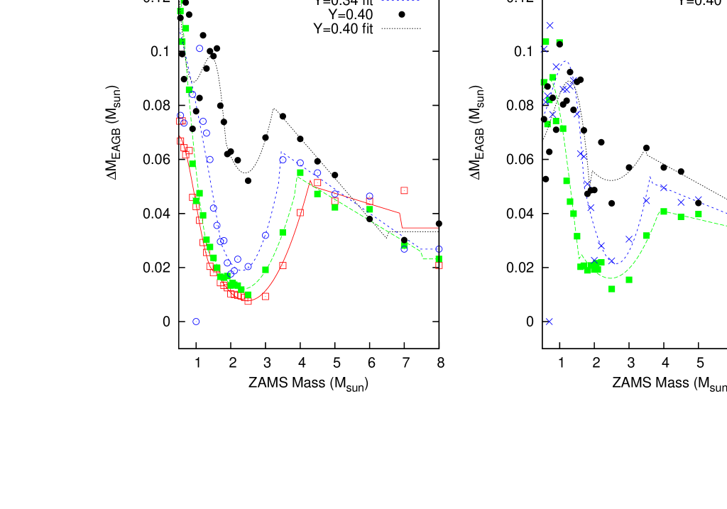
Figure 2: Each panel in the figure shows the calculated mass-loss on the early asymptotic giant branch as a function of ZAMS mass for the $Z=$0.04 and 0.07 models for different available values of $Y$. The symbols and lines have the same meaning as those in Figure 1.

Table 2: Coefficients for fits to early-AGB mass-loss

$Z$	$Y$	$a_{13}$	$a_{12}$	$a_{11}$	$a_{10}$	$a_{22}$	$a_{21}$	$a_{20}$
0.040	0.26	0.0858588	-0.256145	0.182936	0.030799	0.0135521	-0.0670728	0.0906499
0.040	0.3	0.0435809	-0.0520068	-0.144506	0.208967	0.0154136	-0.0720782	0.0962957
0.040	0.4	-0.156291	0.552081	-0.620921	0.314167	0.0361522	-0.174489	0.265491
0.040	0.34	0.00445069	-0.0255256	-0.0266288	0.128011	0.028588	-0.13232	0.171976
0.070	0.3	0.0697326	-0.29361	0.306202	-0.00452271	0.0126149	-0.0622221	0.0927601
0.070	0.4	-0.0565319	0.135358	-0.0691988	0.0744541	0.0122269	-0.0607111	0.127542
0.070	0.34	-0.203047	0.640541	-0.631658	0.273183	0.0337056	-0.177336	0.254678

2.4 Core mass at the first pulse

From the Padova stellar evolution library the core mass at the onset of the first thermal pulse as a function of the ZAMS mass was extracted. The tables with this information are found under the agb files are found at vizier.u-strasbg.fr in the catalog J/A+A/508/355. Figure 3 shows the mass of the carbon-oxygen core as a function of mass for several values of $Y$ and $Z$. An important point to note is that as the initial helium mass fraction increases so does the mass of the core. The core mass is important since it is the most important factor controlling the luminosity of an AGB star. The core mass at the first pulse should also correlate with the resulting CSPN mass.

Figure 3 show the core mass at the first pulse from the Padova models for $Z=$0.04 and 0.07 and $Y=$0.26, 0.30, 0.34 and 0.40 as a function of mass. Each set of models with a given $Y$ and $Z$ have been fit by a double quadratic fit, one at lower masses ($\la 1.5\,{\rm M}_{\sun}$) and one at higher masses. The transition between the two was found between 1.3 and 2.0 ${\rm M}_{\sun}$. The transition between the lower mass and higher masses was determined by visual inspection of where the core mass begins to rise steeply. In all cases the fits to the points and the fit equations are yield core masses which are typically less than 0.02${\rm M}_{\sun}$ different from the calculated points.

The equations of the quadratic fits for low and high masses are given by ${\rm M}_{\rm c0,low}$ and ${\rm M}_{\rm c0,high}$. The equations are

$${\rm M}_{\rm c0,low}=a_{12}M^{2}+a_{11}M+a_{10}$$ (14)

$${\rm M}_{\rm c0,high}=a_{22}M^{2}+a_{21}M+a_{20}$$ (15)

where M is the ZAMS mass. The coefficients for the different values of $Y$ and $Z$ are shown in Table 3. The procedure used is to find the point of intersection between the two fits and then to plug in the relevant mass.

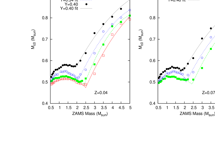
Figure 3: The figure shows the core mass at the onset of the first pulse for the $Z=$0.04 and 0.07 models and the fits to these curves. The symbols have the same meaning as they do in Figure 1.

Table 3: Coefficients for the fits to the first pulse core masses

$Z$	$Y$	$a_{12}$	$a_{11}$	$a_{10}$	$a_{22}$	$a_{21}$	$a_{20}$
0.040	0.26	-0.0325831	0.0910294	0.451145	-0.0202143	0.284259	-0.1105
0.040	0.30	-0.0291444	0.0765474	0.473872	-0.0337214	0.375711	-0.222486
0.040	0.34	-0.0625541	0.16101	0.444288	-0.0211523	0.26243	0.0542981
0.040	0.40	-0.0483516	0.145099	0.470201	-0.015598	0.211713	0.215733
0.070	0.30	-0.0318383	0.0896357	0.45999	-0.0265214	0.314122	-0.118729
0.070	0.34	-0.071077	0.198063	0.410435	-0.0196009	0.246253	0.0692979
0.070	0.40	-0.0601748	0.169262	0.449156	-0.0167222	0.214947	0.195378

The most obvious trend is there is an increase in the core mass as the value of $Y$ increases. This is important since on the AGB a larger core mass leads to a higher luminosity. This is also important since the mass at the first pulse is an important factor in determining the mass of the CSPN. For a constant ZAMS mass a higher ZAMS $Y$ value should lead to a higher CSPN mass.

2.5 Third dredge-up

In synthetic AGB models the standard method to model the TDU effect is to use a dredge-up parameter $\lambda$ where

$$\lambda=\frac{\Delta M_{\rm dredge}}{\Delta M_{\rm c}},$$ (16)

$\Delta M_{\rm dredge}$ is the mass dredged up and $\Delta M_{\rm c}$ is the increase in the core mass during the preceding interpulse phase. During a thermal pulse the star develops a convective shell in the intershell region between the base of the hydrogen-rich envelope and just above the core. This region is helium- and carbon-rich since it consists of the products of partial helium burning. At the end of the thermal pulse the convective envelope may penetrate into this region and mix this carbon- and helium-rich material into the envelope. The parameter $\lambda$ is a measure of how deeply the convective envelope penetrates into this intershell region and determines how much mass is mixed up into the outer layers.

The TDU model used in gbm and bu97 is used. The formula to calculate $\lambda$ is

$$\lambda=0.90(\log{L_{{\rm He},max}}-\log{L_{{\rm He},min}}).$$ (17)

The methods to find both $\log{L_{{\rm He},max}}$ and $\log{L_{{\rm He},min}}$ can be found in bu97. $\log{L_{{\rm He},max}}$ is the maximum luminosity of the helium shell during a shell flash and $\log{L_{{\rm He},min}}$ is the minimum luminosity required for a dredge-up to occur. $\log{L_{{\rm He},min}}$ is a function of the mass of the star and its value increases as the mass gets smaller. The main aspects of this formula are:

• Because the maximum luminosity of the helium shell starts below the canonical value for a given core mass typically at the first pulse this luminosity is too low to produce a dredge-up.

• The value of $\log{L_{{\rm He},min}}$ increases as the mass decreases. This prevents TDU in the lowest mass stars.

• For the lower mass models in this paper the TDU makes only a minor contribution if it makes any to the abundances of helium and carbon. The reason is at most only 1-2 TDU events will occur and the values of $\lambda$ will be small ($\sim 0.10$).

The abundances of the dredge-up material are determined from the formulas in rv81.

2.6 Mass-loss on the TP-AGB

On the TP-AGB, mass-loss is calculated by the pulsation period-mass loss law of vw93 without their correction for periods above 500 days. To make the transition from the modified Reimer’s rate to this pulsation mass-loss rule the modified Reimer’s rate is used until the pulsation mass-loss rule becomes larger.

2.7 TP-AGB models

The TP-AGB is followed using a synthetic AGB code which is a descendent of the rv81 code. The code begins with a guess at ${\rm T}_{\rm eff}$ to calculate the surface boundary conditions. The equations of stellar structure are then integrated to the base of the convective envelope. The value of the effective temperature is then modified until the base of the convective envelope is at the same position as the core mass. The opacities used for high temperatures are described in opal. For low temperatures the opacities of af94 are used. The luminosity during the interpulse phase of the TP-AGB star is calculated using the expressions in wg98. A mixing length parameter, $\alpha=l/{\rm H}_{p}$, of 1.70 is used. This value is chosen since it is close to typical values of values of $\alpha$ chosen for solar models.

3 Parameters of the Galactic bulge planetary nebula

3.1 Metallicity, oxygen and helium abundances

Before trying to match stellar models to the global parameters and abundances of GB-PNe, it is necessary to decide what values of these parameters should be matched. Figure 4 shows log(O/H)+12 as a function of He/H for five different GB-PNe abundance data sets: the set of cui00 (Cuisinier set), the set of esc04 (Escodero set), the set of ex04 (Exeter set), the set in liu01 and wl07 (Wang & Liu set), and the set in rat92 and rat97 (Ratag set). For all sets the abundances of all elements except He/H are the values reported by the authors of their analysis of collisionally excited lines (CELs). The Wang & Liu papers also report heavy element abundances from optical recombination lines (ORLs). These are not used since the abundances from ORLs are different from the abundances from CELs and are generally considered to be less reliable (A review of the reliability and the origin of ORLs can be found in (liu06).). For all of the sets the helium abundances are the values reported by the authors from ORLs.

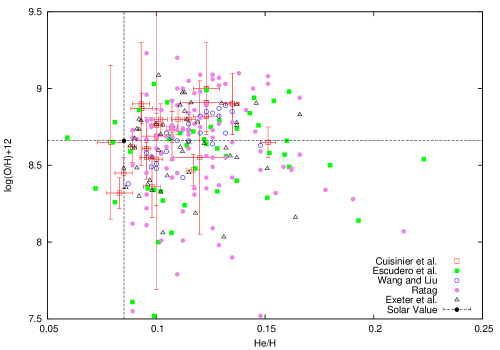
Figure 4: The figure shows abundances of log(O/H)+12 as a function of He/H. The red open squares, green filled squares, blue open circles, violet filled circles and black open triangles are from the GB-PNe data from (cui00) (Cuisinier set), esc04 (Escudero set), liu01 and wl07 (Wang & Liu set), rat92; rat97 (Ratag set), and ex04 (Exeter set), respectively. For reference the solar values of asp05 are indicated by the dashed lines.

Overall each of the data sets seem to agree with each other, however, there are some important differences. Most of the points from the different sets seem to fall in the same area on the graph. For He/H values between $\sim 0.08$ and $\sim 0.14$ the values of O/H for all of the sets overlap although some of the sets have a larger scatter. The Escudero and Ratag sets have the largest scatter in O/H and the Cuisinier and Wang & Liu sets have the smallest. The biggest difference is both the Escudero and Ratag sets have a tail of GB-PNe with He/H greater than 0.16, whereas, the other sets do not.

What is the origin of the high He/H tail in Figure 4? In this figure for He/H$\ga 0.150$ the value of O/H decreases from a maximum and appears to level out into a tail. This tail is composed of PNe from only two of the sets, the Escudero and Ratag sets. Since this tail does not show up in the other sets, this suggests the most likely explanation is due to either differences in how PNe were selected or how the abundances are computed. The abundances for all five sets were computed using similar sets of ionization correction factors and they produce very similar results in the He/H range of 0.08 to 0.14. This suggests the differences arising from the methods of calculating the abundances are small. This does not rule out errors in computing He/H as an explanation. A possible origin of this tail is in the GB-PNe selection criteria. The different sets use different methods to determine what is a likely GB-PNe. For example for the Cuisinier set the criteria for a PN to be in the bulge are (i) its diameter must be smaller than 10 arcsec, (ii) it must be within 5 degrees of the galactic centre, and (iii) the 6cm radio flux must be less than 100 mJy. The Escudero set selected for GB-PNe as PNe within 5 kpc of the centre. This is a less discriminating criteria and as a result a larger fraction of the Escudero set being disc PNe. esc04 estimates $\sim 20$ percent of their sample is disc PNe. A possible explanation of the tail is it consists of inner disc PNe from intermediate-mass progenitors. For purposes of modeling it will be assumed this tail is not real since it should show up in all five sets.

There are a couple of possibilities if this tail is real bulge population. One possibility is it is produced by low-mass progenitors with $Y\sim 0.4$. This is not unprecedented since some globular clusters may contain a third, even more helium rich (extreme) population. Another alternative is these PNe would be the progeny of galactic bulge blue straggler stars (cl11). The blue stragglers in the bulge with an assumed MSTO at 1.4$\,{\rm M}_{\sun}$ could be as massive as 2.8$\,{\rm M}_{\sun}$. Stars of that mass would experience many TDU events which would enhance the abundances of helium and carbon; this could explain the high He abundances. Blue straggler models for the tail would probably also require enhanced helium abundances since material from the interior of the star being consumed would end up near the surface.

Is there a relationship between O/H, which stands in for metallicity, $Z$, and He/H which stands in for the helium mass fraction, $Y$? In Figure 4, by visual inspection, it appears that as O/H increases so does He/H in the range of He/H of 0.08-0.14. This trend is much clearer in Figure 5 where only the sets with the smallest scatter, the Cuisinier set and Wang & Liu sets, are plotted. In Figure 5 there is a clear trend that as O/H gets larger so does He/H in the He/H range from 0.08 to 0.135. The Escudero and Exeter sets do not show as a clear relationship between O/H and He/H as the Cuisinier and Wang and Liu sets. However, both sets are consistent with there being a relationship between O/H and He/H, as there appears to be an upward trend in both. The Ratag sample is noisier then the other samples, but it is consistent with there being a relationship between O/H and He/H.

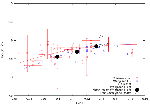
Figure 5: This figure is the same as Figure 4 but with only the Cuisinier and Wang & Liu sets only. The solid and dotted lines are respectively the fits to the Cuisinier and Wang & Liu set. The large filled circles are the parameters fit by TP-AGB stars modeled to the Wang & Liu fits in 4.1. The large open triangles are the positions of fits of additional models in LABEL:sec:lc, LABEL:sec:ml, and LABEL:sec:ho. See the text in Section 4 for an explanation.

An important point to note is there may be a systematic difference between the abundances of oxygen as determined from unevolved stars and PNe. chi09 compared the oxygen abundances of GB-PNe determined from CELs to the oxygen abundances determined from giants and found the PNe abundances are systematically lower by 0.3dex. The origin of this shift is not clear since dust should, at most, decrease the abundance by $\sim 0.1$dex. It is not clear if this shift is real or not so the models in LABEL:sec:ho will look at both possibilities.

Does O/H actually trace O/H of the progenitor star? The abundance of oxygen in a PN should be close to but not identical to the progenitor ZAMS abundance, since oxygen should experience a slight decrease (typically a few percent) in abundance during the FDU at low masses. At higher masses, which we will not look at in this paper, oxygen is decreased by the SDU and HBB. Oxygen can be increased in TDU events. However, all of these changes cause only minor changes in the abundance of oxygen, so the oxygen abundance in PNe should be a good indicator of the ZAMS oxygen abundance even with high mass progenitors.

Additional support for the proposition He/H increases with metallicity comes from plotting He/H against heavy elements other than oxygen. Figure 6 shows Ne/H, S/H, Cl/H and Ar/H as a function of He/H. This figure shows clearly for all the sets abundances of Ne, S, Cl and Ar increase with He/H up to He/H$\sim 0.14$. None of these elements is thought to be significantly effected by the stellar evolution between ZAMS and the PN stages. Neon and argon have an additional advantage, because they are noble gases, thier abundances will not be affected by being drained onto dust grains, although for the other elements this effect is probably small. This figure suggests as the metallicity of the star increases so does the value of He/H. For all four elements the abundances increases with He/H up to He/H$\sim 0.14$. There is a tail at high He/H where these abundances drop off. This is the same pattern as seen for the relationship between the abundance of oxygen and He/H. The high He/H tail show up in each graph where the Escudero and Ratag sets were plotted. As noted above its existence is questionable.

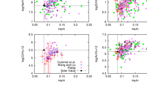
Figure 6: The figure shows abundances of log(Ne/H)+12, log(S/H)+12, log(Cl/H)+12, and log(Ar/H)+12 as a function of He/H. The symbols have the same meaning as they do in Figure 4.

In this paper it is assumed the most metal rich PNe are due to the youngest progenitors. These youngest and most massive progenitors seem to have a PN He/H between 0.130 and 0.140 and the abundance of oxygen is in the range 8.80-8.90. If we accept the potential systematic upward shift of the oxygen abundance by 0.3dex then the oxygen abundance could be approximately 9.10-9.20 for the most metal rich PNe. In Section 4 these will be the abundances of the most massive GB-PNe matched.

Does it matter if there is a injective relationship between metallicity and He/H or if there is a spread of metallicities for the same $Y$ value? The answer is no since there are a significant number of GB-PNe with He/H$\approx 0.14$ in all five sets which require some explanation. The $Y$ values of PNe can be estimated from the following formulas

$$X+Y+Z=1$$ (18)

and

$$\frac{Y}{X}=4{\rm He/H}.$$ (19)

A maximum $Y$ values can be estimated by assuming the GB-PNe with the highest He/H have $Z=0.02$. In this case for He/H=0.140 the formulas above give $Y\approx 0.35$. Different, but reasonable assumptions about $Z$ would not appreciably change $Y$. Clearly the GB-PNe span a significant range of possible $Y$ and $Z$ values.

In this paper it is assumed that each value of the progenitor $Z$ gives a unique value of $Y$. To get a relationship between O/H and He/H quadratic fits have been made in Figure 5 to the Cuisinier set and the Wang & Liu set. The fit to the Cuisinier set is given by

$$log(O/H)+12=-103.981({\rm He/H})^{2}+32.4351({\rm He/H})+6.35192.$$ (20)

The fit to the Wang & Liu set is given by

$$log(O/H)+12=-97.2275({\rm He/H})^{2}+30.9835({\rm He/H})+6.42915.$$ (21)

If He/H=0.130 the value of O/H is respectively 8.81 and 8.81, respectively, for the Cuisinier and the Wang & Liu sets. At He/H=0.09, O/H is respectively 8.43 and 8.43 for the Cuisinier and the Wang & Liu sets. Some of the models of the PNe global parameters from models will be made along these fits but some fits will be made away from these curves.

3.2 Central star masses of GB-PNe

The mass of the central star of a PN (CSPN) is critical for determining the mass of the progenitor. Both observational (wei77; wei00; kal05; cat08) and theoretical studies (dom99; mar01; mch08) indicate there is a link between the mass of the progenitor and the mass of the resulting white dwarf. The expected theoretical relationship is qualitatively confirmed by the observational studies which show the larger the mass of the progenitor the larger the mass of the resulting white dwarf. Theoretical studies indicate the initial-final mass relationship (IFMR) should depend on metallicity. In particular, the smaller $Z$ is the larger the resulting white dwarf for any given ZAMS mass. Any potential metallicity relationship is less clear in the observational studies (cat08) as there is considerable scatter in the observational IFMR. Other factors such as stellar rotation may also affect the IMFR (dom96; cat08).

In Paper I it was predicted there should be a difference in the IFMR for different ZAMS value of $Y$. Given the same mass and metallicity a higher value of $Y$ gives a higher core mass at the onset of the first thermal pulse. Since the core mass at the first pulse is correlated to the CSPN mass, a higher $Y$ on the ZAMS should lead to a larger CSPN mass.

There do not appear to be a large number of recent studies on the CSPN masses of GB-PNe. The existing studies are consistent with the expectation the bulge contains mostly low-mass ZAMS progenitors. tyl91 used a variety of methods to get the CSPN mass; this included plotting the Zanstra luminosities of PNe, L(HI) and L(HeII) as functions of the respective Zanstra temperatures, T(HI) and T(HeII). These were compared to the theoretical CSPN tracks of sch81; sch83 to get the CSPN masses. tyl91 also compared the visual magnitudes of the CSPN to the expansion ages and the temperatures to their $f$ parameter to get CSPN masses. They got an average mass of the Galactic bulge CSPN of $0.593\pm 0.025\,{\rm M}_{\sun}$. Their Figures 11 and 12 present the CSPN mass distribution of all their masses and all the best determined masses, respectively. There is a peak in both figures of the number of CSPN masses at $\sim 0.58\,{\rm M}_{\sun}$. The distributions tails off quickly to $0.65\,{\rm M}_{\sun}$. About 10 percent of their sample have masses greater than 0.62$\,{\rm M}_{\sun}$ in their sample. This is nearly the same as their estimate of the number of disc objects contaminating the sample (st91). The high mass tail could be due to sample contamination by foreground objects or could be due to blue stragglers in the bulge. This study suggests the highest mass CSPNs have masses between 0.58 and 0.62$\,{\rm M}_{\sun}$.

ratagphd determined the luminosities and temperatures by two methods. The first is a version of the Zanstra method which adds in the energy from the far infrared part of the spectrum to get the stellar temperature and the luminosity. The second is a method using an photoionization model where important line ratios were matched to observations to get the spectral distribution of the stellar continuum The stars’ effective temperature is derived from the continuum. The luminosity in the second method is determined by adding the energy from all emission lines, the free-free emission and the infrared luminosity and the portion of the stellar spectrum emitted with wavelength less than $91.2\,{\rm nm}$. The agreement between the luminosities and temperatures determined by various methods is pretty good (See Figure 2 and Figure 4 in ratagphd Chapter 4 for these comparisons.).

ratagphd plotted these luminosities and temperatures on HR diagrams with theoretical tracks. This figure is partially duplicated in Figure 7. Almost all the Ratag PNe fall between the $0.546\,{\rm M}_{\sun}$ and the $0.644\,{\rm M}_{\sun}$ tracks. However, the majority falls between $0.546\,{\rm M}_{\sun}$ and $0.600\,{\rm M}_{\sun}$. This suggests the most massive GB-PNe CSPN are between 0.58 and 0.60$\,{\rm M}_{\sun}$. This is consistent with the tyl91 results.

Figure 7: This figure shows the positions of the Ratag set on the HR diagram with the theoretical vw94 put in for comparison. The filled squares are the PNe with He/H$<0.120$ and the open squares are the PNe with He/H$>0.120$. The solid, long dashed, short dashed, dotted, long dash-dot, and short dash-dot are the theoretical tracks of 0.569, 0.597, 0.633, 0.677, 0.754, and 0.900$\,{\rm M}_{\sun}$. All the tracks have ZAMS $Z=0.016$.

Both the tyl91; ratagphd results suggest that the progenitors of the GB-PNe are relatively low-mass since the observed CSPN masses are low. Both of these studies are quite old and neither has been repeated recently so some skepticism is justified. However, the distance to the bulge is relatively well known and the intensity of the radiation from the GB-PNe can be measured with some confidence. Many of these PNe appear to fall on the horizontal part of the CSPN tracks. Since the luminosities, which are nearly constant in this region, can be fairly well constrained, the CSPN masses should be reasonably accurate ($\Delta{\rm M}_{\rm CSPN}\sim 0.03\,{\rm M}_{\sun}$).

Some additional support for a low maximum bulge CSPN masses comes from the luminosity of the tip of the AGB branch. zo03 found the maximum bolometric magnitude of the AGB tip is -5.0 which corresponds to a luminosity of about $8000\,{\rm L}_{\sun}$ ($\log{L}\approx 3.9$). In Figure 28 of zo03 most of the stars at the tip of the AGB are closer a bolometric magnitude of -4.5 which corresponds to a luminosity of about $5000\,{\rm L}_{\sun}$ ($\log{L}\approx 3.7$). If you compare these luminosities to the horizontal parts of the CSPN tracks of bl95 this implies a CSPN mass $\sim 0.605\,{\rm M}_{\sun}$ track. Therefore, the AGB tip luminosity suggests the majority of the CSPNs have masses less than $0.61\,{\rm M}_{\sun}$.

Putting all of the evidence together suggests the most massive CSPN PNe in the bulge are between 0.58 and 0.62$\,{\rm M}_{\sun}$. Therefore, for the purpose of model fitting in this paper, it is assumed all the masses of the CSPN of GB-PNe are less than or equal to $0.620\,{\rm M}_{\sun}$. This maximum mass may be less than $0.600\,{\rm M}_{\sun}$.

Another study which looked more recently at the question of bulge CSPN masses is hul08. In this study the spectra of the central stars of a small sample of GB-PNe was obtained. From these the abundances, the effective temperatures, and the surface gravities were obtained. The effective temperature and surface gravity were compared to theoretical tracks to get the CSPN mass. Using this method a higher average mass is obtained for their small sample (5 objects) of PNe of $0.696\,{\rm M}_{\sun}$, which is higher than studies which measure the effective temperature and luminosity using the nebula. Two of the GB-PNe have a mass of nearly $0.800\,{\rm M}_{\sun}$ which implies intermediate-mass progenitors (M$\ga 3.5\,{\rm M}_{\sun}$). There is reason to be skeptical of this though. As the authors note, if their inferred luminosities are used to find the distance to the Galactic bulge is $10.7\pm 1.2\,{\rm kpc}$. This distance which is 25 percent larger than the typical determination, e.g. $8.4\pm 0.4\,{\rm kpc}$ (gh08).

What is the relationship between the helium abundance and the CSPN mass of the the GB-PNe? In Figure 8 the five different samples of GB-PNe He/H are plotted as a function of their CSPN mass from tyl91. Visual inspection of this figure indicates there is a lot of scatter in all sets but the graph is consistent with an upward trend between $0.55$ and $0.62\,{\rm M}_{\sun}$. If there is an upward trend it appears to end between 0.60 to 0.63$\,{\rm M}_{\sun}$. The lack of a significant correlation could be due to the relatively large errors expected in the individual CSPN masses. A positive correlation between He/H and CSPN mass would be expected if as might be expected in any typical chemical evolution model where the ISM is being simultaneously enhanced in both helium and metals. Therefore the more massive CSPN should have higher values of $Y$ and $Z$.

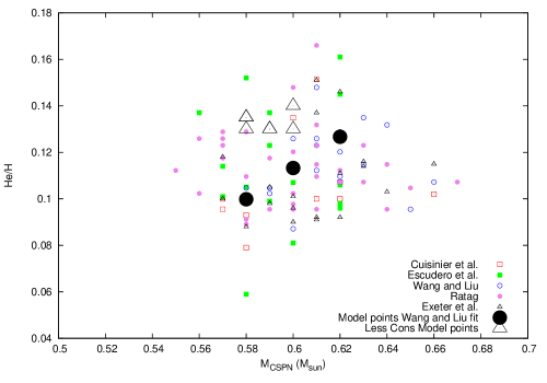
Figure 8: The figure shows the value of He/H for GB-PNe versus the central star mass from tyl91. The symbols have the same meaning as in Figure 4. The large filled circles and large open triangles have the same meaning as in Figure 4

At even higher core-masses it appears the value of He/H drops off into a tail with a relatively modest He/H ($\sim 0.110$). Is the high CSPN core mass ($\ga 0.62\,{\rm M}_{\sun}$) tail real effect in the bulge or is it due to disc PNe contamination? Although this paper can not definitively answer this, the fact most of the sets have similar He/H in the tail part of the distribution suggests the tail may be real. What might cause this tail? If it is real then one possibility is these are foreground objects misidentified as bulge objects. If they are disc objects they would appear more luminous and thus more massive. If they are foreground objects then these PNe would have values of He/H typical of the disc PNe (He/H$\approx 0.110$). Another possibility is these objects are the progeny of blue straggler star in the bulge. Potential blue stragglers have recently been identified in the bulge and the progeny of these more massive stars would be more massive CSPN.

To get a better look at the relationship between core mass and He/H from the various GB-PNe of the Escudero set and the Wang & Liu set are plotted as a function of CSPN mass, where the CSPN masses are from the best set from the tyl91 paper (as identified in that paper), in Figure 9. Both of these sets seem to show as CSPN mass increases so does the value of He/H. This does not mean there is a unique relationship between CSPN mass and He/H. Only the fit to the Wang & Liu set has a truly significant correlation coefficient. The lack of a definite relationship could be due to the significant scatter in the CSPN masses.

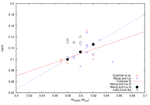
Figure 9: The figure is the same as Figure 8 but only the Cuisinier and Wang & Liu sets are plotted against the best CSPN masses of tyl91. Linear fits to both sets are shown to make the trends are clear.

Although there is possibly no unique relationship between He/H and CSPN mass this paper will assume there is one. The Wang & Liu set seems to have the clearest relationship between He/H and CSPN mass. The fit to the Wang & Liu set is given by

$${\rm He/H}=0.671821({\rm M}_{\rm CSPN}-0.60)+0.113244.$$ (22)

This equation will be used to derive the parameters to be fit in Section 4.1.

In Figure 7 the Ratag sample is separated into two samples with high He/H ($>0.120$) and low He/H ($<0.120$) and plotted on the HR diagram using the Ratag values of $\log{L}$ and $\log{T_{eff}}$. This is done since this gives a larger set of CSPN masses than the tyl91 CSPN masses. Visual inspection reveals there is at most a minor difference in the distribution on the HR diagram of the two subsets. More of the high He/H GB-PNe seem to fall on the cooling part of the tracks. This indicates the high He/H PNe a slightly higher CSPN mass, since more massive CSPN evolve more quickly (e.g. see vw94). This makes it more likely more massive CSPN will end up on the cooling part of the tracks.

3.3 Helium versus N/O in GB-PNe

Nitrogen is a very important element in PNe since it is often used as an indicator of nuclear processing of material in the interior. This material is then transported to the surface via convection. In low and intermediate-mass stars nitrogen is typically enhanced at the FDU and SDU. Nitrogen can also be enhanced when CNO process occurs at the base of the convective envelope in AGB stars, known as HBB.

Bulge stars are thought to be fairly low-mass, the work of ben10; ben11 suggests the youngest stellar ages are $\sim 3\,{\rm Gyr}$ of age which would suggest a maximum MSTO mass of $\sim 1.5\,{\rm M}_{\sun}$. Stars of this mass should only experience the FDU which has only a limited effect on N/O, typically doubling N/O, which is an increase of about 0.3 dex. For a ZAMS star with a solar ratio of N/O this would mean N/O would be around 1/3 ($\log{\rm(N/O)}\approx-0.5$) in a PNe.

In Figure 10 the ratio of N/O of GB-PNe is plotted as a function of the ratio He/H for all five sets. There is clearly a relationship between N/O and He/H for GB-PNe, with both increasing at the together in all of the sets. A fit to the Wang & Liu set, which is shown on the figure gives:

$$\log{\rm N/O}=15.25({\rm He/H}-0.100)-0.755.$$ (23)

This line appears to be a good fit to all of the data sets. It will be adopted to determine the GB-PNe N/O parameter to match in some cases.

Of particular importance is the fact the highest N/O ratios are $\la 1$ in almost all of the sets. The Cuisinier and Wang & Liu sets all of the GB-PNe have N/O$\la 1$. For the Exeter set with the exception of two clear outliers with N/O$\approx 10$, all the GB-PNe N/Os in their sample are $\la 1$. The Escudero set has only a two PNe with N/O significantly larger than 1. Only the Ratag set has a significant number of GB-PNe with N/O$\ga 1$. For purposes of this paper it will be assumed for GB-PNe N/O$<1$ since all sets have points in this range and most of them do not have a significant number of GB-PNe with N/O significantly larger than 1.

An N/O of $\sim 1$ suggests either the progenitors are intermediate-mass or else are low-mass with a higher than solar N/O ratio, 0.13. The second is very interesting since it would suggest the gas from which these stars formed was enhanced in both helium and nitrogen. This would indicate the bulge ISM was enhanced by the products of CNO burning.

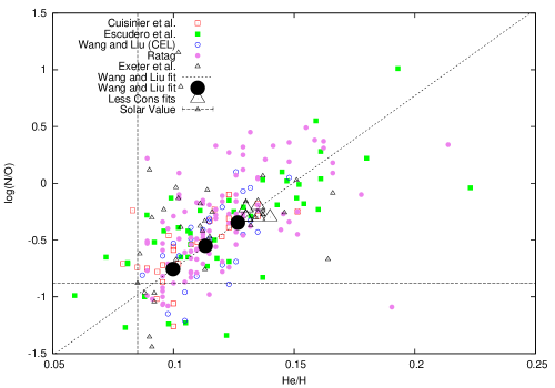
Figure 10: This figure shows the positions of the values N/O as a function of He/H for the GB-PNe. The symbols have the same meaning as in Figures 4 and 5.

3.4 Carbon in GB-PNe

Another very important element is carbon. Information about this element for GB-PNe is limited because the bulge is heavily reddened, and the most reliable lines for determining the carbon abundance in PNe are in the ultraviolet. The Wang & Liu set contains a limited number of measurements of the ratio of C/O from both CELs and ORLs. Most of their C/O ratios from both methods are below 1 but there are a small number with ${\rm C/O}>1$ which could indicate TDU events. This is consistent with the findings of gu08; pc09; st12 who found the majority of GB-PNe have oxygen-rich dust spectrum but there is a minority of stars ($\approx 10$ percent) which have carbon-rich dust spectrum. A large fraction ($\approx 40$ percent) of GB-PNe have a mixed dust spectrum with both carbon and oxygen features. The mixed features may be associated with a TDU event occurring near or after the transition from an AGB star to a PN, but it may also be due to a dense torus around the progenitor where, during the transition from the AGB to PN phases, chemical reactions occur in an oxygen rich environment which produces poly-aromatic hydrocarbons (PAHs). This PAH production shows up as the carbon-features in a mixed dust spectrum (guz11). In the second scenario a mixed feature spectrum does not necessarily indicate a carbon-rich star in which a TDU occurred.

The conclusion is the majority of progenitors of GB-PNe do not experience a TDU event. This is supported by the lack of bright carbon stars in the bulge (alr88). This indicates the carbon stars in the bulge which do exist probably formed as the result of a mass transfer in a binary system and not by the action of the TDU. This further supports the idea that the stars in the bulge are older, since only stars with M$\la 1.6\,{\rm M}_{\sun}$ do not experience a TDU.

There may be some indication that a minor amount of TDU occurs. utt07 observed Tc in bulge AGB stars which is an indication of the action of the TDU. In their spectra Tc was only observed in the brightest and reddest stars with the longest periods indicating they are probably the most evolved and closest to the transition to the PN phase. This suggests that the youngest stars in the bulge may be just massive enough to experience one or two dredge-ups before entering the PN phase. Depending on the mass of the residual envelope an AGB star could become a carbon star at the last moment. This would agree with the small number of GB-PNe with ${\rm C/O}>1$. From their luminosities utt07 concluded that the progenitors of these Tc rich stars are $\approx 1.5\,{\rm M}_{\sun}$.

All indications are the TDU plays only a minor role in modifying the abundances in PNe. This is important since the TDU can significantly modify the abundance of helium but it takes several TDU events to significantly modify it. Therefore, He/H for these lower mass models is mostly a function of the initial value of He/H and the result of the FDU. It will be assumed for fitting purposes, the C/O for GB-PNe is less than 1.

4 Results

In the previous section it was noted there are a range of possible GB-PNe parameters to fit. In this section models are calculated which fit different potential but reasonable parameters of the highest mass CSPN. The first set of GB-PNe parameters fit in this paper is defined by the Wang & Liu fits. This set shows the most well defined trends and it seems to be a reasonable fit. After that this paper will look at some less conservative possibilities where the maximum bulge CSPN mass is less than $0.62\,{\rm M}_{\sun}$.

The basic fitting technique is as follows. A set of typical PNe parameters to fit is chosen. These parameters are the assumed CSPN mass and the PNe values of He/H, O/H, and N/O. The ZAMS mass, [Fe/H], $Y$ and N/O were chosen and a model run. The ZAMS parameters were modified until a fit to the PNe parameters was acheived.

4.1 Wang & Liu set

In this subsection models are matched to points on the fits to the Wang & Liu set. These fits were chosen since this set shows the most well defined trends. There is also a defined trend in CSPN mass, which will be used to explore the chemical evolution of the bulge. Table 4 shows the PNe parameters fit, the ZAMS parameters of the best fitting models. The positions of the GB-PNe parameters to be fit are indicated in Figures 5, 10 and  9. In these fits the most massive CSPN fit have a mass of $0.62\,{\rm M}_{\sun}$. This probably too high maximum CSPN mass will produce the largest bulge progenitor mass. The top of the trend was fixed at a CSPN mass of $0.62\,{\rm M}_{\sun}$ in the fits to the Wang & Liu GB-PNe this will produce an He/H $\approx 0.130$ which is similar to the maximum He/H in GB-PNe as defined in Subsection 3.1. The lowest mass models have a CSPN mass of $0.56\,{\rm M}_{\sun}$.

Table 4: Parameters to fit and parameters of model fit for Wang & Liu set

CSPN mass	He/H	log(O/H)+12	log(N/O)	M	$Y_{ZAMS}$	$Z_{ZAMS}$	[Fe/H]	log(N/O)${}_{ZAMS}$
0.58	0.09981	8.553	-0.559	1.43	0.257	0.0087	-0.18	-0.800
0.60	0.11324	8.691	-0.400	1.63	0.293	0.0122	0.003	-0.630
0.62	0.12668	8.794	-0.347	1.80	0.320	0.0175	0.195	-0.573

The CSPN mass, He/H, log(O/H)+12, and log(N/O) are the PN parameters being fit. M, $Y_{ZAMS}$, $Z_{ZAMS}$,[Fe/H] and N/O${}_{ZAMS}$ are the model ZAMS parameters of the best fitting model. In all of these models the parameter $k_{1}$=[$\alpha$/Fe] is set as +0.35. The end of the alpha plateau, $k_{2}$=[Fe/H], is set to -1.