1 Introduction

This paper is essencially motivated due to the J-PAS project http://j-pas.org, which in a near future will produce 8000 sq degrees of imaging in 56 filterbands of 135Å up to magnitude $i_{AB}\approx 24$. The survey, besides producing a very high-quality photometric redshift catalog, will provide highly informative data important to other astronomical communities as galaxy evolution.

Here we describe a bayesian method to “boost the spectral resolution” of these kind of photometric data. The idea, which will be described in more detail on section 3, is basically that if a high-resolution degrated spectra (or a set of them) is similar to an observed j-spectra then its physical properties (and even emission lines) would be similar.

To test the efficiency of this method, we used the starlight-SDSS [2] http://starlight.ufsc.br/ database as a sandbox. We downloaded the 926246 galaxies where there are measured physical properties and emission lines.

2 From SDSS to JPAS

Given a SDSS observed spectra, one can convert its energy distribution $O_{\lambda}$ to an arbitrary observed photometric filter $l$ defined by its transmission curve $T_{l,\lambda}$ using the simple conversion $J_{l}=\frac{\int O_{\lambda}T_{l,\lambda}d\lambda}{\int T_{l,\lambda}d\lambda}$ and the error on the filter $l$, $\sigma^{2}(J_{l})$, with the relation $\sigma^{2}(J_{l})=\Lambda_{l}\langle\sigma(n_{\lambda})^{2}t_{l,\lambda}^{2}\rangle\Delta\lambda$ where $\Lambda_{l}\equiv N_{\lambda,l}\Delta\lambda$ is the effective filter size and $n_{\lambda}$ is the spectral error in each point.

The filtersystem curves to JPAS considering an airmass of 1.3 and the expected CCD plus Telescope efficiencies are shown on figure 1. There will be 56 filters, but due to the spectral coverage of SDSS we removed the first one in the blue and the four last filters giving us an filtersystem of 51 filters plotted in solid lines. For comparsion, we plotted right below our filtersystem the SDSS filterset u, g, r, i and z sensitivities through the same air mass.

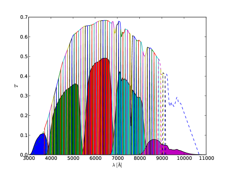
Figure 1: JPAS 56 filtersystem sensitivity curves. The 51 solid lines are the filters used on this work assuming mirror and CCD characteristics and an airmass of 1.3. We also plotted in solid fill the SDSS u, g, r, i and z filters in the same conditions.

The main idea of this work is to obtain high precision properties from low resolution data by taking a shortcut from what we measure from high resolution spectra. We consider that if an pair object-template j-spectra are similar, then their measured properties will be similar as well. On fig 2 we show two examples of matching two objects with their five best matches in respect to our template library library. In green we plotted the SDSS object and in blue its four best matches accordingly to their $\chi^{2}$ calculated over their j-spectrum (plotted as red dots). On the right panel we have an example of a star-forming galaxy and on the left an early-type.

This idea is similar to the adopted by [5] and [6] and others, but with an important difference: Here we do not compare an observed spectrum with a set of models but we compare it to a set of another observed spectra. This not only permits us to measure the standard physical properties such as mean age and stellar masses that can be measured by ohter methodos, but it also allows us to measure indirectly emission lines on data which we evidently do not have enough resolution. This is the most relevant advantage of this method.

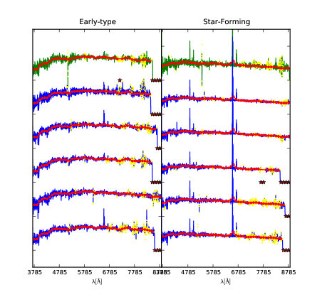
Figure 2: Two examples of j-spectrum and its 5 best matches based on $\chi^{2}$. At the top, in green, the two observed spectra examples: an early-type on left panel and a star-forming galaxy on the the right. In blue, from top to bottom, the first five best matches. Their j-spectrum is represented by the connected red dots. Yellow points are flagged as bad pixels and were not considered. Stars represent the points were j-spectrum is not available.

3 Method

To derive the properties $p$ listed down on table 1, we calculated for 100k objects and two samples of comparsion their likelihood functions ${\cal L}_{i,j}=e^{-f_{L}\frac{1}{2}\chi^{2}_{i,j}}$. Where $\chi^{2}_{i,j}=\sum_{l}\frac{1}{N_{\rm good}}(O_{l,i}-a_{i,j}B_{l,j})^{2}w_{l,i,j}^{2}$ with a scaling factor $a_{i,j}=\frac{\sum_{l}O_{l,i}B_{l,j}w_{l,i,j}^{2}}{\sum_{l}B_{l,j}^{2}w_{l,i,j}^{2}}$ which is determined by interacting the calculation of $a$ and $\chi^{2}$ until a convergence critery of $\Delta a_{i,j}<10^{-5}$ is accomplished. In our simulations, this takes no more than four interactions. The $f_{L}$ term adjusts the width of the PDF. It can be adjusted to minimize errors, but we will not treat it here.

The weighting used to the spectra was defined by $w^{2}_{l,i,j}=\left(\frac{\langle O^{2}_{l,i}\rangle}{O^{2}_{l,i}}\right)\left(\frac{1}{\sigma^{2}(O_{l,i})+a^{2}_{i,j}\sigma^{2}(B_{l,i})}\right)$. This was selected to have an unbiased weight in the amplitude of the spectra. In other words, we would like to give the same importance to the parts with high fluxes (e.g. emission lines) than that to that regions that have lower ones (e.g. continuum).

With the likelihood for each object and base, we calculated as the output of our method a PDF estimator. In our case, to estimate the output, we used the likelihood-weighted average $\overline{p_{i}}=\frac{\sum_{j}p_{j}{\cal L}_{i,j}}{\sum_{j}{\cal L}_{i,j}}=p_{out,i}$

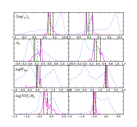
Figure 3: Examples of normalized PDF distributions to age, extinction, H$\alpha$ and [N ii]/H$\alpha$. The left and right boxes corresponds to the left and right observed galaxaies shown on fig. 2. In blue dashed line we show the distribution of our base of templates, in magenta the likelihood distribution (or the posterior) and the horizontal lines represents in solid black the 16th and 84th percentiles, in red dashed the average and in solid green the value measured by starlight directly on the spectrum.

4 Sample selection

Our main sample was retrieved from the starlight-SDSS database based on very wide criteria, trying to get all kinds of objects. Firstly, we separated from the database the galaxies which were in the SDSS main galaxy sample [7], then we selected those who do not have any bad pixel in intervals of 31Å centered on the emission lines H$\alpha$, H$\beta$, [N ii]$\lambda$6584, [O ii]$\lambda$3727 and [O iii]$\lambda$5007 to assure that when we do not measure an emission line it is because it is too weak to measure and not because of any observational error. A last selection in redshift ($0.01\leq z\leq 0.11$) was applied in order to have spectral coverage on the wavelength interval where JPAS will observe. Those criteria reduced the total number of galaxies on our sample from 926246 to 299253 galaxies. All these galaxies were corrected to the rest-frame. As a quick-look test, we will not treat the redshift as a variable here and all results will be shown to $z=0$.

We then converted all the observed spectra to J-spectra. In case of problems on the SDSS spectra (e.g. bad pixels), we changed the observed flux to the best fit from the starlight in the cases where the filters have less bad pixels than 50% of the filter width. Otherwise, the filter is flagged to be neglected.

Then, we divided the sample in two sub-samples: one with the galaxies with $S/N>20$ (113821 galaxies) which we call mother library and other one with galaxies with $S/N<20$ (185432 galaxies) which we call object sample. All comparsions made in this paper will be in respect of a set of objects and their PDFs calculated over a given library which is a set of galaxies from the mother library. From the mother library, we selected two samples of galaxies based on two independent diagrams.

The first one, which we call CMD, is based on the physical analog to the color-magnitude diagram to galaxies, the $\log\ M_{\star}$ – $\langle\log\ t\rangle$ diagram. We chopped this diagram in boxes of 0.1 dex, and on each box we got 10% of the objects distributed along the $A_{V}$ axis. This gives us 11952 galaxies on this library.

The second library, which we call WHAN, is based on the WHAN diagnostic diagram introduced by [3] and divide the galaxies basically between star-forming, active nuclei and passive or retired galaxies. We did the same cut on this diagram as we did on CMD library, but here we changed the $A_{V}$ to the emission line ratio $\log[\rm{N}\,\textsc{ii}]/{\rm H}alpha$. This gives us 27537 galaxies on this library.

5 Results

To estimate our method’s precision, we compared the properties derived by our method (output) on the low-resolution j-spectra with the values derived using starlight on the high-resolution SDSS spectra (input). So, to do this comparsion, we evaluate, for each property $p$ and object $i$, the $\Delta p_{i}=p_{i,\rm output}-p_{i,\rm input}$.

This experiment shows the potential of the proposed method and accomplish with our initial objective which is to test the precision of galaxy properties with it. From table 1, we can resume the precision of our method: It can measure physical properties like age and extinction with typical precision of $0.2$ dex (or mag, in the case of $A_{V}$) and emission lines with $0.3$ dex and our library selection does not affected the final result, probably because we have a number of templates which are in both libraries and/or beacause we have oversampled libraries with $N_{\rm galaxies}$ of about 10k galaxies.

Once more, our main result is that we can measure emission lines without having sufficient spectral resolution to do it directly on our data.

Table 1: Results

Property	$\overline{\Delta p}$	$\sigma(\Delta p)$ (CMD)	$\overline{\Delta p}$	$\sigma(\Delta p)$ (WHAN)
$A_{V}$	0.023	0.106	0.023	0.101
$\langle\log t_{\star}\rangle_{L}$	-0.018	0.199	-0.013	0.192
$\langle\log Z_{\star}\rangle_{L}$	-0.021	0.144	-0.020	0.141
$\log M/L_{r}$	-0.045	0.114	-0.040	0.110
$\log W_{[O_{II}]}$	0.051	0.223	0.040	0.218
$\log W_{H\beta}$	0.024	0.145	0.030	0.143
$\log W_{[O_{III}]}$	0.046	0.245	0.029	0.232
$\log W_{H\alpha}$	0.010	0.160	0.022	0.157
$\log W_{[\rm{N}II]}$	-0.028	0.159	-0.010	0.156
$\log[N_{II}]/H_{\alpha}$	-0.045	0.141	-0.044	0.146
$\log[O_{III}]/H_{\beta}$	0.026	0.250	-0.000	0.238
$\log H_{\alpha}/H_{\beta}$	-0.011	0.107	-0.010	0.114
$\log S_{II}/H_{\alpha}$	-0.006	0.172	-0.016	0.174
$\log[O_{II}]/H_{\beta}$	0.036	0.202	0.016	0.198
$\log[O_{III}]/[N_{II}]$	0.075	0.265	0.044	0.252

References

- [1] Benítez, N., 2000, ApJ, 536, 571
- [2] Cid Fernandes R. et al, 2005, MNRAS 358, 363
- [3] Cid Fernandes R. et al, 2010, MNRAS, 403, 1036
- [4] Driver, S. P, 2011, arXiv:1112.6244
- [5] Gallazzi, A. et al, 2005, MNRAS 362, 41
- [6] Kauffmann, G. et al, D., 2003, MNRAS, 341, 33
- [7] York, D. G et al, 2000, AJ, 120, 1579