Generation of twist on magnetic flux tubes at the base of the solar convection zone

Using two-dimensional magnetohydrodynamics calculations, we investigate a twist generation mechanism on a magnetic flux tube at the base of the solar convection zone based on the idea of Choudhuri, 2003, Sol. Phys., 215, 31 in which a toroidal magnetic field is wrapped by a surrounding mean poloidal field. During generation of the twist, the flux tube follows four phases. (1) It quickly splits into two parts with vortex motions rolling up the poloidal magnetic field. (2) Owing to the physical mechanism similar to that of the magneto-rotational instability, the rolled-up poloidal field is bent and amplified. (3) The magnetic tension of the disturbed poloidal magnetic field reduces the vorticity, and the lifting force caused by vortical motion decreases. (4) The flux tube gets twisted and begins to rise again without splitting. Investigation of these processes is significant because it shows that a flux tube without any initial twist can rise to the surface in relatively weak poloidal fields.

1 Introduction

Surface sunspots are the most prominent feature of solar activity. It is thought that the magnetic flux is generated by the dynamo action of the differential rotation at the base of the convection zone (Parker, 1955; Choudhuri et al., 1995; Dikpati & Charbonneau, 1999; Hotta & Yokoyama, 2010a, b). The magnetic flux rises to the surface owing to the magnetic buoyancy and generates sunspots on the surface.

In observational and theoretical assessments, this magnetic flux is thought to be twisted. On the surface, vector magnetic field observations have revealed that the solar active regions have a statistically significant mean twist (Pevtsov et al., 1995, 2001, 2003). The quantity $\alpha\equiv\langle J_{z}/B_{z}\rangle$ is measured, where $J_{z}$, $B_{z}$, and the parenthesis denote vertical electric current, vertical magnetic field, and spatial average. Although the measured $\alpha$ has large scatter, the quantity has a latitudinal dependence of $\alpha=-2.7\times 10^{-10}\theta_{\mathrm{deg}}\ \mathrm{m^{-1}}$, where $\theta_{\mathrm{deg}}$ is latitude in degree (see Fig. 2 of Longcope et al., 1998). In addition, the theoretical (numerical) study of a rise in a flux tube requires twist. Schüssler (1979) found that an untwisted magnetic flux tube quickly splits into a pair of vortex tubes of opposite circulation, which moves apart horizontally and ceases to rise. This vortex is generated by the buoyancy gradient across the flux tube cross-section. Moreno-Insertis & Emonet (1996) reported that the sufficient twist of a magnetic flux tube can suppress the splitting motion while maintaining coherency (see also the review of Fan, 2009).

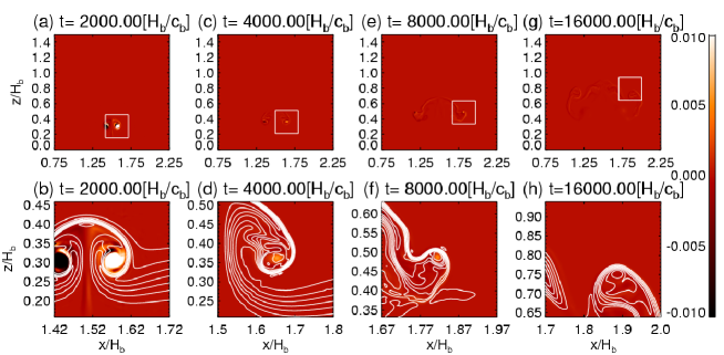
Figure 4: Temporal evolution of contours of vorticity normalized by $c_{\mathrm{b}}/H_{\mathrm{b}}$ in the case with a poloidal field. The white rectangles in panels a, c, e, and g indicate the region of the panels b, d, f, and h, respectively. The white lines in panels b, d, f, and h show the poloidal magnetic field line.

There are several possibilities for generating the twist. One is that the dynamo process itself is responsible for it. The second possibility is that the turbulent effect stemming from the rotation on the flux tube generates the twist, which is called the $\Sigma$-effect (Longcope et al., 1998). Another interesting explanation for the origin of the twist is given by Choudhuri (2003). In his explanation, the rising toroidal field is wrapped by a surrounding mean poloidal field and then gets twisted (see Fig. 4 of his 2003 paper). Choudhuri et al. (2004) report that, based on this idea and the Babcock-Leighton flux-transport dynamo model, the latitudinal dependence of twist can be reproduced during most of the duration of the solar cycle. Chatterjee et al. (2006) modeled the evolution of the rising magnetic flux tube with the accretion of the mean poloidal magnetic field by solving the induction equation. They report that without turbulent diffusivity the accreted poloidal flux is confined in a sheath at the outer periphery of the rising tube. Using plausible assumption and free parameters, they could obtain the value of $\alpha$ that is comparable to the observational result.

In this paper, we investigate the generation mechanism of twist based on the idea of Choudhuri (2003) in two-dimensional magnetohydrodynamics (MHD) calculations using the parameters at the base of the solar convection zone.

2 Model

We solve the compressive MHD equations in two-dimensional Cartesian geometry ($x,z$), where $x$ and $z$ denote the horizontal and vertical directions. The magnetic field has three components, i.e., ${\bf B}=(B_{x},B_{y},B_{z})$ even in two dimensions. Equations are expressed as

$$\frac{\partial\rho_{1}}{\partial t}=-\frac{1}{\xi^{2}}\nabla\cdot(\rho{\bf v}),$$ (1)

$$\frac{\partial}{\partial t}\left(\rho{\bf v}\right)=-\nabla\cdot\left[\rho{\bf vv}+\left(p_{1}+\frac{B^{2}}{8\pi}\right){\bf I}-\frac{\bf BB}{4\pi}\right]-\rho_{1}g{\bf e_{z}},$$ (2)

$$\frac{\partial{\bf B}}{\partial t}=\nabla\times({\bf v}\times{\bf B}),$$ (3)

$$\frac{\partial s_{1}}{\partial t}=-{\bf v}\cdot\nabla s,$$ (4)

$$p_{1}=p_{0}\left(\gamma\frac{\rho_{1}}{\rho_{0}}+\frac{s_{1}}{c_{\mathrm{v}}}\right)$$ (5)

where $\rho_{1}$, $p_{1}$, and $s_{1}$ denote the fluctuation of density, pressure, and the specific entropy. ${\bf v}$, ${\bf B}$, $g$, and $c_{\mathrm{v}}$ denote fluid velocity, magnetic field, gravitational acceleration, and the heat capacity at constant volume. The divergence-free condition, i.e. $\nabla\cdot{\bf B}=0$, is maintained numerically using the method introduced in Dedner et al. (2002). The medium is assumed to be an inviscid perfect gas with a specific heat ratio $\gamma=5/3$. The background values of density ($\rho_{0}$), pressure ($p_{0}$), and specific entropy ($s_{0}$) are assumed to be in an adiabatic stratification with constant gravitational acceleration as

$$p_{0}=p_{\mathrm{b}}\left[1-\nabla_{\mathrm{ad}}\frac{z}{H_{\mathrm{b}}}\right]^{1/\nabla_{\mathrm{ad}}},$$ (6)

$$\rho_{0}=\rho_{\mathrm{b}}\left[1-\nabla_{\mathrm{ad}}\frac{z}{H_{\mathrm{b}}}\right]^{1/\nabla_{\mathrm{ad}}-1},$$ (7)

$$s_{0}=c_{\mathrm{v}}\log\left(\frac{p_{0}}{\rho_{0}^{\gamma}}\right),$$ (8)

$$H_{\mathrm{b}}=\frac{p_{\mathrm{b}}}{\rho_{\mathrm{b}}g},$$ (9)

where $p_{\mathrm{b}}$, $\rho_{\mathrm{b}}$, and $H_{\mathrm{b}}$ are the background pressure, density, and pressure scale height at the bottom boundary. $\nabla_{\mathrm{ad}}=(\gamma-1)/\gamma$ denotes the adiabatic temperature gradient. We use the relation $\rho=\rho_{0}+\rho_{1}$, $p=p_{0}+p_{1}$, and $s=s_{0}+s_{1}$. The reduced speed of sound technique (hereafter RSST), which is introduced in Rempel (2005) and Hotta et al. (2012b), is used in this study, and $\xi$ denotes the ratio between the original and reduced speed of sound. The investigation of the validity of RSST for the flux rising is given in Hotta et al. (in preparation). In the initial condition, the toroidal magnetic flux tube ($B_{y}$) is set near the bottom boundary as

$$B_{y}=\left\{\begin{array}[]{ll}B_{\mathrm{t}}\exp\left(-{\displaystyle\frac{r^{2}}{d^{2}}}\right)&\mathrm{where}\ r<2d,\\ 0&\mathrm{where}\ r\geq 2d,\end{array}\right.$$ (12)

$$r^{2}=(x-x_{\mathrm{c}})^{2}+(z-z_{\mathrm{c}})^{2},$$ (13)

$$B_{\mathrm{t}}=\sqrt{\frac{8\pi p_{\mathrm{b}}}{\beta_{\mathrm{t}}+1}},$$ (14)

where $\beta_{\mathrm{t}}=1.6\times 10^{5}$ is the plasma beta of the toroidal field. $(x_{\mathrm{c}},z_{\mathrm{c}})=(1.5H_{\mathrm{b}},0.15H_{\mathrm{b}})$, and $d=0.03H_{\mathrm{b}}$ are the location and the radius of the flux tube. Two cases with or without poloidal magnetic flux sheet are given in §3. A poloidal magnetic flux sheet ($B_{x}$) is set above the toroidal field as

$$B_{x}=B_{\mathrm{p}}\exp\left[-\left(\frac{z-z_{\mathrm{p}}}{d_{\mathrm{p}}}\right)^{2}\right],$$ (15)

$$z_{\mathrm{p}}=z_{\mathrm{c}}+2d+d_{\mathrm{p}},$$ (16)

$$B_{\mathrm{p}}=\sqrt{\frac{8\pi p_{\mathrm{b}}}{\beta_{\mathrm{p}}+1}},$$ (17)

where $\beta_{\mathrm{p}}=10^{10}$ is the plasma beta for the poloidal field, and $z_{\mathrm{p}}$ and $d_{\mathrm{p}}=0.08H_{\mathrm{p}}$ are the location and thickness of the poloidal layer. The vertical magnetic field is set as $B_{z}=0$. Figures 1a and b show pictures of the initial condition, where the fluctuation of the pressure is set as $p_{1}=-B^{2}/(8\pi)$, and $s_{1}=0$. The radius and strength of the toroidal magnetic field is $d=1.8\times 10^{8}\ \mathrm{cm}$ and $B_{\mathrm{}}\sim 1\times 10^{5}\ \mathrm{G}$ if we adopt the parameters at the base of the solar convection zone; i.e., $H_{\mathrm{b}}=6\times 10^{9}\ \mathrm{cm}$, $\rho_{\mathrm{b}}=0.2\ \mathrm{g\ cm^{-3}}$, and the speed of sound at the bottom $c_{\mathrm{b}}=2.2\times 10^{7}\ \mathrm{cm\ s^{-1}}$. These values are plausible at the solar convection zone, since the “explosion” process can amplify the magnetic field up to $1\times 10^{5}\ \mathrm{G}$ at the base (Hotta et al., 2012a), and the magnetic field with this strength can reproduce the observational result of the tilt angle of sunspot pairs at the surface, i.e. Joy’s law, (Weber et al., 2011). Owing to a lack of information on the strength and the distribution of poloidal field from observation, we assumed the thickness and the strength of the poloidal magnetic field layer as $d=4.8\times 10^{8}\ \mathrm{cm}$ and $B_{\mathrm{p}}\sim 400\ \mathrm{G}$.

The simulation domain extends as $(0,0)<(x/H_{\mathrm{b}},z/H_{\mathrm{b}})<(3,1.5)$. The periodic boundary condition is used for all variables at $x=0,\ 3H_{\mathrm{b}}$. At the top and bottom boundaries, the stress-free and nonpenetrating boundary condition is adopted. A symmetric boundary condition for the magnetic field and density, i.e. $\partial B_{x}/\partial z=\partial B_{y}/\partial z=\partial B_{z}/\partial z=0$ and $\partial\rho_{1}/\partial z=0$, is used and entropy is fixed as $s_{1}=0$ at the top and bottom boundaries. The adaptive mesh refinement (hereafter AMR) technique is also used, since in this study the magnetic flux is highly localized. A self-similar block-structured grid is adopted as the grid of the AMR hierarchy (Matsumoto, 2007). In this study, the finest grid is equal to the grid using $1024\times 512$ in uniform structure. The fourth-order, space-centered difference and fourth-order Runge-Kutta for the time integration are used (Vögler et al., 2005). The details of our AMR code will be given in our forthcoming paper.

3 Result and discussion

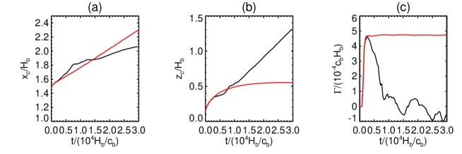
Figure 3: Temporal evolution of the center of the flux tube, (a) $x_{\mathrm{c}}$, (b) $z_{\mathrm{c}}$, and (c) the circulation $\Gamma$. The black (red) line denotes the result with (without) the poloidal magnetic field.

Figure 2 shows the result of the case without the mean poloidal field ($\beta_{\mathrm{p}}=\infty$) at $t=10^{4}H_{\mathrm{b}}/c_{\mathrm{b}}$. The magnetic flux tube quickly splits and ceases to rise. This result is almost the same as previous studies (Schüssler, 1979; Longcope et al., 1996). Figure 3 (red lines) shows the temporal evolution of the center of the splitted flux tube ($x_{\mathrm{c}},z_{\mathrm{c}}$) and the circulation $\Gamma$. We define the center of a splitted flux tube ($x_{\mathrm{c}},z_{\mathrm{c}}$) as the point where the magnetic field has maximum value in the region $x>1.5H_{\mathrm{b}}$. The circulation $\Gamma$ is defined as

$$\Gamma\equiv\int_{x_{\mathrm{c}}-d_{\mathrm{c}}}^{x_{\mathrm{c}}+d_{\mathrm{c}}}\int_{z_{\mathrm{c}}-d_{\mathrm{c}}}^{z_{\mathrm{c}}+d_{\mathrm{c}}}(\nabla\times{\bf v})_{y}dxdz,$$ (18)

where $d_{\mathrm{c}}=0.06H_{\mathrm{b}}$. The lifting force caused by circulation and horizontal motion ($F_{\mathrm{lif}}$) and the buoyancy ($F_{\mathrm{buo}}$) can be expressed as

$$F_{\mathrm{lif}}=-\rho V_{x}\Gamma,$$ (19)

$$F_{\mathrm{buo}}=-g\int_{x_{\mathrm{c}}-d_{\mathrm{c}}}^{x_{\mathrm{c}}+d_{\mathrm{c}}}\int_{z_{\mathrm{c}}-d_{\mathrm{c}}}^{z_{\mathrm{c}}+d_{\mathrm{c}}}\rho_{1}dxdz,$$ (20)

where $V_{x}$ is the bulk horizontal velocity of the flux tube. In the final stage, the lifting force (directed downward) and the buoyancy (directed upward) are almost balanced in the vertical direction. Since the flux tube rises vertically in the first stage, it is accelerated horizontally by the horizontal lifting force $\rho V_{z}\Gamma$, where $V_{z}$ is the vertical bulk velocity of the flux tube. By this driven horizontal motion, a downward lifting force is induced and must be balanced with the buoyancy force at a certain point.

Figures 2c and d show the distribution of angular velocity and angular momentum. We define the center of the rotating motion at the point where vorticity has maximum value (see the asterisk in Fig 2b). The result shows that the angular velocity increases radially, while the angular momentum decreases. We discuss the consequence of such distribution in §4.

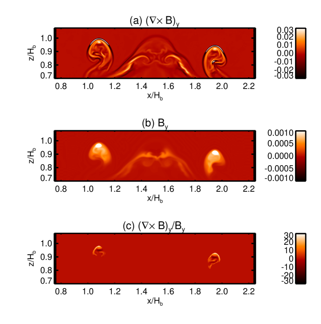
Figure 5: Values in $t=20000H_{\mathrm{b}}/c_{\mathrm{b}}$. (a) The contour of $(\nabla\times{\bf B})_{y}$ normalized with $B_{0}/H_{\mathrm{b}}$. Positive value shows the clockwise poloidal fields. (b) The contour of Toroidal field $B_{y}$ normalized by $B_{0}$. (c) The contour of $(\nabla\times{\bf B})_{y}/B_{y}$ normalized by $H_{\mathrm{b}}^{-1}$. The value is only calculated in the place where the strength of toroidal field exceeds $6\times 10^{-4}B_{0}$.

Figures 1 and 4 show the result of the case with the mean poloidal field ($\beta_{\mathrm{p}}=10^{10}$) . In the first stage, similar to the case without the poloidal field, the flux tube splits and moves horizontally with large vorticity (Figs. 4a and b). Then this vorticity gradually decreases (Figs. 4c, d, e, and f). When the flux tube loses almost all circulation the magnetic flux begins to rise again (Figs. 1g, and h, 4g, and h). Figure 3 (black line) also shows these processes, i.e., re-arisal occurs when circulation decreases around $t=5000H_{\mathrm{b}}/c_{\mathrm{b}}$. Figure 1h shows that after this process the magnetic flux gets twisted. Although it is not shown, these twisted magnetic flux tubes rise to the upper boundary without splitting in the final stage of this simulation. We note that, although the flux tubes have vortices of different signs, the signs of the generated twist on two flux tubes are the same since the directions of the poloidal field and the toroidal field are the same between two tubes. Figure 5a, b, and c show the values of $(\nabla\times B)_{y}$, $B_{y}$, and $(\nabla\times B)_{y}/B_{y}$, respectively. The global structure of the poloidal field is shown clockwise, and the average of the values of the twist is positive near the core of the toroidal field in both flux tubes.

We investigated the detailed process of the losing of circulation in the the case with the initial poloidal layer. Figure 6 shows the temporal evolution of the magnetic tension perpendicular to the magnetic field line ($T_{\perp}$), i.e,

$$T_{\perp}={\bf e}_{\perp}\cdot\left[\left({\bf B}\cdot\nabla\right){\bf B}\right],$$ (21)

where ${\bf e}_{\perp}={\bf B}\times{\bf\omega}/(|{\bf B}||{\bf\omega}|)$ is the unit vector perpendicular to the magnetic field and the vorticity and ${\bf\omega}=\nabla\times{\bf v}$. The poloidal field lines are suddenly bent (see in Fig. 6). This type of sudden bending event on the magnetic field lines occurs frequently at the point where the poloidal magnetic energy is less than the energy of rotation. Since the magnetic field is stretched and amplified during this process, the feedback by the magnetic tension efficiently suppresses circulating motion. This can be seen in Fig. 6. The high positive value of the magnetic tension indicates the feedback effect. We recall that when the mean poloidal field does not exist, the angular velocity increases and the angular momentum decreases radially (Fig. 2). This configuration is similar to that of the magneto-rotational instability (Chandrasekhar, 1960): the rolled-up poloidal magnetic field can be bent up to the interior of the flux tube. When the poloidal magnetic field has finite disturbance, the inner part that is rotating faster loses the angular momentum due to the magnetic tension, i.e., the interaction with the outer slow-rotating part. In this case, the medium that loses angular momentum moves inward radially, and the bending of the poloidal magnetic field increases. Therefore the flux tube obtains the twist, which distributes it over the tube’s cross section without a localization in the boundary layer. We have determined that when the magnetic field is bent, the structure of circulation is similar to that of the first case without the poloidal field; i.e., the angular velocity increases and the angular momentum decreases.

Our results seem to suggest that two flux tubes may emerge and form active regions in different latitudes simultaneously. This probably does not occur because of the modulation of the tube’s emerging motion by the thermal convection. Weber et al. (2011) have studied the rising of the magnetic flux through the solar convection zone by using the thin-flux-tube approximation with the effect of thermal convection and find that the timing of emergence differs by more than one month between tubes from different latitudes (see their Fig. 8) and that the emerging latitude is also scattered typically over ten degrees (see their Fig. 11) with the strength of a magnetic field of $4\times 10^{4}$ G, which is the strength of our splitted magnetic flux on their re-rising. Their results suggest that our split pair tubes also emerge with these spatial and temporal scattering offsets. Our splitted flux tubes separated about $1H_{\mathrm{p}}$, which corresponds to five degrees in latitude and well below the predicted scatter (10 degrees, Weber et al., 2011)

4 Summary

Using two-dimensional magnetohydrodynamics calculations, we investigated a twist-generation mechanism on a magnetic flux tube at the base of the solar convection zone. It is based on the idea of Choudhuri (2003) in which a toroidal magnetic field is wrapped by a surrounding mean poloidal field. During the generation of the twist, the flux tube follows four phases. (1) The flux tube quickly splits into two parts with vortex motions rolling up the poloidal magnetic field. (2) Because the physical mechanism is similar to that of the magneto-rotational instability, the rolled-up poloidal field is bent and amplified. (3) The magnetic tension of the disturbed poloidal magnetic field reduces the vorticity, and the lifting force caused by vortical motion decreases. (4) The flux tube gets twisted and begins to rise again without splitting.

With the use of the reduced RSST (Hotta et al., 2012b) and AMR, it became possible to adopt parameters that are acceptable at the base of the solar convection zone, i.e., the radius of flux tube $d=1.8\times 10^{8}\ \mathrm{cm}$ and the strength of the toroidal field $B\sim 1\times 10^{5}\ \mathrm{G}$. In this study, we use $400\ \mathrm{G}$ as the strength of the poloidal field. It is expected that a certain level of strength of such a poloidal field is necessary for suppressing the circulation motion and the ensuing flux tube’s rising again. The criterion for rising again is an interesting issue. The detailed parameter survey will be given in our forthcoming paper.

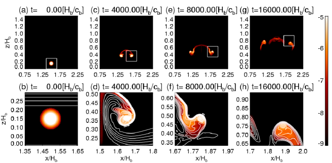
Figure 1: Temporal evolution of contours of toroidal magnetic field ($\log[(B_{y}/B_{0})^{2}]$) in cases with a poloidal magnetic field, where $B_{0}^{2}/(8\pi)=\rho_{\mathrm{b}}c_{\mathrm{b}}^{2}$. The white rectangles in panels a, c, e, and g indicate the region of the panels b, d, f, and h, respectively. The white lines in panels b, d, f, and h show the poloidal magnetic field lines.

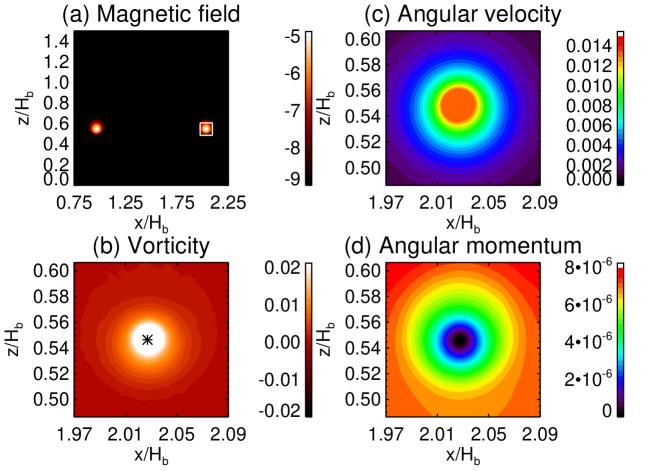
Figure 2: The results without poloidal field at $t=10^{4}H_{\mathrm{b}}/c_{\mathrm{b}}$. (a) The contour of toroidal magnetic field ($\log[(B_{y}/B_{0})^{2}]$). (b) The vorticity of $y$-direction in the white rectangle in panel a normalized by $c_{\mathrm{b}}/H_{\mathrm{b}}$. The point where vorticity has a maximum value is indicated with an asterisk. This point is defined as the origin of a circular geometry in order to calculate angular velocity and angular momentum. (c) The angular velocity normalized by $c_{\mathrm{b}}/H_{\mathrm{b}}$. (d) The angular momentum normalized by $\rho_{\mathrm{b}}H_{\mathrm{b}}c_{\mathrm{b}}$.

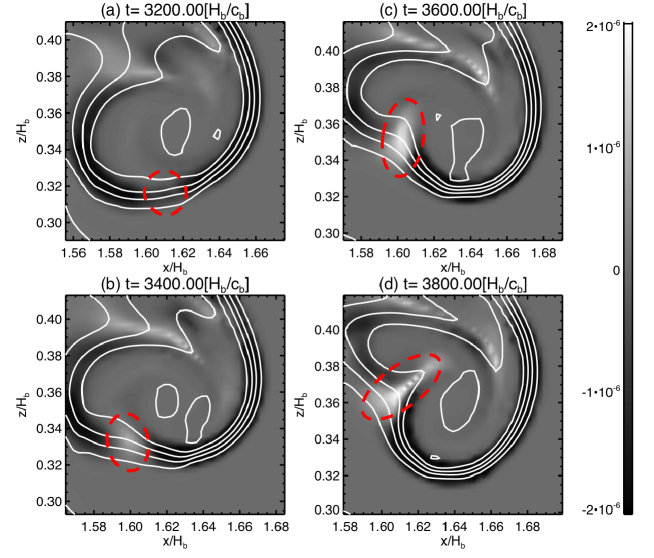
Figure 6: Temporal evolution of magnetic tension ($T_{\perp}$: Eq. 21) normalized by $B_{0}^{2}/H_{\mathrm{b}}$ in the case with a poloidal field. Red circles indicate the location of the bending event.

References

- Chandrasekhar (1960) Chandrasekhar, S. 1960, Proceedings of the National Academy of Science, 46, 253
- Chatterjee et al. (2006) Chatterjee, P., Choudhuri, A. R., & Petrovay, K. 2006, A&A, 449, 781
- Choudhuri (2003) Choudhuri, A. R. 2003, Sol. Phys., 215, 31
- Choudhuri et al. (2004) Choudhuri, A. R., Chatterjee, P., & Nandy, D. 2004, ApJ, 615, L57
- Choudhuri et al. (1995) Choudhuri, A. R., Schüssler, M., & Dikpati, M. 1995, A&A, 303, L29
- Dedner et al. (2002) Dedner, A., Kemm, F., Kröner, D., et al. 2002, Journal of Computational Physics, 175, 645
- Dikpati & Charbonneau (1999) Dikpati, M. & Charbonneau, P. 1999, ApJ, 518, 508
- Fan (2009) Fan, Y. 2009, Living Reviews in Solar Physics, 6, 4
- Hotta et al. (2012a) Hotta, H., Rempel, M., & Yokoyama, T. 2012a, ApJ, 759, L24
- Hotta et al. (2012b) Hotta, H., Rempel, M., Yokoyama, T., Iida, Y., & Fan, Y. 2012b, A&A, 539, A30
- Hotta & Yokoyama (2010a) Hotta, H. & Yokoyama, T. 2010a, ApJ, 709, 1009
- Hotta & Yokoyama (2010b) Hotta, H. & Yokoyama, T. 2010b, ApJ, 714, L308
- Longcope et al. (1996) Longcope, D. W., Fisher, G. H., & Arendt, S. 1996, ApJ, 464, 999
- Longcope et al. (1998) Longcope, D. W., Fisher, G. H., & Pevtsov, A. A. 1998, ApJ, 507, 417
- Matsumoto (2007) Matsumoto, T. 2007, PASJ, 59, 905
- Moreno-Insertis & Emonet (1996) Moreno-Insertis, F. & Emonet, T. 1996, ApJ, 472, L53
- Parker (1955) Parker, E. N. 1955, ApJ, 122, 293
- Pevtsov et al. (2001) Pevtsov, A. A., Canfield, R. C., & Latushko, S. M. 2001, ApJ, 549, L261
- Pevtsov et al. (1995) Pevtsov, A. A., Canfield, R. C., & Metcalf, T. R. 1995, ApJ, 440, L109
- Pevtsov et al. (2003) Pevtsov, A. A., Maleev, V. M., & Longcope, D. W. 2003, ApJ, 593, 1217
- Rempel (2005) Rempel, M. 2005, ApJ, 622, 1320
- Schüssler (1979) Schüssler, M. 1979, A&A, 71, 79
- Vögler et al. (2005) Vögler, A., Shelyag, S., Schüssler, M., et al. 2005, A&A, 429, 335
- Weber et al. (2011) Weber, M. A., Fan, Y., & Miesch, M. S. 2011, ApJ, 741, 11