Depth properties of Scaled Attachment Random Recursive Trees

Abstract.

We study depth properties of a general class of random recursive trees where each node $i$ attaches to the random node $\left\lfloor iX_{i}\right\rfloor$ and $X_{0},\dots,X_{n}$ is a sequence of i.i.d. random variables taking values in $[0,1)$. We call such trees scaled attachment random recursive trees (sarrt). We prove that the typical depth $D_{n}$, the maximum depth (or height) $H_{n}$ and the minimum depth $M_{n}$ of a sarrt are asymptotically given by $D_{n}\sim\mu^{-1}\log n$, $H_{n}\sim\alpha_{\max}\log n$ and $M_{n}\sim\alpha_{\min}\log n$ where $\mu,\alpha_{\max}$ and $\alpha_{\min}$ are constants depending only on the distribution of $X_{0}$ whenever $X_{0}$ has a density. In particular, this gives a new elementary proof for the height of uniform random recursive trees $H_{n}\sim e\log n$ that does not use branching random walks.

1. Introduction

A uniform random recursive tree (urrt) $T_{n}$ of order $n$ is a tree with $n+1$ nodes labeled $\{0,1,\dots,n\}$ constructed as follows. The root is labeled $0$, and for $1\leq i\leq n$, the node labeled $i$ is inserted and chooses a vertex in $\{0,\dots,i-1\}$ uniformly at random as its parent. The asymptotic properties of $T_{n}$ – the depth of the last inserted node, the height of the tree, the degree distribution, the number of leaves, the profile and so forth – have been extensively studied starting from Moon [23], Gastwirth [18] and Na and Rapoport [24]. In particular, Szymański [31] showed that the depth $D_{n}$ of node $n$ is $(1+o(1))\log n$ with probability going to $1$ and Pittel [26] proved that the height $H_{n}$ is $(e+o(1))\log n$ with probability going to $1$. Distance measures in a urrt were also considered by Dobrow [13], Dobrow and Fill [14], Meir and Moon [22], Neininger [25] and Su et al. [29]. For a survey, see Drmota [15] and Smythe and Mahmoud [28].

A natural generalization of this model introduced by Devroye and Lu [11] is to let a vertex choose $k>1$ parents uniformly. This construction defines a random directed acyclic graph ($k$-dag), which was used to model circuits Tsukiji and Xhafa [32], Arya et al. [2].

The uniformity condition was relaxed by Szymański [30] by letting the probabilities of being chosen as a parent depend on the degree of the parent. When the probability of linking to a node is proportional to its degree, this gives a random plane-oriented recursive tree, the typical depth of which was studied by Mahmoud [20] and the height of which was studied by Pittel [26]. When $k>1$ parents are chosen for each node, the popular preferential attachment model of Barabasi and Albert [3] is obtained.

Motivated by recent work on distances in random $k$-dags (Devroye and Janson [10]) and on the power of choice in the construction of random trees (D’Souza et al. [16], Mahmoud [21]), we introduce a generalization of uniform random recursive trees. In a scaled attachment random recursive tree (sarrt), a node $i$ chooses its parent to be the node labeled $\left\lfloor iX_{i}\right\rfloor$ where $X_{0},X_{1},\dots,X_{n}$ is a sequence of independent random variables distributed as $X$ over $[0,1)$. Note that the choice of the parent here only depends on the labels of previous nodes and not on their properties relative to the tree (like the degree, for example). In particular, if $X$ is uniform on $[0,1)$ we get a urrt. The distribution $\mathcal{L}(X)$ of $X$ is called the attachment distribution.

We study properties of the depth (path distance to the root of the tree) of nodes in a sarrt with a general attachment distribution. We determine the first-order asymptotics for the depth $D_{n}$ of the node labeled $n$, the height $H_{n}=\max_{1\leq i\leq n}D_{i}$ of the tree and the minimum depth $M_{n}=\min_{n/2\leq i\leq n}D_{i}$. Our result gives a new way of computing the height of a urrt that is not based on branching random walks that were used in previous proofs by Devroye [9] and Pittel [26].

Furthermore, setting $X=\max(U_{1},\dots,U_{k})$ where $U_{1},\dots,U_{k}$ are independent random variables with uniform distribution over $[0,1)$, the depth $D_{i}$ of node $i$ in a sarrt with attachment $X$ is the distance given by following the oldest parent from node $i$ to the root in a random $k$-dag [10, 21]. This problem can be seen as a “power of choice” question: how much can one optimize properties of the tree when each node is given $k$ choices of parents? A new node is given $k$ choices of parents, and it selects the best one according to some criterion. In the setting of this paper, we study selection criteria that only depend on the labels or arrival times of the potential parents. Our results describe the influence of a large class of such selection criteria on the depth of the last inserted node, the height and the minimum depth of the tree. This holds for a urrt and for almost any sarrt as well. Some examples are given in Section 5.

Outline of the results. In Section 2, we prove a concentration result and a central limit theorem for $D_{n}$ for a very general class of attachment distributions:

$$\frac{D_{n}}{\log n}\overset{\mathcal{P}}{\to}\frac{1}{\mu}\qquad\text{and}\qquad\frac{D_{n}-\mu^{-1}\log n}{\sigma\sqrt{\mu^{-3}\log n}}\overset{\mathcal{L}}{\to}\mathcal{N}(0,1),$$

where $\mu$ and $\sigma^{2}$ are simply the expected value and the variance of $-\log X$, $\mathcal{N}(0,1)$ denotes the standard Gaussian distribution and the symbols $\overset{\mathcal{P}}{\to}$ and $\overset{\mathcal{L}}{\to}$ refer to convergence in probability and convergence in distribution. This generalizes a result of Mahmoud [21]. In Sections 3 and 4, we prove the main theorems (Theorems 2 and 6) of this paper: if $\mathcal{L}(X)$ has a density on $[0,1)$, then there exist constants $\alpha_{\max}$ and $\alpha_{\min}$ such that

$$\lim_{n\to\infty}\frac{H_{n}}{\log n}=\alpha_{\max}\quad\text{almost surely},\qquad\text{and}\qquad\frac{M_{n}}{\log n}\overset{\mathcal{P}}{\to}\alpha_{\min},$$

where $H_{n}$ and $M_{n}$ denote the height and minimum depth of the sarrt with attachment $X$. These constants are defined as the solutions of equations involving a rate function associated with $\log X$. The proof of these results uses a second moment method. The main difficulty in the proof is in controlling the dependencies between the paths up to the root that originate from different nodes. We also prove that $\lim_{n\to\infty}\frac{\mathbf{E}\left\{H_{n}\right\}}{\log n}=\alpha_{\max}$.

The different results are applied to study the properties of various path lengths in a random $k$-dag in Section 5. Lastly, we include an appendix proving some simple properties of the large deviation rate functions used.

Notation. As introduced earlier, the symbols $\overset{\mathcal{P}}{\to}$ and $\overset{\mathcal{L}}{\to}$ refer to convergence in probability and convergence in distribution respectively. For random variables $X$ and $Y$, we write $\mathcal{L}(X)$ for the distribution of $X$ and $X\stackrel{{\scriptstyle\mathcal{L}}}{{=}}Y$ when $X$ and $Y$ have the same distribution. For a general random variable $X\in[0,1)$, we define

$$\mu=\mathbf{E}\left\{-\log X\right\}\geq 0\qquad\text{and}\qquad\sigma^{2}=\mathbf{Var}\left\{-\log X\right\}.$$

If $X$ has an atom at $0$, then $\mu=\sigma=+\infty$. If $\mu=+\infty$, then we define $\sigma=+\infty$. A sarrt with attachment distribution $\mathcal{L}(X)$ is described by a sequence $X_{0},X_{1},\dots,X_{n}$ of i.i.d. random variables distributed as $X$. The parent of node $i$ is labeled $\left\lfloor iX_{i}\right\rfloor$. The root of the tree is labeled $0$ and $L(n,j)$ is the (random) label of the $j$-th grandparent of $n$ on its path to the root. Note that $L(n,j+1)=\left\lfloor L(n,j)X_{L(n,j)}\right\rfloor$ and that $L(n,0)=n$. The depth $D_{i}$ of node $i$ is defined by $D_{i}=\min\{j\geq 0:L(i,j)=0\}.$

2. The depth of a typical node

We look at the sequence of labels from node $n$ to the root as a renewal process. We have

$$D_{n} =\min\{j\geq 0:L(n,j)=0\}$$

$$=\min\{j\geq 0:\left\lfloor\dots\left\lfloor\left\lfloor nX_{n}\right\rfloor X_{L(n,1)}\right\rfloor\dots X_{L(n,j-1)}\right\rfloor=0\}.$$

Note that

$$nX_{n}X_{L(n,1)}\dots X_{L(n,j-1)}-j\leq\left\lfloor\dots\left\lfloor\left\lfloor nX_{n}\right\rfloor X_{L(n,1)}\right\rfloor\dots X_{L(n,j-1)}\right\rfloor\leq nX_{n}X_{L(n,1)}\dots X_{L(n,j-1)}.$$

Remark.

Since $X\in[0,1)$, we have $\mu=\mathbf{E}\left\{-\log X\right\}>0$. Thus, the following theorem covers all the possible cases.

Theorem 1.

(A) $$\text{If $\mu=+\infty$, then}\quad\frac{D_{n}}{\log n}\overset{\mathcal{P}}{\to}0\quad\text{ and }\quad\lim_{n\to\infty}\frac{\mathbf{E}\left\{D_{n}\right\}}{\log n}=0.$$

(B) $$\text{If $\mu<+\infty$, then}\quad\frac{D_{n}}{\log n}\overset{\mathcal{P}}{\to}\frac{1}{\mu}\quad\text{ and }\quad\lim_{n\to\infty}\frac{\mathbf{E}\left\{D_{n}\right\}}{\log n}=\frac{1}{\mu}.$$

(C) $$\text{If $\mu<+\infty$ and $0<\sigma^{2}<+\infty$, then}\quad\frac{D_{n}-\log n/\mu}{\sigma\sqrt{\log n/\mu^{3}}}\overset{\mathcal{L}}{\to}\mathcal{N}(0,1).$$

(D) $$\text{If $\mu<+\infty$ and $\sigma^{2}=0$, then}\quad D_{n}-\log n/\mu=o\left(\sqrt{\log n}\right)\quad\text{almost surely.}$$

Remark.

Mahmoud [21] proved a similar result using generating functions for the case $X\stackrel{{\scriptstyle\mathcal{L}}}{{=}}\max(U_{1},\dots,U_{k})$ and $X\stackrel{{\scriptstyle\mathcal{L}}}{{=}}\min(U_{1},\dots,U_{k})$. Details are given in Section 5.

Proof.

We consider an auxiliary renewal process $R_{t}=\sup\big{\{}j:\sum_{i=1}^{j}Z_{i}\leq t\big{\}}$ with interarrival times distributed as $Z_{i}\stackrel{{\scriptstyle\mathcal{L}}}{{=}}-\log X$ for all $i$. When $\mu<+\infty$, the strong law of large numbers for renewal processes gives that $R_{t}/t\to 1/\mu$ almost surely (see 27, Proposition 3.3.1). Moreover, the elementary renewal theorem implies that $\mathbf{E}\left\{R_{t}\right\}/t\to 1/\mu$. The following claim handles the case $\mu=+\infty$.

Claim.

For $\mu=+\infty$, $\lim_{t\to\infty}\frac{R_{t}}{t}=0$ with probability $1$ and $\lim_{t\to\infty}\frac{\mathbf{E}\left\{R_{t}\right\}}{t}=0$.

Proof.

For fixed $b>0$, let $\widetilde{Z}_{i}=\min(Z_{i},a)$ where $a$ is chosen so that $\mathbf{E}\big{\{}\widetilde{Z}_{i}\big{\}}\geq b$. Consider the renewal process $\widetilde{R}_{t}$ with interarrival times $\widetilde{Z}_{i}$. By the fact that $R_{t}\leq\widetilde{R}_{t}$ and the law of large numbers for $\widetilde{R}_{t}$ we have, for sufficiently large $t$, $R_{t}/t\leq\widetilde{R}_{t}/t<2/b$ almost surely. Since $b$ is arbitrary, we have $R_{t}/t\to 0$ with probability 1. The convergence of the expected value is proved in a similar way. This concludes the proof of the claim. ∎

We upper bound the depth of node $n$ by

$$D_{n} \leq\min\left\{j:nX_{n}X_{L(n,1)}\dots X_{L(n,j-1)}<1\right\}$$

$$=\min\left\{j:\textstyle{\sum}_{i=0}^{j-1}-\log X_{L(n,i)}>\log n\right\}\stackrel{{\scriptstyle\textrm{def}}}{{=}}\widehat{D}_{n}.$$

For $n\geq 1$, $\widehat{D}_{n}\stackrel{{\scriptstyle\mathcal{L}}}{{=}}R_{\log n}+1$. So, we have for any $\varepsilon>0$ that

(1) $$\mathbf{P}\left\{\frac{D_{n}}{\log n}>\frac{1}{\mu}+\varepsilon\right\}\leq\mathbf{P}\left\{\frac{\widehat{D}_{n}}{\log n}>\frac{1}{\mu}+\varepsilon\right\}=\mathbf{P}\left\{\frac{R_{\log n}+1}{\log n}>\frac{1}{\mu}+\varepsilon\right\}=o(1).$$

Since $D_{n}>0$, equation (1) proves part (A) of the theorem (by writing $1/\mu=0$ when $\mu=+\infty$).

Similarly, a lower bound is given by

$$D_{n} \geq\min\left\{j:nX_{n}\dots X_{L(n,j-1)}-j<1\right\}$$

$$\geq\min\left\{j:\textstyle{\sum}_{i=0}^{j-1}-\log X_{L(n,i)}>\log n-\log j\right\}.$$

Let $j(n)=\left\lfloor\log^{2}n\right\rfloor$ and define the event

$$E_{n}=\left[\;\sum_{i=0}^{j(n)-1}-\log X_{L(n,i)}>\log n\,\right].$$

Using the upper bound (1), we have that $\mathbf{P}\left\{E_{n}\right\}\to 1$. Also, we have $\log j\leq 2\log\log n$ and if we define $f(n)=\log n-2\log\log n$, then when $E_{n}$ holds

$$D_{n} \geq\min\left\{j:\textstyle{\sum}_{i=0}^{j-1}-\log X_{L(n,i)}>f(n)\right\}\stackrel{{\scriptstyle\textrm{def}}}{{=}}\overline{D}_{n}.$$

We have $\overline{D}_{n}\stackrel{{\scriptstyle\mathcal{L}}}{{=}}R_{f(n)}+1$ for $n\geq 2$, and thus,

(2) $$\mathbf{P}\left\{\frac{\overline{D}_{n}}{\log n}<\frac{1}{\mu}-\varepsilon\right\}=\mathbf{P}\left\{\frac{R_{f(n)}+1}{f(n)}\cdot\frac{f(n)}{\log n}<\frac{1}{\mu}-\varepsilon\right\}=o(1),$$

by the law of large numbers for renewal processes and the fact that

$$\lim_{n\to\infty}\,\frac{f(n)}{\log n}=1.$$

Combining (1) and (2) with the fact that $\mathbf{P}\left\{D_{n}\geq\overline{D}_{n}\right\}\geq\mathbf{P}\left\{E_{n}\right\}$ we obtain convergence in probability of part (B) of the theorem. As for the expected value, we have for any $\varepsilon>0$,

$$(1/\mu-\varepsilon)\log n\cdot\mathbf{P}\left\{D_{n}\geq(1/\mu-\varepsilon)\log n\right\}\leq\mathbf{E}\left\{D_{n}\right\}\leq\mathbf{E}\left\{\widehat{D}_{n}\right\}$$

which completes the proof of (B).

By similar arguments using the central limit theorem for renewal processes (see 27, Theorem 3.3.5) we can prove part (C) for $D_{n}$, by showing that

$$\lim_{n\to\infty}\mathbf{P}\left\{\frac{\widehat{D}_{n}-\log n/\mu}{\sigma\sqrt{\log n/\mu^{3}}}\leq c\right\}=\Phi(c)\qquad\text{and}\qquad\lim_{n\to\infty}\mathbf{P}\left\{\frac{\overline{D}_{n}-\log n/\mu}{\sigma\sqrt{\log n/\mu^{3}}}\leq c\right\}=\Phi(c),$$

where $\Phi$ is the cumulative distribution function of a standard $\mathcal{N}(0,1)$ variable. The result follows from the fact that $\overline{D}_{n}\leq D_{n}\leq\widehat{D}_{n}$ with probability going to $1$ as $n\to\infty$. The first limit is clear and to show the second limit, write

$$\frac{\overline{D}_{n}-\log n/\mu}{\sigma\sqrt{\log n/\mu^{3}}}=\frac{\big{(}\overline{D}_{n}-f(n)/\mu\big{)}+\big{(}f(n)/\mu-\log n/\mu\big{)}}{\sigma\sqrt{f(n)/\mu^{3}}}\cdot\sqrt{\frac{f(n)}{\log n}}$$

where we have

$$\lim_{n\to\infty}\frac{f(n)/\mu-\log n/\mu}{\sigma\sqrt{f(n)/\mu^{3}}}=\lim_{n\to\infty}\frac{-2\log\log n/\mu}{\sigma\sqrt{f(n)/\mu^{3}}}=\lim_{n\to\infty}\frac{-2\log\log n/\mu}{\sigma\sqrt{\log n-2\log\log n/\mu^{3}}}=0.$$

Also, the central limit theorem for renewal processes implies that

$$\lim_{n\to\infty}\mathbf{P}\left\{\frac{\overline{D}_{n}-f(n)/\mu}{\sigma\sqrt{f(n)/\mu^{3}}}\leq c\right\}=\Phi(c).$$

When $\sigma^{2}=0$, $X=e^{-\mu}\in(0,1)$ almost surely. Then the label of node $i$ parent is $\left\lfloor ie^{-\mu}\right\rfloor$ and $L(n,j)=\left\lfloor\left\lfloor\left\lfloor ne^{-\mu}\right\rfloor e^{-\mu}\right\rfloor\dots e^{-\mu}\right\rfloor$ ($j$ times) almost surely. Since $ne^{-j\mu}-j\leq L(n,j)\leq ne^{-j\mu}$ and for $n\geq n_{0}(\mu)$ we have $ne^{-j\mu}<1$ when $j>\log n/\mu$ and $ne^{-j\mu}-j>1$ when $j<\log n/\mu$. Then, we have that $|D_{n}-\log n/\mu|\leq 1$ for $n\geq n_{0}$. Therefore we get part (D) of the theorem. ∎

3. The height of the tree

We turn our attention to the height $H_{n}=\max_{1\leq i\leq n}D_{i}$ of a sarrt. For a random variable $Y$, we define its cumulant generating function $\Lambda_{Y}$ and its convex (Fenchel–Legendre) dual $\Lambda^{*}_{Y}$ as follows:

(3) $$\Lambda_{Y}(\lambda)=\log\mathbf{E}\left\{e^{\lambda Y}\right\}\quad\text{and}\quad\Lambda^{*}_{Y}(z)=\sup_{\lambda\in\mathbb{R}}\big{\{}\lambda z-\Lambda_{Y}(\lambda)\big{\}}.$$

Since we mostly use these functions for $Y=\log X$, we omit the subscript in this case. We write

(4) $$\Lambda(\lambda)=\log\mathbf{E}\left\{e^{\lambda\log X}\right\}=\log\mathbf{E}\left\{X^{\lambda}\right\}\quad\text{and}\quad\Lambda^{*}(z)=\sup_{\lambda\in\mathbb{R}}\big{\{}\lambda z-\Lambda(\lambda)\big{\}}$$

for the cumulant generating function of $\log X$ and its dual. It is well known that $\Lambda^{*}(z)=\sup_{\lambda\geq 0}\big{\{}\lambda z-\Lambda(\lambda)\big{\}}$ for $z\geq\mathbf{E}\left\{\log X\right\}$ and $\Lambda^{*}(z)=\sup_{\lambda\leq 0}\big{\{}\lambda z-\Lambda(\lambda)\big{\}}$ for $z\leq\mathbf{E}\left\{\log X\right\}$. This is proved along with many properties of $\Lambda^{*}$ used in the paper in Appendix B. We also define

(5) $$\Psi(c)=c\Lambda^{*}\left(-1/c\right)$$

and

(6) $$\alpha_{\max}=\inf\left\{c:\;c>\frac{1}{\mu}\;\text{ and }\;\Psi(c)>1\right\}$$

where we define $1/\mu=0$ when $\mu=+\infty$. Proposition 5 in the appendix shows that the set $\left\{c:\;c>\frac{1}{\mu}\;\text{ and }\;\Psi(c)>1\right\}$ is non-empty, $\alpha_{\max}<+\infty$ and if $X$ is not a constant, $\alpha_{\max}>1/\mu$.

The following theorem sums up the results we prove in this section.

Theorem 2.

The height $H_{n}$ of a sarrt with attachment $X$ having a density satisfies

$$\lim_{n\to\infty}\frac{H_{n}}{\log n}=\alpha_{\max}\quad\text{with probability }1,\qquad\text{and}\qquad\lim_{n\to\infty}\frac{\mathbf{E}\left\{H_{n}\right\}}{\log n}=\alpha_{\max},$$

where $\alpha_{\max}$ is defined in equation (6).

Remark.

It is worth observing that if $X$ is not constant and $\mu=+\infty$, then $D_{n}=o(\log n)$ in probability as shown in Theorem 1, whereas $H_{n}=\Theta(\log n)$ in probability. If $X=\alpha\in(0,1)$ with probability $1$, then $\alpha_{\max}=1/\mu=-1/\log\alpha$ and it is easy to see that the results of the theorem also hold in this case.

We start by proving convergence in probability of $\frac{H_{n}}{\log n}$ in Sections 3.1 and 3.2 in the case of a bounded density. Section 3.1 gives an upper bound for $\frac{H_{n}}{\log n}$ with no condition on $X$. The lower bound we present in Section 3.2 is more involved and uses an upper bound on the density in order to bound the dependence between different paths. In Section 3.3, we show that the lower bound still holds if $X$ has an unbounded density. Finally, Section 3.4 is devoted to proving almost sure convergence and convergence in mean as stated in the above theorem.

3.1. The height of the tree: upper bound

Based on the bounding techniques of Chernoff [4] and Hoeffding [19] we can prove the following result.

Lemma 1.

For any $c>\alpha_{\max}$, we have $\mathbf{P}\left\{H_{n}\geq c\log n\right\}\to 0.$

Proof.

To simplify the notation, we prove $\mathbf{P}\left\{H_{n}\geq c\log n+2\right\}\to 0$ for all $c>\alpha_{\max}$, which is an equivalent statement. For $t\geq 1$, applying Markov’s inequality, we get

$$\mathbf{P}\left\{D_{n}>t\right\} \leq\mathbf{P}\left\{nX_{n}\dots X_{L(n,t-1)}\geq 1\right\}$$

$$\leq\inf_{\lambda\geq 0}n^{\lambda}\mathbf{E}\left\{X_{n}^{\lambda}\dots X_{L(n,t-1)}^{\lambda}\right\}$$

$$=\inf_{\lambda\geq 0}n^{\lambda}\mathbf{E}\left\{X^{\lambda}\right\}^{t}$$

$$=\inf_{\lambda\geq 0}\operatorname{exp}\left(\lambda\log n+\Lambda(\lambda)t\Big{.}\right)$$

Setting $t=\left\lceil c\log n\right\rceil$, we obtain

$$\mathbf{P}\left\{D_{n}\geq c\log n+2\right\} \leq\inf_{\lambda\geq 0}\operatorname{exp}\left(\lambda\log n+\Lambda(\lambda)c\log n\Big{.}\right), \Lambda(\lambda)\leq 0$$ (as )

$$\leq\operatorname{exp}\left(-\sup_{\lambda\geq 0}\left\{-\frac{\lambda}{c}-\Lambda(\lambda)\right\}c\log n\right)$$

$$=\operatorname{exp}\left(-c\Lambda^{*}\left(-1/c\right)\log n\right)$$

(7) $$=n^{-\Psi(c)}.$$

When $\Psi(c)>0$, the bound in (3.1) goes to $0$. Recalling that $c>\alpha_{\max}$ and the definition of $\alpha_{\max}$ (equation (6)), we obtain $\Psi(c)>1$. Applying a union bound, we get

(8) $$\mathbf{P}\left\{H_{n}>t\right\}=\mathbf{P}\left\{\max_{1\leq i\leq n}D_{i}>t\right\} \leq\sum_{i=1}^{n}\mathbf{P}\left\{D_{i}>t\right\}$$

$$\leq n\mathbf{P}\left\{D_{n}>t\right\}$$

$$\leq n^{1-\Psi(c)}\to 0$$

as $n\to\infty$. Note that the last inequality holds because $\left\lfloor\dots\left\lfloor\left\lfloor iX_{i}\right\rfloor X_{L(i,1)}\right\rfloor\dots X_{L(i,t-1)}\right\rfloor$ is stochastically smaller than $\left\lfloor\dots\left\lfloor\left\lfloor nX_{n}\right\rfloor X_{L(n,1)}\right\rfloor\dots X_{L(n,t-1)}\right\rfloor$ for $i\leq n$ as the sequence $(X_{i})$ is i.i.d. ∎

In the next section we prove a lower bound on the height of the tree. We show that for any $c<\alpha_{\max}$, there exists a node of depth larger than $c\log n$.

3.2. The height of the tree: lower bound

Overview of the proof. It is worth observing first that the upper bound (Lemma 1) does not take into account the structure of the tree in any way. Introduce the events $A_{x}=\left[D_{x}\geq(\alpha_{\max}-\varepsilon)\log n\right]$ where $\varepsilon\in(0,\alpha_{\max})$. We omit the dependence in $\varepsilon$ in this overview. Applying a second moment inequality sometimes called the Chung-Erdős inequality [5], we get

(9) $$\mathbf{P}\left\{\bigcup_{x=1}^{n}A_{x}\right\}\geq\frac{\big{(}\sum_{x=1}^{n}\mathbf{P}\left\{A_{x}\right\}\big{)}^{2}}{\sum_{x\neq y}\mathbf{P}\left\{A_{x}\cap A_{x}\right\}+\sum_{x=1}^{n}\mathbf{P}\left\{A_{x}\right\}}.$$

It is not hard to show that $\sum_{x=1}^{n}\mathbf{P}\left\{A_{x}\right\}\to+\infty$ as $n\to\infty.$ Hence, showing that

$$\sum_{x\neq y}\mathbf{P}\left\{A_{x}\cap A_{y}\right\}\sim\sum_{x\neq y}\mathbf{P}\left\{A_{x}\right\}\mathbf{P}\left\{A_{y}\right\}$$

would imply that the right hand side of (9) goes to $1$. This would prove the lower bound on the height that we seek. Therefore, our objective is to prove that the collisions between branches of the tree — that are responsible for the dependence between $A_{x}$ and $A_{y}$ — do not influence the joint probabilities $\mathbf{P}\left\{A_{x}\cap A_{y}\right\}$ by much. In order to be able to control the collision probabilities, we add some restrictions to the event $A_{x}$. Instead of only looking for long paths in the tree, we look for paths that maintain large enough labels at each step. See equation (13) for a definition. The probability of such an event can be bounded (Lemma 2) using a rotation argument introduced by Andersen [1] and Dwass [17] and used in the context of random trees by Devroye and Reed [12].

To simplify the presentation, the proof is carried out first for the case where $X$ has a bounded density and possibly a mass at $0$, i.e.,

(10) $$X=\left\{\begin{array}[]{ll}\widetilde{X}&\textrm{with probability $1-p$}\\ 0&\textrm{with probability $p$},\end{array}\right.$$

where $\mathcal{L}(\widetilde{X})$ has a bounded density on $(0,1)$ and $p\in[0,1]$. The reason we allow $X$ to have an atom at $0$ is to later handle attachment distributions having unbounded densities (Theorem 4).

Preliminary lemmas. We begin by stating precise bounds on the probabilities of events of the form $\left[X_{1}\cdots X_{t}\geq b\right]$.

Proposition 1 (Cramér [6], see also Dembo and Zeitouni [7], chapter 2, page 27).

Let $Y_{1},\dots,Y_{t}$ be a sequence of independent real random variables distributed as $Y$ and having a well-defined expected value $\mathbf{E}\left\{Y\right\}\in\mathbb{R}\cup\{\pm\infty\}$. For any constant $a\in\mathbb{R}$, we have

$$\mathbf{P}\left\{Y_{1}+\dots+Y_{t}\geq ta\right\} =\operatorname{exp}\left(-t\Lambda^{*}_{Y}(a)+o(t)\Big{.}\right) \quad\text{if $a\geq\mathbf{E}\left\{Y\right\}$ and $\mathbf{E}\left\{Y\right\}\neq+\infty$},$$

$$\mathbf{P}\left\{Y_{1}+\dots+Y_{t}\leq ta\right\} =\operatorname{exp}\left(-t\Lambda^{*}_{Y}(a)+o(t)\Big{.}\right) \quad\text{if $a\leq\mathbf{E}\left\{Y\right\}$ and $\mathbf{E}\left\{Y\right\}\neq-\infty$},$$

where $\Lambda^{*}_{Y}$ is as defined in equation (3).

Before stating the corollary that we need, we define the rate function $\Lambda^{*}$ for a random variable $\log X$ that has an atom at $-\infty$. The function $\varphi:\lambda\mapsto\lambda z-\log\mathbf{E}\left\{e^{\lambda\log X}\right\}$ is well defined for $\lambda>0$. We extend it for $\lambda=0$ by $\varphi(0)=-\log(1-\mathbf{P}\left\{\log X=-\infty\right\})$. Then, $\Lambda^{*}$ is defined by

(11) $$\Lambda^{*}(z)=\sup_{\lambda\geq 0}\{\varphi(\lambda)\}$$

for all real $z\geq\mathbf{E}\left\{\log X\right\}$. Note that this definition coincides with the definition given in (4) if $\mathbf{P}\left\{X=0\right\}=0$.

Corollary 1.

Let $X$ have an atom at $0$ with mass $p$ and any distribution on $(0,1)$ with total mass $1-p$. Let $X_{1},\dots,X_{t}$ be i.i.d. random variables distributed as $X$. Then,

$$\mathbf{P}\left\{X_{1}\cdots X_{t}\geq e^{ta}\right\}=\operatorname{exp}\left(-t\Lambda^{*}\left(a\right)+o(t)\Big{.}\right)\quad\left\{\begin{array}[]{ll}\text{for $a\geq\mathbf{E}\left\{\log X\right\}$}&\text{if $\mathbf{E}\left\{\log X\right\}>-\infty$}\\ \text{for $a\in\mathbb{R}$}&\text{if $\mathbf{E}\left\{\log X\right\}=-\infty$}.\end{array}\right.$$

Proof.

First if $p=0$, we can apply Cramér’s theorem to $\log X$ and get the desired result. In what follows, assume $p>0$ so that $\log X=-\infty$ with positive probability. Let $t>0$ be integer, and let $\widetilde{X}_{1},\ldots,\widetilde{X}_{t}$ be $t$ independent random variables having the distribution of $X$ conditioned in $X>0$. If any $X_{i}=0$, $1\leq i\leq t$, then the product $X_{1}\cdots X_{t}=0$, and thus

$$\mathbf{P}\left\{X_{1}\cdots X_{t}\geq e^{ta}\right\} =(1-p)^{t}\;\mathbf{P}\left\{\widetilde{X}_{1}\cdots\widetilde{X}_{t}\geq e^{ta}\right\}$$

$$=(1-p)^{t}\;\mathbf{P}\left\{\log\widetilde{X}_{1}+\dots+\log\widetilde{X}_{t}\geq ta\right\}.$$

For $a\geq\mathbf{E}\left\{\log\widetilde{X}\right\}$, we get

$$\mathbf{P}\left\{X_{1}\cdots X_{t}\geq e^{ta}\right\} =(1-p)^{t}\;\operatorname{exp}\left(-t\Lambda^{*}_{\log\widetilde{X}}(a)+o(t)\Big{.}\right)$$

$$=\operatorname{exp}\left(-t\left(\Lambda^{*}_{\log\widetilde{X}}(a)-\log(1-p)\right)+o(t)\Big{.}\right).$$

Then, assume $\mathbf{E}\left\{\log\widetilde{X}\right\}>-\infty$ and $a<\mathbf{E}\left\{\log\widetilde{X}\right\}$. Using the law of large numbers for $\log X$, we get

$$\lim_{t\to\infty}\mathbf{P}\left\{X_{1}\cdots X_{t}\geq e^{ta}\right\}=1.$$

Thus,

$$(1-p)^{t}\left(1-o(1)\right)\leq\mathbf{P}\left\{X_{1}\cdots X_{t}\geq e^{ta}\right\}\leq(1-p)^{t}$$

which implies

$$\mathbf{P}\left\{X_{1}\cdots X_{t}\geq e^{ta}\right\}=\operatorname{exp}\left(t\log(1-p)+o(t)\right).$$

It only remains to show that

(12) $$\Lambda^{*}(z)=\left\{\begin{array}[]{ll}\Lambda^{*}_{\log\widetilde{X}}(z)-\log(1-p)&\textrm{for $z\geq\mathbf{E}\left\{\log\widetilde{X}\right\}$}\\ -\log(1-p)&\textrm{for $z\leq\mathbf{E}\left\{\log\widetilde{X}\right\}$}.\end{array}\right.$$

Let $U$ be a random variable uniformly distributed on $(0,1)$ and independent from $X$ and $\widetilde{X}$. Consider the event $A=\left[U\leq p\right]$. Then $X\stackrel{{\scriptstyle\mathcal{L}}}{{=}}0\mathbbm{1}_{A}+\widetilde{X}\mathbbm{1}_{A^{c}}$. Thus, for $z\geq\mathbf{E}\left\{\log X\right\}$, we have

$$\sup_{\lambda>0}\left\{\lambda z-\log\mathbf{E}\left\{X^{\lambda}\right\}\right\} =\sup_{\lambda>0}\left\{\lambda z-\log\mathbf{E}\left\{(0\mathbbm{1}_{A}+\widetilde{X}\mathbbm{1}_{A^{c}})^{\lambda}\right\}\right\}$$

$$=\sup_{\lambda>0}\left\{\lambda z-\log\mathbf{E}\left\{\widetilde{X}^{\lambda}\mathbbm{1}_{A^{c}}\right\}\right\}$$

$$=\sup_{\lambda>0}\left\{\lambda z-\log\left(\mathbf{E}\left\{\widetilde{X}^{\lambda}\right\}\mathbf{E}\left\{\mathbbm{1}_{A^{c}}\right\}\right)\right\}$$

$$=\sup_{\lambda>0}\left\{\lambda z-\log\left(\mathbf{E}\left\{\widetilde{X}^{\lambda}\right\}(1-p)\right)\right\}$$

$$=\sup_{\lambda>0}\left\{\lambda z-\log\mathbf{E}\left\{\widetilde{X}^{\lambda}\right\}\right\}-\log(1-p).$$

As a result, using the definition (11), we obtain

$$\Lambda^{*}(z) =\max\left\{\sup_{\lambda>0}\left\{\lambda z-\log\mathbf{E}\left\{\widetilde{X}^{\lambda}\right\}\right\}-\log(1-p),-\log(1-p)\right\}$$

$$=\sup_{\lambda\geq 0}\left\{\lambda z-\log\mathbf{E}\left\{\widetilde{X}^{\lambda}\right\}\right\}-\log(1-p).$$

which matches the expression (12) using Proposition 3. ∎

The next lemma is based on a rotation argument introduced by Andersen [1] and Dwass [17].

Lemma 2.

Let $t$ be a positive integer, let $\beta>0$, and let $X_{1},\dots,X_{t}$ be a sequence of non-negative independent and identically distributed random variables. Then

$$\mathbf{P}\left\{X_{1}\geq\beta,X_{1}X_{2}\geq\beta^{2},\dots,X_{1}\cdots X_{t}\geq\beta^{t}\right\}\geq\frac{1}{t}\mathbf{P}\left\{X_{1}\cdots X_{t}\geq\beta^{t}\right\}.$$

Proof.

As $X_{1},\dots,X_{t}$ are i.i.d., we can circularly continue the indices: $Y_{a}=Y_{a+t}=\frac{X_{a}}{\beta}$ for all $a\in\{1,\dots,t\}$. Then,

$$\mathbf{P}\left\{X_{1}\geq\beta,\dots,X_{1}\cdots X_{t}\geq\beta^{t}\right\} =\mathbf{P}\left\{Y_{1}\geq 1,\dots,Y_{1}\cdots Y_{t}\geq 1\right\}$$

$$=\mathbf{P}\left\{Y_{a+1}\geq 1,\dots,Y_{a+1}\cdots Y_{a+t}\geq 1\right\}$$

for all $a\in\{1,\dots,t\}$ since the variables are i.i.d.

Define $a\in\{1,\dots,t\}$ as the first minimum of $Y_{1}\cdots Y_{a}$. Then $Y_{1}\cdots Y_{t}\geq 1$ implies that for all $b\in\{1,\dots,t\}$,

$$Y_{a+1}\cdots Y_{a+b}=\frac{Y_{1}\cdots Y_{a+b}}{Y_{1}\cdots Y_{a}}\geq 1.$$

If $a+b\leq t$, the inequality holds by our choice of $a$. For $a+b>t$, it can be seen by writing $Y_{1}\cdots Y_{a+b}=Y_{1}\cdots Y_{t}\cdot Y_{1}\cdots Y_{a+b-t}$ and using that $Y_{1}\cdots Y_{t}\geq 1$. Thus,

$$\left[Y_{1}\cdots Y_{t}\geq 1\right]\subseteq\bigcup_{a=1}^{t}\left[Y_{a+1}\geq 1,\dots,Y_{a+1}\cdots Y_{a+t}\geq 1\right].$$

So we have

$$\mathbf{P}\left\{Y_{1}\cdots Y_{t}\geq 1\right\}\leq t\cdot\mathbf{P}\left\{Y_{1}\geq 1,\dots,Y_{1}\cdots Y_{t}\geq 1\right\}.\qed$$

Proof of the lower bound. For convenience of notation, the nodes of the tree are labeled from $0$ to $3n$, and we shall study the height $H_{3n}$. For a node $x\in\{2n+1,\dots,3n\}$, $t\in\mathbb{N}$ and $0<\beta<1$, define the event

(13) $$A_{x,t}(\beta)=\left[L(x,1)\geq n\beta,L(x,2)\geq n\beta^{2},\dots,L(x,t)\geq n\beta^{t}\right].$$

We set $A_{x,0}(\beta)=\left[L(x,0)>n\beta^{0}\right]=\left[x>n\right]$ so that $\mathbf{P}\left\{A_{x,0}(\beta)\right\}=1$. Note that when $\beta$ is clear from the context, we just write $A_{x,t}$ for $A_{x,t}(\beta)$.

Lemma 3.

Assume $\mathcal{L}(X)$ is not a single mass. Let $c\in(1/\mu,\alpha_{\max})$, $\beta=e^{-1/c}$ and $\delta>0$ such that $\Psi(c)+\delta<1$ and $\Psi(c)-\delta>0$. Then there exists $t_{0}=t_{0}(c,\delta,\mathcal{L}(X))$ such that for all integers $t\geq t_{0}$, $n\geq t\beta^{-t}$ and $2n+1\leq x\leq 3n$,

$$\frac{\beta^{t}}{t}\leq\frac{\beta^{(\Psi(c)+\delta)t}}{t}\leq\mathbf{P}\left\{A_{x,t}(\beta)\right\}\leq\beta^{(\Psi(c)-\delta)t}.$$

Proof.

First, using Proposition 5 in Appendix B, we know that $0<\Psi(c)<1$ for $c\in(1/\mu,\alpha_{\max})$. So we can choose $\delta>0$ with $\Psi(c)+\delta<1$ and $\Psi(c)-\delta>0$.

We start with the upper bound. Using the same computation as in the previous section,

$$\mathbf{P}\left\{L(x,t)\geq n\beta^{t}\right\} \leq\mathbf{P}\left\{3nX_{L(x,0)}\dots X_{L(x,t-1)}\geq n\beta^{t}\right\}$$

$$=\mathbf{P}\left\{3\beta^{-t}X_{L(x,0)}\dots X_{L(x,t-1)}\geq 1\right\}$$

$$\leq\inf_{\lambda\geq 0}\operatorname{exp}\left(\lambda(-t\log\beta+\log 3)+\Lambda(\lambda)t\Big{.}\right)$$

$$=\operatorname{exp}\left(-t\Lambda^{*}\left(-\frac{1}{c}-\frac{\log 3}{t}\right)\right).$$

By definition of $\Psi$, we have $\Lambda^{*}\left(-1/c\right)=\Psi(c)/c$. Thus for $t$ large enough, by continuity of $\Lambda^{*}$, $\Lambda^{*}\left(-1/c-(\log 3)/t\right)>(\Psi(c)-\delta)/{c}$. Thus,

$$\mathbf{P}\left\{L(x,t)\geq n\beta^{t}\right\}\leq\operatorname{exp}\left(-t(\Psi(c)-\delta)/c\right)=\beta^{(\Psi(c)-\delta)t}.$$

To prove a lower bound on the probability of $A_{x,t}$, we use that for all $s\in\{1,\dots,t\}$

$$\left[L(x,s)\geq n\beta^{s}\right] \supseteq\left[2nX_{L(x,0)}\cdots X_{L(x,s-1)}-s\geq n\beta^{s}\right]$$

$$\supseteq\left[X_{L(x,0)}\cdots X_{L(x,s-1)}\geq\frac{\beta^{s}}{2}+\frac{s}{2n}\right]$$

$$\supseteq\left[X_{L(x,0)}\cdots X_{L(x,s-1)}\geq\beta^{s}\right].$$

The last inclusion holds because we assumed $n\geq t\beta^{-t}\geq s\beta^{-s}$ for all $s\leq t$. Thus, we write

$$\mathbf{P}\left\{A_{x,t}\right\} =\mathbf{P}\left\{L(x,1)\geq n\beta,L(x,2)\geq n\beta^{2},\dots,L(x,t)\geq n\beta^{t}\right\}$$

$$\geq\mathbf{P}\left\{X_{L(x,0)}\geq\beta,X_{L(x,0)}X_{L(x,1)}\geq\beta^{2},\dots,X_{L(x,0)}\cdots X_{L(x,t-1)}\geq\beta^{t}\right\}.$$

We now use Lemma 2 to get

$$\mathbf{P}\left\{A_{x,t}\right\}\geq\frac{1}{t}\mathbf{P}\left\{X_{L(x,0)}\cdots X_{L(x,t-1)}\geq\beta^{t}\right\}.$$

Using Corollary 1 of Cramér’s theorem,

$$\mathbf{P}\left\{X_{L(x,0)}\cdots X_{L(x,t-1)}\geq\beta^{t}\right\} =\mathbf{P}\left\{X_{L(x,0)}\cdots X_{L(x,t-1)}\geq e^{-t/c}\right\}$$

$$=\operatorname{exp}\left(-t\Lambda^{*}\left(-1/c\right)+o(t)\Big{.}\right).$$

But $\Lambda^{*}\left(-1/c\right)=\Psi(c)/c<(\Psi(c)+\delta)/c$. So for $t$ large enough,

$$\mathbf{P}\left\{X_{L(x,0)}\cdots X_{L(x,t-1)}\geq\beta^{t}\right\}\geq\operatorname{exp}\left(-(\Psi(c)+\delta)t/c\right)=\beta^{(\Psi(c)+\delta)t}.$$

As a result

$$\mathbf{P}\left\{A_{x,t}\right\}\geq\frac{\beta^{(\Psi(c)+\delta)t}}{t}\geq\frac{\beta^{t}}{t}.\qed$$

Theorem 3 is proven using the second moment method on the number of nodes that have a large depth.

Lemma 4.

Let $X$ have an atom of weight $p$ at $0$ for some $p\in[0,1)$, and a density bounded by $\kappa$, of total mass $1-p$, on $(0,1)$. Let $x\neq y$ be elements of $\{2n+1,\dots,3n\}$, let $t$ be a positive integer and let $\beta\in(0,1)$. Then

$$\mathbf{P}\left\{A_{x,t}\cap A_{y,t}\right\}\leq\sum_{s=0}^{t-1}\mathbf{P}\left\{A_{x,t}\right\}\mathbf{P}\left\{A_{y,s}\right\}\frac{(t+1)\kappa}{n\beta^{s}}+\mathbf{P}\left\{A_{x,t}\right\}\mathbf{P}\left\{A_{y,t}\right\}.$$

Proof.

If $v$ is a node of a sarrt, let $P_{t}(v)=\{L(v,0),L(v,1),\dots,L(v,t)\}$ be the first $t+1$ elements of the (random) path connecting $x$ to the root of the tree. Given $x$ and $y$, define $T=+\infty$ if $P_{t}(x)\cap P_{t}(y)=\emptyset$, otherwise set $T$ to be the minimum non-negative $s$ such that $L(y,s+1)\in P_{t}(x)$. Then

$$\mathbf{P}\left\{A_{x,t}\cap A_{y,t}\right\}=\sum_{s=0}^{t-1}\mathbf{P}\left\{T=s,A_{x,t}\cap A_{y,t}\right\}+\mathbf{P}\left\{T=+\infty,A_{x,t}\cap A_{y,t}\right\}.$$

In order to evaluate this expression, we fix the path $P_{t}(x)$ from $x$ to its $t$-th ancestor. Let $\mathcal{F}=\{Q\subseteq\{0,\dots,3n\}:x=\max Q,\,|Q|\leq t\}$ be the set of possible paths. For all $s\in\{0,\dots,t-1\}$

$$\mathbf{P}\left\{T=s,A_{x,t}\cap A_{y,t}\right\} =\sum_{Q\in\mathcal{F}}\mathbf{P}\left\{T=s,A_{x,t}\cap A_{y,t},P_{t}(x)=Q\right\}$$

$$\leq\sum_{Q\in\mathcal{F}}\mathbbm{1}_{A_{x,t}}(Q)\;\mathbf{P}\left\{T=s,A_{y,s},P_{t}(x)=Q\right\}$$

where $\mathbbm{1}_{A_{x,t}}(Q)$ is the indicator of the event $A_{x,t}$ when $P_{t}(x)=Q$. As the event $A_{x,t}$ is completely determined by the path $P_{t}(x)$, $\mathbbm{1}_{A_{x,t}}(Q)$ is deterministic.

$$\mathbf{P}\left\{T=s,A_{x,t}\cap A_{y,t}\right\}$$

$$\quad\leq\sum_{Q\in\mathcal{F}}\mathbbm{1}_{A_{x,t}}(Q)\;\mathbf{P}\left\{P_{s}(y)\cap Q=\emptyset,L(y,s+1)\in Q,A_{y,s},P_{t}(x)=Q\right\}$$

$$\quad=\sum_{Q\in\mathcal{F}}\mathbbm{1}_{A_{x,t}}(Q)\;\sum_{u:\;\begin{subarray}{c}u\geq n\beta^{s}\\ u\notin Q\end{subarray}}\mathbf{P}\left\{P_{s}(y)\cap Q=\emptyset,L(y,s)=u,\left\lfloor uX_{u}\right\rfloor\in Q,A_{y,s},P_{t}(x)=Q\right\}.$$

In order to simplify this expression, we use the independence claim below.

Claim.

For any $Q\subseteq\{0,\dots,3n\}$ and $u\notin Q$, the events $\left[P_{s}(y)\cap Q=\emptyset,L(y,s)=u,A_{y,s}\right]$, $\left[\left\lfloor uX_{u}\right\rfloor\in Q\right]$ and $\left[P_{t}(x)=Q\right]$ are mutually independent.

Proof.

We show that the three events live in independent sigma-algebras. Recall that an event $E$ is said to be in the sigma-algebra generated by a random variable $Y$ when knowing the value of $Y$ determines whether $E$ holds or not.

1. $\left[P_{s}(y)\cap Q=\emptyset,L(y,s)=u,A_{y,s}\right]$ is in the sigma-algebra generated by $\{X_{w}:w\notin Q,w\neq u\}$. In fact, starting at $y$, it is possible to determine the path of length $s$ starting at $y$ until it reaches a node in $Q\cup\{u\}$. If any node in $Q$ is reached before $s$ steps, then $\left[P_{s}(y)\cap Q=\emptyset\right]$ cannot hold. Moreover, if node $u$ is reached before $s$, $\left[L(y,s)=u\right]$ cannot hold because $u$ is not the root and the attachment distribution $\mathcal{L}(X)$ is smaller than $1$. Otherwise, knowing the path $P_{s}(y)$, it is easy to determine whether $\left[P_{s}(y)\cap Q=\emptyset,L(y,s)=u,A_{y,s}\right]$ holds or not.

2. $\left[\left\lfloor uX_{u}\right\rfloor\in Q\right]$ is in the sigma-algebra generated by $X_{u}$.

3. $\left[P_{t}(x)=Q\right]$ is in the sigma-algebra generated by $\{X_{w}:w\in Q\}$, using an argument similar to (i).

We conclude by recalling that the random variables $X_{0},X_{1},\dots,X_{3n}$ are independent. ∎

It follows that

$$\mathbf{P}\left\{T=s,A_{x,t}\cap A_{y,t}\right\}$$

$$\leq\sum_{Q\in\mathcal{F}}\mathbbm{1}_{A_{x,t}}(Q)\sum_{u:\;\begin{subarray}{c}u\geq n\beta^{s}\\ u\notin Q\end{subarray}}\mathbf{P}\left\{P_{s}(y)\cap Q=\emptyset,L(y,s)=u,A_{y,s}\right\}\mathbf{P}\left\{P_{t}(x)=Q\right\}\mathbf{P}\left\{\left\lfloor uX_{u}\right\rfloor\in Q\right\}$$

$$\leq\sum_{Q\in\mathcal{F}}\mathbbm{1}_{A_{x,t}}(Q)\mathbf{P}\left\{A_{y,s}\right\}\mathbf{P}\left\{P_{t}(x)=Q\right\}\sup_{u:\;\begin{subarray}{c}u\geq n\beta^{s}\\ u\notin Q\end{subarray}}\mathbf{P}\left\{\left\lfloor uX_{u}\right\rfloor\in Q\right\}$$

$$\leq\left(\sum_{Q\in\mathcal{F}}\mathbbm{1}_{A_{x,t}}(Q)\mathbf{P}\left\{P_{t}(x)=Q\right\}\right)\mathbf{P}\left\{A_{y,s}\right\}(t+1)\sup_{\begin{subarray}{c}u:\;u\geq n\beta^{s}\\ w:\;w\geq n\beta^{t}\end{subarray}}\mathbf{P}\left\{\left\lfloor uX_{u}\right\rfloor=w\right\}$$

$$=\mathbf{P}\left\{A_{x,t}\right\}\mathbf{P}\left\{A_{y,s}\right\}(t+1)\sup_{\begin{subarray}{c}u:\;u\geq n\beta^{s}\\ w:\;w\geq n\beta^{t}\end{subarray}}\mathbf{P}\left\{\left\lfloor uX_{u}\right\rfloor=w\right\}.$$

The last inequality holds because when the event $A_{x,t}$ holds, all nodes in $P_{t}(x)$ have a label at least $n\beta^{t}$. In order to bound the collision probability $\mathbf{P}\left\{\left\lfloor uX_{u}\right\rfloor=w\right\}$, we first notice that $w>0$. So we can use the fact that conditioned on $X>0$, $X$ has a density bounded by $\kappa$:

$$\mathbf{P}\left\{\left\lfloor uX_{u}\right\rfloor=w\right\}\leq\mathbf{P}\left\{X_{u}\in\left[\frac{w}{u},\frac{w+1}{u}\right)\right\}\leq\frac{\kappa}{u}.$$

Thus,

$$\mathbf{P}\left\{T=s,A_{x,t}\cap A_{y,t}\right\} \leq\mathbf{P}\left\{A_{x,t}\right\}\mathbf{P}\left\{A_{y,s}\right\}\frac{(t+1)\kappa}{n\beta^{s}}.$$

Repeating the above argument for $T=+\infty$, we get

$$\mathbf{P}\left\{T=+\infty,A_{x,t}\cap A_{y,t}\right\} \leq\sum_{Q\in\mathcal{F}}\mathbbm{1}_{A_{x,t}}(Q)\;\mathbf{P}\left\{P_{t}(y)\cap Q=\emptyset,A_{y,t},P_{t}(x)=Q\right\}$$

$$\leq\left(\sum_{Q\in\mathcal{F}}\mathbbm{1}_{A_{x,t}}(Q)\mathbf{P}\left\{P_{t}(x)=Q\right\}\right)\mathbf{P}\left\{A_{y,t}\right\}$$

$$=\mathbf{P}\left\{A_{x,t}\right\}\mathbf{P}\left\{A_{y,t}\right\}.\qed$$

Theorem 3.

Let there exist $p\in[0,1]$ such that with probability $p$, $X$ has an atom at $0$, and with probability $1-p$, $X$ has a bounded density on $[0,1)$. The height $H_{n}$ of a sarrt with attachment $X$ satisfies

$$\frac{H_{n}}{\log n}\overset{\mathcal{P}}{\to}\alpha_{\max}\quad\text{as}\quad n\to\infty,$$

where $\alpha_{\max}$ is defined in equation (6).

Proof.

If the atom at $0$ has probability $1$, then $H_{n}=1$ and $\alpha_{\max}=0$. In the rest of the proof, we assume that $X$ is not a single mass. Fix $\delta\in(0,1/2)$, $\varepsilon\in(0,1)$ with $3\delta<\varepsilon$ and $c\in(1/\mu,\alpha_{\max})$. Define $\beta=e^{-1/c}$ and $t=\left\lfloor(1-\varepsilon)c\log n\right\rfloor$. Our objective is to show that

$$\lim_{n\to\infty}\mathbf{P}\left\{H_{3n}\geq t\right\}=1.$$

For this we consider the event

$$\left[\bigcup_{x=2n+1}^{3n}A_{x,t}\right]$$

where the events $A_{x,t}$ are defined in equation (13). The fact that $A_{x,t}$ holds implies that $L(x,t)\geq n\beta^{t}\geq n/n^{1-\varepsilon}=n^{\varepsilon}\geq 1$, i.e., the depth of node $x$ is at least $t$. A lower bound on the probability is given by the following second moment inequality [5]:

(14) $$\mathbf{P}\left\{\bigcup_{x=2n+1}^{3n}A_{x,t}\right\}\geq\frac{\left(\sum_{x=2n+1}^{3n}\mathbf{P}\left\{A_{x,t}\right\}\right)^{2}}{\sum_{x=2n+1}^{3n}\mathbf{P}\left\{A_{x,t}\right\}+\sum_{x\neq y}\mathbf{P}\left\{A_{x,t}\cap A_{y,t}\right\}}.$$

The symbol $\sum_{x\neq y}$ is used instead of $\sum_{x=2n+1}^{3n}\sum_{y=2n+1,y\neq x}^{3n}$ to keep the notation light. Let $t_{0}(c,\delta,\mathcal{L}(X))$ be defined as in Lemma 3. When $n$ is large enough, the conditions $t\geq t_{0}$ and $n\geq t\beta^{-t}$ are met. So Lemma 3 gives

(15) $$\mathbf{P}\left\{A_{x,t}\right\}\geq\frac{\beta^{t}}{t}\geq\frac{1}{tn^{1-\varepsilon}}.$$

Now, fixing $x\neq y$, we have by Lemma 4:

$$\mathbf{P}\left\{A_{x,t}\cap A_{y,t}\right\}\leq\sum_{s=0}^{t-1}\mathbf{P}\left\{A_{x,t}\right\}\mathbf{P}\left\{A_{y,s}\right\}\frac{(t+1)\kappa}{n\beta^{s}}+\mathbf{P}\left\{A_{x,t}\right\}\mathbf{P}\left\{A_{y,t}\right\}.$$

For $s\geq t_{0}$, we apply Lemma 3 to find an upper bound on $\mathbf{P}\left\{A_{x,s}\right\}$:

$$\mathbf{P}\left\{A_{x,t}\cap A_{y,t}\right\} \leq\mathbf{P}\left\{A_{x,t}\right\}\left(\sum_{s=0}^{t_{0}-1}\frac{(t+1)\kappa}{n\beta^{s}}+\sum_{s=t_{0}}^{t-1}\beta^{(\Psi(c)-\delta)s}\frac{(t+1)\kappa}{n\beta^{s}}+\mathbf{P}\left\{A_{y,t}\right\}\right)$$

$$\leq\mathbf{P}\left\{A_{x,t}\right\}\left(\frac{(t+1)\kappa}{n}\cdot\frac{\beta^{-t_{0}}-1}{\beta^{-1}-1}+\frac{(t+1)\kappa}{n}\sum_{s=0}^{t-1}\beta^{(\Psi(c)-\delta-1)s}+\mathbf{P}\left\{A_{y,t}\right\}\right)$$

(16) $$\leq\mathbf{P}\left\{A_{x,t}\right\}\left(O\left(\frac{t}{n}\right)+\frac{(t+1)\kappa}{n}\cdot\frac{\beta^{(\Psi(c)-\delta-1)t}-1}{\beta^{(\Psi(c)-\delta-1)}-1}+\mathbf{P}\left\{A_{y,t}\right\}\right).$$

We now show that the dominating term is $\mathbf{P}\left\{A_{x,t}\right\}\mathbf{P}\left\{A_{y,t}\right\}$. Using inequality (15),

(17) $$\frac{t/n}{\mathbf{P}\left\{A_{y,t}\right\}}\leq\frac{t^{2}n^{1-\varepsilon}}{n}=O\left(n^{-\varepsilon/2}\right)$$

as $t=O(\log n)$. Moreover, using the more precise lower bound on $\mathbf{P}\left\{A_{y,t}\right\}$ given in Lemma 3,

$$\frac{t\beta^{(\Psi(c)-\delta-1)t}}{n\mathbf{P}\left\{A_{y,t}\right\}}\leq\frac{t^{2}\beta^{(\Psi(c)-\delta-1)t}\beta^{-(\Psi(c)+\delta)t}}{n}=\frac{t^{2}(\beta^{-t})^{2\delta}\beta^{-t}}{n}.$$

By definition of $t$, $\beta^{-t}\leq n^{1-\varepsilon}$, and thus

(18) $$\frac{t\beta^{(\Psi(c)-\delta-1)t}}{n\mathbf{P}\left\{A_{y,t}\right\}}\leq t^{2}n^{2\delta-\varepsilon}\leq t^{2}n^{-\varepsilon/3}=O(n^{-\varepsilon/4}).$$

Plugging inequalities (17) and (18) into (3.2), we get

$$\mathbf{P}\left\{A_{x,t}\cap A_{y,t}\right\}\leq\mathbf{P}\left\{A_{x,t}\right\}\mathbf{P}\left\{A_{y,t}\right\}\left(1+O\left(n^{-\varepsilon/4}\right)\right).$$

Taking the sum over all nodes $x\neq y$ with $x,y\in\{2n+1,\dots,3n\}$, we obtain

$$\sum_{x\neq y}\mathbf{P}\left\{A_{x,t}\cap A_{y,t}\right\}\leq\left(\sum_{x=2n+1}^{3n}\mathbf{P}\left\{A_{x,t}\right\}\right)^{2}\left(1+O\left(n^{-\varepsilon/4}\right)\right).$$

Moreover, using inequality (15), we have

$$\sum_{x=2n+1}^{3n}\mathbf{P}\left\{A_{x,t}\right\}\geq n\frac{1}{tn^{1-\varepsilon}}=\frac{n^{\varepsilon}}{t}.$$

Thus, plugging these bounds in (14), we get

$$\mathbf{P}\left\{\bigcup_{x=2n+1}^{3n}A_{x,t}\right\} \geq\frac{1}{\left(\sum_{x=2n+1}^{3n}\mathbf{P}\left\{A_{x,t}\right\}\right)^{-1}+1+O\left(n^{-\varepsilon/4}\right)}$$

$$\geq 1-O\left(n^{-\varepsilon/4}\right)-O\left(tn^{-\varepsilon}\right).$$

This shows that

(19) $$\mathbf{P}\left\{H_{3n}\geq t\right\}=\mathbf{P}\left\{H_{3n}\geq\left\lfloor(1-\varepsilon)c\log n\right\rfloor\right\}\geq 1-O\left(n^{-\varepsilon/4}\right).$$

We conclude that for any $\varepsilon>0$,

$$\lim_{n\to\infty}\mathbf{P}\left\{H_{n}\geq(1-\varepsilon)\alpha_{\max}\log n\right\}=1.$$

Combining this with the upper bound proved in Lemma 1, we get the desired result. ∎

3.3. Attachment distribution with unbounded density

In order to handle attachment distributions $X$ having unbounded densities, the next lemma shows that we can approximate $X$ by $X_{\delta}$ that has bounded density and an atom at $0$.

Lemma 5.

Assume that $X\in[0,1)$ has a density, and let $z\geq-\mu$ be such that $\Lambda^{*}\left(z\right)<+\infty$. Then for all $\delta>0$, there exists $X_{\delta}\leq X$ such that $\mathcal{L}(X_{\delta})$ has a bounded density and an atom at $0$, such that

$$\Lambda^{*}(z)\leq\Lambda_{\delta}^{*}(z)\leq\Lambda^{*}(z)+\delta$$

where $\Lambda_{\delta}^{*}$ is defined as in (11) for $X_{\delta}$.

Proof.

The constants $\eta,b>0$ will be chosen later. Let $f$ be the density of $\mathcal{L}(X)$ and define the event $A=\left[f(X)>b\right]$. Take $b$ be such that $\mathbf{P}\left\{A\right\}\leq\eta$. Define $X_{\delta}=0\mathbbm{1}_{A}+X\mathbbm{1}_{A^{c}}$. We have

$$\Lambda_{\delta}^{*}(z) =\sup_{\lambda\geq 0}\left\{\lambda z-\log\mathbf{E}\left\{X_{\delta}^{\lambda}\right\}\right\}$$

$$=-\log\inf_{\lambda\geq 0}\left\{e^{-\lambda z}\mathbf{E}\left\{(0\mathbbm{1}_{A}+X\mathbbm{1}_{A^{c}})^{\lambda}\right\}\right\}$$

$$=-\log\inf_{\lambda\geq 0}\left\{e^{-\lambda z}\mathbf{E}\left\{0\mathbbm{1}_{A}+X^{\lambda}\mathbbm{1}_{A^{c}}\right\}\right\}$$

$$=-\log\inf_{\lambda\geq 0}\left\{e^{-\lambda z}\left(\mathbf{E}\left\{X^{\lambda}\right\}-\mathbf{E}\left\{X^{\lambda}\mathbbm{1}_{A}\right\}\right)\right\}.$$

Note that the expression $\lambda z-\log\mathbf{E}\left\{X_{\delta}^{\lambda}\right\}$ is understood to evaluate to $-\log(1-\mathbf{P}\left\{A\right\})$ for $\lambda=0$ as in equation (11). Trivially, we first get $\Lambda_{\delta}^{*}(z)\geq\Lambda^{*}(z)$. Moreover, using Cauchy-Schwarz inequality,

$$\mathbf{E}\left\{X^{\lambda}\mathbbm{1}_{A}\right\}\leq\sqrt{\mathbf{E}\left\{X^{2\lambda}\right\}}\sqrt{\mathbf{P}\left\{A\right\}}\leq\sqrt{\mathbf{E}\left\{X^{2\lambda}\right\}}\sqrt{\eta}.$$

Thus,

$$\Lambda_{\delta}^{*}(z) \leq-\log\inf_{\lambda\geq 0}\left\{e^{-\lambda z}\mathbf{E}\left\{X^{\lambda}\right\}-\sqrt{e^{-2\lambda z}\mathbf{E}\left\{X^{2\lambda}\right\}}\sqrt{\eta}\right\}$$

$$\leq-\log\left(\inf_{\lambda\geq 0}\left\{e^{-\lambda z}\mathbf{E}\left\{X^{\lambda}\right\}\right\}-\sqrt{\eta}\inf_{\lambda\geq 0}\left\{\sqrt{e^{-2\lambda z}\mathbf{E}\left\{X^{2\lambda}\right\}}\right\}\right)$$

$$=-\log\left(e^{-\Lambda^{*}\left(z\right)}-\sqrt{\eta}e^{-\Lambda^{*}\left(z\right)/2}\right)$$

$$=\Lambda^{*}\left(z\right)-\log\left(1-\sqrt{\eta e^{\Lambda^{*}\left(z\right)}}\right).$$

By choosing $\eta$ so that $\log\left(1-\sqrt{\eta e^{\Lambda^{*}\left(z\right)}}\right)\leq\delta$, we obtain the desired result. ∎

We can now restate the theorem for any density.

Theorem 4.

Let there exist $p\in[0,1]$ such that with probability $p$, $X$ has an atom at $0$, and with probability $1-p$, $X$ has a bounded density on $[0,1)$. The height $H_{n}$ of a sarrt with attachment $X$ satisfies

$$\frac{H_{n}}{\log n}\overset{\mathcal{P}}{\to}\alpha_{\max}\quad\text{as}\quad n\to\infty,$$

where $\alpha_{\max}$ is defined in equation (6).

Proof.

If the atom has probability $1$, then Theorem 3 can be applied. In the rest of the proof, we assume that the atom at $0$ has weight less than one. Since Lemma 1 does not have any restrictions on the distribution $\mathcal{L}(X)$, we have for any $\varepsilon>0$,

$$\lim_{n\to\infty}\mathbf{P}\left\{H_{n}\geq(\alpha_{\max}+\varepsilon)\log n\right\}=0.$$

For the lower bound, we use Theorem 3 via the transformation defined in Lemma 5. Let $\varepsilon>0$ and pick $\delta>0$ small enough so that $\Psi(\alpha_{\max}-\varepsilon)+\alpha_{\max}\delta<1$. This is possible because $\Psi(\alpha_{\max}-\varepsilon)<1$ (Proposition 5 in Appendix B). Then define $X_{\delta}$ as in Lemma 5, so that $\Lambda^{*}(z)\leq\Lambda_{\delta}^{*}(z)\leq\Lambda^{*}(z)+\delta$. Define a tree $\widetilde{T}_{n}$ with a sequence $\widetilde{X}_{0},\dots,\widetilde{X}_{n}$ of independent random variables distributed as $X_{\delta}$. Using Theorem 3 for the tree $\widetilde{T}_{n}$, we get in particular a lower bound on its height $\widetilde{H}_{n}$:

$$\lim_{n\to\infty}\mathbf{P}\left\{\widetilde{H}_{n}\leq(\widetilde{\alpha}_{\max}-\varepsilon)\log n\right\}=0$$

where $\widetilde{\alpha}_{\max}=\inf\left\{c:\;c>\frac{1}{\mu}\;\text{ and }\;\Psi_{\delta}(c)>1\right\}$ and $\Psi_{\delta}(c)=c\Lambda^{*}_{\delta}(-1/c)$. Recall that $X_{\delta}$ as obtained from Lemma 5 satisfies $X_{\delta}\leq X$, which implies that $\widetilde{H}_{n}$ is stochastically not larger than $H_{n}$. Thus,

$$\lim_{n\to\infty}\mathbf{P}\left\{H_{n}\leq(\widetilde{\alpha}_{\max}-\varepsilon)\log n\right\}=0.$$

Next, if $\Psi$ is the function defined in (5) for the (original) random variable $X$ and $\alpha_{\max}=\inf\left\{c:\;c>\frac{1}{\mu}\;\text{ and }\;\Psi(c)>1\right\}$, we have by construction of $X_{\delta}$,

$$\Psi(\alpha_{\max}-\varepsilon)\leq\Psi_{\delta}(\alpha_{\max}-\varepsilon)\leq\Psi(\alpha_{\max}-\varepsilon)+\alpha_{\max}\delta<1.$$

As a result, by definition of $\widetilde{\alpha}_{\max}$, we have

$$\widetilde{\alpha}_{\max}\geq\alpha_{\max}-\varepsilon$$

so that

$$\lim_{n\to\infty}\mathbf{P}\left\{H_{n}\leq(\alpha_{\max}-2\varepsilon)\log n\right\}=0.\qed$$

3.4. Almost sure convergence and convergence in mean

Using Proposition 2 below and the explicit probability bounds given in the proofs of Lemma 1, equation (8) and Theorem 3, equation (19), we get $\lim_{n\to\infty}\frac{H_{n}}{\log n}=\alpha_{\max}$ almost surely as stated above in Theorem 2. We should mention that Pittel [26] also proved almost sure convergence of the height for the urrt.

Proposition 2.

Let $H_{n}$ be a non-decreasing sequence of random variables and let $\alpha\geq 0$ be such that for all $\varepsilon>0$,

$$\mathbf{P}\left\{H_{n}\geq(\alpha+\varepsilon)\log n\right\}=O\left(\frac{1}{\log n}\right)\quad\text{ and }\quad\mathbf{P}\left\{H_{n}\leq(\alpha-\varepsilon)\log n\right\}=O\left(\frac{1}{\log n}\right).$$

Then, with probability $1$,

$$\lim_{n\to\infty}\frac{H_{n}}{\log n}=\alpha.$$

Proof.

Let $\gamma\geq 3$ be an integer. We consider the maxima of the sequence $H_{n}$ for $n$ in intervals of the form $[\gamma^{k^{2}},\gamma^{(k+1)^{2}}]$ for positive integers $k$. For $\varepsilon>0$, we have

$$\mathbf{P}\left\{\max_{\gamma^{k^{2}}\leq n\leq\gamma^{(k+1)^{2}}}\frac{H_{n}}{\log n}\geq(\alpha+\varepsilon)\right\} \leq\mathbf{P}\left\{H_{\gamma^{(k+1)^{2}}}\geq(\alpha+\varepsilon)\log\gamma^{k^{2}}\right\}$$

$$\leq\mathbf{P}\left\{H_{\gamma^{(k+1)^{2}}}\geq(\alpha+\varepsilon)\Big{(}(k+1)^{2}\log\gamma-(2k+1)\log\gamma\Big{)}\right\}$$

$$=\mathbf{P}\left\{H_{\gamma^{(k+1)^{2}}}\geq(\alpha+\varepsilon)\log\left(\gamma^{(k+1)^{2}}\right)\left(1-\frac{2k+1}{(k+1)^{2}}\right)\right\}$$

$$=O\left(\frac{1}{\log\gamma^{(k+1)^{2}}}\right)=O\left(\frac{1}{k^{2}}\right).$$

Using the Borel-Cantelli lemma, there exists $k_{0}$ such that, $\max_{n\geq\gamma^{k_{0}}}\frac{X_{n}}{\log n}\leq\alpha+\varepsilon$ with probability $1$. Similarly,

$$\mathbf{P}\left\{\min_{\gamma^{k^{2}}\leq n\leq\gamma^{(k+1)^{2}}}\frac{H_{n}}{\log n}\leq(\alpha-\varepsilon)\right\}=O\left(\frac{1}{k^{2}}\right).$$

Thus, there exists $n_{0}$ such that for $n\geq n_{0}$, $\alpha-\varepsilon\leq\frac{H_{n}}{\log n}\leq\alpha+\varepsilon$ almost surely. ∎

The next theorem shows that Theorem 4 implies the convergence of the sequence $\frac{\mathbf{E}\left\{H_{n}\right\}}{\log n}$.

Theorem 5.

Let there exist $p\in[0,1]$ such that with probability $p$, $X$ has an atom at $0$, and with probability $1-p$, $X$ has a bounded density on $[0,1)$. The height $H_{n}$ of a sarrt with attachment $X$ satisfies

$$\lim_{n\to\infty}\frac{\mathbf{E}\left\{H_{n}\right\}}{\log n}=\alpha_{\max},$$

where $\alpha_{\max}$ is defined in equation (6).

Proof.

For any $\varepsilon>0$,

$$\mathbf{E}\left\{H_{n}\right\}\geq(\alpha_{\max}-\varepsilon)\log n\cdot\mathbf{P}\left\{H_{n}\geq(\alpha_{\max}-\varepsilon)\log n\right\}.$$

Taking the limit as $n\to\infty$ and observing that the inequality holds for any $\varepsilon>0$,

$$\liminf_{n\to\infty}\frac{\mathbf{E}\left\{H_{n}\right\}}{\log n}\geq\alpha_{\max}.$$

For the upper bound, fix $\varepsilon>0$. We have

$$\mathbf{E}\left\{H_{n}\right\} \leq(\alpha_{\max}+\varepsilon)\log n+2+\sum_{t=\left\lceil(\alpha_{\max}+\varepsilon)\log n+2\right\rceil}^{\infty}\mathbf{P}\left\{H_{n}\geq t\right\}$$

$$\leq(\alpha_{\max}+\varepsilon)\log n+\log n\cdot\sum_{i=0}^{\infty}\mathbf{P}\left\{H_{n}\geq(\alpha_{\max}+\varepsilon+i)\log n+2\right\}.$$

The bound in equation (8) of Lemma 1 gives

$$\mathbf{P}\left\{H_{n}\geq(\alpha_{\max}+\varepsilon+i)\log n+2\right\}\leq n^{1-\Psi(\alpha_{\max}+\varepsilon+i)}.$$

But using the monotonicity of $\Lambda^{*}$ (Proposition 3),

$$\Psi(\alpha_{\max}+\varepsilon+i) =(\alpha_{\max}+\varepsilon+i)\Lambda^{*}\left(-\frac{1}{\alpha_{\max}+\varepsilon+i}\right)$$

$$\geq(\alpha_{\max}+\varepsilon+i)\Lambda^{*}\left(-\frac{1}{\alpha_{\max}+\varepsilon}\right)$$

$$\geq\frac{\alpha_{\max}+\varepsilon+i}{\alpha_{\max}}.$$

In the last inequality, we used the definition of $\alpha_{\max}$ (equation (6)). Thus,

$$\mathbf{E}\left\{H_{n}\right\} \leq(\alpha_{\max}+\varepsilon)\log n+2+(\log n)\cdot n^{1-\Psi(\alpha_{\max}+\varepsilon)}+\log n\cdot\sum_{i=1}^{\infty}n^{-i/\alpha_{\max}}.$$

Finally,

$$\limsup_{n\to\infty}\frac{\mathbf{E}\left\{H_{n}\right\}}{\log n}\leq\alpha_{\max}+\varepsilon.\qed$$

4. The minimum depth

In the previous section, we considered the maximum depth or height of a tree. In this section, we study the minimum depth. Observe that considering the minimum depth over all the nodes is not interesting: $\min_{0\leq i\leq n}D_{i}=D_{0}=0$. Instead, we define the minimum depth by $M_{n}=\min_{n/2\leq i\leq n}D_{i}$. The reader will be easily convinced that the results remain unchanged if we consider $\min_{\delta n\leq i\leq n}D_{i}$ for some $\delta\in(0,1)$.

The objective of this section is to show that $\frac{M_{n}}{\log n}\to\alpha_{\min}$ almost surely where

(20) $$\alpha_{\min}=\left\{\begin{array}[]{ll}0&\textrm{if }[0,1/\mu)\cap\{c:\;\Psi(c)>1\}=\emptyset\\ \sup\left\{c:\;0\leq c<\frac{1}{\mu}\;\text{ and }\;\Psi(c)>1\right\}&\textrm{otherwise}\end{array}\right.$$

and $\Psi$ is defined as in equation (5) in Section 3. Note that if $\mu=\mathbf{E}\left\{-\log X\right\}=+\infty$, then $\alpha_{\min}=0$, and $\frac{M_{n}}{\log n}\overset{\mathcal{P}}{\to}0$ using Theorem 1. In the sequel, we assume $\mu<+\infty$. In this case, provided that $X$ is not constant, Proposition 5 in Appendix B implies that $\alpha_{\min}<1/\mu$. The following theorem sums up the results we prove in this section.

Theorem 6.

The minimum depth $M_{n}$ of a sarrt with attachment $X$ having a density satisfies

$$\frac{M_{n}}{\log n}\overset{\mathcal{P}}{\to}\alpha_{\min},$$

where $\alpha_{\min}$ is defined in equation (20).

Remark.

If $X=\alpha\in[0,1)$ with probability $1$, then $\alpha_{\min}=1/\mu=-1/\log\alpha$ and it is easy to see that the results of the theorem also hold in this case.

The proof of Theorem 6 follows the same general idea as for the height with some complications for the upper bound. A lower bound on $M_{n}$ similar to the upper bound for the height (Section 3.1) is given in next section. The proof of the upper bound is more delicate and it is the topic of Section 4.2. Observe that $\frac{M_{n}}{\log n}$ does not converge almost surely as there are nodes with arbitrarily large labels that choose the root as a parent.

4.1. The minimum depth: lower bound

Lemma 6.

For any $c<\alpha_{\min}$, we have $\mathbf{P}\left\{M_{n}\leq c\log n\right\}\to 0.$

Proof.

If $\alpha_{\min}=0$, then the lemma clearly holds. For $\alpha_{\min}>0$, a calculation similar to that of Lemma 1 shows that

$$\mathbf{P}\left\{D_{n}\leq\left\lfloor c\log n\right\rfloor\right\}\leq\left(\frac{n}{1+\left\lfloor c\log n\right\rfloor}\right)^{-\Psi(c)}$$

using the definition of $\Psi$ (equation (5)). By applying a union bound, we get a lower bound on the shortest path:

$$\mathbf{P}\left\{M_{n}\leq\left\lfloor c\log n\right\rfloor\right\} =\mathbf{P}\left\{\min_{n/2\leq i\leq n}D_{i}\leq\left\lfloor c\log n\right\rfloor\right\}$$

$$\leq n\,\mathbf{P}\left\{D_{\left\lfloor n/2\right\rfloor}<\left\lfloor c\log n\right\rfloor\right\}$$

$$=O\left(n\cdot\left(\frac{n}{\log n}\right)^{-\Psi(c)}\right)\to 0.$$

because $\Psi(c)>1$ for $c<\alpha_{\min}$. ∎

4.2. The minimum depth: upper bound

In this section, we introduce the possibility for $X$ to have an atom at $+\infty$. This is needed only to take care of attachment distributions that have unbounded densities. A node $x$ for which $X_{x}=+\infty$ is attached to an imaginary node at $+\infty$, that does not have any ancestor, so that $L(x,s)=+\infty$ for all $s\geq 1$. Even though such a choice of $X$ does not fit in our definition of a sarrt, it is only used as an auxiliary construction, and it is still possible to define all the quantities that are based on $X$. We define $\Lambda^{*}$ for a random variable $\log X$ that has an atom at $+\infty$ as in the case of an atom at $-\infty$ (see equation (11)):

$$\Lambda^{*}(z)=\max\left\{\sup_{\lambda<0}\left\{\lambda z-\log\mathbf{E}\left\{e^{\lambda\log X}\right\}\right\},-\log\left(1-\mathbf{P}\left\{X=+\infty\right\}\right)\right\}$$

for all $z\leq\mathbf{E}\left\{\log X\right\}$. The function $\Psi$ is defined as in equation (5). We can then prove a statement analogous to Corollary 1 which we state below.

Corollary 2.

Let $X$ have an atom at $+\infty$ with mass $p\in[0,1)$ and any distribution on $(0,1)$ with total mass $1-p$ such that $\mathbf{E}\left\{\log X\right\}$ is well-defined. Let $X_{1},\dots,X_{t}$ be i.i.d. random variables distributed as $X$. Then,

$$\mathbf{P}\left\{X_{1}\cdots X_{t}\leq e^{ta}\right\}=\operatorname{exp}\left(-t\Lambda^{*}\left(a\right)+o(t)\Big{.}\right)\left\{\begin{array}[]{ll}\textrm{for $a\leq\mathbf{E}\left\{\log X\right\}$}&\textrm{if $\mathbf{E}\left\{\log X\right\}<+\infty$}\\ \textrm{for $a\in\mathbb{R}$}&\textrm{if $\mathbf{E}\left\{\log X\right\}=+\infty$}.\end{array}\right.$$

Recall that for the height, we defined the event $A_{x,t}$ (equation (13)) which captures the idea that the path up to the root originating from $x$ keeps large enough labels. By analogy, the corresponding event $B_{x,t}$ for the minimum depth is to have a path whose labels stay small in all steps. Given a design parameter $\beta\in(0,1)$,

(21) $$B_{x,t}(\beta)=\left[L(x,1)\leq 2n\beta,L(x,2)\leq 2n\beta^{2},\dots,L(x,t)\leq 2n\beta^{t}\right].$$

The following lemma gives a bound on the probability of the event $B_{x,t}$ assuming that $X$ has a bounded density and an atom at $+\infty$. The proof is based on a rotation argument and is similar to that of Lemma 3 with some minor modifications. Hence, we omit it to shorten the presentation.

Lemma 7.

Let $X$ have an atom of weight $p\in[0,1)$ at $+\infty$, and any distribution, of total mass $1-p$, on $(0,1)$. Moreover, assume $\mu=\mathbf{E}\left\{-\log X\right\}$ is well-defined and not $+\infty$. Define $\theta=+\infty$ if $\mathbf{E}\left\{-\log X\right\}=-\infty$ (equivalently, if $p>0$) and $\theta=1/\mu$ otherwise. Let $c\in(\alpha_{\min},\theta)$, $\beta=e^{-1/c}$ and $\delta>0$ such that $\Psi(c)+\delta<1$. Then there exists $t_{0}=t_{0}(c,\delta,\mathcal{L}(X))$ such that for all integers $t\geq t_{0}$, $n\geq t\beta^{-t}$ and $n+1\leq x\leq 2n$,

$$\frac{\beta^{t}}{t}\leq\frac{\beta^{(\Psi(c)+\delta)t}}{t}\leq\mathbf{P}\left\{B_{x,t}(\beta)\right\}\leq\beta^{(\Psi(c)-\delta)t}.$$

Next, we prove that there is enough independence between the events $B_{x,t}$ to allow us to use the second moment method. In the context of the study of the height (Section 3.2), this is done for the events $A_{x,t}$ in Lemma 4 where the probability of the event $\left[A_{x,t}\cap A_{y,t}\right]$ is bounded by estimating the probability of collisions. To obtain such a bound for the event $\left[B_{x,t}\cap B_{y,t}\right]$, the main difference is that we condition on the different intervals of labels where the collision might take place instead of the collision time $T$. This is because, unlike the event $A_{x,t}$ which gives a lower bound on the labels of the nodes in the path from node $x$ to the root, the event $B_{x,t}$ only implies an upper bound on the labels. Being able to bound from below the node labels is important to bound the collision probability.

Lemma 8.

Let $X$ have an atom of weight $p\in[0,1)$ at $+\infty$, and a density bounded by $\kappa$, of total mass $1-p$, on $(0,1)$. Let $x\neq y$ be elements of $\{n+1,\dots,2n\}$, let $t$ be a positive integer and let $\beta\in(0,1)$. Then

$$\mathbf{P}\left\{B_{x,t}\cap B_{y,t}\right\}\leq\sum_{s=1}^{t}\mathbf{P}\left\{B_{x,t}\right\}\mathbf{P}\left\{B_{y,s-1}\right\}\frac{(t+1)\kappa}{n\beta^{s-1}}+\mathbf{P}\left\{B_{x,t}\right\}\mathbf{P}\left\{B_{y,t}\right\}.$$

Proof.

We consider the collision time $T$ when the path starting at $y$ meets the path of $x$. Define $T=+\infty$ if $P_{t}(x)\cap P_{t}(y)=\emptyset$ and $T=\min\{s\geq 0:L(y,s+1)\in P_{t}(x)\}$ otherwise. We introduce the random variables $T(x,i)=\min\{s\geq 0:L(x,s)\leq 2n\beta^{i}\}$. We have $\left[T(x,s)\leq s\right]=\left[L(x,s)\leq 2n\beta^{s}\right]$ for every $s$. In order to be able to bound collisions, instead of conditioning on a fixed value of $T$ we condition on $T$ being in some interval $I_{s}=\big{[}T(x,s-1),T(x,s)\big{)}$ or $I_{\infty}=\big{[}T(x,t),+\infty\big{)}$. If $T\in I_{s}$, then we know that the collision happened between $n\beta^{s}$ and $n\beta^{s-1}$.

$$\mathbf{P}\left\{B_{x,t}\cap B_{y,t}\right\}=\sum_{s=1}^{t}\mathbf{P}\left\{T\in I_{s},B_{x,t}\cap B_{y,t}\right\}+\mathbf{P}\left\{T\in I_{\infty},B_{x,t}\cap B_{y,t}\right\}.$$

In order to evaluate this expression, we fix the path $P_{t}(x)$ from $x$ to its $t$-th ancestor and average over all possible paths in $\mathcal{F}=\{Q\subseteq\{0,\dots,3n\}:x=\max Q,\,|Q|\leq t\}$. We have

$$\mathbf{P}\left\{T\in I_{s},B_{x,t}\cap B_{y,t}\right\}$$

$$=\sum_{Q\in\mathcal{F}}\sum_{\ell=0}^{t-1}\mathbf{P}\left\{T=\ell,\ell\in I_{s},B_{x,t}\cap B_{y,t},P_{t}(x)=Q\right\}$$

$$\leq\sum_{Q\in\mathcal{F}}\sum_{\ell=0}^{t-1}\mathbbm{1}_{B_{x,t}}(Q)\;\mathbf{P}\left\{P_{\ell}(y)\cap Q=\emptyset,L(y,\ell+1)\in Q,\ell\in I_{s},B_{y,s-1},P_{t}(x)=Q\right\}$$

$$=\sum_{Q\in\mathcal{F}}\sum_{\ell=0}^{t-1}\mathbbm{1}_{B_{x,t}}(Q)\sum_{\begin{subarray}{c}u\geq n\beta^{s}\\ u\notin Q\end{subarray}}\mathbf{P}\left\{P_{\ell}(y)\cap Q=\emptyset,L(y,\ell)=u,\left\lfloor uX_{u}\right\rfloor\in Q,\ell\in I_{s},B_{y,s-1},P_{t}(x)=Q\right\}.$$

In order to simplify this expression, we use the independence claim below.

Claim.

For any $Q\subseteq\{0,\dots,2n\}$, $u\notin Q$ and $\ell\in\mathbb{N}$, the events $\left[\left\lfloor uX_{u}\right\rfloor\in Q\right]$, $\left[P_{t}(x)=Q\right]$ and $E\stackrel{{\scriptstyle\textrm{def}}}{{=}}\left[P_{\ell}(y)\cap Q=\emptyset,L(y,\ell)=u,\ell\in I_{s},B_{y,s-1}\right]$ are mutually independent.

Proof.

As in Lemma 4, the event $\left[\left\lfloor uX_{u}\right\rfloor\in Q\right]$ is in the sigma-algebra generated by $X_{u}$ and $\left[P_{t}(x)=Q\right]$ is in the sigma-algebra generated by $\{X_{w}:w\in Q\}$. So we only show that $E$ is in the sigma-algebra generated by $\{X_{w}:w\notin Q,w\neq u\}$.

By looking just at variables from $\{X_{w}:w\notin Q,w\neq u\}$, it is possible to determine the path of length $\ell$ starting at $y$ until it reaches a node in $Q\cup\{u\}$. If any node in $Q$ is reached before $\ell$ steps, then $\left[P_{\ell}(y)\cap Q=\emptyset\right]$ cannot hold. Moreover, if node $u$ is reached before $\ell$ steps, $\left[L(y,\ell)=u\right]$ cannot hold. Otherwise, knowing the path $P_{\ell}(y)$, it is easy to determine whether $\ell\in I_{s}$. If in fact $\ell\in I_{s}$, we know that $T(y,s-1)\leq\ell$. So either $\ell\geq s-1$ in which case we can clearly determine if $B_{y,s-1}$ holds, or $\ell<s-1$ but then rewriting $B_{y,s-1}$ as

$$B_{y,s-1}=[T(i,1)\leq 1,T(i,2)\leq 2,\dots,T(i,s-1)\leq s-1],$$

we can see that it is possible to determine whether $B_{y,s-1}$ holds or not. ∎

It follows that

$$\mathbf{P}\left\{T\in I_{s},B_{x,t}\cap B_{y,t}\right\}$$

$$\leq\sum_{Q\in\mathcal{F}}\sum_{\ell=0}^{t-1}\mathbbm{1}_{B_{x,t}}(Q)\sum_{u:\;\begin{subarray}{c}u\geq n\beta^{s}\\ u\notin Q\end{subarray}}\mathbf{P}\left\{E\right\}\mathbf{P}\left\{P_{t}(x)=Q\right\}\mathbf{P}\left\{\left\lfloor uX_{u}\right\rfloor\in Q\right\}$$

$$\leq\sum_{\ell=0}^{t-1}\left(\sum_{Q\in\mathcal{F}}\mathbbm{1}_{B_{x,t}}(Q)\mathbf{P}\left\{P_{t}(x)=Q\right\}\right)\mathbf{P}\left\{B_{y,s-1}\right\}(t+1)\sup_{\begin{subarray}{c}u:\;u\geq n\beta^{s}\\ w:\;w<+\infty\end{subarray}}\mathbf{P}\left\{\left\lfloor uX_{u}\right\rfloor=w\right\}$$

$$=\mathbf{P}\left\{B_{x,t}\right\}\mathbf{P}\left\{B_{y,s-1}\right\}t(t+1)\sup_{\begin{subarray}{c}u:\;u\geq n\beta^{s}\\ w:\;w<+\infty\end{subarray}}\mathbf{P}\left\{\left\lfloor uX_{u}\right\rfloor=w\right\}.$$

We can assume that $Q$ does not contain the node $+\infty$ because otherwise $B_{x,t}$ does not hold. Thus we can use the bound $\kappa$ on the density to get

$$\mathbf{P}\left\{T\in I_{s},B_{x,t}\cap B_{y,t}\right\} \leq\mathbf{P}\left\{B_{x,t}\right\}\mathbf{P}\left\{B_{y,s-1}\right\}\frac{t(t+1)\kappa}{n\beta^{s-1}}.$$

Observing that the above argument can be repeated for $T\in I_{\infty}$, we get

$$\mathbf{P}\left\{T\in I_{\infty},B_{x,t}\cap B_{y,t}\right\}\leq\mathbf{P}\left\{B_{x,t}\right\}\mathbf{P}\left\{B_{y,t}\right\}.\qed$$

We omit the proof of the next lemma as it is similar to the proof of Lemma 5.

Lemma 9.

Assume that $X\in[0,1)$ has a density and $\mathbf{E}\left\{-\log X\right\}<+\infty$, and let $z\leq-\mu$ be such that $\Lambda^{*}\left(z\right)<+\infty$. Then for all $\delta>0$, there exists $X_{\delta}\geq X$ such that $\mathcal{L}(X_{\delta})$ has a bounded density and an atom at $+\infty$, such that $\mathbf{E}\left\{\log X_{\delta}\right\}$ is well-defined and

$$\Lambda^{*}(z)\leq\Lambda_{\delta}^{*}(z)\leq\Lambda^{*}(z)+\delta.$$

We can now prove the main theorem of this section.

Theorem 6 (Restated).

The minimum depth $M_{n}$ of a sarrt with attachment $X$ having a density, bounded or not, satisfies

$$\frac{M_{n}}{\log n}\overset{\mathcal{P}}{\to}\alpha_{\min}\quad\text{as}\quad n\to\infty,$$

where $\alpha_{\min}$ is defined in equation (20).

Proof.

Let $c\in(\alpha_{\min},1/\mu)$ and pick $\varepsilon$ so that $\varepsilon/\mu<1-\Psi(c)$ (recall that $\mu=\mathbf{E}\left\{-\log X\right\}>0$ and that we can assume $\mu<+\infty$). In order to handle the case where $X$ has an unbounded density, we define (using Lemma 9) an auxiliary random variable $X_{\varepsilon}\geq X$ with an atom at $+\infty$ and a density on $(0,1)$ bounded by $\kappa=\kappa(\varepsilon)$ such that for all $z\leq-\mu$ such that $\Lambda^{*}(z)<+\infty$, we have

$$\Lambda^{*}(z)\leq\Lambda^{*}_{\varepsilon}(z)\leq\Lambda^{*}(z)+\varepsilon.$$

Define $\Psi_{\varepsilon}(c)=c\Lambda^{*}_{\varepsilon}(-1/c)$ and $\widetilde{\alpha}_{\min}=\sup\left\{\,0\,\right\}\cup\left\{c:\;c\in\mathbb{R}_{+}\;\text{ and }\;\Psi_{\varepsilon}(c)>1\right\}$. By the choice of $c$ and $\varepsilon$,

$$\Psi(c)\leq\Psi_{\varepsilon}(c)\leq\Psi(c)+c\varepsilon<\Psi(c)+\varepsilon/\mu<1$$

so that $c>\widetilde{\alpha}_{\min}$.

Consider a sequence of independent random variables $\widetilde{X}_{0},\dots,\widetilde{X}_{2n}$ distributed as $X_{\varepsilon}$, constructed as in Lemma 9 so that $X_{i}\leq\widetilde{X}_{i}$ for all $1\leq i\leq 2n$. We can define the associated ancestor labels $\widetilde{L}(x,s)$ and events $\widetilde{B}_{x,s}$ for any $x\in\{0,\dots,2n\}$ and $s\geq 1$. Because $X_{i}\leq\widetilde{X}_{i}$ for every $1\leq i\leq 2n$ we have for all $t\geq 1$ and $\beta\in(0,1)$,

$$\mathbf{P}\left\{\bigcup_{x=n+1}^{2n}B_{x,t}(\beta)\right\}\geq\mathbf{P}\left\{\bigcup_{x=n+1}^{2n}\widetilde{B}_{x,t}(\beta)\right\}.$$

To prove that $\mathbf{P}\left\{\cup_{x=n+1}^{2n}\widetilde{B}_{x,t}(\beta)\right\}$ approaches $1$ as $n\to\infty$, we proceed in a similar way as in Theorem 3. Fix $\delta\in(0,1/2)$ with $3\delta<\varepsilon$, $\beta=e^{-1/c}$ and $t=\left\lfloor(1-\varepsilon)c\log n\right\rfloor$. We have

(22) $$\mathbf{P}\left\{\bigcup_{x=n+1}^{2n}\widetilde{B}_{x,t}\right\}\geq\frac{\left(\sum_{x=n+1}^{2n}\mathbf{P}\left\{\widetilde{B}_{x,t}\right\}\right)^{2}}{\sum_{x=n+1}^{2n}\mathbf{P}\left\{\widetilde{B}_{x,t}\right\}+\sum_{x\neq y}\mathbf{P}\left\{\widetilde{B}_{x,t}\cap\widetilde{B}_{y,t}\right\}}.$$

First, as $c<\widetilde{\alpha}_{\min}$, we can use Lemma 7:

$$\mathbf{P}\left\{\widetilde{B}_{x,t}\right\}\geq\frac{\beta^{t}}{t}\geq\frac{n^{-1+\varepsilon}}{t}.$$

Then, using Lemma 8, we get

$$\mathbf{P}\left\{\widetilde{B}_{x,t}\cap\widetilde{B}_{y,t}\right\}\leq\sum_{s=1}^{t}\mathbf{P}\left\{\widetilde{B}_{x,t}\right\}\mathbf{P}\left\{\widetilde{B}_{y,s-1}\right\}\frac{t(t+1)\kappa}{n\beta^{s-1}}+\mathbf{P}\left\{\widetilde{B}_{x,t}\right\}\mathbf{P}\left\{\widetilde{B}_{y,t}\right\}.$$

Let $t_{0}$ be defined as in Lemma 7. A calculation similar to the one in the proof of Theorem 3 gives:

$$\mathbf{P}\left\{\widetilde{B}_{x,t}\cap\widetilde{B}_{y,t}\right\}\leq\mathbf{P}\left\{\widetilde{B}_{x,t}\right\}\left(O\left(\frac{t}{n}\right)+\frac{t(t+1)\kappa}{n}\cdot\frac{\beta^{(\Psi(c)-\delta-1)t}-1}{\beta^{(\Psi(c)-\delta-1)}-1}+\mathbf{P}\left\{\widetilde{B}_{y,t}\right\}\right).$$

We end up with

$$\mathbf{P}\left\{\widetilde{B}_{x,t}\cap\widetilde{B}_{y,t}\right\}\leq\mathbf{P}\left\{\widetilde{B}_{x,t}\right\}\mathbf{P}\left\{\widetilde{B}_{y,t}\right\}\left(1+O\left(n^{-\varepsilon/4}\right)\right).$$

Thus, going back to equation (22), we obtain

$$\mathbf{P}\left\{\bigcup_{x=n+1}^{2n}B_{x,t}\right\}\geq\mathbf{P}\left\{\bigcup_{x=n+1}^{2n}\widetilde{B}_{x,t}\right\}\geq 1-O\left(n^{-\varepsilon/4}\right).$$

When the event $B_{x,t}$ holds, $L(x,t)\leq 2n\beta^{t}\leq 2n\cdot e^{1/c}n^{-1+\varepsilon}\leq 2e^{1/c}n^{\varepsilon}$, i.e., the length of the path from $x$ to a node whose label is no larger than $2e^{1/c}n^{\varepsilon}$ is at most $t$. But using the upper bound on the height of a sarrt (Section 3.1), we know that the depth of a node labeled $m$ is at most $2\alpha_{\max}\log m$ with high probability (recall that $\alpha_{\max}<+\infty$). In fact,

$$\mathbf{P}\{M_{2n}>c\log n +2\varepsilon\alpha_{\max}\log n\}$$

$$\leq\mathbf{P}\left\{M_{2n}>t+2\varepsilon\alpha_{\max}\log n\right\}$$

$$\leq\left(1-\mathbf{P}\left\{\bigcup_{x=n+1}^{2n}B_{x,t}\right\}\right)+\mathbf{P}\left\{\max_{1\leq i\leq 2e^{1/c}n^{\varepsilon}}D_{i}\geq 2\varepsilon\alpha_{\max}\log n\right\}$$

$$\leq O\left(n^{-\varepsilon/3}\right)+O\left(n^{1-\Psi(2\alpha_{\max})}\right).$$

We conclude that for any $\varepsilon>0$,

$$\mathbf{P}\left\{M_{n}\leq(1+\varepsilon)\alpha_{\min}\log n\right\}\to 1.$$

Combining this with the upper bound proved in Lemma 6, we get the desired result. ∎

5. Applications

Giving $X$ the uniform $[0,1)$ density provides a new elementary proof for the height of the urrt that avoids any mention of branching processes as has been done by Devroye [9] or Pittel [26]. Note that Cramér’s Theorem is not needed in this case. Instead, Proposition 1 can be directly proven in this case using properties of the gamma distribution.

Moreover, setting $X=\max(U_{1},\dots,U_{k})$ and $X=\min(U_{1},\dots,U_{k})$, we can compute asymptotics for greedy distances introduced in Devroye and Janson [10]. A random $k$-dag (or urrt) is a directed graph defined as follows. For each node $i=1,\dots,n$, a random set of $k$ parents is picked with replacement uniformly from among the previous nodes $\{0,\dots,i-1\}$ and the root is still labeled $0$. A node of the graph has many paths going to the root. One can define many distances. Some aspects of the longest path distance were studied in Arya et al. [2], Tsukiji and Xhafa [32] and the shortest path distance in Devroye and Janson [10]. Moreover, the authors of [10] introduced two other distances defined by picking the path to the root following the smallest or largest labels. For instance, if one chooses the parent with the smallest label, this label is distributed as $\min(\left\lfloor nU_{1}\right\rfloor,\left\lfloor nU_{2}\right\rfloor,\dots,\left\lfloor nU_{k}\right\rfloor)=\left\lfloor n\min(U_{1},\dots,U_{k})\right\rfloor$. As a result, these distances can be studied in the framework introduced in this paper. We define $R_{i}^{-}$ and $R_{i}^{+}$ to be the distance from node $i$ to the root following these minimum and maximum label paths. These distances can also be seen as the depths of node $i$ in a urrt where each node is given a choice of $k$ independent parents. The random variable $R_{i}^{-}$ corresponds to the choice of the parent with the smallest label (oldest node) and $R_{i}^{+}$ corresponds to the choice of the newest parent.

Let $X_{\max}=\max(U_{1},\dots,U_{k})$. Then, by Theorems 1, 2 and 6,

$$\frac{R_{n}^{+}}{\log n}\overset{\mathcal{P}}{\to}\rho^{+}=k\qquad\text{and}\qquad\frac{R_{n}^{+}-k\log n}{\sqrt{k\log n}}\overset{\mathcal{L}}{\to}\mathcal{N}(0,1),$$

and

$$\lim_{n\to\infty}\frac{\max_{1\leq i\leq n}R_{i}^{+}}{\log n}=\rho^{+}_{\max}\quad\text{almost surely,}\qquad\text{and}\qquad\frac{\min_{n/2\leq i\leq n}R_{i}^{+}}{\log n}\overset{\mathcal{P}}{\to}\rho^{+}_{\min},$$

where $\rho^{+}_{\min}$ and $\rho^{+}_{\min}$ are defined as the solutions respectively smaller and larger than $k$ of the equation $-c+k-c\log\frac{k}{c}=1$. Some numerical approximations generated using a program are shown in Table 1. It should be noted that the concentration for $R_{n}^{+}$ as well as for $R_{n}^{-}$ presented below were shown in Devroye and Janson [10] and Mahmoud [21], and the corresponding central limit theorems in Mahmoud [21].

We give expressions for the relevant functions introduced in the proof:

$$\mathbf{E}\left\{-\log X_{\max}\right\} =\frac{1}{k},$$

$$\mathbf{Var}\left\{-\log X_{\max}\right\} =\frac{1}{k^{2}},$$

$$\Lambda(\lambda) =-\log\left(1+\frac{\lambda}{k}\right), \lambda>-k$$ (for )

$$\Lambda^{*}(z) =-1-kz-\log(-kz), z<0$$ (for )

$$\Psi(c) =-c+k-c\log\frac{k}{c}.$$

Similarily, let $X_{\min}=\min(U_{1},\dots,U_{k})$, then setting $h_{k}=\sum_{i=1}^{k}\frac{1}{i}$ and $h^{(2)}_{k}=\sum_{i=1}^{k}\frac{1}{i^{2}}$,

$$\frac{R_{n}^{-}}{\log n}\overset{\mathcal{P}}{\to}\rho^{-}=\frac{1}{h_{k}}\qquad\text{and}\qquad\frac{R_{n}^{-}-\frac{\log n}{h_{k}}}{\sqrt{\frac{h_{k}^{(2)}}{h_{k}^{3}}\log n}}\overset{\mathcal{L}}{\to}\mathcal{N}(0,1),$$

and

$$\lim_{n\to\infty}\frac{\max_{1\leq i\leq n}R_{i}^{-}}{\log n}=\rho^{-}_{\max}\quad\text{almost surely,}\qquad\text{and}\qquad\frac{\min_{n/2\leq i\leq n}R_{i}^{-}}{\log n}\overset{\mathcal{P}}{\to}\rho^{-}_{\min},$$

where $\rho^{-}_{\min}$ and $\rho^{-}_{\min}$ are defined as the solutions respectively smaller and larger than $1/h_{k}$ of the equation $\Psi(c)=1$. See Table 1 for numerical approximations of these constants for different values of $k$.

An expression for $\Psi$ and other relevant functions are given for $X_{\min}$:

$$\mathbf{E}\left\{-\log X_{\min}\right\} =h_{k},$$

$$\mathbf{Var}\left\{-\log X_{\min}\right\} =h^{(2)}_{k},$$

$$\Lambda(\lambda) =-\sum_{i=1}^{k}\log\left(1+\frac{\lambda}{i}\right), \lambda>-k$$ (for )

$$\Lambda^{*}(z) =\lambda^{*}_{k}(z)z+\sum_{i=1}^{k}\log\left(1+\frac{\lambda^{*}_{k}(z)}{i}\right), z<0$$ (for )

$$\Psi(c) =-\lambda^{*}_{k}(-1/c)+\sum_{i=1}^{k}\log\left(1+\frac{\lambda^{*}_{k}(-1/c)}{i}\right),$$

where $\lambda_{k}^{*}(z)$ is the solution of $z+\sum_{i=1}^{k}\frac{1}{1+\lambda^{*}_{k}(z)/i}=0$.

Table 1. Approximate numerical values for some constants

$k$	$\rho_{\min}^{+}$	$\rho^{+}$	$\rho_{\max}^{+}$	$\rho_{\min}^{-}$	$\rho^{-}$	$\rho_{\max}^{-}$
1	0	1	$e$	0	1	$e$
2	0.3734	2	4.3111	0	0.6667	1.6738
3	0.9137	3	5.7640	0	0.5455	1.3025
4	1.5296	4	7.1451	0	0.4800	1.1060
5	2.1925	5	8.4805	0	0.4380	0.9818

Remark.

This of course can be repeated for $k$-dags where the parents of node $n$ are independent and distributed as $\left\lfloor nX\right\rfloor$ where $X\in[0,1)$ (sarrd) and $\mathcal{L}(X)$ has any density.

6. Concluding remarks

To compute the height of the tree, our proof uses the existence of a density for $\mathcal{L}(X)$ in order to bound the collision probability. The existence of a density is only used to find a lower bound on the height. The upper bound given here (Lemma 1) works for any distribution. It is natural to ask whether this upper bound is tight for a larger family of distributions, for example when $\mathcal{L}(X)$ has atoms. Atoms at $0$ are handled by our proof. Note that for a deterministic $X=\theta\in(0,1)$, the height of the tree, which is simply the depth of node $n$, is $(1+o(1))\frac{\log n}{\log 1/\theta}$. For example, if $\theta=\frac{1}{m}$ for an integer $m\geq 2$, the tree is a complete $m$-ary tree.

One can construct a random $k$-dag or sarrd in the same way. Node $n$ chooses $k$ parents $\left\lfloor nX^{(1)}\right\rfloor,\left\lfloor nX^{(2)}\right\rfloor,\dots,\left\lfloor nX^{(k)}\right\rfloor$ where $X^{(1)},\dots,X^{(k)}$ are independent copies of a random variable $X\in[0,1)$. The “greedy” distance measures can be computed simply by considering the sarrt with attachment random variable $X_{\min}=\min(X^{(1)},\dots,X^{(k)})$ and $X_{\max}=\max(X^{(1)},\dots,X^{(k)})$. One could study the shortest and longest path distances in a sarrd, which has been done for the uniform case in Arya et al. [2], Devroye and Janson [10], D’Souza et al. [16], and Tsukiji and Xhafa [32].

Another point mentioned in Devroye and Janson [10] is the relation between the sarrt model and random binary search trees (rbst). A rbst can be constructed incrementally by choosing one of the $n+1$ external node at random and replacing it by the node that arrives at time $n$. The (random) arrival time of the parent of $n$ is roughly distributed as $\max(\left\lfloor U_{1}n\right\rfloor,\left\lfloor U_{2}n\right\rfloor)$. This suggests that the depth of nodes in a rbst and in a sarrt with attachment $X=\max(U_{1},U_{2})$ are related. Observe that the height of these two different types of random trees are the same up to lower order terms: $\frac{H_{n}}{\log n}\to\alpha$ where $\alpha\approx 4.3111$ [8]. Considering a best-of-two-choices rbst in which each new node $n$ has two choices of keys, and chooses the one for which the parent arrived last. It would be interesting if the first order of the asymptotic height is the same for a best-of-two-choices rbst and for an sarrt with $X=\min(\max(U_{1},U_{2}),\max(U_{3},U_{4}))\stackrel{{\scriptstyle\mathcal{L}}}{{=}}\sqrt{1-\sqrt{U}}$ whose limit $\frac{H_{n}}{\log n}\overset{\mathcal{P}}{\to}c$ where $c\approx 2.364$. If one picks the parent closest to the root, then the analysis seems to be even more challenging.

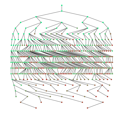
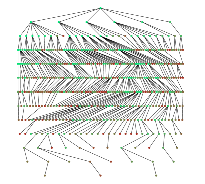
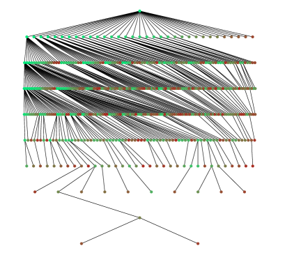
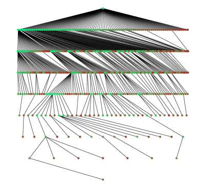
Appendix A Some pictures of sarrts

We include some pictures of sarrt for attachment random variable of the form $U^{\beta}$ for different values of $\beta$ where $U$ is uniform in $[0,1)$. We color the nodes from light (green) to dark (red) as a linear function of their labels.

Note that for small values of $\beta$, the attachment distribution concentrates more around $1$ and most of the nodes link to nodes of labels close to the bottom part of the tree. As $\beta$ becomes larger, the distribution is more concentrated near $0$. The tree has a smaller height, and the root’s degree increases.

(a) $\beta=1/2$

(b) $\beta=1$

(c) $\beta=2$

(d) $\beta=3$

Figure 1. sarrt with distribution $U^{\beta}$ and $n=500$.

Appendix B Properties of $\Lambda^{*}$ and $\Psi$

We prove some properties of Cramér’s function $\Lambda^{*}\,$ as well as the function $\Psi$ both defined in Section 3.1. See [7] for more details on Cramér’s theorem. Recall that $\Lambda^{*}$ is defined as:

$$\Lambda^{*}(z)=\sup_{\lambda\in\mathbb{R}}\big{\{}\lambda z-\Lambda(\lambda)\big{\}},\qquad\text{where}\quad\Lambda(\lambda)=\log\mathbf{E}\left\{e^{\lambda Y}\right\}.$$

Note that in our case $Y=\log X$ is a negative random variable, so $\Lambda(\lambda)<+\infty$ for $\lambda\geq 0$.

Proposition 3.

Let $Y$ be a negative random variable with $\mathbf{E}\left\{Y\right\}=-\mu\in[-\infty,0)$. Then:

1. $\Lambda^{*}\left(z\right)\in[0,+\infty]$ for all $z\in\mathbb{R}$.

2. If $\mu<+\infty$, then $-\mu\in D_{\Lambda^{*}}$ and $\Lambda^{*}(-\mu)=0$.

3. $\Lambda^{*}\left(z\right)=\sup_{\lambda\geq 0}\big{\{}\lambda z-\Lambda(\lambda)\big{\}}\quad\text{if }z\geq-\mu$.

4. If $\Lambda(\lambda)<+\infty$ for some $\lambda<0$, $\Lambda^{*}\left(z\right)=\sup_{\lambda\leq 0}\big{\{}\lambda z-\Lambda(\lambda)\big{\}}\quad\text{for }z\leq-\mu$.

5. $\Lambda^{*}$ is decreasing on $(-\infty,-\mu)$ and increasing on $(-\mu,+\infty)$.

6. $\Lambda^{*}\left(z\right)>0$ for $z>-\mu$.

7. $\Lambda^{*}$ is convex and thus continuous on the interior of $\{z:\Lambda^{*}\left(z\right)<+\infty\}$.

Proof.

1. $\Lambda^{*}\left(z\right)$ is non-negative for $z\in\mathbb{R}$:

   $$\Lambda^{*}\left(z\right)\geq 0\cdot z-\Lambda(0)=0.$$

2. By concavity of the logarithm function, we have

   (23) $$\Lambda(\lambda)=\log\mathbf{E}\left\{e^{\lambda Y}\right\}\geq\mathbf{E}\left\{\log e^{\lambda Y}\right\}=\lambda\mathbf{E}\left\{Y\right\}=-\lambda\mu,$$

   using Jensen’s inequality. As a result

   $$\Lambda^{*}\left(\mu\right)=\sup_{\lambda}\big{\{}\lambda\mu-\Lambda(\lambda)\big{\}}\leq 0.$$

   We conclude using the non-negativity of $\Lambda^{*}$.

3. If $\Lambda(\lambda)<+\infty$ for some $\lambda<0$, then $\mu<+\infty$. In fact, $\Lambda(\lambda)<+\infty$ implies

   $$\mathbf{E}\left\{Y\right\}\geq\mathbf{E}\left\{e^{-\lambda Y}\right\}/\lambda>-\infty$$

   by using the inequality $\lambda z\leq e^{\lambda z}$ for all reals $\lambda$ and $z$. It follows that if $\mu=+\infty$, $\Lambda(\lambda)=+\infty$ for all $\lambda<0$. In this case, the property trivially holds. For $\mu$ finite, $z\geq-\mu$ and $\lambda\leq 0$

   $$\lambda z-\Lambda(\lambda)\leq-\lambda\mu-\Lambda(\lambda)\leq\Lambda^{*}\left(-\mu\right)=0.$$

4. As previously shown, we have $\mu<+\infty$ in this case. For $z\leq-\mu$ and $\lambda\geq 0$,

   $$\lambda z-\Lambda(\lambda)\leq-\lambda\mu-\Lambda(\lambda)\leq\Lambda^{*}\left(-\mu\right)=0.$$

5. For $z\geq-\mu$, $\Lambda^{*}\left(z\right)=\sup_{\lambda\geq 0}\big{\{}\lambda z-\Lambda(\lambda)\big{\}}$. This implies that $\Lambda^{*}$ is increasing on $[-\mu,+\infty)$ as $z\mapsto\lambda z-\Lambda(\lambda)$ is an increasing function. Now if $\Lambda(\lambda)<+\infty$ for some $\lambda<0$, then $\Lambda^{*}\left(z\right)=\sup_{\lambda\leq 0}\big{\{}\lambda z-\Lambda(\lambda)\big{\}}$ for $z\leq-\mu$, and similarly we get $\Lambda^{*}$ decreasing on $(-\infty,-\mu)$. Otherwise if $\Lambda(\lambda)=+\infty$ for all $\lambda<0$, then $\Lambda^{*}(z)=0$ for all $z\leq-\mu$.

6. For $z>-\mu$, consider the function $f:\lambda\mapsto\lambda z-\Lambda(\lambda)$. As $Y$ is a negative random variable, this function is defined for all $\lambda\geq 0$. Moreover it is differentiable and $f^{\prime}(\lambda)=x-\mathbf{E}\left\{Ye^{\lambda Y}\right\}/\mathbf{E}\left\{e^{\lambda Y}\right\}$. Observe that $f^{\prime}(0)=z-\mu>0$. As a result $f$ is positive on a neighborhood of $0$. As a result $\Lambda^{*}\left(z\right)=\sup_{\lambda}\{f(\lambda)\}>0$ on this interval. Now as $\Lambda^{*}$ is increasing, we get the desired result.

7. For $\theta\in[0,1]$,

   $$\theta\Lambda^{*}\left(z_{1}\right)+(1-\theta)\Lambda^{*}\left(z_{2}\right) =\sup_{\lambda\in\mathbb{R}}\big{\{}\theta\lambda z_{1}-\theta\Lambda(\lambda)\big{\}}+\sup_{\lambda\in\mathbb{R}}\big{\{}(1-\theta)\lambda z_{2}-(1-\theta)\Lambda(\lambda)\big{\}}$$

   $$\geq\sup_{\lambda\in\mathbb{R}}\big{\{}\lambda(\theta z_{1}+(1-\theta)z_{2})-\Lambda(\lambda)\big{\}}$$

   $$=\Lambda^{*}\left(\theta z_{1}+(1-\theta)z_{2}\right).\qed$$

In the next proposition, another property of $\Lambda^{*}$ is introduced to prove that except in the case where $\mathcal{L}(Y)$ is a single mass, there exists $z>-\mu$ for which $\Lambda^{*}$ is finite.

Proposition 4.

Let $Y$ be a negative random variable with $\mathbf{E}\left\{Y\right\}=-\mu\in[-\infty,0)$. If $\mathcal{L}(Y)$ is not a single mass, then there exists $z>-\mu$ such that $\Lambda^{*}(z)<+\infty$. Moreover if $\Lambda(\lambda)<+\infty$ for some $\lambda<0$, then there exists also $z<-\mu$ such that $\Lambda^{*}(z)<+\infty$.

Proof.

We start by proving that $\Lambda(\lambda)/\lambda$ is a strictly increasing function for $\lambda>0$. Writing $X=e^{Y}$, we have $\log\mathbf{E}\left\{e^{\lambda Y}\right\}=\log\mathbf{E}\left\{X^{\lambda}\right\}$. Let $0<\lambda<\lambda^{\prime}$, and define $g(x)=x^{\lambda^{\prime}/\lambda}$ for $x\geq 0$. Then using Jensen’s inequality for the convex function $g$:

$$\mathbf{E}\left\{X^{\lambda}\right\}^{1/\lambda}=g\left(\mathbf{E}\left\{X^{\lambda}\right\}\right)^{1/\lambda^{\prime}}<\mathbf{E}\left\{g(X^{\lambda})\right\}^{1/\lambda^{\prime}}=\mathbf{E}\left\{X^{\lambda^{\prime}}\right\}^{1/\lambda^{\prime}}.$$

as $X$ is not constant. By taking the logarithm

$$\frac{\Lambda(\lambda)}{\lambda}<\frac{\Lambda(\lambda^{\prime})}{\lambda^{\prime}}.$$

Let $z_{1}=\Lambda(1)$. By the fact that $\Lambda(\lambda)/\lambda$ is increasing, $\lambda(z_{1}-\Lambda(\lambda)/\lambda)\leq 0$ for $\lambda\geq 1$. Thus,

$$\Lambda^{*}\left(z_{1}\right)=\sup_{\lambda\geq 0}\big{\{}\lambda(z_{1}-\Lambda(\lambda)/\lambda)\big{\}}=\sup_{0\leq\lambda\leq 1}\big{\{}\lambda z_{1}-\Lambda(\lambda)\big{\}}<+\infty.$$

Now, using equation (23), $\Lambda(0.5)/0.5\geq-\mu$. But $z_{1}=\Lambda(1)/1>\Lambda(0.5)/0.5\geq-\mu$. Finally, $z_{1}>-\mu$ and $\Lambda^{*}(z_{1})<+\infty$.

As for the case $z<-\mu$, we start by observing that $\Lambda(\lambda)/\lambda$ is a strictly decreasing function of $\lambda$ for $\lambda<0$ using the same argument as above. Then if $\Lambda(\delta)<+\infty$ for some $\delta<0$, let $z_{\delta}=\Lambda(\delta)/\delta$. We have $z_{\delta}>\Lambda(0.5\delta)/0.5\delta\geq-\mu$. Moreover, $\lambda(z_{\delta}-\Lambda(\lambda)/\lambda)\leq 0$ for $\lambda\leq\delta$. Thus,

$$\Lambda^{*}\left(z_{\delta}\right)=\sup_{\delta\leq\lambda\leq 0}\big{\{}\lambda(z_{\delta}-\Lambda(\lambda)/\lambda)\big{\}}<+\infty.\qed$$

Using these properties we prove the results needed for the function $\Psi$.

Proposition 5.

Let $Y$ be a negative random variable with $\mathbf{E}\left\{Y\right\}=-\mu\in[-\infty,0)$. Define the function $\Psi$ by $\Psi(c)=c\Lambda^{*}\left(-1/c\right)$ for $c>0$. Let $\mathcal{D}_{\Psi}=\{c>0:\Psi(c)<+\infty\}$. Then,

1. The function $\Psi$ is continuous on the interior of $\mathcal{D}_{\Psi}$. It is decreasing on $(0,1/\mu)$ and strictly increasing on $(1/\mu,+\infty)\cap\mathcal{D}_{\Psi}$.

2. The set $\{c>1/\mu:\Psi(c)>1\}$ is non-empty. Define

   $$\alpha_{\max}=\inf\left\{c>\frac{1}{\mu}:\Psi(c)>1\right\}.$$

   Then $\alpha_{\max}<+\infty$, and if $\mathcal{L}(X)$ is not a single mass, $\alpha_{\max}>1/\mu$. Moreover, for $c\in(1/\mu,\alpha_{\max})$, then $\Psi(c)<1$.

3. If $\mu<+\infty$, define

   $$\alpha_{\min}=\sup\bigg{\{}\,0\,\bigg{\}}\cup\left\{c<\frac{1}{\mu}:\Psi(c)>1\right\}.$$

   Then if $\mathcal{L}(X)$ is not a single mass, $\alpha_{\min}<1/\mu$. Moreover, for $c\in(\alpha_{\min},1/\mu)$, we have $\Psi(c)<1$.

Proof.

1. The continuity follows from the continuity of $\Lambda^{*}$. For $(1/\mu,+\infty)\cap\mathcal{D}_{\Psi}$, $\Psi$ is strictly increasing because $\Lambda^{*}$ is increasing and $\Lambda^{*}\left(z\right)>0$ for $z>-\mu$. For $(0,1/\mu)\cap\mathcal{D}_{\Psi}$, using the convexity of $\Lambda^{*}$, we have for $z<z^{\prime}\leq-\mu$ in $\mathcal{D}_{\Psi}$:

   $$\frac{\Lambda^{*}\left(z\right)}{-z}\geq\frac{\Lambda^{*}\left(z^{\prime}\right)}{-z^{\prime}}.$$

   Thus, $\Psi(-1/z)\geq\Psi(-1/z^{\prime})$ and $\Psi$ is decreasing on $(0,1/\mu)\cap\mathcal{D}_{\Psi}$.

2. Fix any $z^{\prime}\in(-\mu,0)$, then using the positivity of $\Lambda^{*}$, $\Lambda^{*}\left(z^{\prime}\right)>0$ and thus for $c\geq-1/z^{\prime}$,

   $$\Psi(c)=c\Lambda^{*}(-1/c)\geq c\Lambda^{*}(z^{\prime}).$$

   As a result, for $c$ large enough $\Psi(c)>1$. This shows that $\alpha_{\max}<+\infty$. Moreover, if $\mathcal{L}(X)$ is not a single mass, then Proposition 4 and the continuity of $\Lambda^{*}$ imply that $\Psi$ is smaller than $1$ on an interval $[1/\mu,c]$ for some $c>1/\mu$. This shows that $\alpha_{\max}>1/\mu$.

   Furthermore, taking $c<\alpha_{\max}$, by definition of $\alpha_{\max}$ and as $\Psi$ is strictly increasing on $(1/\mu,+\infty)$, $\Psi(c)<1$.

3. First, if $\Lambda(\lambda)=+\infty$ for all $\lambda<0$, then $\Lambda^{*}\left(z\right)=0$ for all $z<-\mu$. In this case, $\alpha_{\min}=0<1/\mu$ and $\Psi(c)=0<1$ for all $c\in(\alpha_{\min},1/\mu)$.

   Assume now that $\Lambda(\lambda)<+\infty$ for some $\lambda<0$. Then using Proposition 4, we have $\alpha_{\min}<1/\mu$. It remains to show that for $c\in(\alpha_{\min},1/\mu)$, $\Psi(c)<1$. Suppose for the sake of contradiction that this is not the case. Then there exists $c>\alpha_{\min}$ such that $\Psi(c)=1$. As $\Psi$ is a decreasing function in $(\alpha_{\min},1/\mu)$, this implies that there exists $z^{\prime}_{1}<z^{\prime}_{2}<1/\mu$ such that $\Lambda^{*}\left(z\right)=-z$ for all $z\in[z^{\prime}_{1},z^{\prime}_{2}]$. But for $z_{1}<z_{2}$ in $(z^{\prime}_{1},z^{\prime}_{2})$, we have

   $$\Lambda^{*}\left(\frac{z_{1}+z_{2}}{2}\right) =\sup_{\lambda\leq 0}\left\{\lambda\frac{z_{1}+z_{2}}{2}-\Lambda(\lambda)\right\}$$

   (24) $$\leq\frac{1}{2}\sup_{\lambda\leq 0}\big{\{}\lambda z_{1}-\Lambda(\lambda)\big{\}}+\frac{1}{2}\sup_{\lambda\leq 0}\big{\{}\lambda z_{2}-\Lambda(\lambda)\big{\}}$$

   $$=-\frac{z_{1}+z_{2}}{2}.$$

   So we must have equality in (iii). This means that the suprema defining $\Lambda^{*}(z_{1})$ and $\Lambda^{*}(z_{2})$ are attained at the same point. We have $\Lambda^{*}(z_{1})=\lambda z_{1}-\Lambda(\lambda)$ and $\Lambda^{*}(z_{2})=\lambda z_{2}-\Lambda(\lambda)$ for some $\lambda<0$. Observing that $\Lambda^{*}(z_{1})-\Lambda^{*}(z_{2})=\lambda(z_{1}-z_{2})$, we must have $\lambda=-1$. This implies that $\Lambda^{*}(z_{1})=-z_{1}-\Lambda(-1)=-z_{1}$. But $\Lambda(-1)=\log\mathbf{E}\left\{X^{-1}\right\}>0$. This contradicts our assumption that $\Psi(c)=1$ for some $c>\alpha_{\min}$. Note that we supposed here that for $z\in\{z_{1},z_{2}\}$ there exists some $\lambda$ such that $\Lambda^{*}\left(z\right)=\lambda z-\Lambda(\lambda)$. In the next paragraph, we show that we can suppose this is the case.

   Fix some $z\in[z_{1},z_{2}]$. We want to show that there exists a $\lambda\leq 0$ such that $\Lambda^{*}\left(z\right)=\lambda z-\Lambda(\lambda)$. Consider $\mathcal{D}_{\Lambda}=\{\lambda\in\mathbb{R}:\Lambda(\lambda)<+\infty\}$ and let $a=\inf\mathcal{D}_{\Lambda}$. Suppose first $a>-\infty$, and consider the limit $\ell=\lim_{\lambda\downarrow a}\Lambda(\lambda)$. This limit exists because $\Lambda$ is a decreasing function of $\lambda$. If $\ell<+\infty$, then by extending $\Lambda$ by continuity, $\Lambda^{*}\left(z\right)=\sup_{a\leq\lambda\leq 0}\{\lambda z-\Lambda(\lambda)\}$ so we can assume that the supremum is attained. If $\ell=+\infty$, then there exists $a_{1}$ such that $\Lambda(\lambda)\geq az$ for $\lambda<a_{1}$. Thus, we have $\Lambda^{*}\left(z\right)=\sup_{a_{1}\leq\lambda\leq 0}\{\lambda z-\Lambda(\lambda)\}$, and the supremum is also attained in this case. Now suppose that $a=-\infty$ and define similarly $\ell=\lim_{\lambda\to-\infty}\Lambda(\lambda)$. If $\ell<+\infty$, then $\Lambda^{*}(z)=+\infty$ which is a contradiction. The last case is $\ell=+\infty$. As $\Lambda$ is a convex function, the function $\varphi:\lambda\mapsto\lambda z-\Lambda(\lambda)$ is a concave function so it is monotone for $\lambda\leq\lambda_{0}$ small enough. If it is increasing, then $\Lambda^{*}\left(z\right)=\sup_{\lambda_{0}\leq\lambda\leq 0}\{\lambda z-\Lambda(\lambda)\}$ and we are done. If $\varphi$ is decreasing for $\lambda\leq\lambda_{0}$, then we can suppose $\Lambda^{*}\left(z\right)=\lim_{\lambda\to-\infty}\lambda z-\Lambda(\lambda)$ and by assumption $\Lambda^{*}\left(z\right)=-z$. But then for $z^{\prime}_{1}<z$, we have $\Lambda^{*}(z^{\prime}_{1})\leq\lim_{\lambda\to-\infty}\lambda(z^{\prime}_{1}-z)+\lambda z-\Lambda(\lambda)=+\infty$, which contradicts the fact that $\Lambda(z^{\prime}_{1})=-z^{\prime}_{1}$.

∎

References

- Andersen [1953] E. Andersen. On the fluctuations of sums of random variables. Mathematica Scandinavica, 1:263–285, 1953.
- Arya et al. [1999] S. Arya, M. Golin, and K. Mehlhorn. On the expected depth of random circuits. Combinatorics, Probability and Computing, 8:209–228, 1999.
- Barabasi and Albert [1999] A. Barabasi and R. Albert. Emergence of scaling in random networks. Science, 286:509–512, 1999.
- Chernoff [1952] H. Chernoff. A measure of asymptotic efficiency for tests of a hypothesis based on the sum of observations. The Annals of Mathematical Statistics, 23:493–507, 1952.
- Chung and Erdős [1952] K. Chung and P. Erdős. On the application of the Borel-Cantelli lemma. Transactions of the American Mathematical Society, pages 179–186, 1952.
- Cramér [1938] H. Cramér. Sur un nouveau théorème-limite de la théorie des probabilités. Actualités Scientifiques et Industrielles, 736:5–23, 1938.
- Dembo and Zeitouni [1998] A. Dembo and O. Zeitouni. Large Deviations Techniques and Applications. Springer Verlag, 1998.
- Devroye [1986] L. Devroye. A note on the height of binary search trees. Journal of the ACM, 33(3):489–498, 1986.
- Devroye [1987] L. Devroye. Branching processes in the analysis of the heights of trees. Acta Informatica, 24(3):277–298, 1987.
- Devroye and Janson [2011] L. Devroye and S. Janson. Long and short paths in uniform random recursive dags. Arkiv för Matematik, 49:61–77, 2011. URL http://arxiv.org/abs/0906.0152v1.
- Devroye and Lu [1995] L. Devroye and J. Lu. The strong convergence of maximal degrees in uniform random recursive trees and dags. Random Structures and Algorithms, 7(1):1–14, 1995.
- Devroye and Reed [1995] L. Devroye and B. Reed. On the variance of the height of random binary search trees. SIAM Journal on Computing, 24:1157–1162, 1995.
- Dobrow [1996] R. Dobrow. On the distribution of distances in recursive trees. Journal of Applied Probability, 33(3):749–757, 1996.
- Dobrow and Fill [1999] R. Dobrow and J. Fill. Total path length for random recursive trees. Combinatorics, Probability and Computing, 8(04):317–333, 1999.
- Drmota [2009] M. Drmota. Random trees: an interplay between combinatorics and probability. Springer, 2009.
- D’Souza et al. [2007] R. M. D’Souza, P. L. Krapivsky, and C. Moore. The power of choice of choice in growing trees. The European Physical Journal B - Condensed Matter and Complex Systems, 59(4):535–543, 2007.
- Dwass [1969] M. Dwass. The total progeny in a branching process and a related random walk. Journal of Applied Probability, 6(3):682–686, 1969.
- Gastwirth [1977] J. L. Gastwirth. A probability model of a pyramid scheme. The American Statistician, 31(2):79–82, 1977.
- Hoeffding [1963] W. Hoeffding. Probability inequalities for sums of bounded random variables. Journal of the American Statistical Association, 58:13–30, 1963.
- Mahmoud [1992] H. Mahmoud. Distances in random plane-oriented recursive trees. Journal of Computational and Applied Mathematics, 41(1-2):237–245, 1992.
- Mahmoud [2010] H. Mahmoud. The power of choice in the construction of recursive trees. Methodology and Computing in Applied Probability, 12:763–773, 2010.
- Meir and Moon [1978] A. Meir and J. Moon. On the altitude of nodes in random trees. Canadian Journal of Mathematics, 30:997–1015, 1978.
- Moon [1974] J. Moon. The distance between nodes in recursive trees. London Mathematical Society Lecture Notes, 13:125–132, 1974.
- Na and Rapoport [1970] H. Na and A. Rapoport. Distribution of nodes of a tree by degree. Mathematical Biosciences, 6:313–329, 1970.
- Neininger [2002] R. Neininger. The Wiener index of random trees. Combinatorics, Probability and Computing, 11(06):587–597, 2002.
- Pittel [1994] B. Pittel. Note on the heights of random recursive trees and random m-ary search trees. Random Structures and Algorithms, 5:337–348, 1994.
- Ross [1996] S. Ross. Stochastic processes. Wiley New York, 1996.
- Smythe and Mahmoud [1995] R. Smythe and H. Mahmoud. A survey of recursive trees. Theory of Probability and Mathematical Statistics, 51:1–27, 1995.
- Su et al. [2006] C. Su, Q. Feng, and Z. Hu. Uniform recursive trees: Branching structure and simple random downward walk. Journal of Mathematical Analysis and Applications, 315(1):225–243, 2006.
- Szymański [1987] J. Szymański. On a nonuniform random recursive tree. In Random Graphs’ 85: Based on Lectures Presented at the 2nd International Seminar on Random Graphs and Probabilistic Methods in Combinatorics, volume 33, pages 297–306. North-Holland, 1987.
- Szymański [1990] J. Szymański. On the maximum degree and the height of a random recursive tree. In M. Karoński, J.Jaworski, and A.Ruciński, editors, Random Graphs ’87, pages 313–324. Wiley, 1990.
- Tsukiji and Xhafa [1996] T. Tsukiji and F. Xhafa. On the depth of randomly generated circuits. In Proceedings of Fourth European Symposium on Algorithms, pages 208–220, 1996.