On the description of two-particle transfer in superfluid systems

Abstract

Exact results of pair transfer probabilities for the Richardson model with equidistant or random level spacing are presented. The results are then compared either to particle-particle random phase approximation (ppRPA) in the normal phase or quasi-particle random phase approximation (QRPA) in the superfluid phase. We show that both ppRPA and QRPA are globally well reproducing the exact case although some differences are seen in the superfluid case. In particular the QRPA overestimates the pair transfer probabilities to excited states in the vicinity of the normal-superfluid phase transition, which might explain the difficult in detecting collective pairing phenomena as for example the Giant Pairing Vibration. The shortcoming of QRPA can be traced back to the breaking of particle number that is used to incorporate pairing. A method, based on direct diagonalization of the Hamiltonian in the space of two quasi-particle projected onto good particle number is shown to improve the description of pair transfer probabilities in superfluid systems.

I Introduction

The importance of pairing correlations in nuclear systems has been established in several aspects, binding energies of nuclei, odd-even effects, superfluid phenomena and pair transfer mechanisms, to mention just a few. However, despite the fact that pairing is anticipated to play a significant role in the pair transfer process, the existence of collective effects, like Giant Pair Vibration (GPV) Bro73 ; Oer01 ; Pot09 ; Kha04 ; Kha09 ; Ave08 leading to an increase in the pair transfer from a superfluid nuclei still challenges the experimental nuclear physics Mou11 . On the theoretical side, mean-field methods based on Hartree-Fock-Bogolyubov (HFB) sometimes augmented by Quasi-particle Random Phase Approximation (QRPA) have been used to predict pair transfer probabilities either from ground state to ground state or from ground state to excited states Dob96 ; Shi11 ; Pot11 ; Pll11 ; Gra12 . A common conclusion of most of these studies is the sensitivity of one- or two-nucleon transfer process to the internal topology of pairing in nuclei. In the present work, exact results of pair transfer probability are obtained for the Richardson model Ric64 consisting in set of single-particle levels interacting through a pure pairing interaction. This model can be seen as the valence space of the last occupied level in nuclei where nucleons can be either added (pick-up reactions) or removed (stripping reactions). The possibility to perform exact calculations open new perspectives to understand the pair transfer process and provides a benchmark for approximate treatments. In the following, we first discuss the pair transfer mechanism from a general point of view and estimate pair transfer probabilities in the pairing model.

We are interested here in a process where two particles are either added or removed in a system that is initially in its ground state formed of N particles. In the following, we denote by $|\nu,A\rangle$ respectively the eigenstates of the systems with $A$ particles associated to the set of energies $E^{A}_{\nu}$ and, by convention, $\nu=0$ is taken for ground state. During its evolution, the system wave-function can be decomposed as Rip69

$$|\Psi(t)\rangle = e^{-itE^{N}_{0}/\hbar}\left\{\sum_{\nu}c^{N}_{\nu}e^{-it(E^{N}_{\nu}-E^{N}_{0})/\hbar}|\nu,N\rangle\right.$$

$$\phantom{e^{-itE^{N}_{0}}}+\sum_{\nu}c^{N-2}_{\nu}e^{-it(E^{N-2}_{\nu}-E^{N}_{0})/\hbar}|\nu,N-2\rangle$$

$$\phantom{e^{-itE^{N}_{0}}}+\left.\sum_{\nu}c^{N+2}_{\nu}e^{-it(E^{N+2}_{\nu}-E^{N}_{0})/\hbar}|\nu,N+2\rangle\right\}$$

where the first line describes the possibility that the system remains in its ground state or in one of its excited states without changing its particle number. Second (resp. third) line contains the information on the removal and/or addition process. The explicit form of the coefficients $c^{A}_{\nu}$ depends on the physical process under interest, like the stripping or pick-up reactions in nuclear physics. On the theoretical side, information of these processes can be obtained by studying the small amplitude response of the system to an external field $\hat{T}$ that changes the particle number by two units. Then, information on the transfer reduces to the knowledge of the response function, given by:

$$S(E) = \sum_{\nu}|\langle N+2,\nu|\hat{T}|N,0\rangle|^{2}\delta\left(E-\Delta E^{N+2}_{\nu}\right)$$

$$+ \sum_{\nu}|\langle N-2,\nu|\hat{T}|N,0\rangle|^{2}\delta\left(E-\Delta E^{N-2}_{\nu}\right)$$

$$\equiv S^{\rm Add}(E)+S^{\rm Rem}(E)$$

where $\Delta E^{N\pm 2}_{\nu}=E^{N\pm 2}_{\nu}-E^{N}_{0}$. In the following, $S^{\rm Add}(E)$ (resp. $S^{\rm Rem}(E)$) will be referred to addition (removal) strength function. A common choice of $\hat{T}$ Ave08 to excite pairing modes is

$$\hat{T} = \sum_{i}(T_{i\bar{i}}a^{\dagger}_{i}a^{\dagger}_{\bar{i}}+T^{*}_{i\bar{i}}a_{\bar{i}}a_{i})$$ (2)

where $a^{\dagger}_{i}a^{\dagger}_{\bar{i}}$ corresponds to creation operators of a pair of time-reversed single-particle states. In the present article, we are interested in a physical process where two-particles are either added or removed. In that case, it is more suited to consider directly the non-Hermitian addition (resp. removal) transition operator, denoted by $\hat{T}^{\rm Add}$ (resp. $\hat{T}^{\rm Rem}$) defined through

$$\hat{T}^{\rm Add} = \sum_{i}T_{i\bar{i}}a^{\dagger}_{i}a^{\dagger}_{\bar{i}},~{}~{}~{}\hat{T}^{\rm Rem}=\sum_{i}T^{*}_{i\bar{i}}a_{\bar{i}}a_{i}$$ (3)

respectively associated to $S^{\rm Add}(E)$ and $S^{\rm Rem}(E)$. From the expression of the strength, we see that the understanding of the two-particle transfer passes through a good knowledge of the spectroscopy of initial and final states as well as of the capacity to provide the addition or removal probabilities defined here as:

$$P^{\rm Add}_{\nu} = |\langle N+2,\nu|\hat{T}|N,0\rangle|^{2},$$ (4)

$$P^{\rm Rem}_{\nu} = |\langle N-2,\nu|\hat{T}|N,0\rangle|^{2}.$$ (5)

If the many-body problem can be solved exactly, such quantities as well as the exact eigenvalues of the Hamiltonian can be used to have a precise estimate of the strength function (I). In most realistic situations, such treatment is impossible and educated guess should be used. In the present work, we are interested in an initial system where pairing correlation plays a role. This case has been first considered in refs. Bes66 ; Bro68 ; Bro73 leading to the concept of pairing vibration, i.e. a coherent excitation of pairs of particles that is expected to show up in the enhancement of pair transfer probabilities. The standard way to incorporate pairing correlation is to use the BCS or HFB approach as a starting point Rin80 ; Bla86 . This technique is indeed standardly used in nuclear physics either to estimate the transfer from ground state to ground state Mat10 ; Shi11 ; Gra12 or from ground state to excited states. In the latter case, the response is obtained using QRPA Kha04 ; Kha09 ; Pll11 or its time-dependent version Ave08 . For a comprehensive introduction, please refer to Bri05 .

With the increase of computational powers, it is possible nowadays to study exactly pair transfer in schematic model that approaches realistic situations and to quantify the predictive power of mean-field based approaches. In the present work, we first present exact results of pair transfer probabilities for the Richardson model with equidistant or random level spacing. The exact results are then used to benchmark standard approaches, namely ppRPA and QRPA.

II Exact description in the Richardson model

A system of $\Omega$ doubly-degenerated single-particle levels interacting via a pairing force with parameter $G$ is considered. The Hamiltonian is given by Ric64

$$H=\sum_{i=1}^{\Omega}\epsilon_{i}\hat{N}_{i}-G\sum_{i,j=1}^{\Omega}\hat{P}_{i}^{\dagger}\hat{P}_{j}~{},$$ (6)

where the particle-number operator $\hat{N}_{i}$ and pair creation/annihilation operators $\hat{P}_{i}^{\dagger}$, $\hat{P}_{i}$ are given by

$$\hat{N}_{i}=a_{i}^{\dagger}a_{i}+a_{\bar{i}}^{\dagger}a_{\bar{i}}~{},\hskip 14.22636pt\hat{P}_{i}^{\dagger}=a_{i}^{\dagger}a_{\bar{i}}^{\dagger}~{},~{}~{}~{}~{}\hat{P}_{i}=(\hat{P}_{i}^{\dagger})^{\dagger}~{}.$$ (7)

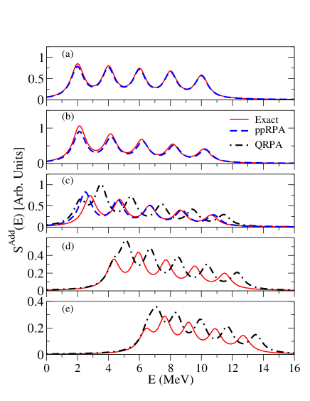
Figure 1: (color online) Addition strength function as a function of the excitation energy $E$ for different pairing strength G obtained using exact eigenvalues and eigenstates in Eq. (I) (red solid line) for a system of $N=8$ particles to $N=10$ in the case of $\Omega=10$ equally spaced levels. From top to bottom: (a) $G/\Delta\varepsilon=0.1$ , (b) $0.3$, (c) $0.5$, (d) $0.7$ and (e) $0.9$ are shown. The results of the ppRPA (blue dashed line) and QRPA (black dot-dashed line) are also presented. Note that in panel (c), the result of ppRPA obtained at the collapse point $G=0.48\Delta\varepsilon$ is also reported. The QRPA are shown only above the BCS threshold $G=0.33\Delta\varepsilon$.

For not too large model space $\Omega$, exact solutions can be obtained using standard diagonalization techniques in subspace of given seniority Zel03 . As a test case here, a system of $N=8$ particles with $\Omega=10$ doubly degenerated levels is considered here. Assuming a simple transition operator (2) with $T_{i\bar{i}}=1$ for all pairs, illustrations of addition strength function obtained for the Richardson model are shown in Fig. 1, in full (red) line, for equidistant level spacing, i.e. $\epsilon_{i}=i\Delta\varepsilon$ ($i=1$, $\Omega$), for different values of the pairing interaction and $\Delta\varepsilon=1$ MeV. In the following the excitation energies will be calculated with respect to the ground state of the system with $N=10$ particles consistently in all the theories. The presented result is exact in the sense that the exact eigenvalues and eigenstates of the system with $N=8$ and $N=10$ have been used to compute Eq. (I). Note that in the present work, we are mainly interested in the transition from ground state to excited states of the $N+2$ nucleus and the contribution of the ground state to ground state transfer has been omitted in the figure. Moreover, in order to make simpler the comparison between different results, we have folded the discrete spectra with a Lorentzian function with a width of 1 MeV. For completeness, we also show in Fig. 2 similar results obtained with randomly spaced system whose single-particle energy are $0.551$, $2.176$, $4.033$, $5.142$, $6.444$, $7.029$, $7.827$, $8.343$, $9.226$ and $9.571$ in MeV units. This situation could be considered closer to realistic cases.

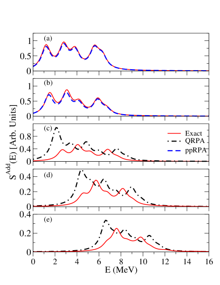
Figure 2: (color online) Same as figure 1 obtained for randomly spaced single-particle energies. See the text for more details. The QRPA are shown only above the BCS threshold $G=0.44$ MeV.

In the exact calculations, we observe a shift of the excitation spectrum toward higher energies as the pairing strength $G$ increases while the pair transfer probabilities of the excited states get smaller. On the contrary, as it will be shown below, the pair transfer probability from ground state to ground state increases as $G$ increases.

III ppRPA vs QRPA approaches to pair transfer

As already mentioned, in most cases, exact evaluation of the pair transfer probabilities cannot be performed and approximations for the many-body states are necessary. The most common strategy used in nuclear physics is to first apply the HFB or BCS theory and minimize the energy in the Hilbert space of quasi-particle vacuum imposing a mean particle number equal to $N$. This leads to an approximation for $|0,N\rangle$. Using standard notations, the quasi-particle vacuum is given by

$$|0,N\rangle\simeq|0,{\rm QP}\rangle=\prod_{i}\left[\alpha_{i}^{\dagger}\alpha_{\bar{i}}^{\dagger}\right]|-\rangle$$ (8)

where $|-\rangle$ is the quasi-particle vacuum and $\alpha_{i}$ is the quasi-particle annihilation operator defined through the simple Bogolyubov transformation:

$$\alpha_{i} = U_{i}a_{i}-V_{i}a^{\dagger}_{\bar{i}}$$ (9)

$$\alpha_{\bar{i}} = U_{i}a_{\bar{i}}+V_{i}a^{\dagger}_{i}.$$ (10)

In the HFB approach, the above transformation automatically implies that the single-particle basis identifies with the canonical basis.

In the present model, the Hamiltonian (6) is already written in the canonical basis for the HFB theory. This theory is particularly suitable to provide estimates for ground state (GS) to GS transfer probabilities Shi11 ; Gra12 . Since we want to compare with exact results, at the BCS/HFB and QRPA level the contribution to the particle-hole channel of the pairing interaction is taken into account. The result of the HFB theory for this probability is shown in figure 3 and compared to the exact solution. Note that below the pairing threshold (denoted by $G_{\rm cr}$ and equal to 0.33 MeV and 0.44 MeV for the $8$ particles system in the equally spaced and random spaced case, respectively), the HFB reduces to HF and probability is $1$. As illustrated in this figure, while the HF theory (not shown) would have failed to reproduce the exact probabilities, the HFB framework gives estimations that are already rather close to the exact ones in the superfluid regime.

Due to the absence of residual coupling between quasi-particle excitations, it is known that HFB alone cannot properly describe excited states. Then, linear response theory including possible particle-particle (pp), hole-hole (hh), or particle-hole (ph) excitations is applied to describe excited states, and then transfer probabilities, within the QRPA approach. In QRPA, the excited states, denoted by $|\nu\rangle$, are obtained by considering coherent superposition of 2 quasi-particle (2QP) excitations. This leads to

$$|\nu\rangle = Q_{\nu}^{\dagger}|0\rangle,$$ (11)

where $Q_{\nu}^{\dagger}$ are QRPA phonons written as

$$Q_{\nu}^{\dagger}=\sum_{i}(X_{j}^{\nu}\alpha^{\dagger}_{i}\alpha^{\dagger}_{\bar{i}}-Y_{j}^{\nu}\alpha_{\bar{i}}\alpha_{i}),\hskip 14.22636ptQ_{\nu}=(Q_{\nu}^{\dagger})^{\dagger},$$ (12)

while $|0\rangle$ is the phonon vacuum, defined through the conditions $Q_{\nu}|0\rangle=0$. In practice, the components $X^{\nu}$ and $Y^{\nu}$ as well as the energies of the excited states $\omega_{\nu}$ are deduced by solving the QRPA eigenvalue problem Row10 . Since these techniques are rather standard Rin80 , we only recall here the expressions of the pair transfer probability.

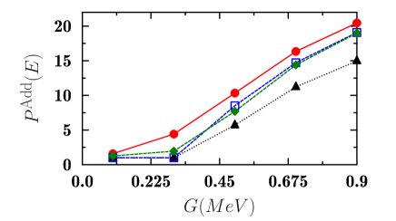
Figure 3: (color online) Illustration of the application of mean-field theory to provide estimate of ground state to ground state addition pair probability. The exact result (red circles), BCS (black triangles) and BCS projected on good particle number (blue open squares) are shown here for the equidistant single-particle level case. The result of the P-QTDA^(GS) is also presented with green filled diamond.

In QRPA, the addition transition probability is given by

$$P^{\rm Add}_{\nu}=|\langle 0|\hat{T}^{\rm Add}|\nu\rangle|^{2}=|\sum_{i}(V^{2}_{i}X_{i}^{(\nu)}-U^{2}_{i}Y_{i}^{(\nu)})|^{2}.$$ (13)

It is well known that, the first solution of the QRPA equations corresponds to the spurious mode, which is then not considered in the evaluation of the strength function.

In the weak coupling limit, below a certain threshold value of $G$ denoted by $G_{\rm cr}$, the minimization of the energy in HFB identifies to the Hartree-Fock approach with no pairing. Then the mean-field vacuum is a pure Slater determinant where the lowest hole states are occupied. In this case, labeling by $h$ the hole state ($V_{h}$ = 1, $U_{h}=0$) and $p$ ($V_{p}=1$, $U_{p}=1$) the particle states associated to this vacuum, the excited states are described by using the particle-particle RPA (ppRPA) where the phonon creation operators (12) can be written as

$$Q_{\nu}^{\dagger} = \sum_{p}X_{p}^{\nu}a^{\dagger}_{p}a^{\dagger}_{\bar{p}}+\sum_{h}Y_{h}^{\nu}a^{\dagger}_{h}a^{\dagger}_{\bar{h}},$$ (14)

while the addition probability simply writes:

$$P^{\rm Add}_{\nu} = |\sum_{p}X_{p}^{\nu}-\sum_{h}Y_{h}^{\nu}|^{2}.$$ (15)

Note that in the ppRPA case, contrary to the QRPA, the $U(1)$ symmetry associated to particle number conservation is not broken. Explicit forms of the ppRPA and QRPA equations for the model considered here can be found in Refs. Gam06 ; Dan06 ; Dan07

In Figs 1 and 2, the ppRPA (dashed line) and QRPA (dot-dashed line) are compared to the exact results. Above a given threshold $G_{cr}^{RPA}$, ppRPA collapses and leads to imaginary energies making not possible a direct comparison with the exact and QRPA results. However, in Fig. 1 we show in the panel (c) corresponding to a pairing strength $G=0.5MeV$ the ppRPA results obtained at the collapse point, i.e. $G_{cr}^{RPA}=0.48$, in order to show that its description is still reasonable even in the superfluid phase.

From these comparisons, the following conclusions can be drawn: (i) The ppRPA does reproduce perfectly the exact results (energies and probabilities) in the normal phase. (ii) The QRPA provides a global reproduction of the pair transfer probabilities in the superfluid phase. In particular, the threshold in energy that is directly related to pairing correlation is properly accounted for. It is worth to mention, that such a threshold can only be described in a mean-field theory by breaking particle number symmetry. Finally, it is also clearly seen that some differences exist between the exact and QRPA. in general QRPA leads to peaks in the strength that are at slightly higher energies compared to the exact solution while probabilities are slightly overestimated. These differences are even stronger in the random space case and can stem from different origins. First, while part of the four quasi-particles (4QP) are accounted for in the QRPA ground state correlations, the complete inclusion of 4QP excitations is known to modify excited state energy spectrum Rin80 ; Lac12 . Second, a systematic error exists due to the breaking of particle number. Panel (c) of Fig. 1 illustrated that when ppRPA is applicable in the superfluid phase $G\leq 0.48$ MeV, it gives a better agreement with the exact result compared to QRPA. Since ppRPA is a particle number conserving theory, this is a first indication that the breaking of $U(1)$ symmetry might pollute the QRPA predictions.

III.1 Role of particle number in the estimation of pair transfer probabilities

At this stage, it is most likely to conjecture that the failure of QRPA to reproduce two-particle transfer processes stems from the mixing of systems with different particle numbers. The QRPA approach implicitly assumes that the states $|\nu\rangle$ are relatively good approximations for the eigenstates of systems with $N+2$ (or $N-2$) particles. As an illustration of the correctness of this assumption, the mean number of particles $N_{\nu}=\langle\nu|\hat{N}|\nu\rangle$ is displayed in the bottom panel of Fig. 4 as a function of the excitation energy $\omega_{\nu}$ . $N_{\nu}$ has been estimated using the quasi-boson approximation leading to:

$$N_{\nu}=\sum_{i}2(U_{i}^{2}-V_{i}^{2})(X_{i}^{\nu 2}+Y_{i}^{\nu 2})+\langle\hat{N}\rangle,$$ (16)

where $\langle\hat{N}\rangle$ is the number of particle in the QP vacuum.

In the same figure, the mean-particle number of the two quasi-particle (2QP) excited states $|k\rangle$ as a function of $(\epsilon_{k}-\lambda)$ is also shown, where $\lambda$ is the Fermi energy. The 2QP states are defined through:

$$|k\rangle = \alpha^{\dagger}_{k}\alpha^{\dagger}_{\bar{k}}|0,QP\rangle,$$ (17)

where the ground state has $N$ particles in average. The mean particle number in $|k\rangle$ is given by:

$$N_{k}=\langle k|\hat{N}|k\rangle = \langle\hat{N}\rangle+2U^{2}_{k}-2V^{2}_{k}.$$ (18)

This expression as well as the illustration in Figure 4 clearly shows that the 2QP states will be close to a state with $N+2$ (resp. $N-2$) particles only if $U_{k}\rightarrow 1$, i.e. well above the Fermi energy $\lambda$ (resp. $U_{k}\rightarrow 0$, i.e. well below the Fermi energy), but will be a bad approximation if the 2QP state involves single-particle state in the vicinity of $\lambda$. Consequently, QRPA states will also suffer from the same problems if the state is constructed from 2QP states that are close to the Fermi energy. While the QRPA results are in a reasonable agreement with the exact case, the effect of particle number conservation on the pair transfer is largely uncontrolled within QRPA. This is anticipated to be especially crucial in exotic nuclei as the level spacing is reduced closed to the drip line.

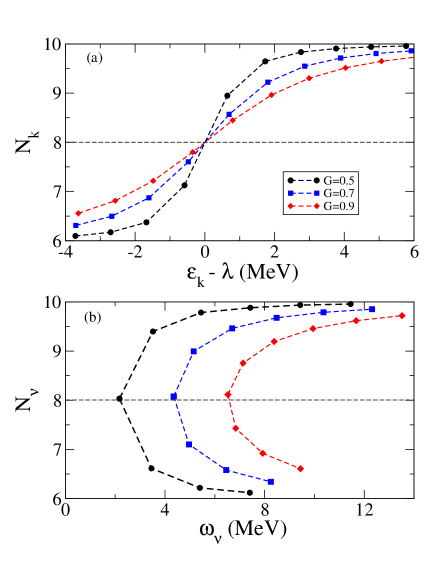
Figure 4: (color online) Bottom: mean number of particles $N_{\nu}$ of the QRPA states as a function of their excitation energy $\hbar\omega_{\nu}$. Top: mean number of particles $N_{k}$ of $2$QP states as a function of $(\epsilon_{k}-\lambda)$, where $\lambda$ is the Fermi energy.

IV Improved treatment of pair transfer in superfluid systems

The effect of particle number conservation on pair transfer from ground state to ground state has been already studied in Ref. Gra12 . It has been empirically found that the breaking of $U(1)$ symmetry has a rather small impact on the estimated probabilities. As a further illustration, we show in Figure 3 estimations of transfer probabilities with equation (4) using the ground state quasi-particle vacua projected either on $N$ or on $N+2$ particle numbers (see Ref. Gra12 for technical details). As seen in Fig. 3, the BCS approach reduces to HF below the threshold and is not able to reproduce the transfer probability at low G. The projection after variation (open square) obviously does not cure this problem but considerably improves the probability above the threshold especially in the strong coupling regime. Note that As a conclusion, the HFB and/or BCS approach augmented by an a posteriori projection is already very good to describe GS to GS transition in the superfluid regime. Therefore, in the following we will concentrate the discussion on excited state where it is necessary to go beyond HFB.

From previous discussion, we are facing the following dilemma: to describe the physics of pairing and in particular the gap in energy between the ground state and the first excited state in a superfluid system, it is necessary to break the $U(1)$ symmetry. On the other hand, this symmetry breaking seems to be at the origin of some discrepancies between QRPA and exact pair transfer probabilities.

The most direct extension of the projection technique to estimate transition from ground state to ground state would be to directly estimate the transition from the BCS/HFB ground state projected onto $N$ particle to the QRPA eigenstates projected onto $N+2$ particles. This has however two disadvantages (i) in practice we found that the pair transfer probabilities that are much smaller than the exact ones (ii) QRPA states are not anymore orthogonal after projection leading to some difficulties to interpret the probabilities themselves.

Alternatively, one can try to develop a RPA like approach directly in the space of projected 2QP states. Following the Tamm-Dancoff approximation spirit, a set of states $|\Phi_{k}\rangle$ defined through:

$$|\Phi_{k}\rangle = \hat{P}_{N+2}\alpha^{\dagger}_{k}\alpha^{\dagger}_{\bar{k}}|0,QP\rangle.$$ (19)

are introduced, where $\hat{P}_{N+2}$ is the projector on $N+2$ particles Bla86 . Then, excited states of the system with $N+2$ particles decompose as

$$|\nu,N+2\rangle=\sum_{k}X^{\nu}_{k}|\Phi_{k}\rangle.$$ (20)

This strategy has been analyzed in Ref. Kyo90 as well as its RPA generalization following Refs. Sch89 (see also Rad05 ).

A proper description would require a full Projected QRPA calculation whose practical implementation would be rather cumbersome, especially in realistic calculations. A simpler approach is to introduce what could be considered as a projected version of a two quasiparticle Tamm-Dancoff approximation. Again, it should be mentioned that contrary to standard TDA, states $|\Phi_{k}\rangle$ are neither normalized nor orthogonal with each others. Therefore, a special attention has to be paid when formulating the approach. In practice, this implies to diagonalize the overlap matrix $O_{kl}=\langle\Phi_{k}|\Phi_{l}\rangle$ prior to write the TDA eigenvalue problem. A practical method, has been proposed in ref. Kyo90 to obtain the TDA equation in the projected space. Following Kyo90 , the excited states are written in terms of new states

$$|\nu,N+2\rangle=\sum_{k}X^{\nu}_{k}|(\Phi_{k})\rangle.$$ (21)

States $|(\Phi_{k})\rangle$ are defined though:

$$|(\Phi_{k})\rangle = |\Phi_{k}\rangle-\langle 0_{\rm N+2}|\Phi_{k}\rangle,$$ (22)

where $|0_{\rm N+2}\rangle$ correspond here to the approximated ground state with $N+2$ particles. While in the original article, this ground state was anticipated to be obtained with a Variation After Projection (VAP) procedure, below it is simply taken as $|0_{\rm N+2}\rangle\simeq\hat{P}_{N+2}|0,{\rm QP}\rangle$. Then the TDA eigen-equation is solved in the space of $|(\Phi_{k})\rangle$ states. In the following, this approach is referred to Projected two Quasi-Particle TDA (P-QTDA).

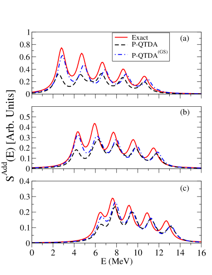
Figure 5: (color online) (color online) Same as figure 1 for (a) $G=0.5$ MeV, (b) $G=0.7$ MeV and (c) $G=0.9$ MeV. The exact result (red solid line) is compared to the P-QTDA (black dashed line) and P-QTDA^(GS) (blue dot-dashed line).

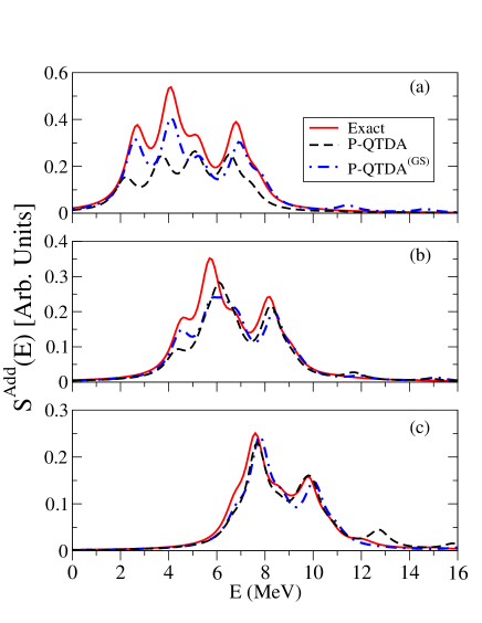
Figure 6: (color online) Same as figure 5 for the case of random level spacing.

Consistently with the present approach, addition pair transfer probabilities are computed using the expectation value of the transition operator between the quasi-particle vacuum projected on particle $N$ and the excited states (21):

$$P^{\rm Add}=\left|\sum_{\nu}X^{\nu}_{k}\langle 0,{\rm QP}|\hat{P}_{N}\hat{T}\hat{P}_{N+2}|(\Phi_{k})\rangle\right|^{2}.$$ (23)

The projection onto different particle numbers in the expression does not induce extra difficulty using the fact that

$$\langle 0,{\rm QP}|\hat{P}_{N}\hat{T}\hat{P}_{N+2}|\Phi_{k}\rangle = \langle 0,{\rm QP}|\hat{T}\hat{P}_{N+2}|\Phi_{k}\rangle$$

$$= \langle 0,{\rm QP}|\hat{P}_{N}\hat{T}|\Phi_{k}\rangle.$$

Therefore expectation values entering in expression (23) can be performed using standard projections techniques. In practice, the projection on particle number is made by discretizing the gauge angle integration using the Fomenko approach with 199 points Fom70 ; Ben09 . Useful expression to express the overlaps as well as the Hamiltonian expectation value in a projected basis can be found in the appendix of Ref. Lac12 .

Illustration of the method proposed in ref. Kyo90 applied to pair transfer are shown in Fig. 5 and Fig. 6 respectively for the equidistant and random single-particle level spacing. These figures clearly demonstrate that the projected TDA approach provides a much better description of the energy peak positions of the excited states in the system with $N+2$ particles. However, probabilities of transfer are underestimated especially as $G$ decreases.

Further improvements can a priori be made by including more correlations in the ground state $|0_{\rm N+2}\rangle$. Here, we simply used a Projection After Variation (PAV) approach to approximate this state. A better treatment would be to perform a VAP as originally proposed in ref. Kyo90 . Further correlations, like correlations induced by the coupling to 4QP states might be included using Projected QRPA instead of Projected TDA approach. The Projected QRPA approach has also been formulated previously (section III-B of Ref. Kyo90 ). In that case, not only the projected 2QP states but also the projected 4QP states should be explicitly introduced.

The use of VAP and/or the introduction of 4QP, although possible in the present model San08 ; Hup11 ; Lac12 , will considerably increase the complexity of the approach in realistic situations (see for instance Rod07 ; Rod10 ; Hup12 for the VAP). Below, we propose a simpler method inspired from P-QTDA and able to grasp part of the ground state correlations without increasing the numerical complexity.

Contrary to standard linear response theory based on HF (resp. HFB), the ground state projected onto good particle number is not orthogonal to the particle-hole (resp. 2QP) excited states. Similarly, the projected 2QP states are themselves not orthogonal to the projected 4QP or higher order excitations. At first glance, this might be seen as a disadvantage compared to RPA or QRPA since additional orthonormalization is required. On the contrary, one might take advantage of the presence of higher order components to improve the description of the GS itself.

The aim of the P-QTDA approach was to describe excitations with respect to the projected ground state. Then, the latter state has been naturally removed before solving the eigenvalues equation (Eq. (22)). Let us assume that we restart from expression (20) where the projected mean-field is also included in the sum ( with the convention that $|\Phi_{0}\rangle=\hat{P}_{N+2}|0,QP\rangle$). Then, coefficients $X^{\nu}_{k}$ can be obtained by diagonalizing the hamiltonian in the $\{\Phi_{k}\}$ (with proper treatment of the non-orthonormality of the states). This direct approach, called below P-QTDA^(GS), not only provides a way to get excited states but might also improve the description of the ground state itself. This is indeed what we observed empirically. For instance, for $G=0.5$ MeV and equidistant level spacing, the new ground state has an energy $300$ keV lower than the energy of the original projected mean-field ground state. The difference reduces has $G$ increase. At $G=0.9$ MeV the reduction is only $30$ keV. For completeness, the probability to transfer from GS to GS within the P-QTDA^(GS) is also shown in Figure 3. This probability is slightly improved compared to the BCS case below the BCS threshold while it follows the PAV results above.

It turns out, that this approach improves the description of pair transfer from GS to excited states. Results of the P-QTDA^(GS) method are presented in Fig. (5) and (6) by dashed line. A clear improvement is observed especially at low excitations and low $G$. The remaining difference with the exact solution is acceptable in view of the simplified approach presented here.

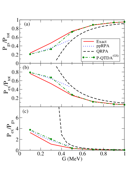
Figure 7: (color online) Ratios of probabilities estimated with different theories for the equidistant level case. The exact (red solid line), QRPA (black dashed line) and P-QTDA (green filled circles) are shown. The ppRPA is also shown (dotted line) up to $G=0.48$ MeV.

To further quantify the predictive power of the P-QTDA^(GS) method, some ratios of pair transfer probabilities are shown in Figure 7. In this figure, $P_{\rm gs}$, $P_{\rm ex}$ and $P_{\rm tot}$ correspond respectively to the probability to transfer to the ground state, the sum of probabilities to transfer to any excited states, while $P_{\rm tot}=P_{\rm gs}+P_{\rm ex}$. Below the pairing threshold, the P-QTDA^(GS) reduces to a ppTDA^(GS), where the diagonalization is made in a reduced space of Slater determinant. In that case, the result are of the same quality as for the ppRPA. This figure clearly confirms that while QRPA is rather far from the exact results in the superfluid phase, especially in the vicinity of the BCS threshold, the projected theory provides a much better reproduction of ground state to excited state pair transfer probabilities. Moreover,theoretical predictions based on the QRPA For02 might significantly overestimate the GPV cross section, as suggested also in Mou11 , especially in the vicinity of the normal-superfluid transition.

V Conclusions

In this work, the QRPA description of the two-particle transfer mechanism is tested against the exact solution in the Richardson model for several conditions of pairing interaction strength and level spacing. It is seen that both ppRPA in the normal phase and QRPA in the superfluid region are able to grasp the gross feature of the pair transfer process. However some differences are observed. At variance with other kind of resonance states mainly build in terms of particle-hole excitations (see for instance Fig. 1 of Ref. Ter08 ) the particle number conservation seems to play an important role when the particle number change during the physical process under interest. A method is proposed here to improve the description of pair transfer in finite superfluid systems. The new method is based on the direct diagonalization of the Hamiltonian in a reduced space of the projected ground state plus two quasi-particle states. This theory improves considerably the description of the pair transfer process. On the practical side, the P-QTDA^(GS) requires only to solve the BCS or HFB problem in the initial nucleus and, except the additional numerical cost of projection, it does not need more effort than the original QRPA. Work is in progress to apply it to nuclear transfer reactions.

- (1) R.A. Broglia, O. Hansen, and C. Riedel, Adv. Nucl. Phys. 6, 287 (1973).
- (2) W. von Oertzen and A.Vitturi, Rep. Prog. Phys. 64, 1247 (2001).
- (3) G. Potel, A. Idini, F. Barranco, E. Vigezzi, R. A. Broglia, nucl-th/0906.4298v3.
- (4) E. Khan, N. Sandulescu, N. V. Giai and M. Grasso, Phys. Rev. C 69, 014314 (2004).
- (5) E. Khan, M. Grasso, and J. Margueron, Phys. Rev. C 80, 044328 (2009).
- (6) B. Avez and C. Simenel, Ph. Chomaz, Phys. Rev. C 78, 044318 (2008).
- (7) B. Mouginot, et al, Phys. Rev. C 83, 037302 (2011).
- (8) J. Dobaczewski, W. Nazarewicz, T. R. Werner, J. F. Berger, C. R. Chinn, and J. Decharg?e, Phys. Rev. C 53, 2809 (1996).
- (9) H. Shimoyama, M. Matsuo, Phys. Rev. C 84, 044317 (2011).
- (10) G. Potel, F. Barranco, F. Marini, A. Idini, E. Vigezzi, and R. A.Broglia, Phys. Rev. Lett. 107, 092501 (2011).
- (11) E. Pllumbi, M. Grasso, D. Beaumel, E. Khan, J. Margueron, and J. van de Wiele Phys. Rev. C 83, 034613 (2011).
- (12) M. Grasso, D. Lacroix, and A. Vitturi, Phys. Rev. C 85, 034317 (2012)
- (13) R. W. Richardson and N. Sherman, Nucl. Phys. 52, 221 (1964); R. W. Richardson, Phys. Rev. 141, 949 (1966); J. Math. Phys. 9, 1327 (1968).
- (14) G. Ripka and R. Padjen, Nucl. Phys. A132, 489 (1969).
- (15) D. R. Bès and R. A. Broglia Nucl. Phys. 80,289 (1966).
- (16) R. A. Broglia and C. Riedel, Nucl. Phys. A107,1 (1968).
- (17) P. Ring and P. Schuck, The Nuclear Many-Body Problem, Springer-Verlag, Berlin, (1980).
- (18) J.-P. Blaizot and G. Ripka, Quantum Theory of Finite Systems (MIT Press, 1986).
- (19) M. Matsuo and Y. Serizawa, Phys. Rev. C 82, 024318 (2010).
- (20) D. M. Brink and R. A. Broglia, Nuclear Superfluidity: Pairing in Finite Systems, Cambridge University Press, Cambridge, England, 2005.
- (21) V. Zelevinsky and A. Volya, Phys. of Atom. Nuclei 66, 1829 (2003).
- (22) D.J. Rowe, Nuclear collective motion: models and theory, World Scientific Publishing Company Incorporated (2010).
- (23) D. Gambacurta, M. Sambataro and F. Catara, Phys. Rev. C73, 014310(2006)
- (24) N . Dinh Dang, Phys. Rev. C74, 024318 (2006)
- (25) N. Quang Hung and N . Dinh Dang, Phys. Rev. C76, 054302 (2007)
- (26) D. Lacroix and D. Gambacurta, Phys. Rev. C 86 014306 (2012).
- (27) M. Kyotoku, K. W. Schmid, F. Grummer, and Amand Faessler Phys. Rev. C 41, 284 (1990).
- (28) K. W. Schmid, M. Kyotoku, F. Grummer and A. Faessler, Annals of Physics 190, 182 (1989).
- (29) C. M. Raduta and A. A. Raduta, Nucl. Phys. A 756, 153 (2005). C. M. Raduta, A. A. Raduta and I. I. Ursu, Phys. Rev. C84, 064322 (2011)
- (30) V. N. Fomenko, J. Phys. G 3, 8 (1970).
- (31) M. Bender, T. Duguet, and D. Lacroix, Phys. Rev. C 79, 044319 (2009).
- (32) N. Sandulescu and G. F. Bertsch, Phys. Rev. C 78, 064318 (2008); N. Sandulescu, B. Errea, and J. Dukelsky, ibid. 80, 044335 (2009).
- (33) G. Hupin and D. Lacroix, Phys. Rev. C 83, 024317 (2011).
- (34) T. R. Rodriguez and J. L. Egido, Phys. Rev. Lett. 99, 062501. (2007).
- (35) T. R. Rodriguez and J. L. Egido, Phys. Rev. C 81, 064323. (2010).
- (36) G. Hupin and D. Lacroix, Phys. Rev. C 86, 024309 (2012).
- (37) J. Terasaki, J. Engel, and G. F. Bertsch, Phys. Rev. C 78, 044311 (2008).
- (38) L. Fortunato, W. von Oertzen, H. M. Sofia and A. Vitturi, Eur. Phys. J. A14, 37 (2002)