Intrinsic and substrate induced spin-orbit interaction in chirally stacked trilayer graphene

Abstract

We present a combined group-theoretical and tight-binding approach to calculate the intrinsic spin-orbit coupling (SOC) in ABC stacked trilayer graphene. We find that compared to monolayer graphene (S. Konschuh, M. Gmitra, and J. Fabian [Phys. Rev. B 82, 245412 (2010)])jfabian-mono-TB , a larger set of $d$ orbitals (in particular the $d_{z^{2}}$ orbital) needs to be taken into account. We also consider the intrinsic SOC in bilayer graphene, because the comparison between our tight-binding bilayer results and the density functional computations of (Ref. jfabian-bilayer, allows us to estimate the values of the trilayer SOC parameters as well. We also discuss the situation when a substrate or adatoms induce strong SOC in only one of the layers of bilayer or ABC trilayer graphene. Both for the case of intrinsic and externally induced SOC we derive effective Hamiltonians which describe the low-energy spin-orbit physics. We find that at the $K$ point of the Brillouin zone the effect of Bychkov-Rashba type SOC is suppressed in bilayer and ABC trilayer graphene compared to monolayer graphene.

I Introduction

The low-energy properties of multilayer graphenegraphene-review depend crucially on the stacking order of the constituent graphene layersmultilayer-guinea ; lu ; luc-hernard ; aoki ; partoens ; rubio ; mccann-abctrilayer ; mccann-abatrilayer ; koshino ; macdonald-1 ; mak ; hung-lui ; nphys-1 ; nphys-2 ; nphys-3 ; nphys-4 . In the case of trilayer graphene, there are two stable stacking orders: (i) ABA or Bernard stacking and (ii) ABC or chiral stacking. Recent advances in sample fabrication methods have resulted in high-quality trilayer samples which can be used to probe many of the theoretical predictionsmak ; hung-lui ; nphys-1 ; nphys-2 ; nphys-3 ; nphys-4 ; khodkov . ABC stacked trilayer graphene appears to be particularly exciting because it is expected to host a wealth of interesting phenomena, such as chiral quasiparticles with Berry phase $3\pi$mccann-abctrilayer , a Lifshitz transition of electronic bands due to trigonal warpingmccann-abctrilayer ; macdonald-1 , band-gap opening in an external electric fieldmultilayer-guinea ; lu ; aoki ; mccann-abctrilayer ; koshino ; macdonald-1 ; avetisyan ; abc-dft-xiao ; nphys-1 ; khodkov , and broken symmetry phases at low electron densitiesmacdonald-2 ; macdonald-3 ; barlas ; cvetkovic , to name a few.

Although there are a number of theoreticalmultilayer-guinea ; aoki ; lu ; luc-hernard ; partoens ; mccann-abctrilayer ; mccann-abatrilayer ; koshino ; rubio ; macdonald-1 ; avetisyan ; abc-dft-xiao ; kumar ; castro and experimentalensslin ; nnanotech ; mak ; kumar ; hung-lui ; nphys-1 ; nphys-2 ; nphys-3 ; nphys-4 studies on the electronic properties of ABA and ABC stacked trilayer graphene, the spin-orbit coupling (SOC) in these systems has received much less attention. ABA trilayer graphene was considered in Ref. mccann-spinorbit, within a framework of an effective low-energy theory, whereas the case ABC stacking was only briefly mentioned in Ref. guinea-so, . The understanding of spin-orbit interaction would be important to study other interesting and experimentally relevant phenomena such as spin relaxationertler ; mccann-monolayerspinorb ; ochoa ; diez , weak-localizationmccann-monolayerspinorb or even spin-Hall effectkane-mele in trilayer graphene. The recent report of Ref. khodkov, on the fabrication of high mobility double gated ABC trilayer graphene may open very promising new avenues for trilayer graphene spintronics as well, similarly to the monolayer case where highly efficient spin transport has recently been reportedfert , but with the additional advantage that external gates can open a band gap in ABC trilayer graphene.

In this paper we aim to make the first steps towards a detailed understanding of the spin-orbit coupling (SOC) in chirally stacked trilayer graphene. We start by investigating the case when the system has inversion symmetry, i.e. in the absence of external electric fields, adatoms or a substrate. This is the case of intrinsic SOC. The intrinsic SOC opens a band-gap at the band-degeneracy points without introducing spin polarization. Previous ab initio calculations on monolayerjfabian-so-numeric ; abdelouahed and bilayerjfabian-bilayer graphene provided strong evidence that the key to the understanding the SOC in flat graphene systems is to take into account the (nominally unoccupied) $d$ orbitals in the description of electronic bands. Here we take the same view and by generalizing the work of Ref. jfabian-mono-TB, derive the intrinsic SOC Hamiltonian for ABC trilayer graphene. It turns out that the most important $d$ orbitals to take into account are the $d_{xz}$, $d_{yz}$ and $d_{z^{2}}$ orbitals. While the former two have been considered in Ref. jfabian-mono-TB, in the context of monolayer graphene, the latter one is important to understand the SOC in AB and ABC graphene. We obtain explicit expressions for the SOC constants in terms of Slater-Kosterslater-koster hopping parameters. We also rederive the intrinsic SO Hamiltonian for bilayer grapheneguinea-so ; jfabian-bilayer . Through the comparison of our trilayer and bilayer analytical results with the recent ab initio calculations of Ref. jfabian-bilayer, we are able to make predictions for the actual values of the SOC parameters in ABC trilayer graphene. The theory involves electronic bands which are far from the Fermi energy $E_{\rm F}$ but are coupled to the physically important low-energy bands close to $E_{\rm F}$ and hence complicate the description of the electronic properties. Therefore, we derive an effective low-energy Hamiltonian and calculate its spectrum. This helps us to understand how SOC lifts certain degeneracies of the electronic bands.

Generally speaking, due to the low atomic number of carbon, the intrinsic SOC in single and multilayer graphene is weak (according to our prediction, the SOC parameters are of the order of $10\,\mu{\rm eV}$ in ABC trilayer, the same as in monolayerboettger ; jfabian-so-numeric ; jfabian-mono-TB ; abdelouahed and bilayerjfabian-bilayer graphene). Recently however, there have been exciting theoretical proposals to enhance the strength of SOC in monolayer graphene and hence, e.g., make the quantum spin Hall statekane-mele observable. These proposals suggest deposition of indium or thallium atomsgraphene-adatom or to bring graphene into proximity with topological insulatorsproximity-spin-orbit . Indeed, very recently the combined experimental and theoretical work of Ref. varykhalov-nature, has provided evidence of a large ($10-100\,{\rm meV}$) spin-orbit gap in monolayer graphene on nickel substrate with intercalated gold atoms. Motivated by these studies we also discuss what might be a minimal model to describe the case where the the SOC is strongly enhanced in only one of the layers of bilayer and ABC trilayer graphene.

Our work is organized as follows. In Sect. II we present the tight-binding (TB) model of ABC-stacked graphene and introduce certain notations that we will be using in subsequent sections. In Sect. III, employing group-theoretical considerations and the Slater-Kosterslater-koster (SK) parametrization of transfer integrals, we derive the SOC Hamiltonian in atomistic approximation at the $K$ point of the Brillouin zone. We repeat this calculation for bilayer graphene in Sect. IV so that in Sect. V we can make predictions for the actual values of the SOC parameters. Next, in Section VI, using $\mathbf{k}\cdotp\mathbf{p}$ theory and the Schrieffer-Wolff transformationwinkler-book ; loss-schrieffer-wolff , we derive an effective low-energy SOC Hamiltonian which is valid for wave-vectors around the $K$ ($K^{\prime}$) point. Finally, in Sect. VII, we consider the case when SOC is enhanced in one of the graphene layers with respect to the other(s).

II Tight-binding model

The basic electronic properties of ABC trilayer are well captured by the effective mass model which is derived assuming one $p_{z}$ type atomic orbital per carbon atom. This model has been discussed in detail in Refs. mccann-abctrilayer, and macdonald-1, ,; therefore we give only a very short introduction here (see also Fig. 1).

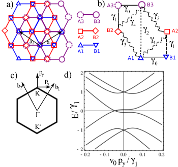
Figure 1: Lattice and band structure of ABC trilayer graphene. a) Lattice structure, where atoms on different layers are indicated with different symbols. $\mathbf{a}_{1}$ and $\mathbf{a}_{2}$ are the two lattice vectors. b) Schematic side view of the unit cell with the most important hopping amplitudes. c) Schematic of the Brillouin zone with reciprocal lattice vectors $\mathbf{b}_{1}$, $\mathbf{b}_{2}$, the high-symmetry points $\Gamma$, $K$ and $K^{\prime}$ and the momentum $\mathbf{p}=(p_{x},p_{y})$ measured from $K$. d) Schematic of the band structure at the $K$ point of the Brillouin zone. The velocity $v_{0}$ is given by $v_{0}=\sqrt{3}/2a\gamma_{0}/\hbar$, where $a$ is the lattice constant: $a=|\mathbf{a}_{1}|$.

There are six carbon atoms in the unit cell of ABC trilayer graphene, usually denoted by $A1$, $B1$, $A2$, $B2$, $A3$, $B3$, where $A$ and $B$ denote the sublattices and $j=1,2,3$ is the layer index. The parameters appearing in the effective model are: $\gamma_{0}$ for the intra-layer $Aj-Bj$ nearest-neighbour hopping, $\gamma_{1}$ for the interlayer hopping between sites $B1-A2$ and $B2-A3$, $\gamma_{3}$ ($\gamma_{4}$) describes weaker nearest-layer hopping between atoms belonging to different (the same) sublattice, and finally $\gamma_{2}$ denotes the direct hopping between sites $A1$ and $B3$ that lie on the same vertical linein the outer layers $1$ and $3$. These hoppings can be obtained by e.g. fitting the numerically calculated band structure with a TB modelrubio ; macdonald-1 . The six $p_{z}$ orbitals in the unit cell give rise to six electronic bandsmccann-abctrilayer ; macdonald-1 . As shown in Fig.1(d), at the $K$ ($K^{\prime}$) point of the Brillouin zone (BZ) two of these bands lie close to the Fermi energy $E_{\rm F}=0$ and we will refer to them as ”low-energy“ states. In addition, there are four ”split-off“ states far from $E_{\rm F}$ at energies $E=\pm\gamma_{1}$.

To obtain the intrinsic SOC Hamiltonian of ABC trilayer graphene we generalize the main idea of Ref. jfabian-mono-TB, where the SOC of monolayer graphene was discussed. Using group-theoretical considerations and density functional theory (DFT) calculations it was shown in Ref. jfabian-mono-TB, that in the case of monolayer graphene the main contribution to the intrinsic SOC comes from the admixture of $p_{z}$ orbitals with some of the (nominally unoccupied) $d$ orbitals, namely, with the $d_{xz}$ and $d_{yz}$ orbitals. The other $d$ orbitals, $d_{z^{2}}$, $d_{xy}$ and $d_{x^{2}-y^{2}}$ play no role due to the fact that they are symmetric with respect to the mirror reflection $\sigma_{h}:(x,y,z)\rightarrow(x,y,-z)$ to the plane of the graphene layer, whereas $p_{z}$ is antisymmetric. The importance of the $d$ orbitals for the understanding of SOC in monolayer graphene was also pointed out in Ref. abdelouahed, .

The symmetry group of ABC stacked trilayer graphene is $R\bar{3}m$ ($D_{3d}$) which does not contain the mirror reflection $\sigma_{h}$. Therefore, from a symmetry point of view, in an approach similar to Ref. jfabian-mono-TB, , all $d$ orbitals need to be taken into account. To derive a TB model one should therefore use as basis set the Bloch wavefunctions

$$\Psi^{\alpha j}_{\beta}(\mathbf{r},\mathbf{k})=\frac{1}{\sqrt{N}}\sum_{n}e^{i\mathbf{k}\cdotp(\mathbf{R}_{n}+\mathbf{t}_{\alpha})}\Phi_{\beta}^{j}(\mathbf{r}-(\mathbf{R}_{n}+\mathbf{t}_{\alpha})),$$ (1)

where the wavevector $\mathbf{k}$ is measured from the $\Gamma$ point of the BZ (see Fig. 1), $\alpha j=\{A1,A2,A3,B1,B2,B3\}$ is a composite index for the sublattice $\alpha=\{A$, $B\}$ and layer $j=\{1,2,3\}$ indices and $\Phi_{\beta}^{j}$ denotes the atomic orbitals of type $\beta=\{p_{z},d_{z^{2}},d_{xz},d_{yz},d_{xy},d_{x^{2}-y^{2}}\}$ in layer $j$. The summation runs over all Bravais lattice vectors $\mathbf{R}_{n}$, whereas the vectors $\mathbf{t}_{\alpha}$ give the position of atom $\alpha$ in the two-dimensional unit cell. We use a coordinate system where the primive lattice vectors are $\mathbf{a}_{1}=\frac{a}{2}(\sqrt{3},1)$ and $\mathbf{a}_{2}=\frac{a}{2}(-\sqrt{3},1)$, the positions of the atoms in the unit cell are $\mathbf{t}_{A1}=\mathbf{t}_{B3}=(0,0)$, $\mathbf{t}_{A2}=\mathbf{t}_{B1}=\frac{a}{2}\left(-\frac{1}{\sqrt{3}},1\right)$ and $\mathbf{t}_{A3}=\mathbf{t}_{B2}=\frac{a}{2}\left(\frac{1}{\sqrt{3}},1\right)$ where $a=2.46\AA{}$ is the lattice constant. The $K$ and $K^{\prime}$ points of the Brillouin zone, which are important for the low energy physics discussed in this paper, can be found at $K=(0,\frac{4\pi}{3a})$, $K^{\prime}=(0,-\frac{4\pi}{3a})$.

The symmetry group of the lattice contains threefold rotations by $\pm{2\pi}/{3}$, about an axis perpendicular to the graphene layers. Since the atomic orbitals $d_{xz},d_{yz},d_{xy},d_{x^{2}-y^{2}}$ themselves do not possess this symmetry, instead of $\Psi^{\alpha j}_{\beta}(\mathbf{r},\mathbf{k})$ given in Eq. (1) we will use Bloch states which depend on $\frac{1}{\sqrt{2}}(d_{xz}\pm id_{yz})\sim\mp Y_{2}^{\pm 1}$, $\frac{1}{\sqrt{2}}(d_{x^{2}-y^{2}}\pm id_{xy})\sim Y_{2}^{\pm 2}$ (rotating orbitals), where $Y_{l}^{m}$ are spherical harmonics. Taking into account that $p_{z}\sim Y_{1}^{0}$ and $d_{z^{2}}\sim Y_{2}^{0}$, the Bloch states we use as basis will be denoted by $\Psi^{\alpha j}_{l,m_{l}}(\mathbf{r},\mathbf{k})$, where $l=1,2$ and $m_{1}=0$, whereas $m_{2}$ can take all allowed values $m_{2}=-2\dots 2$. Often, we will need a linear combination of two of these basis functions where both of the basis functions have the same quantum number $l$ but one of them is centered on an $A$ type atom and the other one is on a $B$ type atom, e.g. $\frac{1}{\sqrt{2}}[\Psi^{A1}_{1,0}(\mathbf{r},\mathbf{k})-\Psi^{B3}_{1,0}(\mathbf{r},\mathbf{k})]$. As a shorthand notation, we will denote the symmetric combination of two such basis functions by $\Psi^{j,j^{\prime}}_{l,m,m^{\prime}}(\mathbf{r},\mathbf{k})=\frac{1}{\sqrt{2}}[\Psi^{Aj}_{l,m}(\mathbf{r},\mathbf{k})+\Psi^{Bj^{\prime}}_{l,m^{\prime}}(\mathbf{r},\mathbf{k})]$ and the antisymmetric one with $\overline{\Psi^{j,j^{\prime}}_{l,m,m^{\prime}}(\mathbf{r},\mathbf{k})}=\frac{1}{\sqrt{2}}[\Psi^{Aj}_{l,m}(\mathbf{r},\mathbf{k})-\Psi^{Bj^{\prime}}_{l,m^{\prime}}(\mathbf{r},\mathbf{k})].$ The first upper index $j$ in $\Psi^{j,j^{\prime}}_{l,m,m^{\prime}}$ always denotes the layer index of the atomic orbital centered on the $A$ type atom, the second upper index $j^{\prime}$ is the layer index for the orbital centered on the $B$ type atom, the first lower index $l$ is the common angular momentum quantum number, and finally, the second and the third lower indices $m$, $m^{\prime}$ give the magnetic quantum number in the same manner as the upper indices give the layer index. To lighten the notation, we will usually suppress the dependence of the Bloch functions on $(\mathbf{r},\mathbf{k})$ and use the bra-ket notation, e.g. $|\Psi^{1,3}_{1,0,0}\rangle$, $|\overline{\Psi^{1,3}_{1,0,0}}\rangle$.

The derivation of the spin-orbit Hamiltonian proceeds in the same spirit as in Ref. jfabian-mono-TB, : (i) First, we neglect the spin degree of freedom. Using the Slater-Koster parametrization to describe the hopping integrals $\langle\Psi^{j,j^{\prime}}_{l,m,m^{\prime}}|\hat{\mathcal{H}}|\Psi^{j^{\prime\prime},j^{\prime\prime\prime}}_{l^{\prime},m^{\prime\prime},m^{\prime\prime\prime}}\rangle$ ($\hat{\mathcal{H}}$ is the single particle Hamiltonian of the system) at a high symmetry point (the $K$ point) of the Brillouin zone and group-theoretical considerations we obtain certain effective Bloch wavefunctions which comprise $p_{z}$ and $d$ atomic orbitals centered on different atoms; (ii) using these effective wavefunctions we calculate the matrix elements of the spin-orbit Hamiltonian in atomic approximation, and (iii) employing the $\mathbf{k}\cdotp\mathbf{p}$ theory we obtain the bands around the $K$ point and then we derive an effective low-energy Hamiltonian.

III Intrinsic SOC

If, in addition to the $p_{z}$ orbitals, we include also the $d$ orbitals into our basis, there will be six basis functions $|\Psi_{l,m}^{\alpha j}\rangle$ centered on each of the six carbon atoms in the unit cell and hence the TB Hamiltonian ${H}_{ABC}$, which is straightforward to calculate in the SK parametrization, is a $36\times 36$ matrix. By e.g. numerically diagonalizing this matrix one would find that the $p_{z}$ orbitals hybridize with some of the $d$ orbitals and one could see how the low energy and the split-off states, obtained in the first instance by neglecting the $d$ orbitals, are modified. According to band theory each state at the $K$ point should belong to one of the irreducible representations of the small group of the $K$ pointdresselhaus-book , which is $32$ ($D_{3}$) in this case. This group has two one-dimensional irreducible representation, denoted by $\Gamma_{A_{1}}$ and $\Gamma_{A_{2}}$ respectively, and a two-dimensional one denoted by $\Gamma_{E}$ (see Appendix A). The matrix elements of ${H}_{ABC}$ between basis states corresponding to different irreducible representations of $D_{3}$ are zerodresselhaus-book . In other words, ${H}_{ABC}$ can be block-diagonalized by choosing suitable linear combinations of the basis functions $|\Psi_{l,m}^{\alpha j}\rangle$ such that the new basis functions transform as the irreducible representations of the group $D_{3}$ because the hybridization between $p_{z}$ and $d$ orbitals will preserve the symmetry properties. A group-theoretical analysis of the problem shows that in a suitable basis ${H}_{ABC}$ is block-diagonal having (i) two $6\times 6$ blocks which we denote by $H_{\Gamma_{A_{1}}}$ and $H_{\Gamma_{A_{2}}}$, they correspond to basis states with $\Gamma_{A_{1}}$ and $\Gamma_{A_{2}}$ symmetry, and (ii) there is one $24\times 24$ block ${H}_{\Gamma_{E}}$ corresponding to states with $\Gamma_{E}$ symmetry. (The basis vectors with $\Gamma_{A_{1}}$, $\Gamma_{A_{2}}$ and $\Gamma_{E}$ symmetries are listed in Appendix A, Table 7). As a concrete example we will consider $H_{\Gamma_{A_{1}}}$ and discuss how one can extract an effective orbital in which $p_{z}$ atomic orbitals with large weight and $d$ orbitals with small weight are admixed. The calculation for $H_{\Gamma_{A_{2}}}$ and ${H}_{\Gamma_{E}}$ cases is analogous and will be presented only briefly.

The basis states transforming as the irreducible representation $\Gamma_{A_{1}}$ are $|\overline{\Psi_{1,0,0}^{1,3}}\rangle$, $|\Psi_{2,1,-1}^{3,1}\rangle$, $|\Psi_{2,0,0}^{1,3}\rangle$, $|\Psi_{2,-2,2}^{3,1}\rangle$, $|\Psi_{2,-1,1}^{2,2}\rangle$ and $|\Psi_{2,2,-2}^{2,2}\rangle$. The TB Hamiltonian $H_{\Gamma_{A_{1}}}$ can be further divided into $3\times 3$ blocks:

$$H_{\Gamma_{A_{1}}}=\left(\begin{array}[]{cc}H_{pd}^{A_{1}}&W^{A_{1}}\\ (W^{A_{1}})^{\dagger}&H_{dd}^{A_{1}}\end{array}\right).$$ (2)

Explicitly, the upper left block $H_{pd}^{A_{1}}$, corresponding to the basis states $|\overline{\Psi_{1,0,0}^{1,3}}\rangle,|\Psi_{2,1,-1}^{3,1}\rangle$ and $|\Psi_{2,0,0}^{1,3}\rangle$, reads

$$H_{pd}^{A_{1}}=\left(\begin{array}[]{ccc}\varepsilon_{p}-\gamma_{2}&\frac{3}{\sqrt{2}}V_{pd\pi}&V_{pd\sigma}^{A1,B3}\\ \frac{3}{\sqrt{2}}V_{pd\pi}&\varepsilon_{d}&0\\ V_{pd\sigma}^{A1,B3}&0&\varepsilon_{d}+V_{dd\sigma}^{A1,B3}\end{array}\right),$$ (6)

where the upper indices $A1$, $B3$ on the SK parameters indicate the atomic sites between which the hopping takes place. The parameter $V_{pd\pi}$ describes hopping between $A$ and $B$ type atoms within the same graphene layer and we assume that its value is the same in all three layers. The matrix elements in $W^{A_{1}}$ of Hamiltonian (2) are either zerozeros or describe skew hoppings between the $p_{z}$ and $d$ orbitals located on different atoms. We assume that these skew hoppings are much smaller than both the vertical hopping $V_{pd\sigma}^{A1,B3}$ and $V_{pd\pi}$. This is not a crucial assumption and the neglected skew-hoppings can be taken into account in a straightforward manner. However, it simplifies the lengthy algebra that follows and we believe it yields qualitatively correct results (see Section IV). With $W^{A_{1}}\approx 0$ we see that $H_{dd}^{A_{1}}$ (corresponding to the basis functions $|\Psi_{2,-2,2}^{3,1}\rangle$, $|\Psi_{2,-1,1}^{2,2}\rangle$ and $|\Psi_{2,2,-2}^{2,2}\rangle$) is decoupled from $H_{pd}$ and that this latter matrix describes the hybridization between the $p_{z}$ orbital based basis vector $|\overline{\Psi_{1,0,0}^{1,3}}\rangle$ and the basis vectors $|\Psi_{2,1,-1}^{3,1}\rangle$, $|\Psi_{2,0,0}^{1,3}\rangle$ involving $d_{xz}$, $d_{yz}$ and $d_{z^{2}}$ orbitals. By diagonalizing $H_{pd}^{A_{1}}$ one could find out how the energy $\varepsilon_{A_{1}}=\varepsilon_{p}-\gamma_{2}$ of one of the low-energy states is modified by the $d$ orbitals. The secular equation $\det(H_{pd}^{A_{1}}-\varepsilon I)=0$ leads to a cubic equation in $\varepsilon$ and the solutions can only be expressed using the Cardano formula. Instead, we next perform a Schrieffer-Wolff transformation (Löwdin partitioning) $\tilde{H}_{pd}^{A_{1}}=e^{-S}\,H_{pd}^{A_{1}}\,e^{S}$ to approximately block-diagonalize $H_{pd}^{A_{1}}$ into a $1\times 1$ and a $2\times 2$ block by eliminating the matrix elements between $|\overline{\Psi_{1,0,0}^{1,3}}\rangle$ on one hand and $|\Psi_{2,1,-1}^{3,1}\rangle$, $|\Psi_{2,0,0}^{1,3}\rangle$ on the other hand. (A detailed discussion of this method can be found in e.g. Refs. winkler-book, ; loss-schrieffer-wolff, .) The matrix $S$ is anti-Hermitian: $S^{\dagger}=-S$ and only its nondiagonal blocks $S_{pd}$ and $-S_{pd}^{\dagger}$ are non-zero. In first orderwinkler-book of the coupling matrix elements $V_{pd\pi}$ and $V_{pd\sigma}^{A1,B3}$ one finds that

$$S^{(1)}_{pd}=-\left(\frac{\bar{V}_{pd\pi}}{\delta\varepsilon_{pd}-\gamma_{2}},\frac{V_{pd\sigma}^{A1,B3}}{\delta\varepsilon_{pd}-\tilde{\gamma}_{2}}\right).$$ (7)

where $\bar{V}_{pd\pi}=\frac{3}{\sqrt{2}}V_{pd\pi}$, $\delta\varepsilon_{pd}=\varepsilon_{p}-\varepsilon_{d}$ and $\tilde{\gamma}_{2}=\gamma_{2}+V_{dd\sigma}^{A1,B3}$. The $1\times 1$ block of $\tilde{H}_{pd}^{A_{1}}$ reads $\tilde{\varepsilon}_{A_{1}}=\varepsilon_{p}-\gamma_{2}+{\bar{V}_{pd\pi}^{2}}/{(\delta\varepsilon_{pd}-\gamma_{2})}+{(V_{pd\sigma}^{A1,B3})^{2}}/{(\delta\varepsilon_{pd}-\tilde{\gamma}_{2})}$, this means that the energy $\varepsilon_{A_{1}}$ of the low energy state is shifted by ${\bar{V}_{pd\pi}^{2}}/{(\delta\varepsilon_{pd}-\gamma_{2})}+{(V_{pd\sigma}^{A1,B3})^{2}}/{(\delta\varepsilon_{pd}-\tilde{\gamma}_{2})}.$ While the Schrieffer-Wolff transformation is usually used to obtain effective Hamiltonians, one can also obtain the new basis in which $\tilde{H}_{pd}^{A_{1}}$ is blockdiagonal. Making the approximation $e^{-S}\approx 1-S$ (see Ref. S-approx, ) we find that the purely $p_{z}$-like state $|\overline{\Psi_{1,0,0}^{1,3}}\rangle$ is transformed into

$$|\Psi_{\Gamma_{A_{1}}}^{p_{z}}\rangle=|\overline{\Psi_{1,0,0}^{1,3}}\rangle+\frac{\bar{V}_{pd\pi}}{\delta\varepsilon_{pd}-\gamma_{2}}|\Psi_{2,1,-1}^{3,1}\rangle+\frac{V_{pd\sigma}^{A1,B3}}{\delta\varepsilon_{pd}-\tilde{\gamma}_{2}}|\Psi_{2,0,0}^{1,3}\rangle,$$ (8)

i.e. it is admixed with two other basis vectors containing $d_{xz},d_{yz}$ and $d_{z^{2}}$ orbitals. Since $|\Psi_{\Gamma_{A_{1}}}^{p_{z}}\rangle$ corresponds to a $1\times 1$ and hence diagonal block of $\tilde{H}_{pd}$, it is an approximate eigenvector of $H_{pd}^{A_{1}}$ with energy $\tilde{\varepsilon}_{A_{1}}$. The upper index $p_{z}$ in $|\Psi_{\Gamma_{A_{1}}}^{p_{z}}\rangle$ is meant to indicate that in this state $p_{z}$ orbitals have the largest weight. There are two other states with $\Gamma_{A_{1}}$ symmetry which could be obtained by diagonalizing the the remaining $2\times 2$ block of $\tilde{H}_{pd}^{A_{1}}$. In these states $|\Psi_{2,1,-1}^{3,1}\rangle$ and $|\Psi_{2,0,0}^{1,3}\rangle$ would have large weight. They are however far remote in energy from $|\Psi_{\Gamma_{A_{1}}}^{p_{z}}\rangle$ and therefore play no role in our further considerations. The situation will be similar in the case of the two other irreducible representations, $\Gamma_{A_{2}}$ and $\Gamma_{E}$, therefore we will suppress the upper index $p_{z}$ henceforth in the notation of the physically important approximate eigenstates.

We now briefly discuss the symmetry classes $\Gamma_{A_{2}}$ and $\Gamma_{E}$. The calculation for the other $6\times 6$ block of $H_{ABC}$ with $\Gamma_{A_{2}}$ symmetry is completely analogous to the $\Gamma_{A_{1}}$ case, the resulting approximate eigenvector, $|\Psi_{\Gamma_{A_{2}}}\rangle$ is shown in the left column of Table 3. Its energy, apart from the shift due to the $d$ orbitals, which will be neglected, is $\varepsilon_{A_{2}}=\varepsilon_{p}+\gamma_{2}$.

The matrix block corresponding to states with $\Gamma_{E}$ symmetry can be written as

$$H_{\Gamma_{E}}=\left(\begin{array}[]{cc}H_{pp}^{E}&W^{E}_{pd}\\ (W^{E}_{pd})^{\dagger}&H_{dd}^{E}\end{array}\right).$$ (9)

Here the $4\times 4$ block $H_{pp}^{E}$ contains the matrix elements between the basis vectors $|{\Psi_{1,0,0}^{2,1}}\rangle$, $|{\Psi_{1,0,0}^{3,2}}\rangle$, $|\overline{\Psi_{1,0,0}^{2,1}}\rangle$, $|\overline{\Psi_{1,0,0}^{3,2}}\rangle$, the $4\times 20$ block $W_{pd}^{E}$ is the coupling matrix between the above shown $p_{z}$ orbital based basis vectors and the $d$ orbitals based basis vectors. (The full set of basis vectors for each of the three symmetry classes is listed in Appendix A.) A direct calculation shows that $H_{pp}$ is a diagonal matrix with $\varepsilon_{p}+\gamma_{1},\varepsilon_{p}+\gamma_{1},\varepsilon_{p}-\gamma_{1},\varepsilon_{p}-\gamma_{1}$ entries. Earlier we have referred to these states as ”split-off“ states. Since $H_{pp}^{E}$ is diagonal, its approximate eigenvectors $|\Psi_{\Gamma_{E_{1,1}}}\rangle$, $|\Psi_{\Gamma_{E_{1,2}}}\rangle$, $|\Psi_{\Gamma_{E_{2,1}}}\rangle$ and $|\Psi_{\Gamma_{E_{2,2}}}\rangle$, which are listed in Table 3, can be obtained in exactly the same way as $|\Psi_{\Gamma_{A_{1}}}\rangle$.

We will refer to the basis formed from the physically important approximate eigenvectors $\{|\Psi_{\Gamma_{A_{1}}}\rangle,|\Psi_{\Gamma_{A_{2}}}\rangle,|\Psi_{\Gamma_{E_{1,1}}}\rangle,|\Psi_{\Gamma_{E_{1,2}}}\rangle,|\Psi_{\Gamma_{E_{2,1}}}\rangle,|\Psi_{\Gamma_{E_{2,2}}}\rangle\}$ as the ”symmetry basis“ henceforth. (The symmetry basis for the $K^{\prime}$ point can be obtained by complex-conjugation.) Looking at these basis vectors we see that in contrast to monolayer graphenejfabian-mono-TB , where only $d_{xz}$ and $d_{yz}$ orbitals hybridize with the $p_{z}$ orbital, here also the $d_{z^{2}}$ orbitals are admixed. As it will be shown below, the admixture of $d_{z^{2}}$ orbitals is crucial to obtain the non-diagonal elements of the SOC Hamiltonian.

We can now proceed to calculate the SOC Hamiltonian. This can be done in the atomic approximation, whereby the spin-orbit interaction is described by the Hamiltonian

$$\hat{H}_{SO}^{atomic}=\frac{\hbar}{4m_{e}^{2}c^{2}}\frac{1}{r}\frac{dV(r)}{dr}\,\mathbf{L}\cdotp\mathbf{S}$$ (10)

Here $V(r)$ is the spherically symmetric atomic potential, $\mathbf{L}$ is the angular momentum operator and $\mathbf{S}=(S_{x},S_{y})$ is a vector of spin Pauli matrices $S_{x},\,S_{y}$ (with eigenvalues $\pm 1$). Introducing the spinful symmetry basis functions by $|\Psi_{\mu}\rangle\rightarrow|\Psi_{\mu}\otimes s\rangle$, where $s=\{\uparrow,\downarrow\}$ denotes the spin degree of freedom and noting that $\mathbf{L}\cdotp\mathbf{S}=L_{z}S_{z}+L_{+}S_{-}+L_{-}S_{+}$, where $L_{\pm}=L_{x}\pm iL_{y}$ and $S_{\pm}=\frac{1}{2}(S_{x}\pm iS_{y})$, it is straightforward to calculate the matrix elements $(H_{so}^{ABC})_{\mu,\nu}=\langle\Psi_{\mu}|\hat{H}_{SO}^{atomic}|\Psi_{\nu}\rangle$ in the symmetry basis introduced earlier. Using the notation $S_{\pm}^{\tau}=\frac{1}{2}(S_{x}\pm i\tau\cdotp S_{y})$, where $\tau=+1\,(-1)$ corresponds to the $K$ ($K^{\prime}$) point of the BZ, the result is shown in Table 1.

SOC	$\Psi_{\Gamma_{A_{1}}}$	$\Psi_{\Gamma_{A_{2}}}$	$\Psi_{\Gamma_{E_{1,1}}}$	$\Psi_{\Gamma_{E_{1,2}}}$	$\Psi_{\Gamma_{E_{2,1}}}$	$\Psi_{\Gamma_{E_{2,2}}}$
$\Psi_{\Gamma_{A_{1}}}$	$0$	$\lambda_{1/2}S_{z}^{\tau}$	$\lambda_{1/3}^{E_{1}}S_{+}^{\tau}$	$\lambda_{1/3}^{E_{1}}S_{-}^{\tau}$	$-\lambda_{1/3}^{E_{2}}S_{+}^{\tau}$	$\lambda_{1/3}^{E_{2}}S_{-}^{\tau}$
$\Psi_{\Gamma_{A_{2}}}$	$\lambda_{1/2}S_{z}$	$0$	$-\lambda_{2/3}^{E_{1}}S_{+}^{\tau}$	$\lambda_{2/3}^{E_{1}}S_{-}^{\tau}$	$\lambda_{2/3}^{E_{2}}S_{+}^{\tau}$	$\lambda_{2/3}^{E_{2}}S_{-}^{\tau}$
$\Psi_{\Gamma_{E_{1,1}}}$	$\lambda_{1/3}^{E_{1}}S_{-}^{\tau}$	$-\lambda_{2/3}^{E_{1}}S_{-}^{\tau}$	$0$	$0$	$\lambda_{3/3}^{z}S_{z}$	$\lambda_{3/3}S_{+}^{\tau}$
$\Psi_{\Gamma_{E_{1,2}}}$	$\lambda_{1/3}^{E_{1}}S_{+}^{\tau}$	$\lambda_{2/3}^{E_{1}}S_{+}^{\tau}$	$0$	$0$	$\lambda_{3/3}S_{-}^{\tau}$	$\lambda_{3/3}^{z}S_{z}$
$\Psi_{\Gamma_{E_{2,1}}}$	$-\lambda_{1/3}^{E_{2}}S_{-}^{\tau}$	$\lambda_{2/3}^{E_{2}}S_{-}^{\tau}$	$\lambda_{3/3}^{z}\,S_{z}$	$\lambda_{3/3}S_{+}^{\tau}$	$0$	$0$
$\Psi_{\Gamma_{E_{2,2}}}$	$\lambda_{1/3}^{E_{2}}S_{+}^{\tau}$	$\lambda_{2/3}^{E_{2}}S_{+}^{\tau}$	$\lambda_{3/3}S_{-}^{\tau}$	$\lambda_{3/3}^{z}S_{z}$	$0$	$0$

Table 1: Intrinsic spin-orbit Hamiltonian $\tau\,H_{so}^{ABC}$ in the symmetry basis. Here $\tau=+1(-1)$ corresponds to the $K$ ($K^{\prime}$) point.

The SOC Hamiltonian shown in Table 1 is the main result of this section. Explicit expressions in terms of SK parameters for the coupling constants appearing in Table 1 can be found in Table 3. In contrast to previous works where SOC in ABC trilayer was discussedkonschuh-phd ; guinea-so , we find that the number of SOC parameters is seventwo-soc-param . As we will show, $\lambda_{1/3}^{E_{1}},\lambda_{1/3}^{E_{2}},\lambda_{2/3}^{E_{1}}$ and $\lambda_{2/3}^{E_{2}}$ are related to interlayer SOC and calculations which are based on the symmetry properties of low-energy effective Hamiltonians may not capture them. The $\lambda_{3/3}$ parameter ensures that the otherwise fourfold degeneracy of the split-off states at the $K$ point is lifted, as it is dictated by general group-theoretical considerationsdresselhaus-paper ; dresselhaus-book . These five parameters are proportional to the product $V_{pd\pi}V_{pd\sigma}$ and they could not be obtained considering only the $d_{xz}$, $d_{yz}$ orbitals and in-plane SOC. The remaining two SOC parameters, $\lambda_{1/2}$ and $\lambda_{3/3}^{z}$ are proportional to $V_{pd\pi}^{2}$ and describe in-plane SOC.

SOC	$\Psi^{A1}_{\rm eff}$	$\Psi^{B3}_{\rm eff}$	$\Psi^{B1}_{\rm eff}$	$\Psi^{A2}_{\rm eff}$	$\Psi^{B2}_{\rm eff}$	$\Psi^{A3}_{\rm eff}$
$\Psi^{A1}_{\rm eff}$	${\lambda}_{1/2}\,S_{z}$	$0$	${\lambda}_{2}\,S_{+}^{\tau}$	$\lambda_{1}\,S_{+}^{\tau}$	$\lambda_{4}\,S_{-}^{\tau}$	$\lambda_{3}\,S_{-}^{\tau}$
$\Psi^{B3}_{\rm eff}$	$0$	$-\lambda_{1/2}\,S_{z}$	$-\lambda_{3}\,S_{+}^{\tau}$	$-\lambda_{4}\,S_{+}^{\tau}$	$-\lambda_{1}\,S_{-}^{\tau}$	$-\lambda_{2}\,S_{-}^{\tau}$
$\Psi^{B1}_{\rm eff}$	${\lambda}_{2}\,S_{-}^{\tau}$	$-\lambda_{3}\,S_{-}^{\tau}$	$-{\lambda}_{3/3}^{z}\,S_{z}$	$0$	$-\lambda_{3/3}\,S_{+}^{\tau}$	$0$
$\Psi^{A2}_{\rm eff}$	$\lambda_{1}\,S_{-}^{\tau}$	$-\lambda_{4}\,S_{-}^{\tau}$	$0$	$\lambda_{3/3}^{z}\,S_{z}$	$0$	$\lambda_{3/3}\,S_{+}^{\tau}$
$\Psi^{B2}_{\rm eff}$	$\lambda_{4}\,S_{+}^{\tau}$	$-\lambda_{1}\,S_{+}^{\tau}$	$-\lambda_{3/3}\,S_{-}^{\tau}$	$0$	$-\lambda_{3/3}^{z}\,S_{z}$	$0$
$\Psi^{A3}_{\rm eff}$	$\lambda_{3}\,S_{+}^{\tau}$	$-\lambda_{2}\,S_{+}^{\tau}$	$0$	$\lambda_{3/3}\,S_{-}^{\tau}$	$0$	$\lambda_{3/3}^{z}\,S_{z}$

Table 2: $\tau\,H_{so}^{ABC}$ in the basis of effective $p_{z}$ orbitals.

$|\Psi_{\Gamma_{A_{1}}}\rangle=|\overline{\Psi_{1,0,0}^{1,3}}\rangle+\frac{3}{\sqrt{2}}\frac{V_{pd\pi}}{\delta\varepsilon_{pd}-\gamma_{2}}|\Psi_{2,1,-1}^{3,1}\rangle+\frac{\tilde{V}_{pd\sigma}}{\delta\varepsilon_{pd}-\tilde{\gamma}_{2}}|\Psi_{2,0,0}^{1,3}\rangle$	$\lambda_{1/2}=-\frac{9}{2}\,\xi_{d}\,\frac{(V_{pd\pi})^{2}}{(\delta\varepsilon_{pd}+\gamma_{2})(\delta\varepsilon_{pd}-\gamma_{2})}$
$|\Psi_{\Gamma_{A_{2}}}\rangle=|\Psi_{1,0,0}^{1,3}\rangle-\frac{3}{\sqrt{2}}\frac{V_{pd\pi}}{\delta\varepsilon_{pd}+\gamma_{2}}|\overline{\Psi_{2,1,-1}^{3,1}}\rangle-\frac{\tilde{V}_{pd\sigma}}{\delta\varepsilon_{pd}+\tilde{\gamma}_{2}}|\overline{\Psi_{2,0,0}^{1,3}}\rangle$	$\lambda_{1/3}^{E_{1}}=\frac{3\sqrt{3}}{2}\,\xi_{d}\,\frac{V_{pd\pi}}{(\delta\varepsilon_{pd}+\gamma_{1})}\left(\frac{\tilde{V}_{pd\sigma}}{\delta\varepsilon_{pd}-\tilde{\gamma}_{2}}-\frac{V_{pd\sigma}}{\delta\varepsilon_{pd}-\gamma_{2}}\right)$
$|\Psi_{\Gamma_{E_{1,1}}}\rangle=|\Psi_{1,0,0}^{2,1}\rangle+\frac{1}{\delta\varepsilon_{pd}+\gamma_{1}}\left[\frac{V_{pd\sigma}}{\sqrt{2}}|\overline{\Psi_{2,0,0}^{2,1}}\rangle-\frac{3V_{pd\pi}}{2}|\overline{\Psi_{2,1,-1}^{1,2}}\rangle\right]$	$\lambda_{1/3}^{E_{2}}=\frac{3\sqrt{3}}{2}\,\xi_{d}\,\frac{V_{pd\pi}}{(\delta\varepsilon_{pd}-\gamma_{1})}\left(\frac{\tilde{V}_{pd\sigma}}{\delta\varepsilon_{pd}-\tilde{\gamma}_{2}}+\frac{V_{pd\sigma}}{\delta\varepsilon_{pd}-\gamma_{2}}\right)$
$|\Psi_{\Gamma_{E_{1,2}}}\rangle=|\Psi_{1,0,0}^{3,2}\rangle+\frac{1}{\delta\varepsilon_{pd}+\gamma_{1}}\left[\frac{V_{pd\sigma}}{\sqrt{2}}|\overline{\Psi_{2,0,0}^{3,2}}\rangle-\frac{3V_{pd\pi}}{2}|\overline{\Psi_{2,1,-1}^{2,3}}\rangle\right]$	$\lambda_{2/3}^{E_{1}}=\frac{3\sqrt{3}}{2}\,\xi_{d}\,\frac{V_{pd\pi}}{(\delta\varepsilon_{pd}+\gamma_{1})}\left(\frac{\tilde{V}_{pd\sigma}}{\delta\varepsilon_{pd}+\tilde{\gamma}_{2}}+\frac{V_{pd\sigma}}{\delta\varepsilon_{pd}+\gamma_{2}}\right)$
$|\Psi_{\Gamma_{E_{2,1}}}\rangle=|\overline{\Psi_{1,0,0}^{2,1}}\rangle+\frac{1}{\delta\varepsilon_{pd}-\gamma_{1}}\left[\frac{3V_{pd\pi}}{2}|\Psi_{2,1,-1}^{1,2}\rangle-\frac{V_{pd\sigma}}{\sqrt{2}}|\Psi_{2,0,0}^{2,1}\rangle\right]$	$\lambda_{2/3}^{E_{2}}=\frac{3\sqrt{3}}{2}\,\xi_{d}\,\frac{V_{pd\pi}}{(\delta\varepsilon_{pd}-\gamma_{1})}\left(\frac{\tilde{V}_{pd\sigma}}{\delta\varepsilon_{pd}+\tilde{\gamma}_{2}}-\frac{V_{pd\sigma}}{\delta\varepsilon_{pd}+\gamma_{2}}\right)$
$|\Psi_{\Gamma_{E_{2,2}}}\rangle=|\overline{\Psi_{1,0,0}^{3,2}}\rangle+\frac{1}{\delta\varepsilon_{pd}-\gamma_{1}}\left[\frac{3V_{pd\pi}}{2}|\Psi_{2,1,-1}^{2,3}\rangle-\frac{V_{pd\sigma}}{\sqrt{2}}|\Psi_{2,0,0}^{3,2}\rangle\right]$	$\lambda_{3/3}={3\sqrt{3}}\,\xi_{d}\,\frac{V_{pd\pi}V_{pd\sigma}}{(\delta\varepsilon_{pd}+\gamma_{1})(\delta\varepsilon_{pd}-\gamma_{1})}$
	$\lambda_{3/3}^{z}=-\frac{9}{2}\,\xi_{d}\,\frac{(V_{pd\pi})^{2}}{(\delta\varepsilon_{pd}+\gamma_{1})(\delta\varepsilon_{pd}-\gamma_{1})}$

Table 3: Symmetry basis functions (left column) and intrinsic spin-orbit matrix elements (right column) in terms of Slater-Koster parameters. Here $\xi_{d}$ is the angular momentum resolved atomic SOC strength, $V_{dd\sigma}=V_{dd\sigma}^{A1,B3}$, $\tilde{V}_{pd\sigma}=V_{pd\sigma}^{A1,B3}$, $V_{pd\sigma}=V_{pd\sigma}^{A2,B1}=V_{pd\sigma}^{A3,B2}$, $\delta\varepsilon_{pd}=\varepsilon_{p}-\varepsilon_{d}$, $\tilde{\gamma}_{2}=\gamma_{2}+V_{dd\sigma}$ and we assumed that $V_{pd\pi}=V_{pd\pi}^{Ai,Bi}$, $i=1,2,3$. Although the basis functions shown in the right are not normalized, the SOC parameters are correct in the lowest order of the products of the small parameters ${\tilde{V}_{pd\sigma}}/{(\delta\varepsilon_{pd}\pm\tilde{\gamma}_{2})}$, ${{V}_{pd\sigma}}/{(\delta\varepsilon_{pd}\pm{\gamma}_{2})}$, ${V_{pd\pi}}/{(\delta\varepsilon_{pd}\pm\gamma_{1})}$

The physical meaning of these SOC parameters is probably more transparent if one rotates $H_{so}^{ABC}$ into the basis of on-site effective $p_{z}$ orbitals (see Appendix B.1) . These basis vectors result from the admixture of an on-site $p_{z}$ orbital $|\Psi_{1,0}^{\alpha j}\rangle$ with large weight and $|\Psi_{2,\pm 1}^{\alpha^{\prime}j}\rangle$, $|\Psi_{2,0}^{\alpha j}\rangle$ ($\alpha\neq\alpha^{\prime}$) with small weight. $H_{so}^{ABC}$ in the on-site effective $p_{z}$ basis is shown in Table 2. The SOC parameters $\lambda_{1},\lambda_{2},\lambda_{3}$ and $\lambda_{4}$ are linear combinations of $\lambda_{1/3}^{E_{1}}$, $\lambda_{1/3}^{E_{2}}$, $\lambda_{2/3}^{E_{1}}$ and $\lambda_{2/3}^{E_{2}}$, the explicit relations are given in Section V. In Section V we will also make predictions which might be useful to guide the fitting procedure if results of DFT calculations are fitted with a TB model, as e.g. in Ref. jfabian-bilayer, .

Since the lattice of Bernard stacked bilayer graphene has the same symmetry group as ABC trilayer, the considerations made in this section can be easily applied to bilayer graphene as well. A brief summary of the bilayer calculations is given in Section IV. The importance of the bilayer results is that they can be compared with the numerical calculations of Ref. jfabian-bilayer, . Based on this comparison we will be able to estimate the values of five of the seven SOC parameters of ABC trilayer.

IV Intrinsic SOC in bilayer graphene

In this Section we give a brief summary of our TB calculations for the intrinsic SOC in bilayer graphene and compare the results to the DFT computations of Ref. jfabian-bilayer, . The low-energy states of bilayer are also found at the $K$ and $K^{\prime}$ points of the BZ, hence the calculation follows the same steps as in Section III: (i) first we obtain the basis states of the symmetry basis $\{|\Psi_{\Gamma_{A_{1}}}\rangle,|\Psi_{\Gamma_{A_{2}}}\rangle,|\Psi_{\Gamma_{E_{1,1}}}\rangle,|\Psi_{\Gamma_{E_{1,2}}}\rangle\},$ and (ii) we calculate the matrix elements of $\hat{H}_{SO}^{atomic}$. Note that in the case of bilayer graphene there is only one pair of bands which transforms as the two-dimensional representation $\Gamma_{E}$.

For easier comparison we adopt the notation of Ref. jfabian-bilayer, for the SOC parameters. As it is shown in Table 4, the SO Hamiltonian in the basis of the effective $p_{z}$ orbitals can be written in a form which, apart from a unitary transformation, agrees with the result given in Table IV of Ref. jfabian-bilayer, (see Appendix A for details).

SOC	$\Psi^{A1}_{\rm eff}$	$\Psi^{B1}_{\rm eff}$	$\Psi^{A2}_{\rm eff}$	$\Psi^{B2}_{\rm eff}$
$\Psi^{A1}_{\rm eff}$	${\lambda}_{\rm I2}\,S_{z}$	$\lambda_{0}\,S_{-}^{\tau}$	${\lambda}_{4}^{bi}\,S_{+}^{\tau}$	$0$
$\Psi^{B1}_{\rm eff}$	$\lambda_{0}\,S_{+}^{\tau}$	$-\lambda_{\rm I1}\,S_{z}$	$0$	$-\lambda_{4}^{bi}\,S_{+}^{\tau}$
$\Psi^{A2}_{\rm eff}$	${\lambda}_{4}^{bi}\,S_{-}^{\tau}$	$0$	${\lambda}_{\rm I1}\,S_{z}$	$-\lambda_{0}\,S_{-}^{\tau}$
$\Psi^{B2}_{\rm eff}$	$0$	$-\lambda_{4}^{bi}\,S_{-}^{\tau}$	$-\lambda_{0}\,S_{+}^{\tau}$	$-\lambda_{\rm I2}\,S_{z}$

Table 4: Intrinsic spin-orbit Hamiltonian $\tau\,H_{so}^{AB}$ of bilayer graphene in the basis of effective $p_{z}$ orbitals.

In terms of the SK hoppings, the SOC parameters read:

$$\lambda_{0} = 3\sqrt{3}\,\xi_{d}\,\frac{V_{pd\pi}V_{pd\sigma}}{\delta\varepsilon_{pd}^{2}-\tilde{\gamma}_{1}^{2}}\frac{\tilde{\gamma}_{1}}{\varepsilon_{pd}};\hskip 20.00003pt\lambda_{\rm I1}=\frac{9}{2}\,\xi_{d}\,\frac{V_{pd\pi}^{2}}{\delta\varepsilon_{pd}^{2}};$$

$$\lambda_{4}^{bi} = 3\sqrt{3}\,\xi_{d}\,\frac{V_{pd\pi}V_{pd\sigma}}{\delta\varepsilon_{pd}^{2}-\tilde{\gamma}_{1}^{2}};\hskip 20.00003pt\lambda_{\rm I2}=\frac{9}{2}\,\xi_{d}\,\frac{V_{pd\pi}^{2}}{\delta\varepsilon_{pd}^{2}-\gamma_{1}^{2}}$$ (11)

where $\tilde{\gamma}_{1}=\gamma_{1}+V_{dd\sigma}$. Looking at the expressions given in (11), one can make the following observations: (i) Since $\delta\varepsilon_{pd}=\varepsilon_{p}-\varepsilon_{d}<0$ and $\tilde{\gamma}_{1}>0$, one can expect that the sign of $\lambda_{0}$ and $\lambda_{4}^{bi}$ will be different; (ii) $|\lambda_{0}|<|\lambda_{4}^{bi}|$ because $\frac{\tilde{\gamma}_{1}}{|\varepsilon_{pd}|}<1$; (iii) $\lambda_{\rm I1}$ and $\lambda_{\rm I2}$ have the same sign and they are approximately of the same magnitude because $\gamma_{1}^{2}/\delta\varepsilon_{pd}^{2}\ll 1$.

By fitting the band structure obtained from DFT calculations with their tight binding model, the authors of Ref. jfabian-bilayer, found the following values for the bilayer SOC parameters: $2\lambda_{\rm I1}=24\mu{\rm eV}$, $2\lambda_{\rm I2}=20\mu{\rm eV}$, $\lambda_{0}=5\mu{\rm eV}$, $\lambda_{4}=-12\mu{\rm eV}$. These numbers are in qualitative agreement with the predictions that we made below Eq. (11) for the SOC parameters. If, in addition, one assumes that $V_{pd\pi}V_{pd\sigma}<0$ then according to (11) three of the parameters ($\lambda_{\rm I1}$, $\lambda_{\rm I2}$, $\lambda_{0}$) should have the same sign, which would again agree with the results of Ref. jfabian-bilayer, .

V SOC parameters for trilayer graphene in terms of SK hoppings

We are now ready to make predictions for five of the seven ABC trilayer SOC parameters. To this end, we first express the SOC parameters in the effective $p_{z}$ orbital basis in terms of the SOC parameters obtained in the symmetry basis. Moreover, using the formulae given in Table 3 for $\lambda_{1/3}^{E_{1}}$, $\lambda_{1/3}^{E_{2}}$, $\lambda_{2/3}^{E_{1}}$ and $\lambda_{2/3}^{E_{2}}$, one can also express $\lambda_{1}$, $\lambda_{2}$, $\lambda_{3}$ and $\lambda_{4}$ in terms of the SK hoppings. Taking into account the results of the previous section, this then facilitates making predictions for the numerical values of the ABC trilayer SOC parameters.

First, the SOC parameters in terms of the SK hoppings:

$$\lambda_{1} = (\lambda_{1/3}^{E_{1}}+\lambda_{2/3}^{E_{2}}-\lambda_{1/3}^{E_{2}}-\lambda_{2/3}^{E_{1}})/2$$ (12a)

$$\approx \eta\left(-V_{pd\sigma}+\tilde{V}_{pd\sigma}\frac{\gamma_{2}}{\delta\varepsilon_{pd}}\right),$$

$$\lambda_{2} = (\lambda_{1/3}^{E_{1}}+\lambda_{1/3}^{E_{2}}-\lambda_{2/3}^{E_{1}}-\lambda_{2/3}^{E_{2}})/2$$ (12b)

$$\approx \eta\left(V_{pd\sigma}\frac{\gamma_{1}}{\delta\varepsilon_{pd}}+\tilde{V}_{pd\sigma}\frac{\gamma_{2}}{\delta\varepsilon_{pd}}\right),$$

$$\lambda_{3} = (\lambda_{1/3}^{E_{1}}+\lambda_{1/3}^{E_{2}}+\lambda_{2/3}^{E_{1}}+\lambda_{2/3}^{E_{2}})/2$$ (12c)

$$\approx \eta\left(V_{pd\sigma}\frac{\gamma_{1}}{\delta\varepsilon_{pd}}\frac{\gamma_{2}}{\delta\varepsilon_{pd}}+\tilde{V}_{pd\sigma}\right),$$

$$\lambda_{4} = (\lambda_{1/3}^{E_{1}}+\lambda_{1/3}^{E_{2}}+\lambda_{2/3}^{E_{1}}+\lambda_{2/3}^{E_{2}})/2$$ (12d)

$$\approx \eta\left(V_{pd\sigma}\frac{\gamma_{2}}{\delta\varepsilon_{pd}}+\tilde{V}_{pd\sigma}\frac{\gamma_{1}}{\delta\varepsilon_{pd}}\right),$$

where $\eta=3\sqrt{3}\,\xi_{d}\,\frac{V_{pd\pi}}{\delta\varepsilon_{pd}^{2}-\gamma_{1}^{2}}$. Similarly to the bilayer case, looking at Table 3 and Eqs. (12) one can make the following observations: (i) One would expect that $\lambda_{1/2}\approx\lambda_{3/3}^{z}$, (ii) $|\lambda_{3/3}|\approx|\lambda_{1}|$ and assuming that $V_{pd\sigma}/\tilde{V}_{pd\sigma}\propto\gamma_{1}/\gamma_{2}$ one finds that $|\lambda_{1}|>|\lambda_{2}|>|\lambda_{3}|>|\lambda_{4}|$, and (iii) $\lambda_{4}$ has opposite sign from $\lambda_{3}$ and similarly for $\lambda_{3/3}$ and $\lambda_{1}$ because the second term in the expression for $\lambda_{1}$ in Eq. (12a) can be neglected with respect to the first one.

Comparing the expressions in terms of the SK hoppings given in Eqs. (12) with the corresponding ones for the bilayer case in (11), the following estimates can be made: $2\lambda_{1/2}^{z}\approx 2\lambda_{3/3}^{z}\approx 20\mu{\rm eV}$, $|\lambda_{3/3}|\approx|\lambda_{1}|\approx 10\mu{\rm eV}$ and $|\lambda_{2}|\approx 5\mu{\rm eV}$. Since $\lambda_{3}$ and $\lambda_{4}$ are proportional to $\tilde{V}_{pd\sigma}$ (assuming $V_{pd\sigma}/\tilde{V}_{pd\sigma}\propto\gamma_{1}/\gamma_{2}$) which is unknown, we cannot give a numerical estimate for their value. One would expect that they are much smaller than $\lambda_{1}$ and $\lambda_{2}$ because $\tilde{V}_{pd\sigma}$ corresponds to a remote, and presumably weak $p-d$ hopping between the $A1$ and $B3$ sites.

VI Effective SOC Hamiltonian

The calculations in the previous sections are valid, strictly speaking, only at the $K$ point of the Brillouin zone. To obtain the Hamiltonian in the vicinity of the $K$ point, where the states close to the Fermi energy can be found, one can perform a $\mathbf{k}\cdotp\mathbf{p}$ expansion of the bands. We neglect the weak $\mathbf{k}$ dependence of the SOC jfabian-bilayer , hence the total Hamiltonian of the system can be written as $\hat{H}_{ABC}=\hat{H}_{\mathbf{k}\cdotp\mathbf{p}}^{ABC}+\tau\,\hat{H}_{so}^{ABC}$. Here ${\hat{H}}_{\mathbf{k}\cdotp\mathbf{p}}^{ABC}$ is the $\mathbf{k}\cdotp\mathbf{p}$ Hamiltonian obtained without taking into account the SOC, whereas ${\hat{H}}_{so}^{ABC}$ is the SOC Hamiltonian calculated at the $K$ point. ${\hat{H}}_{\mathbf{k}\cdotp\mathbf{p}}^{ABC}$ has been published before, see e.g. Refs. mccann-abctrilayer, ; macdonald-1, .

To study the low energy physics however, in which we are primarily interested, the use of ${\hat{H}}_{\mathbf{k}\cdotp\mathbf{p}}^{ABC}$ is not convenient, since it includes four bands that are split-off from the Fermi energy of the (undoped) ABC trilayer by the large energy scale $\approx\pm\gamma_{1}$mccann-abctrilayer ; macdonald-1 . Therefore we derive an effective two component (or, including the spin, four component) Hamiltonian $\hat{H}^{\rm eff}_{ABC}$ which describes the hopping between atomic sites $A1$ and $B3$. To this end we again employ the Schrieffer-Wolff transformation and keep all terms which are third order or less in the momentum $\pi$, $\pi^{\dagger}$ and first order in the SOC constants. Here $\pi=-(ip_{x}+\tau p_{y})$, where $\tau=1(-1)$ for valley $K$ ($K^{\prime}$) and the momenta $p_{x},p_{y}$ are measured from the $K$ ($K^{\prime}$) point of the BZ, see Fig. 1(c). Keeping terms up to third order in $\pi$, $\pi^{\dagger}$ is essential to reproduce the important features of the low-energy band structuremccann-abctrilayer ; macdonald-1 , such as the band degeneracy and the trigonal warping. The necessary formulae for the matrix elements of the effective Hamiltonian can be found in Ref. winkler-book, . We treat $\gamma_{1}$ as a large energy scale with respect to $v_{0}\pi$, $|\gamma_{3}|$, $\gamma_{4}$, $\gamma_{2}$ and the typical energies $E$ we are interested in and keep only the leading order for the terms involving $\gamma_{2}$, $v_{3}$ and $v_{4}$. (The velocities $v_{i}$ are given by $v_{i}=(\sqrt{3}/2)a\gamma_{i}/\hbar$, where $a=0.246\,{\rm nm}$ is the lattice constant of graphene.) For the folding down of the full Hamiltonian we use the form of $\hat{H}_{ABC}$ in the symmetry basis because in this case all the large matrix elements are on the diagonal and therefore the quasidegenerate perturbation approach is expected to work well. Once we obtain the effective Hamiltonian $\hat{H}^{\rm eff}_{ABC}$ in the symmetry basis we rotate it into the basis of effective $p_{z}$ orbitals centered on atomic sites $A1$ and $B3$ because $\hat{H}^{\rm eff}$ assumes a simpler form in this basis. Explicitly, one can write $\hat{H}^{\rm eff}_{ABC}=\hat{H}^{\rm eff}_{el}+\hat{H}^{\rm eff}_{so}$, where the electronic part is given by

$${\hat{H}}^{\rm\,eff}_{el} = {\hat{H}}_{chir}+{\hat{H}}_{3w}+\hat{H}_{\gamma_{2}}+{\hat{H}}_{v_{4}},$$

$${\hat{H}}_{chir} = \frac{v_{0}^{3}}{\gamma_{1}^{2}}\left(\begin{array}[]{cc}0&\left({\pi}^{{\dagger}}\right)^{3}\\ {\pi^{3}}&0\end{array}\right),$$ (13c)

$${\hat{H}}_{3w} = -\frac{v_{0}v_{3}}{\gamma_{1}}[\pi^{\dagger}\pi+\pi\pi^{\dagger}]\left(\begin{array}[]{cc}0&1\\ 1&0\end{array}\right),$$ (13f)

$$\hat{H}_{\gamma_{2}} = \gamma_{2}\left(1-\frac{1}{2}\frac{v_{0}^{2}}{\gamma_{1}^{2}}[\pi^{\dagger}\pi+\pi\pi^{\dagger}]\right)\left(\begin{array}[]{cc}0&1\\ 1&0\end{array}\right),$$ (13i)

$${\hat{H}}_{v_{4}} = -\frac{2v_{0}v_{4}}{\gamma_{1}}\left(\begin{array}[]{cc}\pi^{\dagger}\pi&0\\ 0&\pi\pi^{\dagger}\end{array}\right).$$ (13l)

We note that when applying the Schrieffer-Wolff transformation we did not assume that $\pi$ and $\pi^{\dagger}$ commute, therefore the Hamiltonians (13) and (14f) are valid in the presence of finite external magnetic field as well. In zero magnetic field, using the notation $p^{2}=\pi\pi^{\dagger}=\pi^{\dagger}\pi$, the Hamiltonian (13) simplifies to the corresponding results in Refs. mccann-abctrilayer, ; macdonald-1, .

The effective SOC Hamiltonian is

$${\hat{H}}^{\rm\,eff}_{so} = {\hat{H}}_{so}^{mn}+{\hat{H}}_{so}^{(1)}+{\hat{H}}_{so}^{(2)}+{\hat{H}}_{so}^{(3)},$$

$${\hat{H}}_{so}^{mn} = \tau\,\lambda_{1/2}S_{z}\sigma_{z},$$ (14a)

$${\hat{H}}_{so}^{(1)} = -\tau\,\tilde{\lambda}_{1}\,\frac{v_{0}}{\gamma_{1}}\,[S_{-}^{\tau}\pi^{\dagger}+S_{+}^{\tau}\pi]\sigma_{z},$$ (14b)

$${\hat{H}}_{so}^{(2)} = \tau\,\frac{v_{0}v_{3}}{\gamma_{1}^{2}}\lambda_{3/3}[S_{+}^{\tau}(\pi^{\dagger})^{2}+S_{-}^{\tau}\pi^{2}]\sigma_{z},$$ (14c)

$${\hat{H}}_{so}^{(3)} = -\tau\,\frac{v_{0}^{2}}{\gamma_{1}^{2}}(\lambda_{3/3}^{z}-\lambda_{1/2})S_{z}\left(\begin{array}[]{cc}\pi^{\dagger}\pi&0\\ 0&-\pi\pi^{\dagger}\end{array}\right).$$ (14f)

Here the Pauli matrix $\sigma_{z}$ acts in the space of $\{A1,B3\}$ sites and $\tilde{\lambda}_{1}=\lambda_{1}+\lambda_{3}(v_{3}/v_{0})+\lambda_{2}(v_{4}/v_{0})\approx\lambda_{1}$. At low energies $v_{0}^{2}p^{2},v_{0}v_{3}p^{2}\ll\gamma_{1}^{2}$ and the corresponding terms in (14f) can be neglected. The first term, ${\hat{H}}_{so}^{mn}$ is the well known SO Hamiltonian of monolayer graphenekane-mele and describes the leading contribution to SOC. The next term, ${\hat{H}}_{so}^{(1)}$ is the most important momentum dependent contribution close to the $K$ point. Keeping only ${\hat{H}}_{so}^{(mn)}$ and ${\hat{H}}_{so}^{(1)}$ the effective SOC Hamiltonian can be written in a more compact form as

$${\hat{H}}^{\rm\,eff}_{so}=\tau\,\left[\lambda_{1/2}S_{z}+\tilde{\lambda}_{1}\frac{v_{0}}{\gamma_{1}}\left(\mathbf{S}\times\mathbf{p}\right)_{z}\right]\sigma_{z},$$ (15)

where $\mathbf{p}=(p_{x},p_{y})$. We note that Eq. (15) also describes the effective SOC Hamiltonian of bilayer graphene with $\lambda_{1/2}$ replaced by $-\lambda_{\rm I1}$ and $\tilde{\lambda}_{1}=-\lambda_{4}^{bi}+\lambda_{0}(v_{4}/v_{0})\approx-\lambda_{4}^{bi}$ (for $\lambda_{\rm I1}$, $\lambda_{0}$ and $\lambda_{4}^{bi}$ see Sect. IV).

In zero external magnetic field $\hat{H}^{\rm eff}_{ABC}$ is easily diagonalizable. Keeping only the leading terms (15) in $\hat{H}^{\rm\,eff}_{so}$, we obtain the eigenvalues $E_{\pm}=-2\frac{v_{0}v_{4}}{\gamma_{1}}p^{2}\pm r(\mathbf{p})$ (each doubly degenerate) where $r(\mathbf{p})=\sqrt{\lambda_{1/2}^{2}+|c(\mathbf{p})|^{2}+|d(\mathbf{p})}|^{2}$, $c(\mathbf{p})=-\tilde{\lambda}_{1}\frac{v_{0}}{\gamma_{1}}pe^{i\phi_{\mathbf{p}}}$, $d(\mathbf{p})=\gamma_{2}-\frac{2v_{0}v_{3}}{\gamma_{1}}p^{2}+\frac{v_{0}^{3}}{\gamma_{1}^{2}}p^{3}e^{-3i\phi_{\mathbf{p}}}$ where $p=|\pi|$) whereas $\phi_{\mathbf{p}}$ is the phase of $\pi$. The main effect of SOC on the spectrum is, similarly to monolayerkane-mele and bilayerguinea-so ; jfabian-bilayer graphene, to open a band gap $E_{bg}=2\sqrt{\lambda_{1/2}^{2}+|c(\mathbf{p}_{d})|^{2}}$ at the band degeneracy points $\mathbf{p}_{d}$, while preserving the spin degeneracy of the bands (see Fig. 2). Comparing $E_{bg}$ to the SOC band gap in monolayer and bilayer graphene at the $K$ point, we expect that in ABC trilayer it should be somewhat bigger due to the $|c(\mathbf{p}_{d})|^{2}$ term, i.e. because the band gap can be found away from the $K$ point at finite $\mathbf{p}_{d}$. In Fig. 2 we compare the low-energy bands calculated using the full Hamiltonian (which includes the high-energy bands as well) and using the effective Hamiltonian $\hat{H}^{\rm eff}_{ABC}$ .From this, we conclude that the effective theory represents a good approximation.

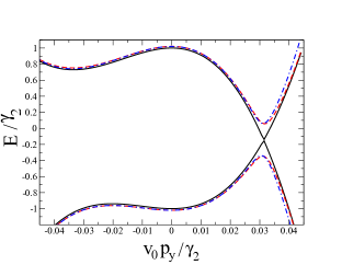
Figure 2: Low-energy bands of ABC trilayer graphene at the $K$ point as a function of $p_{y}$ for $p_{x}=0$: using the full $\mathbf{k}\cdot\mathbf{p}$ Hamiltonian with zero spin-orbit coupling (solid, black), with finite spin-orbit coupling (red, dashed), and using the effective Hamiltonian $\hat{H}^{\rm eff}_{ABC}$ (dashed-dotted, blue). The parameters $v_{i}$ were taken from Ref. macdonald-1, and we have chosen $\lambda_{1/2}=\lambda_{1}=0.2\,\gamma_{2}$.

VII Substrate induced SOC

The calculations of Sect. III - V suggest that the intrinsic SOC in ABC trilayer is relatively small, the order of magnitude of the SOC parameters is $10\mu{\rm eV}$, the same as in monolayerboettger ; jfabian-so-numeric ; jfabian-mono-TB ; abdelouahed or bilayerjfabian-bilayer graphene. One can, in principle, enhance the SOC in a number of ways, e.g. by impuritiescastro-neto , by applying strong external electric fieldjfabian-bilayer , making the graphene sheet curvedklimovaja-curvedbi , using adatoms with large atomic numbergraphene-adatom ; graphene-adatom-2 ; graphene-adatom-3 or bringing the trilayer into proximity with a suitable substrateproximity-spin-orbit ; varykhalov-nature . Since proximity to a substrate or adatoms is likely to lead to a larger SOC effect than what one can induce by an external electric field, here we consider an effective model whereby strong SOC is induced in one of the outer layers of trilayer graphene whereas SOC is not altered in the other two layers. For concreteness, we assume that it is the first graphene layer where strong SOC is induced and for simplicity we will refer both to the scenario involving a substrate and that involving adatoms as ”substrate induced SOC“. From the symmetry point of view, the model we consider here is not exact: a group theoretical analysisdresselhaus-book ; dresselhaus-paper ; jfabian-bilayer of the matrix elements of the SOC Hamiltonian shows that by breaking the inversion symmetry there can be in principle $21$ different SOC parameters. However, we assume that all intra and interlayer SOC parameters will remain small with respect to the SOC parameters in the layer that is in the immediate proximity of the substrate. The relevant part of the SOC Hamiltonian that we consider as a minimal model is shown in Table 5. We assume that at the $K$ point of the BZ only four SOC parameters have significant values and neglect all other intra or inter-layer coupling spin-orbit parameters.

SOC	$\Psi^{A1}_{\rm eff}$	$\Psi^{B3}_{\rm eff}$	$\Psi^{B1}_{\rm eff}$
$\Psi^{A1}_{\rm eff}$	$\tilde{\lambda}_{1/2}S_{z}$	$0$	$\lambda_{BR}S_{+}^{\tau}$
$\Psi^{B3}_{\rm eff}$	$0$	$-\lambda_{1/2}S_{z}$	$0$
$\Psi^{B1}_{\rm eff}$	${\lambda}_{BR}S_{-}^{\tau}$	$0$	$-\tilde{\lambda}_{3/3}^{z}S_{z}$

Table 5: The non-zero part of the model SOC Hamiltonian $\tau\,\tilde{H}_{so}^{ext}$ .

The SOC parameters that we keep are $\tilde{\lambda}_{1/2}$ and $\tilde{\lambda}_{3/3}^{z}$ which may describe enhanced diagonal SOC on $A1$ and $B1$ type atoms, respectively, whereas $\lambda_{BR}$ is the Bychkov-Rashbarashba type SOC acting only in the first graphene layer. Since we are going to derive an effective low-energy Hamiltonian, we also keep non-zero the intrinsic SOC parameter $\lambda_{1/2}$ on atom $B3$, which, however, might be much smaller than $\tilde{\lambda}_{1/2}$ and $\tilde{\lambda}_{3/3}^{z}$.

Similarly to Sect. VI, for the full Hamiltonian of the system in the vicinity of the $K$ point we take $\tilde{H}_{ABC}=\tilde{H}_{\mathbf{k}\cdotp\mathbf{p}}^{ABC}+\tilde{H}_{so}^{ext}$. In the Hamiltonian $\tilde{H}_{\mathbf{k}\cdotp\mathbf{p}}^{ABC}$, as an additional substrate effect, we also include a possible shift $\Delta$ of the on-site energies of atoms $A1$ and $B1$ with respect to atoms in the other two layers. (Otherwise $\tilde{H}_{\mathbf{k}\cdotp\mathbf{p}}^{ABC}$ is the same as in Section VI.) To study the low energy physics we again use the Schrieffer-Wolff transformation to eliminate the high-energy bands. The hopping $\gamma_{1}$ is treated as a large energy scale with respect to $v_{0}\pi$, $|\gamma_{3}|$, $\gamma_{4}$, $\gamma_{2}$, $\Delta$ and we keep only the leading order for the terms involving $\Delta$, $\gamma_{2}$, $v_{3}$ and $v_{4}$. The electronic part $\hat{\tilde{H}}^{\rm eff}_{el}$ of the effective Hamiltonian $\hat{\tilde{H}}^{\rm eff}_{ABC}$ contains one new term in addition to the terms in Eq. (13):

$$\hat{H}_{\Delta}=\Delta\left[\left(\begin{array}[]{cc}1&0\\ 0&0\end{array}\right)-\frac{v_{0}^{2}}{2\gamma_{1}^{2}}\left(\begin{array}[]{cc}2\pi^{\dagger}\pi+\pi\pi^{\dagger}&0\\ 0&-\pi\pi^{\dagger}\end{array}\right)\right].$$ (16)

Up to linear order in the momentum and the SOC parameters the effective spin-orbit Hamiltonian has the following terms:

$$\hat{\tilde{H}}_{so}^{ABC} = \left[\hat{\tilde{H}}_{so}^{ABC,(0)}+\hat{\tilde{H}}_{so}^{ABC,(1)}+\hat{\tilde{H}}_{so}^{ABC,(2)}\right],$$

$$\hat{\tilde{H}}_{so}^{ABC,(0)} = \tau\,S_{z}\left(\begin{array}[]{cc}\tilde{\lambda}_{1/2}&0\\ 0&-\lambda_{1/2}\end{array}\right),$$ (17c)

$$\hat{\tilde{H}}_{so}^{ABC,(1)} = -\tau\,\lambda_{BR}\frac{v_{3}}{\gamma_{1}}\left(\begin{array}[]{cc}0&S_{+}^{\tau}\pi\\ S_{-}^{\tau}\pi^{\dagger}&0\\ \end{array}\right),$$ (17f)

$$\hat{\tilde{H}}_{so}^{ABC,(2)} = -\tau\,\lambda_{BR}\frac{v_{4}}{\gamma_{1}}(S_{-}^{\tau}\pi^{\dagger}+S_{+}^{\tau}\pi)\left(\begin{array}[]{cc}1&0\\ 0&0\end{array}\right).$$ (17i)

It is interesting to compare this result to what one obtains for bilayer graphene using the same modelsimple-so-bilayer :

$$\hat{\tilde{H}}_{so}^{AB} = \tau\cdotp\left[\hat{\tilde{H}}_{so}^{AB,(0)}+\hat{\tilde{H}}_{so}^{AB,(1)}+\hat{\tilde{H}}_{so}^{AB,(2)}\right],$$

$$\hat{\tilde{H}}_{so}^{AB,(0)} = S_{z}\left(\begin{array}[]{cc}\tilde{\lambda}_{3/3}^{z}&0\\ 0&-\lambda_{3/3}^{z}\end{array}\right),$$ (18c)

$$\hat{\tilde{H}}_{so}^{AB,(1)} = -\lambda_{BR}\frac{v_{0}}{\gamma_{1}}\left(\begin{array}[]{cc}0&S_{+}^{\tau}\pi^{\dagger}\\ S_{-}^{\tau}\pi&0\\ \end{array}\right),$$ (18f)

$$\hat{\tilde{H}}_{so}^{AB,(2)} = -\lambda_{BR}\frac{v_{4}}{\gamma_{1}}(S_{-}^{\tau}\pi^{\dagger}+S_{+}^{\tau}\pi)\left(\begin{array}[]{cc}1&0\\ 0&0\end{array}\right).$$ (18i)

In the appropriate limit Hamiltonian (18) agrees with the result of Ref. jfabian-bilayer, . Similar models have also been considered in two recent works: In Ref. mireles, strong Rashba SOC was assumed in both layers of bilayer graphene and a linear-in-momentum low-energy SOC Hamiltonian was derived, whereas in Ref. prada, the authors kept only the first term, $\hat{\tilde{H}}_{so}^{AB,(0)}$ and set $\lambda_{3/3}^{z}=0$.

One can see that in contrast to monolayer graphene, in bilayer and ABC trilayer graphene the Rashba SOC affects the spin-dynamics in the low-energy bands through terms which are momentum dependentsecond-order-soi . This means that at the $K$ ($K^{\prime}$) point the effect of Rashba-type SOC is suppressed with respect to monolayer graphene. Furthermore, noting that $v_{0}\gg v_{3}$, a comparison of the prefactors of $\hat{\tilde{H}}_{so}^{ABC,(1)}$ and $\hat{\tilde{H}}_{so}^{AB,(1)}$ may suggest that the influence of linear-in-momentum terms on spin-dynamics might be more important in bilayer than in trilayer. This is, strictly speaking, only true in the model that we used, i.e when other off-diagonal SOC parameters can be neglected with respect to $\lambda_{BR}$. In general, there would be a linear-in-momentum SOC Hamiltonian with a pre-factor proportional to $v_{0}/\gamma_{1}$ for the trilayer case as well. The model introduced above could be relevant e.g. in an experiment similar to Ref. varykhalov-nature, if bilayer or trilayer is used instead of monolayer graphene. Varykhalov et alvarykhalov-nature reported a large Rashba SOC in monolayer graphene with $\lambda_{BR}$ between $10-100\,{\rm meV}$, whereas, as we have seen, the intrinsic SOC parameters are typically of a few $10\mu{\rm eV}$.

A detailed study of the properties of Hamiltonians (17) and (18) is left for a future study. We expect a rich physics emerging from the interplay of diagonal and off-diagonal spin-orbit terms and the interlayer asymmetry $\Delta$.

VIII Conclusions

In conclusion, we studied the intrinsic and substrate induced spin-orbit interaction in bilayer and ABC trilayer graphene. Assuming that in flat graphene systems the most important contribution to the SOC comes from the admixture of $p_{z}$ and $d$ orbitals and using a combination of group-theoretical and tight-binding approaches we derived the intrinsic SOC Hamiltonian of ABC trilayer graphene. In contrast to the similar calculations for monolayer graphenejfabian-mono-TB , we found that in bilayer and ABC trilayer in addition to $d_{xz}$ and $d_{yz}$ orbitals also $d_{z^{2}}$ orbitals have to be taken into account. For both bilayer and trilayer graphene we obtained explicit expressions for the SOC parameters in terms of SK hopping parameters. By comparing these expressions with the DFT calculations of Ref. jfabian-bilayer, , we were able to estimate the values of the intrinsic SOC constants for ABC trilayer graphene. Since the intrinsic SOC is quite small, we considered a situation when adatoms or a substrate can induce a strong SOC (intrinsic diagonal or Rashba type off-diagonal) in only one of the layers of bilayer and ABC trilayer graphene. To describe the low-energy physics we derived effective Hamiltonians for both systems. We found that the effect of Rashba type SOC is suppressed close to the $K$ ($K^{\prime}$) point with respect to monolayer graphene.

The approach that we used here to derive the SOC Hamiltonians can be employed in the case of other related problems as well. For instance ABA stacked trilayer graphene or graphite can be treated on the same footing when one takes into account, that they have different symmetries from bilayer and ABC trilayer graphene. Considering the substrate induced SOC, which can be strong enough to make the SOC related phenomena experimentally observable, one interesting question is whether the different symmetries and band structure of ABC and ABA trilayer would manifest themselves in e.g. significantly different spin-transport properties.

IX Acknowledgments

We acknowledge funding from the DFG within SFB 767 and from the ESF/DFG within the EuroGRAPHENE project CONGRAN.

Appendix A Small group of the K point and basis functions

The relevant symmetry group for the calculations at the $K$ point for both trilayer and bilayer graphene is the group $32$ ($D_{3}$). The generators of this group are two three fold rotations ($C_{3}$) around an axis perpendicular to the plane of the graphene layers and three two-fold rotations ($C_{2}$). There are three irreducible representations, two one-dimensional denoted by $\Gamma_{A_{1}}$, $\Gamma_{A_{2}}$ and a two-dimensional one, $\Gamma_{E}$ (see Table 6).

$32\,(D_{3})$	$E$	$2C_{3}$	$3C_{2}$
$\Gamma_{A_{1}}$	$1$	$1$	$1$
$\Gamma_{A_{2}}$	$1$	$1$	$-1$
$\Gamma_{E}$	$2$	$-1$	$0$

Table 6: Character table of the group $32$ ($D_{3}$).

The basis functions built from the linear combinations of $p_{z}$ and $d$ orbitals which transform as these irreducible representations are shown in Table 7 for ABC trilayer and in Table 8 for bilayer.

$\Gamma_{A_{1}}$	$|\overline{\Psi_{1,0,0}^{1,3}}\rangle$, $|\Psi_{2,1,-1}^{3,1}\rangle$, $|\Psi_{2,0,0}^{1,3}\rangle$, $|\Psi_{2,-2,2}^{3,1}\rangle$, $|\Psi_{2,-1,1}^{2,2}\rangle$, $|\Psi_{2,2,-2}^{2,2}\rangle$
$\Gamma_{A_{2}}$	$|{\Psi_{1,0,0}^{1,3}}\rangle$, $|\overline{\Psi_{2,1,-1}^{3,1}}\rangle$, $|\overline{\Psi_{2,0,0}^{1,3}}\rangle$, $|\overline{\Psi_{2,-2,2}^{3,1}}\rangle$, $|\overline{\Psi_{2,-1,1}^{2,2}}\rangle$, $|\overline{\Psi_{2,2,-2}^{2,2}}\rangle$
$\Gamma_{E}$	$\{|{\Psi_{1,0,0}^{2,1}}\rangle,|{\Psi_{1,0,0}^{3,2}}\rangle\}$, $\{|\overline{\Psi_{1,0,0}^{2,1}}\rangle,|\overline{\Psi_{1,0,0}^{3,2}}\rangle\}$
	$\{|{\Psi_{2,0}^{A2}}\rangle,|{\Psi_{2,0}^{B2}}\rangle\}$, $\{|{\Psi_{2,1}^{A2}}\rangle,|{\Psi_{2,-1}^{B2}}\rangle\}$, $\{|{\Psi_{2,-2}^{A2}}\rangle,|{\Psi_{2,2}^{B2}}\rangle\}$
	$\{|{\Psi_{2,0}^{A3}}\rangle,|{\Psi_{2,0}^{B1}}\rangle\}$, $\{|{\Psi_{2,-1}^{A3}}\rangle,|{\Psi_{2,1}^{B1}}\rangle\}$, $\{|{\Psi_{2,2}^{A3}}\rangle,|{\Psi_{2,-2}^{B1}}\rangle\}$
	$\{|{\Psi_{2,1}^{A1}}\rangle,|{\Psi_{2,-1}^{B3}}\rangle\}$, $\{|{\Psi_{2,-1}^{A1}}\rangle,|{\Psi_{2,1}^{B3}}\rangle\}$, $\{|{\Psi_{2,2}^{A1}}\rangle,|{\Psi_{2,-2}^{B3}}\rangle\}$
	$\{|{\Psi_{2,-2}^{A1}}\rangle,|{\Psi_{2,2}^{B3}}\rangle\}$

Table 7: Basis functions for the irreducible representations of the small group of the $K$ point for ABC trilayer graphene. The basis functions for the $K^{\prime}$ point can be obtained by complex-conjugation.

$\Gamma_{A_{1}}$	$|\overline{\Psi_{1,0,0}^{2,1}}\rangle$, $|\Psi_{2,1,-1}^{1,2}\rangle$, $|\Psi_{2,0,0}^{2,1}\rangle$, $|\Psi_{2,-2,2}^{2,1}\rangle$
$\Gamma_{A_{2}}$	$|{\Psi_{1,0,0}^{2,1}}\rangle$, $|\overline{\Psi_{2,1,-1}^{1,2}}\rangle$, $|\overline{\Psi_{2,0,0}^{2,1}}\rangle$, $|\overline{\Psi_{2,-2,2}^{2,1}}\rangle$
$\Gamma_{E}$	$\{|{\Psi_{1,0}^{A1}}\rangle,|{\Psi_{1,0}^{B2}}\rangle\}$, $\{|{\Psi_{2,0}^{A1}}\rangle,|{\Psi_{2,0}^{B2}}\rangle\}$, $\{|{\Psi_{2,-1}^{A1}}\rangle,|{\Psi_{2,1}^{B2}}\rangle\}$
	$\{|{\Psi_{2,2}^{A1}}\rangle,|{\Psi_{2,-2}^{B2}}\rangle\}$, $\{|{\Psi_{2,-2}^{A1}}\rangle,|{\Psi_{2,2}^{B1}}\rangle\}$, $\{|{\Psi_{2,-1}^{A2}}\rangle,|{\Psi_{2,1}^{B1}}\rangle\}$
	$\{|{\Psi_{2,1}^{A2}}\rangle,|{\Psi_{2,-1}^{B1}}\rangle\}$, $\{|{\Psi_{2,2}^{A2}}\rangle,|{\Psi_{2,-2}^{B1}}\rangle\}$

Table 8: The same as in Table 7 but for bilayer graphene.

In the case of bilayer, making then the same steps as for trilayer graphene, one finds the symmetry basis and intrinsic SOC parameters given in Table 9.

$|\Psi_{\Gamma_{A_{1}}}\rangle=|\overline{\Psi_{1,0,0}^{2,1}}\rangle+\frac{3}{\sqrt{2}}\frac{V_{pd\pi}}{\delta\varepsilon_{pd}-\gamma_{1}}|\Psi_{2,1,-1}^{1,2}\rangle-\frac{{V}_{pd\sigma}}{\delta\varepsilon_{pd}-\tilde{\gamma}_{1}}|\Psi_{2,0,0}^{2,1}\rangle$	$\lambda_{1/2}=-\frac{9}{2}\,\xi_{d}\,\frac{(V_{pd\pi})^{2}}{(\delta\varepsilon_{pd}^{2}-\gamma_{1}^{2})}$
$|\Psi_{\Gamma_{A_{2}}}\rangle=|\Psi_{1,0,0}^{2,1}\rangle-\frac{3}{\sqrt{2}}\frac{V_{pd\pi}}{\delta\varepsilon_{pd}+\gamma_{1}}|\overline{\Psi_{2,1,-1}^{1,2}}\rangle+\frac{{V}_{pd\sigma}}{\delta\varepsilon_{pd}+\tilde{\gamma}_{1}}|\overline{\Psi_{2,0,0}^{2,1}}\rangle$	$\lambda_{1/3}=-3\sqrt{\frac{3}{2}}\,\xi_{d}\,\frac{V_{pd\pi}{V}_{pd\sigma}}{\delta\varepsilon_{pd}(\delta\varepsilon_{pd}-\tilde{\gamma}_{1})}$
$|\Psi_{\Gamma_{E_{1,1}}}\rangle=|\Psi_{1,0}^{A1}\rangle+\frac{3}{\sqrt{2}}\frac{V_{pd\pi}}{\delta\varepsilon_{pd}}|\Psi_{2,-1}^{B1}\rangle$	$\lambda_{2/3}=-3\sqrt{\frac{3}{2}}\,\xi_{d}\,\frac{V_{pd\pi}{V}_{pd\sigma}}{\delta\varepsilon_{pd}(\delta\varepsilon_{pd}+\tilde{\gamma}_{1})}$
$|\Psi_{\Gamma_{E_{1,2}}}\rangle=|\Psi_{1,0}^{B2}\rangle-\frac{3}{\sqrt{2}}\frac{V_{pd\pi}}{\delta\varepsilon_{pd}}|\Psi_{2,1}^{A2}\rangle$	$\lambda_{3/3}^{z}=-\frac{9}{2}\,\xi_{d}\,\frac{(V_{pd\pi})^{2}}{\delta\varepsilon_{pd}^{2}}$

Table 9: Symmetry basis functions (left column) and intrinsic spin-orbit matrix elements (right column) in terms of Slater-Koster parameters for bilayer graphene. We used the notation $V_{pd\sigma}=V_{pd\sigma}^{A2,B1}$, $\delta\varepsilon_{pd}=\varepsilon_{p}-\varepsilon_{d}$ and $\tilde{\gamma}_{1}=\gamma_{1}+V_{dd\sigma}$.

Referring to Fig. 1(a), the atomic sites participating in the formation of the split-off bands are denoted by $B1$ and $A2$, whereas they are labeled as $A1$ and $B2$ in Ref. jfabian-bilayer, , and similarly for the sites contributing to the low energy bands. Therefore, to arrive at the SOC Hamiltonian shown in Table 4, (i) one has to rotate the symmetry basis into the on-site basis, (ii) re-label the sites as $Aj\leftrightarrows Bj$, (iii) and make the identification $\lambda_{\rm I1}=-\lambda_{3/3}^{z}$, $\lambda_{\rm I2}=-\lambda_{1/2}$, $\lambda_{0}=\frac{1}{\sqrt{2}}(\lambda_{2/3}-\lambda_{1/3})$, $\lambda_{4}^{bi}=-\frac{1}{\sqrt{2}}(\lambda_{2/3}+\lambda_{1/3})$. The matrix elements are real numbers in our calculations because we use different lattice vectors than in Ref. jfabian-bilayer, .

Appendix B

Here we collect some useful formulae: We give explicitly the transformation between the symmetry basis and the effective on-site $p_{z}$ orbital basis for the trilayer case and present the low-energy electronic Hamiltonian for bilayer graphene.

B.1 Transformation between the symmetry basis and the on-site effective $p_{z}$ basis

The transformation reads:

$$\left(\begin{array}[]{c}|\Psi^{A1}_{\rm eff}\rangle\\ |\Psi^{B3}_{\rm eff}\rangle\\ |\Psi^{B1}_{\rm eff}\rangle\\ |\Psi^{A2}_{\rm eff}\rangle\\ |\Psi^{B2}_{\rm eff}\rangle\\ |\Psi^{A3}_{\rm eff}\rangle\end{array}\right)=\frac{1}{\sqrt{2}}\left(\begin{array}[]{cccccc}1&1&0&0&0&0\\ -1&1&0&0&0&0\\ 0&0&1&0&-1&0\\ 0&0&1&0&1&0\\ 0&0&0&1&0&-1\\ 0&0&0&1&0&1\\ \end{array}\right)\left(\begin{array}[]{c}|\Psi_{\Gamma_{A_{1}}}\rangle\\ |\Psi_{\Gamma_{A_{2}}}\rangle\\ |\Psi_{\Gamma_{E_{1,1}}}\rangle\\ |\Psi_{\Gamma_{E_{1,2}}}\rangle\\ |\Psi_{\Gamma_{E_{2,1}}}\rangle\\ |\Psi_{\Gamma_{E_{2,2}}}\rangle\end{array}\right).$$ (19)

B.2 Bilayer graphene low-energy electronic Hamiltonian

For completeness and for comparison with the trilayer case given in Eq. (13), we show here the low-energy electronic Hamiltonian of bilayer graphene in the on-site basis $A1$, $B2$. This Hamiltonian has been discussed in many publications before, see e.g. the recent review of Ref. mccann-koshino-bilayer, . As in Sect. VII, we assume that atoms $A1$ and $B1$ in the layer adjacent to the substrate have a different on-site energy $\Delta$ than atoms $A2$, $B2$ in the second layer. The most important terms are found to be:

$${\hat{H}}^{\rm\,eff}_{el} = {\hat{H}}_{chir}+{\hat{H}}_{3w}+{\hat{H}}_{v_{4}}+\hat{H}_{\Delta},$$

$${\hat{H}}_{chir} = -\frac{v_{0}^{2}}{\gamma_{1}}\left(\begin{array}[]{cc}0&\left({\pi}^{{\dagger}}\right)^{2}\\ {\pi^{2}}&0\end{array}\right),\,\,\,\hat{H}_{3w}=v_{3}\left(\begin{array}[]{cc}0&\pi\\ \pi^{\dagger}&0\end{array}\right),$$ (24)

$${\hat{H}}_{v_{4}} = -\frac{2v_{0}v_{4}}{\gamma_{1}}\left(\begin{array}[]{cc}\pi^{\dagger}\pi&0\\ 0&\pi\pi^{\dagger}\end{array}\right),$$ (27)

$$\hat{H}_{\Delta} = \Delta\left[1-\frac{v_{0}^{2}}{2\gamma_{1}^{2}}\pi^{\dagger}\pi\right]\left(\begin{array}[]{cc}\texttimes 1&0\\ 0&0\end{array}\right).$$ (30)

References

- (1) A. H. Castro Neto, F. Guinea, N. M. R. Peres, K. S. Novoselov, and A. K. Geim, Rev. Mod. Phys 81, 109 (2009).
- (2) F. Guinea, A. H. Castro Neto, and N. M. R. Peres, Phys. Rev. B 73, 245426 (2006).
- (3) S. Latil and L. Henrard, Phys. Rev. Lett. 97, 036803 (2006).
- (4) C. L. Lu, C. P. Chang, Y. C. Huang, R. B. Chen, and M. L. Lin Phys. Rev. B 73, 144427 (2006).
- (5) M. Aoki and H. Amawashi, Solid State Commun. 142, 123 (2007).
- (6) B. Partoens and F. M. Peeters Phys. Rev. B 75, 193402 (2007).
- (7) A. Grüneis, C. Attaccalite, L. Wirtz, H. Shiozawa, R. Saito, T. Pichtler, and A. Rubio, Phys. Rev. B 78, 205425 (2008).
- (8) M. Koshino and E. McCann, Phys. Rev. B 80, 165409 (2009).
- (9) M. Koshino and E. McCann Phys. Rev. B 79, 125443 (2009).
- (10) M. Koshino, Phys. Rev. B 81 125304 (2010).
- (11) F. Zhang, B. Sahu, H. Min, and A. H. MacDonald, Phys. Rev. B 82, 035409 (2010).
- (12) K. F. Mak, J. Shan, and T. F. Heinz, Phys. Rev. Lett. 104, 176404 (2010).
- (13) Ch. H. Lui, Zh. Li, Zh. Chen, P. V. Klimov, L. E. Brus, and T. F. Heinz, Nano Lett 11, 164 (2011).
- (14) Ch. H. Lui, Zh. Li, K. F. Mak, E. Cappelluti and T. F. Heinz, Nature Physics 7, 944 (2011).
- (15) W. Bao, L. Jing, J. Velasco Jr, Y. Lee, G. Liu, D. Tran, B. Standley, M. Ayko, S. B. Cronin, D. Smirnov, M. Koshino, E. McCann, M. Bockrath, and C. N. Lau, Nature Physics 7, 948 (2011).
- (16) L. Zhang, Y. Zhang, J. Camacho, M. Khodas, and I. Zaliznyak, Nature Physics 7, 953 (2011).
- (17) Th. Taychatanapat, K. Watanabe, T. Taniguchi, and P. Jarillo-Herrero, Nature Physics 7, 621 (2011).
- (18) T. Khodkov, F. Withers, D. Ch. Hudson, M. F. Craciun, and S. Russo, Appl. Phys. Lett. 100, 013114 (2012).
- (19) A. A. Avetisyan, B. Partoens, and F. M. Peeters, Phys. Rev. B 81, 115432 (2010).
- (20) R. Xiao, F. Tasnádi, K. Koepernik, J. W. F. Venderbos, M. Richter, and M. Taut Phys. Rev. B 84, 165404 (2011).
- (21) F. Zhang, J. Jung, G. A. Fiete, Q. Niu, and A. H. MacDonald, Phys. Rev. Lett. 106, 156801 (2011).
- (22) F. Zhang, D. Tilahun, A. H. MacDonald Phys. Rev. B 85, 165139 (2012).
- (23) Y. Barlas, R. Cote, and M. Rondeau, Phys. Rev. Lett. 109, 126804 (2012).
- (24) V. Cvetković and O. Vafek, arXiv:1210.4923 (unpublished).
- (25) J. Güttinger, C. Stampfer, F. Molitor, D. Graf, T. Ihn, and K. Ensslin, New J. Phys. 10, 125029 (2008).
- (26) M. F. Craciun, S. Russo, M. Yamamoto, J. B. Oostinga, A. F. Morpurgo and S. Tarucha, Nat. Nanotechnology 4, 383 (2009)
- (27) A. Kumar, W. Escoffier, J. M. Poumirol, C. Faugeras, D. P. Arovas, M. M. Fogler, F. Guinea, S. Roche, M. Goiran, and B. Raquet, Phys. Rev. Lett. 107, 126806 (2011).
- (28) E. V. Castro, M. P. López-Sancho, and M. A. H. Vozmediano, Solid State Commun. 152, 1483 (2012).
- (29) E. McCann and M. Koshino, Phys. Rev. B 81, 241409(R) (2010).
- (30) F. Guinea, New Journal of Physics, 12, 083063 (2010).
- (31) C. Ertler, S. Konschuh, M. Gmitra, and J. Fabian Phys. Rev. B 80, 041405(R) (2009).
- (32) E. McCann and V. I. Fal’ko, Phys. Rev. Lett. 108, 166606 (2012).
- (33) H. Ochoa, A. H. Castro Neto, and F. Guinea Phys. Rev. Lett. 108, 206808 (2012).
- (34) M. Diez and G. Burkard, Phys. Rev. B 85, 195412 (2012).
- (35) C. L. Kane and E. J. Mele, Phys. Rev. Lett. 95, 226801 (2005).
- (36) B. Dlubak, M.-B. Martin, C. Deranlot, B. Servet, S. Xavier, R. Mattana, M. Sprinkle, C. Berger, W. A. De Heer, F. Petroff, A. Anane, P. Seneor, and A. Fert, Nature Physics 8, 557 (2012).
- (37) M. Gmitra, S. Konschuh, Ch. Ertler, C. Ambrosch-Draxl, and J. Fabian, Phys. Rev. B 80, 235431 (2009).
- (38) S. Abdelouahed, A. Ernst, J. Henk, I. V. Maznichenko, and I. Mertig, Phys. Rev. B 82, 125424 (2010).
- (39) S. Konschuh, M. Gmitra, and J. Fabian, Phys. Rev. B 82, 245412 (2010).
- (40) S. Konschuh, M. Gmitra, D. Kochan, and J. Fabian, Phys. Rev. B 85, 115423 (2012).
- (41) J. C. Slater and G. F. Koster, Phys. Rev. 94, 1498 (1954).
- (42) G. Dresselhaus and M. S. Dresselhaus, Phys. Rev. 140, A401 (1965).
- (43) M. S. Dresselhaus, G. Dresselhaus and A. Jorio, Group Theory, Springer-Verlag Berlin Heidelberg (2008).
- (44) J. C. Boettger, and S. B. Trickey, Phys. Rev. B 75, 121402 (2007).
- (45) S. Konschuh, Spin-Orbit Coupling Effects From Graphene To Graphite, PhD thesis, University Regensburg (2011).
- (46) R. Winkler, Spin-Orbit Coupling Effects in Two-Dimensional Electron and Hole Systems, Springer-Verlag Berlin Heidelberg (2003).
- (47) S. Bravyi, D. DiVincenzo, and D. Loss, Ann. Phys. 326, 2793 (2011).
- (48) Zero matrix elements can arise e.g. because we neglect remote direct hoppings between the first and the third layer except for the hopping -.
- (49) The approximation can be justified by the numerical calculations of Ref. jfabian-mono-TB, . There it was shown that in the case of monolayer graphene . Since is a small energy scale compared to , we find that . Furthermore, since and correspond to hopping between and atoms which are at larger distance than the and atoms within the same graphene layer, one can expect that and , hence both matrix elements of in Eq. (7) are much smaller than unity.
- (50) Ref. guinea-so, considers an effective one-layer model and obtains a SOC Hamiltonian which is wavenumber independent and can be characterized by two SOC constants. One of the SO parameters, denoted by in Ref. guinea-so, , corresponds to our . This can be seen by folding down the full Hamiltonian to obtain a low-energy effective model [see Eq. (15) in Sect. VI]. Further wavenumber-independent SOC terms can also be obtained from the folding down procedure, but they are higher order in the SOC parameters. Therefore we think that they are negligible with respect to the effective SOC Hamiltonian shown in Eq. (15). Ref. [konschuh-phd, ] explains the numerically calculated band structure with a single, diagonal SOC parameter.
- (51) A. H. Castro Neto and F. Guinea, Phys. Rev. Lett. 103, 026804 (2009).
- (52) J. Klimovaja, G. J. Ferreira, and D. Loss, Phys. Rev. B 86, 235416 (2012).
- (53) C. Weeks, Jun Hu, J. Alicea, M. Franz, and Ruqian Wu, Phys. Rev. X 1, 021001 (2011).
- (54) O. Shevtsov, P. Carmier, C. Groth, X. Waintal, and D. Carpentier, Phys. Rev. B 85, 245441 (2012).
- (55) H. Jiang, Zh. Qiao, H. Liu, J. Shi, and Q. Niu, Phys. Rev. Lett. 109, 116803 (2012).
- (56) K.-H. Jin, S.-H. Jhi, arXiv:1206.3608 (unpublished).
- (57) D. Marchenko, A. Varykhalov, M. R. Scholz, G. Bihlmayer, E. I. Rashba, A. Rybkin, A. M. Shikin, and O. Rader arXiv:1208.4265 (unpublished).
- (58) E. I. Rashba, Phys. Rev. B 79, 161409 (2009).
- (59) In general, if the inversion symmetry is broken there are ten SOC parameters in bilayer graphene. As in Ref. jfabian-bilayer, , we keep only the most important ones.
- (60) E. Prada, P. San-Jose, L. Brey, and H. A. Fertig, Solid State Communications 151, 1075 (2011).
- (61) F. Mireles and J. Schliemann, New J. Phys. 14, 093026 (2012).
- (62) More precisely, as we have already mentioned in connection with the intrinsic SOCtwo-soc-param , when one folds down the full Hamiltonian one can obtain additional momentum-independent terms for the low-energy Hamiltonian but they are proportional to products and higher powers of the SOC parameters. We neglect these terms.
- (63) E. McCann and M. Koshino, arXiv:1205.6953 (unpublished).