Self-bound quark matter in the NJL model revisited:
from schematic droplets to domain-wall solitons

Abstract

The existence and the properties of self-bound quark matter in the NJL model at zero temperature are investigated in mean-field approximation, focusing on inhomogeneous structures with one-dimensional spatial modulations. It is found that the most stable homogeneous solutions which have previously been interpreted as schematic quark droplets are unstable against formation of a one-dimensional lattice of domain-wall solitons. The solitons repel each other, so that the minimal energy per quark is realized in the single-soliton limit. The properties of the solitons and their interactions are discussed in detail, and the effect of vector interactions is estimated. The results may be relevant for the dynamics of expanding quark matter.

I Introduction

The Nambu–Jona-Lasinio (NJL) model NJL is a popular tool for studying low-energy properties of strongly interacting matter, like spectra and scattering of light hadrons, or the phase diagram at nonvanishing temperatures or densities (for reviews, see Refs. Vogl:1991qt ; Klevansky:1992qe ; Hatsuda:1994pi ; Buballa:2005 ). While being relatively simple, the NJL model shares the global symmetries of QCD, in particular chiral symmetry, which is considered to be the most important feature of the model. On the other hand, it is well known that the NJL model lacks confinement. In this sense it can be viewed as complementary to the MIT bag model MIT , which is confining by construction, but violates chiral symmetry at the surface.

Some time ago, it was realized, however, that for sufficiently attractive interactions, the NJL model at zero temperature has solutions of self-bound chirally restored quark matter, which can be interpreted as bag-model-like quark droplets Buballa:2005 ; Buballa:1996tm ; Alford:1997zt ; Buballa:1998ky . In fact, the link between both models is the existence of a “bag pressure”, which in the bag model is introduced by hand in order to stabilize the solutions, whereas in the NJL model it is a dynamical consequence of spontaneous chiral symmetry breaking in vacuum.

The self-bound quark matter solutions mentioned above have been obtained in the thermodynamic limit and correspond to infinite homogeneous matter. Their interpretation as quark-matter droplets is based on the behavior of the energy per particle, $E/N$, which shows a minimum at some nonvanishing saturation density. This means, a finite piece of quark matter with this density would be stable against collapse or expansion, just like a liquid drop.

An equivalent statement is that the matter has vanishing pressure, which means, it is in mechanical equilibrium with the vacuum. Thus, in order to have a solution of this type, there must be a phase coexistence of the vacuum with a dense-matter phase. In other words, at some critical chemical potential, there must be a first-order phase transition from the vacuum to dense matter. This is realized in the NJL model, if the interaction is sufficiently attractive. On the other hand, if the attraction is relatively weak (a condition which can be achieved, e.g., by adding a repulsive vector interaction), it is also possible to have a second-order phase transition or a crossover. In this case there is no stable matter solution and $E/N$ takes its minimal value at zero density. Without applying external forces, a finite piece of quark matter would then keep expanding, i.e., behave like a gas.

It is tempting at this point to extrapolate the self-bound solutions down to droplets consisting of only three quarks, and to interpret them as baryons. However, although some of the resulting “baryon” properties are quite reasonable Buballa:1996tm , it is obvious that this extrapolation is not reliable. In fact, using solutions for infinite homogeneous quark matter to describe finite droplets, one has to assume that surface effects can be neglected. This assumption might be justified for large droplets but most likely not for small ones. Besides, if the surface tension is positive, as derived, e.g., in Refs. Molodtsov:2011ii ; Lugones:2011xv ; Pinto:2012aq , smaller droplets are disfavored. The preferred state in the model would therefore be a configuration where all quarks are joined in one big spherical nugget, rather than hadronized into individual baryons.

It turns out, however, that this is not quite the case. More recent studies of the NJL phase diagram have revealed that the first-order chiral phase transition between homogeneous phases gets replaced by an inhomogeneous region if one allows the chiral condensate to be nonuniform in space Sadzikowski:2000ap ; Nakano:2004cd ; Nickel:2009wj . In this region, a special class of solutions, which vary in one spatial dimension, has been found to be favored over all other shapes considered so far. These solutions correspond to a lattice of domain-wall solitons described in terms of Jacobi elliptic functions and smoothly interpolate between the homogeneous chirally broken and restored phases Nickel:2009wj . In particular at the low-density side, they take the form of a single soliton, which is thermodynamically degenerate with the homogeneous chirally broken phase. As a consequence, the phase transition to the latter is of second order.

This changes our picture of self-bound quark matter in the NJL model considerably. Since there is no longer a first-order phase transition connecting the vacuum with a finite-density phase, but a second-order phase transition to the inhomogeneous phase, the minimal $E/N$ should now be reached at zero average density. However, unlike the homogeneous case where the low-density regime corresponds to a dilute gas of constituent quarks, we now expect a “liquid crystal” of well separated solitons. These objects have a nonvanishing quark density and a finite size in one spatial dimension, while being infinite in the remaining two dimensions. This could be seen as a step towards “real” quark droplets, which are finite in three dimensions.

In the present article we perform an explicit model study to investigate the scenario outlined above quantitatively. After briefly introducing the formal background, we calculate $E/N$ as a function of the average density and compare the results for inhomogeneous solutions with those for homogeneous matter. Based on these results, we then discuss the properties of single solitons and their interactions. Finally, we estimate the effect of vector interactions, before we draw our conclusions.

II Nonuniform quark matter in the NJL model

In this section we briefly summarize the main properties of the one-dimensional solitonic NJL-model solutions derived in Refs. Nickel:2009wj and Carignano:2010ac . Afterwards we study the single-soliton limit of these expressions.

II.1 Mass functions and thermodynamic potential

Our starting point is the Nambu-Jona Lasinio Lagrangian NJL in the chiral limit,

$$\mathcal{L}_{NJL}=\bar{\psi}i\gamma^{\mu}\partial_{\mu}\psi+G\left(({\bar{\psi}\psi})^{2}+(\bar{\psi}i\gamma^{5}\tau_{a}\psi)^{2}\right)\,,$$ (1)

where $\psi$ denotes a quark field with $N_{f}=2$ flavor and $N_{c}=3$ color degrees of freedom, $\tau_{a}$ are the Pauli matrices in flavor space, and $G$ is a dimensionful coupling constant. The model is studied in the mean-field approximation. To this end, we assume the presence of a nonvanishing scalar condensate, $\langle\bar{\psi}\psi\rangle=S(z)$, which we allow to vary in one spatial dimension ($z$ direction) while being constant in the two perpendicular directions ($x$ and $y$) and in time. Accordingly, the quarks acquire a $z$-dependent dynamical mass function $M(z)=-2G\,S(z)$.

With this ansatz, one can employ the known results for the 1+1-dimensional Gross-Neveu model Schnetz:2004vr , to construct solutions of the 3+1-dimensional problem Nickel:2009wj . The mass function can be expressed in terms of Jacobi elliptic functions,

$$M(z)=\Delta\nu\frac{\text{sn}(\Delta z|\nu)\text{cn}(\Delta z|\nu)}{\text{dn}(\Delta z|\nu)}\,,$$ (2)

characterized by two parameters: an amplitude $\Delta$ and the so-called elliptic modulus $\nu\in[0,1]$. The latter determines the shape of the modulation, continuously changing from sinusoidal for $\nu=0$ to a hyperbolic tangent (“kink”) for $\nu=1$. For $\nu<1$, $M(z)$ is periodic with period Schnetz:2004vr

$$L=\frac{2}{\Delta}{\bf K}(\nu)\,,$$ (3)

where ${\bf K}$ is the complete elliptic integral of 1st kind.

For the thermodynamic potential per volume at temperature $T$ and chemical potential $\mu$ one obtains

$$\Omega(T,\mu;\Delta,\nu) = -N_{f}N_{c}\int_{0}^{\infty}\!dE\,{\rho_{\mathit{inh}}}(E;\Delta,\nu)\left[f_{vac}(E)+f_{med}(E;T,\mu)\right]$$ (4)

$$+ \frac{1}{4G_{S}L}\int_{0}^{L}\!dz\,|M(z)|^{2}\,,$$

with the density of states

$${\rho}_{\mathit{inh}}(E;\Delta,\nu)=\frac{E\Delta}{\pi^{2}}\left\{\phantom{\frac{{\bf E}}{{\bf K}}}\right. \theta(\sqrt{\tilde{\nu}}\Delta-E)\left[{\bf E}(\tilde{\theta}|\tilde{\nu})+\left(\frac{{\bf E}(\nu)}{{\bf K}(\nu)}-1\right){\bf F}(\tilde{\theta}|\tilde{\nu})\right]$$

$$+ \theta(E-\sqrt{\tilde{\nu}}\Delta)\theta(\Delta-E)\left[{\bf E}(\tilde{\nu})+\left(\frac{{\bf E}(\nu)}{{\bf K}(\nu)}-1\right){\bf K}(\tilde{\nu})\right]$$

$$+ \left.\theta(E-\Delta)\left[{\bf E}(\theta|\tilde{\nu})+\left(\frac{{\bf E}(\nu)}{{\bf K}(\nu)}-1\right){\bf F}(\theta|\tilde{\nu})+\frac{\sqrt{(E^{2}-\Delta^{2})(E^{2}-\tilde{\nu}\Delta^{2})}}{E\Delta}\right]\right\}.$$

Here K is again the complete elliptic integral of 1st kind, F is the incomplete elliptic integral of 1st kind, and E are the (complete or incomplete) elliptic integrals of 2nd kind. Furthermore we introduced the notations $\tilde{\nu}=1-\nu$, $\tilde{\theta}=\arcsin(E/(\sqrt{\tilde{\nu}}\Delta))$, and $\theta=\arcsin(\Delta/E)$.

The functions ${f}_{\mathit{vac}}$ and ${f}_{\mathit{med}}(E)$ in Eq. (4) are given by

$${f}_{\mathit{vac}}(E)=E$$ (6)

and

$${f}_{\mathit{med}}(E;T,\mu)=T\log\left(1+\exp\left(-\frac{E-\mu}{T}\right)\right)+T\log\left(1+\exp\left(-\frac{E+\mu}{T}\right)\right)\,.$$ (7)

Since the vacuum part of the energy integral is divergent, we have to regularize it. We use Pauli-Villars regularization of the form Klevansky:1992qe

$$f_{\mathit{vac}}(E)\;\rightarrow\;\sum_{j=0}^{3}c_{j}\sqrt{E^{2}+j\Lambda^{2}}\,,$$ (8)

with $c_{0}=1$, $c_{1}=-3$, $c_{2}=3$, $c_{3}=-1$ and a cutoff parameter $\Lambda$.

With these expressions at hand, the ground state of the system can be determined by minimizing the thermodynamic potential in the two parameters $\Delta$ and $\nu$.

II.2 Density profile

The density profiles of the above solutions are given by Carignano:2010ac

$$n(z)=N_{f}N_{c}\int\limits_{0}^{\infty}dE\,\rho_{\mathit{D},inh}(E,z;\Delta,\nu)\left(n_{+}(E)-n_{-}(E)\right)\,,$$ (9)

where

$$n_{\pm}(E)=\frac{1}{e^{(E\mp\mu)/T}+1}$$ (10)

are the Fermi occupation functions for particles and antiparticles, respectively, and the density matrix element $\rho_{\mathit{D,inh}}$ can be related to $\rho_{\mathit{inh}}$, Eq. (II.1), upon the replacement

$$\rho_{\mathit{D,inh}}(E,z;\Delta,\nu)=\rho_{\mathit{inh}}(E;\Delta,\nu)\Big{|}_{\frac{{\mathbf{E}}(\nu)}{{\mathbf{K}}(\nu)}\rightarrow-\frac{1}{2}\left(\left(\frac{M(z)}{\Delta}\right)^{2}+\nu-2\right)}\,.$$ (11)

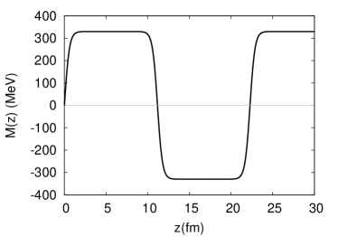
Figure 1: Left: Mass function $M(z)$ for $\Delta=330$ MeV and $\nu=1-10^{-14}$. Right: Corresponding density profile at $T=0$ and $\mu=323.3$ MeV.

As an example, we show in Fig. 1 the mass function for $\Delta=330$ MeV and $\nu=1-10^{-14}$ (left), and the corresponding density profile at $T=0$ and $\mu=323.3$ MeV (right). Comparing these figures, one can see that the density is peaked at the points where the mass functions vanish, i.e., the regions of high density correspond to the regions where chiral symmetry is almost restored. This is reminiscent of the bag model, where the quarks are only allowed in the trivial vacuum.

Because of the alternating sign of the mass function, the density peaks could be identified with solitons and antisolitons when projected onto one spatial dimension parallel to the $z$-axis. In $3+1$ dimensions, this distinction is not well defined because the domain-walls can be oriented in any direction so that “solitons” and “antisolitons” are connected by a continuous transformation. In any case, as obvious from Eq. (11), the density does not depend on the sign of the mass function. Therefore the distance $a$ between two neighboring peaks is equal to one half of the period $L$, where $L$ is given in Eq. (3),

$$a=\frac{L}{2}=\frac{{\bf K}(\nu)}{\Delta}\,.$$ (12)

II.3 Single-soliton limit

In the limit $\nu\rightarrow 1$, the period $L$ goes to infinity, and the mass function, Eq. (2), features a single kink at $z=0$,

$$M(z)|_{\nu=1}=\Delta\,\tanh(\Delta z)\,,$$ (13)

corresponding to a single soliton. The density of states, Eq. (II.1), becomes

$${\rho}_{\mathit{inh}}(E;\Delta,\nu=1)\,=\,\theta(E-\Delta)\,\frac{1}{\pi^{2}}E\sqrt{E^{2}-\Delta^{2}}\,\equiv\,{\rho}_{\mathit{hom}}(E;\Delta)\,,$$ (14)

which is equal to the density of states of an ideal gas of quarks with constant mass $\Delta$. As a consequence, the free energy of the inhomogeneous phase in the single-soliton limit becomes degenerate with the free energy of homogeneous matter with a constituent quark mass $\Delta$.

For the density matrix element Eq. (11) one gets

$$\rho_{\mathit{D,inh}}(E,z;\Delta,\nu=1)=\rho_{\mathit{hom}}(E;\Delta)+\rho_{\mathit{D,sol}}(E,z;\Delta)\,,$$ (15)

with a localized part

$$\rho_{\mathit{D,sol}}(E,z;\Delta)=\frac{E\Delta}{4\pi}\,\left(\theta(\Delta-E)+\theta(E-\Delta)\frac{2}{\pi}\arcsin{\frac{\Delta}{E}}\right)\,\frac{1}{\cosh^{2}(\Delta z)}$$ (16)

and a homogeneous background given by Eq. (14). The latter is again equal to the analogous term in homogeneous matter.

Accordingly, the density one obtains from Eq. (9) can be separated into a constant background, which is equal to the density in a homogeneous ideal gas of quarks with mass $\Delta$ at given temperature and chemical potential, and a localized peak, which corresponds to the extra quarks in the solitons. In particular, since the localized part drops off exponentially at large values of $|z|$, the average density

$${\bar{n}}=\lim_{L\rightarrow\infty}\frac{1}{2L}\int\limits_{-L}^{L}dz\,n(z)$$ (17)

is entirely determined by the background and, thus, equal to the density in homogeneous matter. As a consequence, a phase transition from the inhomogeneous phase to the homogeneous chirally broken phase taking place at $\nu=1$ is second order.

The additional density contribution due to the quarks in the solitons,

$$n_{\mathit{sol}}(z)=N_{f}N_{c}\int\limits_{0}^{\infty}dE\,\rho_{\mathit{D},sol}(E,z;\Delta)\left(n_{+}(E)-n_{-}(E)\right)\,,$$ (18)

is perhaps the most interesting part. In particular, $n_{\mathit{sol}}(z)$ and, thus, $n(z)$ is nonzero even at $T=0$ and $\mu<\Delta$, when the background density vanishes. In this case, which corresponds to a single soliton embedded in the vacuum, one finds

$$n_{\mathit{sol}}(z)|_{\{\Delta>\mu,T=0\}}\,=\,\frac{N_{f}N_{c}}{8\pi}\frac{\Delta\mu^{2}}{\cosh^{2}(\Delta z)}\,.$$ (19)

Note, however, that here we have simply assumed that solutions with $\nu=1$ and $\Delta>\mu$ exist at zero temperature. Of course, we have to check whether this comes out of the minimization of the thermodynamic potential. Since $\nu=1$ is realized exactly at the second-order phase transition from the homogeneous to the inhomogeneous chirally broken phase, this means that at the critical chemical potential $\mu_{\mathit{c,inh}}$, the amplitude $\Delta$ must be bigger than $\mu_{\mathit{c,inh}}$. On the other hand, at $\mu=\mu_{\mathit{c,inh}}$, the amplitude $\Delta$ is equal to the constituent mass $M$ in the homogeneous phase. Moreover, in the homogeneous chirally broken phase, $M$ remains equal to the vacuum mass $M_{\mathit{vac}}$ as long as $\mu<M_{\mathit{vac}}$. Hence, if at $T=0$ there is a second-order phase transition to the inhomogeneous phase at $\mu_{\mathit{c,inh}}<M_{\mathit{vac}}$, then a single-soliton solution exists at $\mu=\mu_{\mathit{c,inh}}$, with the density profile given by Eq. (19) and $\Delta=M_{\mathit{vac}}$.

In the next section this will be investigated further from the energy-per-particle perspective.

III Energy per particle

Starting from the thermodynamic potential, other thermodynamic quantities can be derived in the usual way, as long as we are only interested in spatial averages. Restricting ourselves to zero temperature, this means that the pressure $p$, the averaged quark number density ${\bar{n}}$ and the averaged energy density ${\bar{\epsilon}}$ are given by

$$p=-(\Omega(\mu)-\Omega_{\mathit{vac}})\,,\qquad{\bar{n}}=\frac{\partial p}{\partial\mu},\qquad{\bar{\epsilon}}=-p+\mu{\bar{n}}\,.$$ (20)

Here $\Omega_{\mathit{vac}}$ is the value of the thermodynamic potential at its minimum in vacuum, which we subtract to define the vacuum pressure to be zero. As a consequence, the energy density of the vacuum vanishes as well. The average energy per quark is then given by

$$\frac{E}{N}=\frac{{\bar{\epsilon}}}{{\bar{n}}}=-\frac{p}{{\bar{n}}}+\mu\,.$$ (21)

In the context of the interpretation of quark droplets as “baryons”, the thermodynamics is often discussed in terms of the baryon number density $\rho_{B}=n/N_{c}$ and the energy per baryon $E/A=N_{c}E/N$, see, e.g., Refs. Buballa:1996tm ; Buballa:1998ky ; Fukushima:2012mz . However, for most quantities we are going to discuss in this article, it is more natural to work with quark number densities and $E/N$. We therefore keep the notation introduced above, noting that the conversion to baryon quantities is simply a factor of $N_{c}=3$. Moreover, in our numerical examples we will scale the densities by $n_{0}=N_{c}\rho_{0}$, so that $n/n_{0}=\rho_{B}/\rho_{0}$. Here $\rho_{0}=0.17$ fm^-3 is the nuclear matter saturation density, i.e., the corresponding quark number density is $n_{0}=0.51$ fm^-3.

From Eq. (21), it follows that the density derivative of $E/N$ is given by

$$\frac{\partial}{\partial{\bar{n}}}\left(\frac{E}{N}\right)=\frac{1}{{\bar{n}}}\left(\mu-\frac{E}{N}\right)=\frac{p}{{\bar{n}}^{2}}\,,$$ (22)

where we have used that $\mu=\partial{\bar{\epsilon}}/\partial{\bar{n}}$ at $T=0$ and fixed volume. For ${\bar{n}}\neq 0$, this means that $E/N$ has an extremum at the points where the pressure vanishes, and it takes the value $E/N=\mu$ at these points.

For ${\bar{n}}\rightarrow 0$, on the other hand, the exact behavior of $E/N$ depends on the density dependence of the pressure. In the case of homogeneous quark matter, the NJL model at low densities behaves like an ideal nonrelativistic gas of constituent quarks, $p\propto n^{5/3}$. Consequently, $E/N$ goes to $\mu$, which in turn converges to the vacuum constituent quark mass $M_{\mathit{vac}}$, while the density derivative of $E/N$ diverges at $n=0$. As we will see below, the behavior of inhomogeneous matter is rather different.

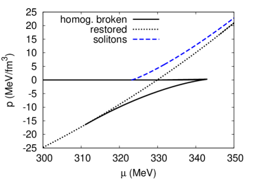
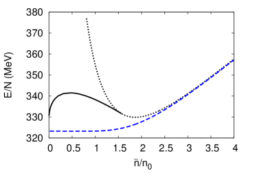
Figure 2: Pressure as function of the chemical potential (left) and energy per quark as a function of the spatially averaged quark number density (right). The homogeneous chirally broken and restored solutions are indicated by the solid and dotted lines, respectively, while the dashed lines indicate the inhomogeneous solitonic solutions.

To this end, we now turn to the numerical results. Our model contains two parameters: the coupling constant $G$ and the Pauli-Villars regulator $\Lambda$. We fix them by fitting the pion decay constant in vacuum to its value in the chiral limit, $f_{\pi}=88$ MeV, and by choosing a reasonable value for the constituent quark mass in vacuum. If not stated otherwise, we choose $M_{\mathit{vac}}=330$ MeV, corresponding to $\Lambda=728.368$ MeV and $G\Lambda^{2}=6.599$.

In the left panel of Fig. 2, we show the pressure as a function of $\mu$. The homogeneous chirally broken solutions are indicated by the solid line, where the upper branch corresponds to the minima of the thermodynamic potential, i.e., to the stable or metastable solutions, while the lower branch corresponds to the maxima, i.e., to the unstable solutions. The chirally restored solutions are indicated by the dotted line. Restricting the analysis to these homogeneous solutions, we find a first-order chiral phase transition at $\mu=\mu_{\mathit{c,hom}}=329.9$ MeV, i.e., slightly below $\mu=M_{\mathit{vac}}$. Accordingly, the energy per particle in the restored phase, indicated by the dotted line in the right panel of Fig. 2, has a minimum with $E/N=\mu_{\mathit{c,hom}}$ at ${\bar{n}}=(2/\pi^{2})\mu_{\mathit{c,hom}}^{3}$, whereas in the homogeneous chirally broken solution (solid line), $E/N$ is always larger, converging to $M_{\mathit{vac}}$ at ${\bar{n}}=0$ with an infinite slope. Thus, in the “old picture”, we would interpret the minimum in the restored phase as a bag-model-like quark droplet with a binding energy per quark of $M_{\mathit{vac}}-\mu_{\mathit{c,hom}}$.

This picture is changed if we allow for the one-dimensional solitonic solutions, as indicated by the dashed lines in Fig. 2. We then find a second-order phase transition from the homogeneous chirally broken phase to the inhomogeneous phase at $\mu=\mu_{\mathit{c,inh}}=323.2$ MeV (left panel). As discussed in Sect. II.3, the inhomogeneous phase at this point corresponds to a single soliton ($\nu=1$) with vanishing background density. Hence, there is no longer a stable solution with zero pressure and nonzero average density, and therefore the only minimum of the energy per particle exists at ${\bar{n}}=0$ (right panel). On the other hand, the localized quarks inside the soliton experience additional binding, so that $E/N$ does not go to $M_{\mathit{vac}}$ at ${\bar{n}}=0$, as for homogeneous matter, but to $\mu_{\mathit{c,inh}}$, which is smaller than $M_{\mathit{vac}}$ in this example. The binding effect is also visible at nonvanishing ${\bar{n}}$. In particular, the chirally restored solution with the minimal $E/N$ is unstable against forming a soliton lattice with the same average density. We find that here the solitons still have a sizable overlap, with density peaks separated by about $a=1.5$ fm. This system can then lower its energy further by expansion.

In this context, a striking difference to the homogeneous case is the fact that the density derivative of $E/N$ does not diverge at ${\bar{n}}=0$ but, on the contrary, the function is extremely flat. According to Eq. (22), this means that the pressure goes to zero with a high power of $n$. Further insight can be obtained from the observation in Ref. Carignano:2010ac that the density rise above the onset of the solitonic phase is consistent with the parametrization

$${\bar{n}}(\mu)=-\frac{c\mu_{\mathit{c,inh}}^{3}}{\ln(\mu/\mu_{\mathit{c,inh}}-1)}\,,$$ (23)

where $c$ is a constant parameter. This formula was motivated by a similar behavior in the Gross-Neveu model. Strictly speaking, it describes the density change $\delta{\bar{n}}$ relative to the density at $\mu=\mu_{\mathit{c,inh}}$. However, since $\mu_{\mathit{c,inh}}<M_{\mathit{vac}}$ in the present case, we have ${\bar{n}}(\mu_{\mathit{c,inh}})=0$ and, hence, $\delta{\bar{n}}={\bar{n}}$. We then find

$$\frac{\partial p}{\partial{\bar{n}}}=\frac{\partial p}{\partial\mu}\left(\frac{\partial{\bar{n}}}{\partial\mu}\right)^{-1}=\frac{c\mu_{\mathit{c,inh}}^{4}}{{\bar{n}}}\,e^{-c\mu_{\mathit{c,inh}}^{3}/{\bar{n}}}\,,$$ (24)

where we have used Eqs. (20) and (23) to evaluate the derivatives. It follows that $\frac{\partial p}{\partial{\bar{n}}}$ is exponentially suppressed for ${\bar{n}}\rightarrow 0$. The same is true for all higher derivatives and all derivatives of $E/N$, thus explaining its flatness. In fact, integrating Eq. (24) to obtain $p({\bar{n}})$ and inverting Eq. (23) for $\mu({\bar{n}})$, we get from Eq. (21) that the energy per particle at low densities should be given by

$$\frac{E}{N}=\mu_{\mathit{c,inh}}\left(1+e^{-c\mu_{\mathit{c,inh}}^{3}/{\bar{n}}}-\frac{c\mu_{\mathit{c,inh}}^{3}}{{\bar{n}}}\int\limits_{c\mu_{\mathit{c,inh}}^{3}/{\bar{n}}}^{\infty}\!\!\!dx\;\frac{e^{-x}}{x}\right)\,.$$ (25)

In Fig. 3, this expression is compared with the numerical results for $E/N$. Fitting the parameters $c$ and $\mu_{c,inh}$ to the data below ${\bar{n}}=n_{0}$ (left), we find a reasonable description up ${\bar{n}}=2n_{0}$ (right), where the increase of $E/N$ is more than a factor of 50 larger. We remark that the fitted value for $c$ is very close to $\mu_{\mathit{c,inh}}/M_{\mathit{vac}}$, but we have not been able to show this analytically.

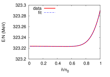
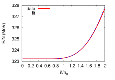
Figure 3: Energy per particle as a function of the average density at $T=0$: numerical results (red solid line) and according to Eq. (25) with $c=0.97985$ and $\mu_{\mathit{c,inh}}=323.223$ MeV (blue dashed line).

For completeness, we also comment on the behavior at high densities. In our example with $M_{\mathit{vac}}=330$ MeV, the system stays inhomogeneous up to arbitrarily high chemical potentials. For somewhat lower values of $M_{\mathit{vac}}$, there is first a second-order phase transition from the solitonic phase to the restored phase, but the system gets inhomogeneous again at higher chemical potentials. As discussed in detail in Ref. Carignano:2011gr , this so-called “inhomogeneous continent” is not a trivial regularization effect, but it cannot be excluded that it is a model artifact. In this article, however, we are mainly interested in the low-density behavior of the model, where this issue is irrelevant.

The results shown in Fig. 2 have been obtained for specific parameters, and one might wonder how robust they are when these are changed. As discussed in Refs. Buballa:2005 ; Buballa:1996tm ; Buballa:1998ky , the binding energy of homogeneous quark matter depends on the amount of scalar attraction, which can be parametrized by $M_{\mathit{vac}}$. In Fig. 4, we therefore show the binding energies per quark in homogeneous matter and in the solitons, $E_{\mathit{b,hom}}=M_{\mathit{vac}}-\mu_{\mathit{c,hom}}$ and $E_{\mathit{b,sol}}=M_{\mathit{vac}}-\mu_{\mathit{c,inh}}$, respectively, as functions of $M_{\mathit{vac}}$.

We see that both curves start at the same point around $M_{\mathit{vac}}=250$ MeV with a negative binding energy. For homogeneous matter, this point corresponds to the limiting case where the phase transition turns from first to second order when $M_{\mathit{vac}}$ is lowered further. In other words, this point corresponds to the case where the tricritical point of the phase boundary in the $T-\mu$ plane is just located at the $T=0$ axis. Since in this model the tricritical point is equal to the Lifshitz point Nickel:2009ke , i.e., the point where the two homogeneous phases and the inhomogeneous phase meet, the binding energies of homogeneous and inhomogeneous matter are equal at this point, and both solutions cease to exist at lower values of $M_{\mathit{vac}}$.

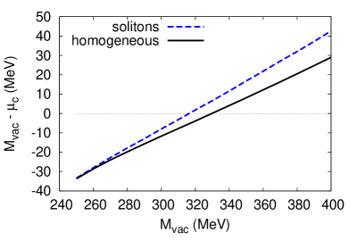
Figure 4: Binding energy per quark for homogeneous matter (solid line) and for solitons (dashed line) as functions of the vacuum constituent quark mass.

When $M_{\mathit{vac}}$ is increased, the binding energies rise. The would-be first-order phase transition from the homogeneous chirally broken to the restored phase is now inside the inhomogeneous regime, i.e., $\mu_{\mathit{c,inh}}<\mu_{\mathit{c,hom}}$ and, hence, $E_{\mathit{b,sol}}>E_{\mathit{b,hom}}$. This means, the chirally restored solution with the lowest $E/N$ is always unstable against forming a soliton lattice.

On the other hand, for $M_{\mathit{vac}}<315$ MeV, $\mu_{\mathit{c,inh}}$ is still smaller than $M_{\mathit{vac}}$. Then the density in the homogeneous chirally broken phase is already nonzero when the phase transition to the inhomogeneous phase takes place. Thus, as discussed in Sec. II.3, the soliton is embedded in a homogeneous background of constituent quarks at this point. As the pressure is nonzero, the system wants to expand. However, since all solutions with a lower average density are homogeneous, this means that the inhomogeneous phase, including the single-soliton solution is not stable without applying external forces. As a consequence, the lowest $E/N$ is obtained for a dilute gas of constituent quarks in the limit of zero density.

For $M_{\mathit{vac}}>315$ MeV, $E_{\mathit{b,sol}}$ is positive, i.e., the lowest $E/N$ corresponds to a single soliton state, as discussed above. For $M_{\mathit{vac}}>330$ MeV, $E_{\mathit{b,hom}}$ is positive as well. So there would be stable droplets of homogeneous matter if we could ignore the possibility of inhomogeneity. As explained above, this is, however, not the case. At $M_{\mathit{vac}}=400$ MeV, for example, the binding energy for homogeneous matter is about 30 MeV per quark, while it is about 40 MeV per quark for the solitons.

For simplicity, all calculations in this article are done in the chiral limit. The mass functions and phase diagrams for non-vanishing bare quark masses have been investigated in Refs. Nickel:2009wj ; Carignano:2010ac , and turned out not to be very different. In particular, the inhomogeneous phase is delimited by second-order phase boundaries, and the mass function at the boundary towards lower $\mu$ takes the form of a single soliton. Therefore, we do not expect our results to change qualitatively if finite bare quark masses are considered.

IV Properties of single solitons

After having explored the conditions for the existence of single self-bound solitons, we would now like to investigate their properties in more details.

As discussed in Sec. II.3, the density profile is given by Eq. (19) with $\mu=\mu_{\mathit{c,inh}}$ and $\Delta=M_{\mathit{vac}}$,

$$n_{\mathit{sol}}(z)\,=\,\frac{N_{f}N_{c}}{8\pi}\frac{M_{\mathit{vac}}\,\mu_{\mathit{c,inh}}^{2}}{\cosh^{2}(M_{\mathit{vac}}\,z)}\,,$$ (26)

where $\mu_{\mathit{c,inh}}<M_{\mathit{vac}}$. We have already noted that $n_{\mathit{sol}}(z)$ decreases exponentially at large $|z|$ and therefore the average density ${\bar{n}}$ vanishes. On the other hand, the central density at $z=0$ is larger than the density of restored quark matter at the same chemical potential,

$$n_{\mathit{sol}}(0)\,=\,\frac{N_{f}N_{c}}{8\pi}\,M_{\mathit{vac}}\,\mu_{\mathit{c,inh}}^{2}\,=\,\frac{3\pi}{8}\frac{M_{\mathit{vac}}}{\mu_{\mathit{c,inh}}}\,n_{\mathit{rest}}\,,$$ (27)

where $n_{\mathit{rest}}=\frac{N_{f}N_{c}}{3\pi^{2}}\,\mu_{\mathit{c,inh}}^{3}$. This can be interpreted as a bag-pressure effect, which pushes the quarks out of the chirally broken vacuum and squeezes them into the restored regions Carignano:2010ac .

The number of quarks in the soliton per transverse area $A_{\perp}$ is obtained by integrating Eq. (26) over $z$. One finds

$$\frac{N}{A_{\perp}}\,=\,\frac{N_{f}N_{c}}{4\pi}\,\mu_{\mathit{c,inh}}^{2}\,.$$ (28)

Another interesting quantity is the longitudinal rms “radius”,

$$R_{\mathit{sol,\parallel}}^{\mathit{rms}}\,\equiv\,\sqrt{\langle{z^{2}}\rangle}\,=\,\left(\frac{\int dz\,z^{2}\,n_{\mathit{sol}}(z)}{\int dz\,n_{\mathit{sol}}(z)}\right)^{1/2}\,=\,\frac{\pi}{\sqrt{12}}\,\frac{1}{M_{\mathit{vac}}}\,,$$ (29)

which is a measure for the half-size of the soliton in $z$-direction.

Similarly, we can define the “soliton averaged density”, i.e., the density-weighted integral over the density divided by the number of quarks,

$$\langle{n}\rangle_{\mathit{sol}}\,=\,\frac{\int dz\,n_{\mathit{sol}}^{2}(z)}{\int dz\,n_{\mathit{sol}}(z)}\,=\,\frac{N_{f}N_{c}}{12\pi}\,M_{\mathit{vac}}\,\mu_{\mathit{c,inh}}^{2}\,.$$ (30)

Hence

$$\langle{n}\rangle_{\mathit{sol}}\,=\,\frac{2}{3}n_{\mathit{sol}}(0)\,=\,\frac{\pi}{4}\frac{M_{\mathit{vac}}}{\mu_{\mathit{c,inh}}}\,n_{\mathit{rest}}\,,$$ (31)

i.e., while the maximal density in a self-bound soliton is always larger than the density in the restored phase at the same chemical potential, $\langle{n}\rangle_{\mathit{sol}}$ can be smaller. For instance, for $M_{\mathit{vac}}=400$ MeV, we have $M_{\mathit{vac}}/\mu_{\mathit{c,inh}}=1.12<4/\pi$.

It is interesting to compare these expressions with the results based on the droplet picture for homogeneous matter. As discussed earlier, the most stable homogeneous solution corresponds to quark matter in the restored phase at the critical chemical potential $\mu_{\mathit{c,hom}}$, provided $\mu_{\mathit{c,hom}}<M_{\mathit{vac}}$. The density is, thus, given by

$$n_{\mathit{hom}}=\frac{N_{f}N_{c}}{3\pi^{2}}\,\mu_{\mathit{c,hom}}^{3}\,.$$ (32)

Assuming that the homogeneous solutions could be taken over to describe small quark matter droplets, the volume of a “baryon” with $N_{c}$ quarks would be $V_{\mathit{hom}}=N_{c}/n_{\mathit{hom}}$. For spherical bags, this would correspond to a radius of

$$R_{\mathit{hom,s}}=\left(\frac{9\pi}{4N_{f}}\right)^{1/3}\,\frac{1}{\mu_{\mathit{c,hom}}}\,,$$ (33)

which turns out to be quite reasonable if the numerical values for $\mu_{\mathit{c,hom}}$ are inserted Buballa:1996tm , see Table 1. However, since the underlying formalism, which assumes infinite matter, does not provide any mechanism why the matter should clusterize and, if so, why into droplets of $N_{c}$ quarks, this description of baryons as quark droplets remains very schematic.

In this sense, the domain-wall solitons, which are finite in one spatial direction, could be seen as a step into the right direction. Moreover, the longitudinal size, given by Eq. (29), turns out to be of the correct order. To illustrate this, we perform a quantitative comparison with the homogeneous “baryon” droplets by again restricting the volume in such a way that it contains $N_{c}$ quarks. Since the longitudinal shape of the soliton is predicted by the model, we want to keep it untouched and only restrict the transverse area by hand. Taking a circular shape, Eq. (28) yields

$$R_{\mathit{sol,\perp}}=\frac{2}{\sqrt{N_{f}}}\,\frac{1}{\mu_{\mathit{c,inh}}}\,.$$ (34)

Of course, the non-spherical geometry of this “baryon” should not be taken seriously, but is simply a consequence of the described procedure. For the sake of a meaningful comparison with the homogeneous droplets, we take the latter to be non-spherical as well, but assume a cylindrical shape. For simplicity, we assume that the transverse and longitudinal radii of the cylinder are equal, i.e., the cylinder has a transverse radius $R_{\mathit{hom,c}}$ and a height $2R_{\mathit{hom,c}}$. Since the volume must remain unchanged, $R_{\mathit{hom,c}}$ is then related to the radius of the sphere by $R_{\mathit{hom,c}}=(2/3)^{1/3}R_{\mathit{hom,s}}$, i.e.,

$$R_{\mathit{hom,c}}=\left(\frac{3\pi}{2N_{f}}\right)^{1/3}\,\frac{1}{\mu_{\mathit{c,hom}}}\,.$$ (35)

Moreover, for better comparability with $R_{\mathit{sol,\parallel}}^{\mathit{rms}}$, we translate all sharp radii into rms radii. For a D-dimensional sphere with radius $R_{i}$, the relation is given by

$$R_{i}^{\mathit{rms}}=\left(\frac{\int d^{D}r\,r^{2}\,\theta(R_{i}-r)}{\int d^{D}r\,\theta(R_{i}-r)}\right)^{1/2}=\sqrt{\frac{D}{D+2}}\,R_{i}\,,$$ (36)

i.e., we have $R_{\mathit{sol,\perp}}^{\mathit{rms}}/R_{\mathit{sol,\perp}}=R_{\mathit{hom,\perp}}^{\mathit{rms}}/R_{\mathit{hom,c}}=1/\sqrt{2}$ and $R_{\mathit{hom,\parallel}}^{\mathit{rms}}/R_{\mathit{hom,c}}=1/\sqrt{3}$.

Finally, we define a “baryon mass” for the homogeneous and solitonic solutions as $N_{c}$ times $E/N$, i.e.,

$$M_{\mathit{B,hom}}=N_{c}\,\mu_{\mathit{c,hom}}\,,\qquad M_{\mathit{B,sol}}=N_{c}\,\mu_{\mathit{c,inh}}\,.$$ (37)

$M_{\mathit{vac}}$ [MeV]	$\mu_{\mathit{c,hom}}$ [MeV]	$M_{\mathit{B,hom}}$ [MeV]	$n_{\mathit{hom}}/n_{0}$	$R_{\mathit{hom,s}}$ [fm]	$R_{\mathit{hom,\perp}}^{\mathit{rms}}$ [fm]	$R_{\mathit{hom,\parallel}}^{\mathit{rms}}$ [fm]
330	329.9	1989.7	1.86	0.91	0.56	0.46
400	371.0	1113.0	2.64	0.81	0.50	0.41

Table 1: Properties of homogeneous “baryon droplets” for two values of the vacuum constituent quark mass $M_{\mathit{vac}}$.

$M_{\mathit{vac}}$ [MeV]	$\mu_{\mathit{c,inh}}$ [MeV]	$M_{\mathit{B,sol}}$ [MeV]	$n_{\mathit{sol}}(0)/n_{0}$	$\langle{n}\rangle_{\mathit{sol}}/n_{0}$	$R_{\mathit{sol,\perp}}$ [fm]	$R_{\mathit{sol,\perp}}^{\mathit{rms}}$ [fm]	$R_{\mathit{sol,\parallel}}^{\mathit{rms}}$ [fm]
330	323.2	1969.7	2.10	1.40	0.86	0.61	0.54
400	357.4	1072.2	3.11	2.08	0.78	0.55	0.45

Table 2: Properties of solitonic “baryons” for two values of the vacuum constituent quark mass $M_{\mathit{vac}}$.

The results for $N_{f}=2$ and $N_{c}=3$ and two different values of $M_{\mathit{vac}}$ are summarized in Table 1 for homogeneous droplets and in Table 2 for the solitons. We find that the qualitative and even the quantitative behavior is similar for both cases. The “baryon masses” rise with the vacuum quark mass, but are below $3M_{\mathit{vac}}$ because of binding effects. Since the binding increases with increasing quark masses, the densities increase as well, while the radii decrease. As discussed in the previous section, the solitons are bound more strongly than homogeneous matter. As a consequence, the solitons have a larger central density, despite the fact that the chemical potential is lower. The soliton averaged density $\langle{n}\rangle_{\mathit{sol}}$, on the other hand, is smaller than the density in homogeneous droplets. Therefore, the solitons have larger rms radii.

Nevertheless, the general agreement of the various rms radii for a given quark mass turns out to be quite good. In particular, it is remarkable that $R_{\mathit{sol,\parallel}}^{\mathit{rms}}$, which is an intrinsic property of the soliton, is similar to the other radii, which have been introduced by hand in order to have three quarks in a “baryon”. On the other hand, the sharp radii $R_{\mathit{hom,s}}$ and $R_{\mathit{sol,\perp}}$ are considerably larger, showing that the numbers are rather sensitive to the used definition of the radius.

V Soliton-soliton interactions

Having discussed the properties of single solitons, we now move away from this limit and investigate what happens when the solitons approach each other.

As explained in Sec. II, the inhomogeneous solutions are characterized by the parameters $\nu$ and $\Delta$, which are obtained by minimizing the thermodynamic potential at given $T$ and $\mu$. In particular the distance $a$ between the neighboring solitons depends on $\nu$ and $\Delta$, as detailed in Eq. (12). This allows us to plot the thermodynamic quantities of the system as functions of $a$, which is sometimes more instructive than plotting them against $\mu$ or ${\bar{n}}$.

As before, we limit ourselves to $T=0$. At the boundary to the homogeneous chirally broken phase, we have $\nu=1$, corresponding to $a\rightarrow\infty$, while with increasing chemical potential the distance quickly becomes smaller. For large distances, the density distribution of the soliton lattice does not differ much from a linear superposition of single solitons. The average density is therefore given by

$${\bar{n}}_{\infty}(a)=\frac{N_{f}N_{c}}{4\pi}\,\frac{\mu_{\mathit{c,inh}}^{2}}{a}\,,$$ (38)

i.e., the column density of a single soliton, Eq. (28), divided by the distance. At smaller distances, on the other hand, the interaction between the solitons leads to nonlinearities, giving rise to deviations from the trivial $1/a$ behavior. This is shown in the upper left panel of Fig. 5, where ${\bar{n}}/{\bar{n}}_{\infty}$ is displayed as a function of $a$. We see that the ratio is very close to unity for $a>2$ fm and rises steeply when the distance is decreased below 1 fm. Here $a$ is smaller than $2R_{\mathit{sol,\parallel}}^{\mathit{rms}}$, i.e., the solitons strongly overlap. A similar picture arises from the energy per particle (upper right) and the pressure (lower left) when plotted as functions of the soliton distance: For $a>2$ fm, $E/N$ is almost independent of $a$ and $p$ remains close to zero, while both quantities rise steeply at $a<1$ fm.

Figure 5: Various quantities as functions of the soliton-soliton distance $a$: ratio of the average density ${\bar{n}}$ and the corresponding value ${\bar{n}}_{\infty}$ for noninteracting solitons, Eq. (38) (upper left), energy per quark (upper right), pressure (lower left), and effective force per quark, Eq. (39) (lower right).

For thin, well separated solitons, the pressure can be interpreted as the force per transverse area by which they repel each other, $F(A_{\perp})=pA_{\perp}$. Dividing this force by the corresponding number of quarks in the soliton, $N(A_{\perp})={\bar{n}}aA_{\perp}$, we obtain the effective force per quark

$$\langle{\frac{F}{N}}\rangle=\frac{p}{{\bar{n}}a}\,,$$ (39)

which is probably the most intuitive way to quantify the soliton-soliton interactions. The resulting behavior as a function of $a$ is shown in the lower right panel of Fig. 5. Again, the “force” vanishes at large distances and becomes nonnegligible only below around 2 fm, when the solitons begin to overlap. Of course, when the overlap gets sizable, the assumption of well separated solitons breaks down and the interpretation as a force must be taken with care.

VI Including vector interactions

It is also interesting to study the influence of vector interactions, which are very important at finite density, as known, e.g., from the Walecka model Walecka:1974qa . In the NJL model with homogeneous condensates, vector interactions have been shown to weaken the first-order chiral phase transition, and already at rather small values of the vector coupling, the phase transition turns into second order or a crossover Buballa:1998ky ; Kitazawa:2002bc ; Fukushima:2008is ; Bratovic:2012qs . In terms of $E/N$, this is easily understood from the fact that the vector interaction, described by a term

$${\cal L}_{V}=-G_{V}(\bar{\psi}\gamma^{\mu}\psi)^{2}$$ (40)

in the Lagrangian, adds a term $G_{V}n^{2}$ to the energy density, i.e., $E/N$ is enhanced by $G_{V}n$ Buballa:1996tm . Hence, the minimum in the restored phase at finite density gets increasingly disfavored with increasing $G_{V}$, whereas the energy at $n=0$ stays unaffected (see Ref. Fukushima:2012mz for a recent general discussion of this point).

The effect of vector interactions on inhomogeneous phases has been investigated in Ref. Carignano:2012sx . In that analysis the approximation was made to replace the density $n(z)$ in the mean-field Lagrangian by the spatial average ${\bar{n}}$. This is a good approximation close to the restored phase and in particular at the Lifshitz point. The shape of the mass function at a given density is then independent of $G_{V}$, and the known analytical solutions for $G_{V}=0$ could basically be taken over. If we could apply the same approximation to our present analysis, we would obtain

$$\left.\frac{E}{N}\right|_{G_{V}}\;\approx\;\left.\frac{E}{N}\right|_{G_{V}=0}\,+\ G_{V}{\bar{n}}\;\equiv\;\left(\frac{E}{N}\right)_{<}\,,$$ (41)

similar to the homogeneous case. This would further stabilize the minimum at ${\bar{n}}=0$.

It is obvious, however, that the replacement of $n$ by ${\bar{n}}$ is not a good approximation at low average densities where the quarks are strongly localized in the solitons and therefore feel a much stronger repulsion than suggested by $G_{V}{\bar{n}}$. For instance, the energy of a single soliton is still enhanced by the vector repulsion, even when the homogeneous background density and, thus, the average density of the system goes to zero. Thus, the correction to $E/N$ should rather be obtained by integrating the local correction to the energy density, $\delta\epsilon(z)=G_{V}n^{2}(z)$ over the volume and divide it by the integrated quark number density. Since the integrals over the transverse area cancel, one obtains

$$\left.\frac{E}{N}\right|_{G_{V}}\;\approx\;\left.\frac{E}{N}\right|_{G_{V}=0}\,+\,G_{V}\frac{\int dz\,n^{2}(z)}{\int dz\,n(z)}\;\equiv\;\left(\frac{E}{N}\right)_{>}\,.$$ (42)

This is still an approximation, at least as long the density profiles $n(z)$ for $G_{V}=0$ which were given in Sec. II.2 are used. We expect that, in a fully self-consistent treatment, the vector repulsion between the quarks leads to a broadening of the density distribution, which lowers the energy. Eq. (42) with the unmodified density profiles should therefore be taken as an upper limit of $E/N$, while Eq. (41) provides a lower limit.

Making use of the periodicity of the soliton lattice, Eq. (42) can be simplified to

$$\left(\frac{E}{N}\right)_{>}\;=\;\left.\frac{E}{N}\right|_{G_{V}=0}\,+\,\frac{G_{V}}{a{\bar{n}}}\int\limits_{0}^{a}dz\,n^{2}(z)\,.$$ (43)

where $a=L/2$ is the distance between the solitons, introduced in Eq. (12). For the single-soliton limit with $\mu_{\mathit{c,inh}}<M_{\mathit{vac}}$, we have $E/N|_{G_{V}=0}=\mu_{\mathit{c,inh}}$, while the integrals in Eq. (42) have readily been worked out in Sec. IV. This yields

$$\left(\frac{E}{N}\right)_{>}\!\!\!({\bar{n}}=0)\;=\;\mu_{\mathit{c,inh}}\,+\,G_{V}\langle{n}\rangle_{\mathit{sol}}\,,$$ (44)

with $\langle{n}\rangle_{\mathit{sol}}$ given in Eq. (30).

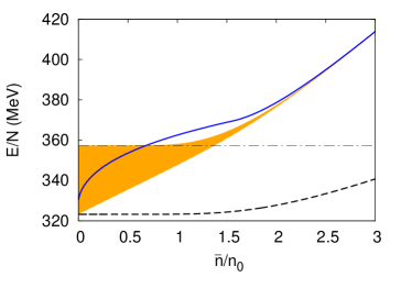
Figure 6: Energy per particle as a function of the average density for a vector coupling $G_{V}=G/2$. The shaded area marks the range between the upper limit Eq. (43) and the lower limit Eq. (41). The ${\bar{n}}=0$-value of the upper limit, Eq. (44), is denoted by the dash-dotted line. Also shown are $E/N$ for homogeneous matter (solid line) and for inhomogeneous matter at $G_{V}=0$ (dashed line).

In Fig. 6 our results for $G_{V}=G/2$ are displayed as functions of the average density. The range between the upper and lower limits of $E/N$ is indicated by the shaded area. For comparison we also show the results for homogeneous matter and for inhomogeneous matter at $G_{V}=0$. One can see that at high densities $(E/N)_{>}$, $(E/N)_{<}$, and $E/N$ for homogeneous matter become practically degenerate. This is not surprising, since in this regime the amplitude $\Delta$ of the mass function becomes small and the density profile gets more and more washed out Carignano:2010ac . At intermediate densities we find the energy of homogeneous matter to be higher than the upper limit of inhomogeneous matter, i.e., the inhomogeneous solution should be favored in this region.

The situation is less clear at lower densities. In the zero-density limit, $(E/N)_{<}$ and $(E/N)_{\mathit{hom}}$ converge against the corresponding limits without vector interactions, i.e., $\mu_{\mathit{c,inh}}$ and $M_{\mathit{vac}}$, respectively, while $(E/N)_{>}$ approaches the value given in Eq. (44). If the vector coupling is sufficiently small,

$$G_{V}<\frac{M_{\mathit{vac}}-\mu_{\mathit{c,inh}}}{\langle{n}\rangle_{\mathit{sol}}}=\frac{12\pi}{N_{f}N_{c}}\frac{1}{\mu_{\mathit{c,inh}}}\left(\frac{1}{\mu_{\mathit{c,inh}}}-\frac{1}{M_{\mathit{vac}}}\right)\,,$$ (45)

the energy of homogeneous matter remains above the upper limit for inhomogeneous matter, even at ${\bar{n}}=0$, i.e., we can be rather sure that the inhomogeneous solutions stay favored. In the present example, however, $G_{V}$ is not so small, and we find the ordering $(E/N)_{<}<(E/N)_{\mathit{hom}}<(E/N)_{>}$ at low densities. If the correct inhomogeneous solution is close to the upper limit, this could mean that the ground state at low densities is homogeneous. On the other hand, it is also possible that the inhomogeneous solution remains favored if the solitons change their size in reaction to the repulsive vector interaction.

VII Conclusions

In this article, we have studied the existence and the properties of self-bound quark matter in the NJL model at zero temperature, focusing on inhomogeneous structures with one-dimensional spatial modulations. The analysis was done in mean-field approximation.

For homogeneous matter, it was found long time ago that the model seems to allow for stable “droplets” of quark matter in the chirally restored phase if the interaction is sufficiently attractive. These droplets have vanishing pressure and a chemical potential lower than the vacuum constituent quark mass, so that they are in mechanical and chemical equilibrium with the vacuum. Related to this, they correspond to a minimum of the energy per particle as a function of density, so that they are stable against homogeneous expansion or collapse. Neglecting finite size effects, this suggests to interpret these solutions as quark bags, and the natural expectation would be that they have a spherical shape if surface effects are taken into account.

Allowing for one-dimensional inhomogeneities, however, it turns out that the homogeneous droplets are unstable against forming a soliton lattice. The solitons repel each other, so that the state with the lowest energy per particle is reached at infinite lattice spacing, corresponding to a vanishing spatially averaged density. Inside the solitons, on the other hand, the density is finite, roughly of the same order as in the homogeneous droplets. Their longitudinal size is about 1 fm, determined by the inverse of the vacuum constituent quark mass. Being one-dimensional objects embedded in the three-dimensional space, the solitons are infinite in the two transverse directions. Thus, taking these results as they are, quark matter at low average density should have a lasagne-like structure, with parallel plates of high densities and voids in between.

At this point, we should ask ourselves how these results can be interpreted. In QCD, we expect that compressed quark matter, when it is released, will expand and finally hadronize. At zero temperature, this means that the matter should split up into baryons, each consisting of $N_{c}$ valence quarks. These baryons may further interact with each other, forming nuclei or nuclear matter, but keep their individuality as separate color-singlet objects.

In the NJL model, the “droplet” solutions found in the analysis of homogeneous quark matter have been suggested to be interpreted as schematic baryons, since they are stabilized by the bag pressure and have a reasonable density. Of course, strictly speaking, these solutions are infinite objects, and a separation into finite baryons would require a negative surface tension Alford:1997zt , while recent analyses suggest that it is positive Molodtsov:2011ii ; Lugones:2011xv ; Pinto:2012aq . From this perspective, the one-dimensional solitons look like a step in the right direction, as they are at least finite in one dimension, where they have a reasonable size. In particular, one might hope that the consideration of higher-dimensional inhomogeneous phases could reveal further instabilities, eventually leading to finite localized baryons as the true ground state of matter at low densities.

Unfortunately, this does not seem to be the case. Phases with two-dimensional modulations have been studied in Ref. Carignano:2012sx and were found to be disfavored against one-dimensional modulations at low densities. Although the analysis was restricted to sinusoidal shapes and certain parameters, it is unlikely that this will change if other shapes or parameters, or even three-dimensional modulations are considered. Nevertheless, more systematic studies in this direction are highly desirable, in particular since at nonzero temperature one-dimensional periodic structures are known to be unstable against fluctuations Landau:1969 ; Baym:1982 . One should also revisit the old works on the chiral quark soliton model Alkofer:1994ph ; Christov:1995vm ; ripka and work out their relation to the present model.

Of course, there is a priori no reason to expect finite baryons to be the most favored objects in a nonconfining model. On the other hand, the model predictions may still have some relevance in the deconfined phase. The emergence of one-dimensional modulations can be understood as a relic of the Peierls instability in $1+1$ dimensions peierls , which is a rather general mechanism. Also the fact that the longitudinal size and the internal density of the one-dimensional solitons are of the order to be expected for baryons might indicate that confinement effects are not very drastic. It is thus conceivable that lasagne-like patterns are preformed in expanding quark matter before hadronization takes place, and it would be interesting to work out possible observable signatures.

The present calculations could also be improved in several aspects: In Sec. VI, we gave only a lower and an upper limit for the effect of vector interactions on the energy per particle. For the upper limit, which is probably closer to the true solution, we assumed that the density profiles remain unchanged when the vector interactions are switched on. However, we expect that the repulsive interaction leads to a broadening of the density peaks, which would lower the energy of the system. In this way the solitons may continuously go over into homogeneous matter, when the vector coupling is increased. We have also neglected the effect of spacelike vector condensates, which should be present in anisotropic systems.

Moreover, we should allow for BCS pairing of the quarks in the solitons. Inside the solitons we find densities of two to three times nuclear-matter density, for which gaps of the order of 50 to 100 MeV have been found in homogeneous quark matter. It would be interesting to see how this is changed for an inhomogeneous environment.

If we want to extend our studies to quark matter in compact stars, we must enforce beta equilibrium and electric neutrality. This would put stress on the present solutions, since the chemical potentials and, hence, the favored periodicities of the soliton lattice would no longer be identical for up and down quarks. If this effect is large, the system may find ways to accommodate different periods, e.g., by forming a two-dimensional lattice, where the up- and down-quark condensates vary independently in different directions. It would also be interesting to include strange quarks and revisit the problem of strange quark matter and strangelets in the NJL model Buballa:1998pr .

Unfortunately, these improvements of the model can no longer be done by making use of the analytically known solutions of the $1+1$ dimensional Gross-Neveu model, so that brute-force numerical diagonalizations of the Hamiltonian seem to be unavoidable.

Finally, we should also include fluctuations. An interesting scenario would be that they leave the inhomogeneous phase (potentially with a higher-dimensional structure) intact but turn the second-order phase transition from the vacuum phase into first order. The minimum of $E/N$ would then be shifted to nonvanishing average density. The resulting crystal could be a first step towards nuclear matter.

References

- (1) Y. Nambu and G. Jona-Lasinio, Phys. Rev. 122, 345 (1961); Phys. Rev. 124, 246 (1961).
- (2) U. Vogl and W. Weise, Prog. Part. Nucl. Phys. 27, 195 (1991).
- (3) S. P. Klevansky, Rev. Mod. Phys. 64, 649 (1992).
- (4) T. Hatsuda and T. Kunihiro, Phys. Rept. 247, 221 (1994) [arXiv:hep-ph/9401310].
- (5) M. Buballa, Phys. Rept. 407, 205 (2005) [arXiv:hep-ph/0402234].
- (6) A. Chodos, R. L. Jaffe, K. Johnson, C. B. Thorn and V. F. Weisskopf, Phys. Rev. D 9, 3471 (1974); A. Chodos, R. L. Jaffe, K. Johnson and C. B. Thorn, Phys. Rev. D 10, 2599 (1974); T. A. DeGrand, R. L. Jaffe, K. Johnson and J. E. Kiskis, Phys. Rev. D 12, 2060 (1975).
- (7) M. Buballa, Nucl. Phys. A 611, 393 (1996) [nucl-th/9609044].
- (8) M. G. Alford, K. Rajagopal and F. Wilczek, Phys. Lett. B 422, 247 (1998) [hep-ph/9711395].
- (9) M. Buballa and M. Oertel, Nucl. Phys. A 642, 39 (1998) [hep-ph/9807422].
- (10) S. V. Molodtsov and G. M. Zinovjev, Phys. Rev. D 84, 036011 (2011) [arXiv:1103.3351 [hep-ph]].
- (11) G. Lugones and A. G. Grunfeld, Phys. Rev. D 84, 085003 (2011) [arXiv:1105.3992 [astro-ph.SR]].
- (12) M. B. Pinto, V. Koch and J. Randrup, arXiv:1207.5186 [hep-ph].
- (13) M. Sadzikowski and W. Broniowski, Phys. Lett. B 488, 63 (2000) [hep-ph/0003282].
- (14) E. Nakano and T. Tatsumi, Phys. Rev. D 71, 114006 (2005) [hep-ph/0411350].
- (15) D. Nickel, Phys. Rev. D 80, 074025 (2009) [arXiv:0906.5295 [hep-ph]].
- (16) S. Carignano, D. Nickel and M. Buballa, Phys. Rev. D 82, 054009 (2010) [arXiv:1007.1397 [hep-ph]].
- (17) S. Carignano and M. Buballa, arXiv:1203.5343 [hep-ph].
- (18) H. Abuki, D. Ishibashi and K. Suzuki, Phys. Rev. D 85, 074002 (2012) [arXiv:1109.1615 [hep-ph]].
- (19) O. Schnetz, M. Thies and K. Urlichs, Annals Phys. 314, 425 (2004) [hep-th/0402014].
- (20) K. Fukushima, arXiv:1204.0594 [hep-ph].
- (21) S. Carignano and M. Buballa, arXiv:1111.4400 [hep-ph].
- (22) D. Nickel, Phys. Rev. Lett. 103, 072301 (2009) [arXiv:0902.1778 [hep-ph]].
- (23) J. D. Walecka, Annals Phys. 83, 491 (1974).
- (24) M. Kitazawa, T. Koide, T. Kunihiro and Y. Nemoto, Prog. Theor. Phys. 108, 929 (2002) [hep-ph/0207255, hep-ph/0307278].
- (25) K. Fukushima, Phys. Rev. D 78, 114019 (2008) [arXiv:0809.3080 [hep-ph]].
- (26) N. M. Bratovic, T. Hatsuda and W. Weise, arXiv:1204.3788 [hep-ph].
- (27) L. D. Landau and E. M. Lifshitz, Statistical physics (Addison-Wesley, Reading, Mass., 1969)
- (28) G. Baym, B. L. Friman and G. Grinstein, Nucl. Phys. B 210, 193 (1982)
- (29) R. Alkofer, H. Reinhardt and H. Weigel, Phys. Rept. 265, 139 (1996) [hep-ph/9501213].
- (30) C. .V. Christov, A. Blotz, H. -C. Kim, P. Pobylitsa, T. Watabe, T. Meissner, E. Ruiz Arriola and K. Goeke, Prog. Part. Nucl. Phys. 37, 91 (1996) [hep-ph/9604441].
- (31) G. Ripka, Quarks bound by chiral fields, Clarendon Press, Oxford 1997.
- (32) R. E. Peierls, Quantum theory of solids, Clarendon Press, Oxford 1955.
- (33) M. Buballa and M. Oertel, Phys. Lett. B 457, 261 (1999) [hep-ph/9810529].