Mode identification in the high-amplitude $\delta$ Scuti star V2367 Cyg

Abstract

We report on a multi-site photometric campaign on the high-amplitude $\delta$ Scuti star V2367 Cyg in order to determine the pulsation modes. We also used high-dispersion spectroscopy to estimate the stellar parameters and projected rotational velocity. Time series multicolour photometry was obtained during a 98-d interval from five different sites. These data were used together with model atmospheres and non-adiabatic pulsation models to identify the spherical harmonic degree of the three independent frequencies of highest amplitude as well as the first two harmonics of the dominant mode. This was accomplished by matching the observed relative light amplitudes and phases in different wavebands with those computed by the models. In general, our results support the assumed mode identifications in a previous analysis of Kepler data.

1 Introduction

The high-amplitude delta Scuti (HADS) stars are defined as $\delta$ Sct stars with peak-to-peak light amplitudes in excess of about 0.3 mag. This amplitude limit is an arbitrary one and there is no other physically identifiably distinction between HADS and other $\delta$ Sct stars. The HADS stars rotate more slowly than other $\delta$ Sct stars with projected rotationally velocities $v\sin i<30$ km s^-1. They pulsate in one or two dominant modes which are generally assumed to be radial modes, but when observed with greater precision from space many more modes are visible. A large number of combination frequencies and harmonics involving the modes of highest amplitude are usually present. The pulsational behaviour of HADS stars seems to be intermediate between that of multimode $\delta$ Scuti stars and Cepheids (Breger, 2007). In fact, first-overtone classical Cepheids and HADS stars follow the same period – luminosity relation with no discontinuity (Soszynski et al., 2008).

The reason why $\delta$ Sct stars pulsate in many nonradial modes while the more massive Cepheids pulsate only in radial modes is due to the behaviour of nonradial pulsation modes in the stellar interior. In the deep interior of an evolved giant star such as a HADS star or low-mass Cepheid, nonradial p modes behave like high-order g modes. As the stellar mass increases, these modes develop an increasingly large number of spatial oscillations which leads to increased radiative damping. Therefore we find fewer and fewer nonradial modes in HADS stars of increasing mass until only radial modes are present in what we then call a Cepheid (Dziembowski, 1977). Indeed, observations suggest that there is a group of HADS which pulsate just in the fundamental and first overtone modes with no nonradial modes (Poretti et al., 2005) (they might be called low-mass Cepheids). While this seems to be the main reason why Cepheids do not pulsate in nonradial modes, it may not be the only reason and the problem needs further investigation (Mulet-Marquis et al., 2007).

The study of HADS stars is important because it is an interesting laboratory for investigating mode interaction and nonlinear behaviour as exemplified by the presence of combination frequencies. The use of combination frequencies for mode identification is well-known in pure g-mode pulsators such as the ZZ Ceti stars (Wu, 2001; Yeates et al., 2005; Montgomery, 2005). Balona (2012) has recently investigated the problem in pulsating main sequence stars. While in ZZ Ceti stars the combination frequencies arise from interactions in a convective zone in which certain approximations are valid, this is not the case in HADS and it turns out that combination frequencies cannot be used for mode identification.

Mode identification is crucial for extracting stellar parameters from the pulsations. The assumption that the modes of highest amplitude in HADS are radial is based on the fact that when two dominant modes are present, their period ratio often agrees with the expected period ratio for first overtone to fundamental radial mode, $P_{1}/P_{0}$, which is in the range 0.77–0.78. The Petersen diagram (Petersen, 1973), which is a plot of $P_{1}/P_{0}$ as a function of $P_{0}$, is very useful for diagnostic purposes. This ratio varies due to rotation with chemical composition (Poretti et al., 2005) and by coupling with the nearby quadrupole mode (Suárez et al., 2006, 2007). The calculated period ratio is also sensitive to the opacity (Lenz et al., 2008).

Table 1: Information on the photometric multisite campaign. EUO: Ege University Observatory; BNAO-Rozhen: Bulgarian National Astronomical Observatory-Rozhen; OAVdA: The Astronomical Observatory of the Autonomous Region of the Aosta Valley; SPM: Observatorio de San Pedro Mártír; RBO: Red Butte Observatory. Telescope apertures are in m. The total number of nights observed and the start end ending Julian dates of the observations relative to JD 24455000 are given.

Observatory	Site	Tel.	CCD
BNAO-Rozhen	Bulgaria	0.60	FLI PL9000
OAVdA	Italy	0.81	FLI PL3041-1-BB
SPM	Mexico	0.84	FLI Fairchild F3041
EUO	Turkey	0.40	Apogee Alta-U47
RBO	USA	0.60	Apogee Alta E47-UV
Observatory	Filters	Dates	Nights
BNAO-Rozhen	${\rm UBVRI}$	2	736.34–737.54
OAVdA	${\rm BVRI}$	3	737.37–739.56
SPM	${\rm UBVR_{c}I_{c}}$	6	718.76–732.98
EUO	${\rm BVRI}$	17	736.29–816.52
RBO	${\rm UBVRI}$	1	741.68–741.93

V2367 Cyg (KIC 9408694) was discovered in a ROTSE survey (Akerlof et al., 2000) and confirmed as a HADS star by Jin et al. (2003) and Pigulski et al. (2009). The star has been observed by the Kepler satellite and recently analyzed by Balona et al. (2012). The light curve is dominated by a single frequency $f_{1}=5.6611$ d^-1 of high amplitude. Two other independent modes with $f_{2}=7.1490$ d^-1 and $f_{3}=7.7756$ d^-1 have amplitudes an order of magnitude smaller than $f_{1}$. Nearly all the light variation is due to these three modes, harmonics of $f_{1}$ and combination frequencies with $f_{1}$, although several hundred other frequencies of very low amplitude are also present in the Kepler photometry.

The star has a much higher projected rotational velocity ($v\sin i=100\pm 10$ km s^-1, Balona et al. (2012)) than other HADS stars, which makes it unusual. Such a large rotational velocity complicates the analysis and increases the likelihood of mode interaction. The ratio $f_{1}/f_{2}=0.792$ is within the expected ratio of second- to first-overtone radial periods which is in the range 0.79–0.80. Balona et al. (2012) attempted to model the observed frequencies as radial modes without mode interaction, but were not successful. A model with mode interaction was found in which $f_{1}$ is identified as the fundamental radial mode and $f_{2}$ the first overtone radial mode coupled with a nearby quadrupole mode.

Considering the complex nature of the pulsation, the question arises as to whether the modes $f_{1}$ and $f_{2}$ are indeed radial and coupled modes as suggested by the models. The model proposed by Balona et al. (2012) would be greatly strengthened if independent mode identification could be made. Since the star is sufficiently bright and of high amplitude, multicolour photometry can be used to provide this verification. The purpose of this paper is to describe a multi-site photometric and spectroscopic campaign on V2367 Cyg and subsequent analysis of mode identification.

2 Spectroscopy

The spectra were used to estimate the stellar atmospheric parameters and the projected rotational velocity, $v\,\sin\,i$. The spectroscopic observations were carried out with two instruments. The Coudè spectra were obtained with the 2-m RCC telescope of the Bulgarian National Astronomical Observatory, Rozhen. We observed the star during the night of 2011 July 27 in three spectral regions: 4770–4970 Å, 4400–4600 Å, and 5090–5290 Å. These three regions contain the H$\beta$ line, Mg II $\lambda$ 4481 Å and a region rich in Fe lines. The instrument uses a Photometrics AT200 camera with a SITe SI003AB $1024\times 1024$ CCD, ($24\,\mu{\rm m}$ pixels) giving a typical resolution R = 16 000 and S/N ratio of about 40. The exposure time was 1200 s. The instrumental profile was checked by using the arc spectrum giving a full width at half maximum (FWHM) of about 0.4 Å. IRAF standard procedures were used for bias subtracting, flat-fielding and wavelength calibration. The final spectra were corrected to the heliocentric wavelengths.

We also obtained spectra with the WIRO longslit spectrograph which uses an e2V 2048² CCD as the detector. An 1800 lines mm^-1 grating in first order yielded a spectral resolution of 1.5 Å near 5800 Å with a 1.2″$\times$ 100″slit. The spectral coverage was 5250–6750 Å. Individual exposure times were 600 s. Reductions followed standard longslit techniques. Multiple exposures were combined yielding final S/N ratios typically in excess of 60 near 5800 Å. Final spectra were Doppler corrected to the heliocentric frame. Each spectrum was then shifted by a small additional amount in velocity so that the Na I D $\lambda\lambda$ 5890, 5996 lines were registered with the mean Na I line wavelength across the ensemble of observations. This zero-point correction to each observation is needed to account for effects of image wander in the dispersion direction when the stellar FWHM of the point spread function was appreciably less than the slit width. Because of these inevitable slit-placement effects on the resulting wavelength solutions at the level of $\leq$10 km s^-1, radial velocity standards were not routinely taken.

3 Atmospheric parameters

Model atmospheres were calculated using the ATLAS 12 code. The VALD atomic line database (Kupka et al., 1999), which uses data from Kurucz (1993), was used to create a line list for the synthetic spectrum. Synthetic spectra were generated using the SYNSPEC code (Hubeny et al., 1994; Krtička, 1998). We adopted a microturbulence of 2 km s^-1. The computed spectrum was convolved with the instrumental profile (Gaussian of 0.4 Å FWHM for the Coudè spectra and 1.5 Å FWHM for the WIRO spectra respectively) and rotationally broadened to fit the observed spectrum under the assumption of uniform rotation.

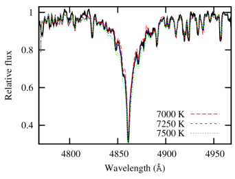
Figure 1: The H$\beta$ line fitted with a model with $T_{\rm eff}=7250~{}{\rm K}$, $\log g=3.5$ (cgs) (short dashes). Two other models with $T_{\rm eff}=7000~{}{\rm K}$ (long dashes) and $T_{\rm eff}=7500~{}{\rm K}$ (dots) are given for comparison.

The best fit to the H$\beta$ and H$\alpha$ lines was obtained for effective temperature $T_{\rm eff}=7250~{}{\rm K}$, and surface gravity $\log g=3.5$. We used the Mg II $\lambda$ 4481 Å line to determine the projected rotational velocity. The best match was obtained with $v\,\sin\,i=90~{}{\rm km\,s^{-1}}$. In Fig. 1 we show the best fit to H$\beta$ as well as the fit using two other models with different temperatures for comparison. Our results for the atmospheric parameters and $v\sin\,i$ are in very good agreement with the results given by Balona et al. (2012) who find $T_{\rm eff}=7300\pm 150$ K, $\log g=3.5\pm 0.1$, $v\sin i=100\pm 10$ km s^-1. Uytterhoeven et al. (2011) list the effective temperature as $T_{\rm eff}=6810\pm 130$ K, which is in disagreement with the above values.

4 Photometry

The photometric data were used to determine the amplitude-colour relation and hence the mode for each frequency.The multi-site photometric campaign on V2367 Cyg was carried out during 2011 June to 2011 September (Julian dates 2455726.69 – 2455816.52) in Europe and North America with five different sites. Although time allocation for 10 d at KISO Observatory, Japan was allocated, no photometric data could be obtained due to bad weather. The time of these observations coincide with Kepler quarter Q9.3–Q10.3. There are over 127780 short-cadence (1 min) Kepler data points in this time range. Table 1 summarizes the sites, telescopes and additional information regarding the campaign.

Since the aim of this campaign is mode identification, multi-colour ${\rm UBVRI}$ filters were chosen. However, EUO and OAVdA do not have the U filter. The U filter, when it is used, leads to high signal-to-noise owing to the poor sensitivity of the CCDs in this wavelength and is therefore not reliable. In any case only four nights of $U$ photometry are available which is not sufficient to resolve the frequencies. Although we show the $U$ observations in mode identification, they should be given very low weight or ignored. All R and I filters are of the Johnson/Bessel type except those at SPM (Mexico) which are of the Cousins/Kron type. The difference is of little consequence as it has a negligible effect on the amplitude ratio and phase difference which are used for mode identification.

When the campaign was initiated in 2011 June, all sites observed the target for 3–4 nights. Subsequently, only EUO continued to observe the target in July, August and early September. A total of 181 hours were spent on observing V2367 Cyg within the 98-d duration of the campaign. Data were reduced using standard IRAF routines including correction for dark, bias and flat-fielding of each CCD frame. The DAOPHOT II package (Stetson, 1987) was used for aperture photometry. The observing times were converted to heliocentric Julian Date (HJD).

Since Kepler photometry was available, it was easy to check the variability of nearby stars. We used the comparison stars GSC 3556  1047 (C1), GSC 3556 1343 (C2) and GSC 3556 627 (C3) because they showed least variability in the Kepler photometry (not more than 50 ppm). Because not all instruments have the same field of view, C2 was not observed by some sites and C1 was chosen as the primary comparison star. The data was therefore reduced relative to C1. Outliers produced by poor seeing or transparency variations were removed by visual inspection.

The passbands of corresponding filters in the instruments on different sites are not exactly the same and neither are the optical characteristics of the instruments. Therefore there are invariably zero-point differences in each filter for each site. Fortunately, we know the frequency composition of the variations in V2367 Cyg from the analysis of the Kepler data by Balona et al. (2012). We can assume that the light variations are well modeled by a Fourier series comprising these frequencies where the zero point will vary from site to site. This is easy to do by fitting the following function to the data by least squares:

$$y_{i}+\epsilon_{i}=\sum_{j=1}^{s}\delta_{ij}a_{j}+\sum_{k=1}^{m}A_{k}\sin(2\pi f_{k}t_{i}+\phi_{k})$$ (1)

where $y_{i}$ is the magnitude at time $t_{i}$ and $\epsilon_{i}$ is the unknown observational error. The number of different sites is $s$ and $\delta_{ij}=0$ unless the $i$-th observation is from site $j$, in which case $\delta_{ij}=1$. The last term is a truncated Fourier series with $m$ frequencies which represents the variability of V2367 Cyg. By minimizing $\sum\epsilon^{2}_{i}$ for $1\leq i\leq N$ ($N$ being the total number of observations), the individual zero points for each site, $a_{j}$, and the amplitudes and phases of the Fourier series can be found.

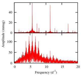
Figure 2: Bottom panel: periodogram of the ground-based $V$ observations of V2367 Cyg. Top panel: periodogram of the Kepler observations over the same time interval.

In Fig. 2 we show the periodogram of the $V$ observations and also of the Kepler observations over the same time interval (JD 2455718.0–2455817.0). The huge advantage of an uninterrupted time series is very clear in this figure.

Table 2: Amplitudes, $A$ (mmag), and phases $\phi$ (radians) for the three frequencies of highest amplitude: $f_{1}=5.66106$, $f_{2}=7.14895$, $f_{3}=7.77557$ d^-1 and harmonics of $f_{1}$. The epoch of phase zero is JD 2455700.000.

Freq	$A$	$\phi$
	$U$
$f_{1}$	$248.9\pm 1.5$	$2.3343\pm 0.0060$
$2f_{1}$	$77.5\pm 1.4$	$2.5586\pm 0.0177$
$f_{2}$	$24.0\pm 1.4$	$-0.5104\pm 0.0586$
$3f_{1}$	$24.7\pm 1.4$	$2.7732\pm 0.0551$
$f_{3}$	$11.9\pm 1.5$	$-0.7500\pm 0.1249$
$4f_{1}$	$12.5\pm 1.4$	$2.6230\pm 0.1090$
	$B$
$f_{1}$	$243.4\pm 1.1$	$2.2941\pm 0.0043$
$2f_{1}$	$75.2\pm 1.0$	$2.4873\pm 0.0140$
$f_{2}$	$26.5\pm 1.1$	$-0.5388\pm 0.0403$
$3f_{1}$	$22.4\pm 1.0$	$2.7301\pm 0.0467$
$f_{3}$	$15.1\pm 1.1$	$-0.7942\pm 0.0706$
$4f_{1}$	$11.4\pm 1.0$	$2.7762\pm 0.0918$
	$V$
$f_{1}$	$186.9\pm 0.7$	$2.2641\pm 0.0035$
$2f_{1}$	$55.1\pm 0.6$	$2.4618\pm 0.0117$
$f_{2}$	$19.4\pm 0.7$	$-0.4727\pm 0.0351$
$3f_{1}$	$16.0\pm 0.6$	$2.7474\pm 0.0401$
$f_{3}$	$10.8\pm 0.7$	$-0.7081\pm 0.0623$
$4f_{1}$	$7.9\pm 0.6$	$2.7543\pm 0.0806$
	$R$
$f_{1}$	$141.7\pm 0.7$	$2.2406\pm 0.0050$
$2f_{1}$	$44.9\pm 0.7$	$2.4660\pm 0.0155$
$f_{2}$	$17.3\pm 0.7$	$-0.3476\pm 0.0407$
$3f_{1}$	$13.6\pm 0.7$	$2.8603\pm 0.0516$
$f_{3}$	$9.5\pm 0.7$	$-0.5988\pm 0.0746$
$4f_{1}$	$6.2\pm 0.7$	$2.6144\pm 0.1124$
	$I$
$f_{1}$	$113.0\pm 0.6$	$2.1942\pm 0.0055$
$2f_{1}$	$36.2\pm 0.6$	$2.4433\pm 0.0169$
$f_{2}$	$13.7\pm 0.6$	$-0.4963\pm 0.0449$
$3f_{1}$	$10.6\pm 0.6$	$2.8294\pm 0.0579$
$f_{3}$	$8.3\pm 0.6$	$-0.6936\pm 0.0746$
$4f_{1}$	$5.3\pm 0.6$	$2.6109\pm 0.1147$

Table 3: Amplitude ratios, $A/A_{B}$, and phase differences $\phi-\phi_{B}$ (radians) relative to the $B$ band for six frequencies of highest amplitude: $f_{1}=5.66106$, $f_{2}=7.14895$, $f_{3}=7.77557$ d^-1.

Filt	$A/A_{B}$	$\phi-\phi_{B}$
	$f_{1}$
$U$	$1.0226\pm 0.0077$	$0.0402\pm 0.0074$
$B$	$1.0000\pm 0.0064$	$0.0000\pm 0.0061$
$V$	$0.7679\pm 0.0045$	$-0.0300\pm 0.0055$
$R$	$0.5822\pm 0.0039$	$-0.0535\pm 0.0066$
$I$	$0.4643\pm 0.0032$	$-0.0999\pm 0.0070$
	$2f_{1}$
$U$	$1.0306\pm 0.0231$	$0.0713\pm 0.0226$
$B$	$1.0000\pm 0.0188$	$0.0000\pm 0.0198$
$V$	$0.7327\pm 0.0126$	$-0.0255\pm 0.0182$
$R$	$0.5971\pm 0.0122$	$-0.0213\pm 0.0209$
$I$	$0.4814\pm 0.0102$	$-0.0440\pm 0.0219$
	$f_{2}$
$U$	$0.9057\pm 0.0648$	$0.0284\pm 0.0711$
$B$	$1.0000\pm 0.0587$	$0.0000\pm 0.0570$
$V$	$0.7321\pm 0.0403$	$0.0661\pm 0.0534$
$R$	$0.6528\pm 0.0378$	$0.1912\pm 0.0573$
$I$	$0.5170\pm 0.0312$	$0.0425\pm 0.0603$
	$3f_{1}$
$U$	$1.1027\pm 0.0796$	$0.0431\pm 0.0722$
$B$	$1.0000\pm 0.0631$	$0.0000\pm 0.0660$
$V$	$0.7143\pm 0.0416$	$0.0173\pm 0.0616$
$R$	$0.6071\pm 0.0414$	$0.1302\pm 0.0696$
$I$	$0.4732\pm 0.0341$	$0.0993\pm 0.0744$
	$f_{3}$
$U$	$0.7881\pm 0.1147$	$0.0442\pm 0.1435$
$B$	$1.0000\pm 0.1030$	$0.0000\pm 0.0998$
$V$	$0.7152\pm 0.0697$	$0.0861\pm 0.0942$
$R$	$0.6291\pm 0.0652$	$0.1954\pm 0.1027$
$I$	$0.5497\pm 0.0564$	$0.1006\pm 0.1027$
	$4f_{1}$
$U$	$1.0965\pm 0.1560$	$-0.1532\pm 0.1425$
$B$	$1.0000\pm 0.1241$	$0.0000\pm 0.1298$
$V$	$0.6930\pm 0.0804$	$-0.0219\pm 0.1222$
$R$	$0.5439\pm 0.0778$	$-0.1618\pm 0.1451$
$I$	$0.4649\pm 0.0666$	$-0.1653\pm 0.1469$

Table 4: Zero points in the ${\rm UBVRI}$ filters for various sites and the number of observations, $N$.

Site	$U$	$N$
Mexico	$-0.078\pm 0.001$	$448$
USA	$-0.033\pm 0.003$	$44$
Site	$B$	$N$	$V$	$N$
Bulgaria	$-0.193\pm 0.003$	$220$	$-0.079\pm 0.002$	$221$
Italy	$-0.210\pm 0.002$	$372$	$-0.120\pm 0.002$	$412$
Mexico	$-0.170\pm 0.001$	$1319$	$-0.081\pm 0.001$	$2152$
Turkey	$-0.205\pm 0.001$	$1955$	$-0.121\pm 0.001$	$2128$
USA	$-0.170\pm 0.007$	$50$	$-0.066\pm 0.005$	$49$
Site	$R$	$N$	$I$	$N$
Bulgaria	$-0.007\pm 0.002$	$220$	$0.075\pm 0.002$	$220$
Italy	$-0.037\pm 0.001$	$410$	$0.056\pm 0.001$	$399$
Mexico	$0.091\pm 0.001$	$395$	$0.092\pm 0.001$	$375$
Turkey	$-0.057\pm 0.001$	$2052$	$-0.002\pm 0.001$	$2008$
USA	$0.013\pm 0.004$	$50$	$0.092\pm 0.004$	$46$

We used the first three independent frequencies of highest amplitude obtained by the frequency extraction described in Balona et al. (2012): $f_{1}=5.661058$, $f_{2}=7.148949$ and $f_{3}=7.775566$ d^-1 together with the first three harmonics of $f_{1}$ ($2f_{1},3f_{1},4f_{1}$) for the least squares Fourier fit (Eq.1). Fitting with these six frequencies does not adequately describe the full variation of the star, but is sufficient to determine the zero points of different sites (Table 4) together with the amplitudes and phases of these particular six frequencies (Table 2). It is these amplitudes and phases which are used in mode identification. Differential $V$-band photometry from all sites adjusted for zero-point differences are shown in Fig. 5. Also shown is the fitted Fourier curve using the six frequencies. From the amplitudes and phases of the fitted Fourier frequency components, we find amplitude ratios and phase differences listed in Table. 3 and shown in Fig. 3.

The harmonics of the principal frequency, $f_{1}$, have large amplitudes and can be used as additional data for mode identification. In fact, the amplitude ratios and phase differences for the harmonics $2f_{1},3f_{1}$, are exactly the same as for the fundamental, $f_{1}$, as can be seen in Fig. 4.

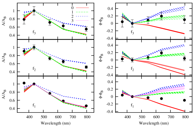
Figure 3: Amplitude ratios (left panels) and phase differences (radians, right panels) for $f_{1},f_{2}$ and $f_{3}$. The curves are from models with a range of stellar parameters of the best estimated values with a range of stellar parameters of $7200<T_{\rm eff}<7400$ K and $3.3<\log g<3.7$, and for different spherical harmonic degrees, $l$($0<l<3$).

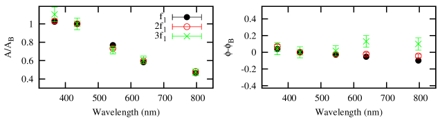
Figure 4: Amplitude ratios (left panel) and phase differences (radians, right panel) for $f_{1}$ and its harmonics, $2f_{1},3f_{1}$.

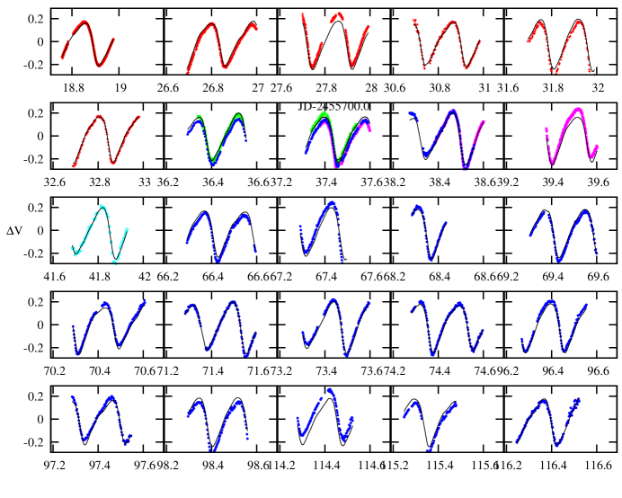
Figure 5: Light curves corrected for zero points showing fitted Fourier curve.

5 Mode identification

There are several techniques that can be used to discriminate between different values of the spherical harmonic degree, $l$. In the simplest technique, the amplitudes ratios relative to a given waveband are compared with the calculated amplitudes ratios. The method relies on the fact that the variation of light amplitude in different wavelength bands depends on $l$ and is independent of the azimuthal number $m$. It should be noted that our current models for photometric mode identification are only valid in the limit of no rotation. Rotation introduces departures from pure spherical harmonics so that a single value of $l$ is not sufficient to describe the eigenfunction perfectly. However, so long as the rotation is not very rapid, a single value of $l$ is still a reasonable approximation. We expect that for V2367 Cyg this will be the case, but the relative amplitudes will be modified to some degree due to this effect.

The most general expression for the magnitude variation, $m_{\lambda}$, at wavelength $\lambda$ for a star pulsating with spherical harmonic degree, $l$, and angular frequency of pulsation, $\omega$, with angle of inclination, $i$, is:

$$\Delta m_{\lambda} =-\frac{2.5}{\ln 10}\epsilon P_{l}^{m}(\cos i)b_{l\lambda}\left\{(1-l)(l+2)\cos(\omega t)\right.$$

$$\left.+f_{T}(\alpha_{T\lambda}+\beta_{T\lambda})\cos(\omega t+\psi_{T})-f_{g}(\alpha_{g\lambda}+\beta_{g\lambda})\right\}$$

where $\epsilon$ is the amplitude of the radial displacement, $P_{l}^{m}$ is the associated Legendre polynomial, $f_{T}=\delta T_{\rm eff}/T_{\rm eff}$ is the amplitude of local effective temperature variation, $f_{g}=\delta g_{e}/g_{e}$ is the amplitude of the local gravity variation for unit radial displacement at the photosphere and $\psi_{T}$ is the phase difference between effective temperature variation and radial displacement. The quantity $b_{l\lambda}=\int_{0}^{1}\mu h_{\lambda}P_{l}(\mu)d\mu$ where the normalized limb darkening function is given by $h_{\lambda}$ and $\mu=\cos\theta$ is the polar angle in the spherical coordinate system where the $z$-axis is the line of sight to the observer.

The first term within the bracket in the above expression represents the change in magnitude caused by the geometrical variation of the star during pulsation and is independent of wavelength. The other two terms are wavelength dependent and lead to a variation of amplitude and phase with waveband. The differences in amplitude and phase at different wavebands are small and accurate multicolour photometry is required for good discrimination in $l$. Mode discrimination is improved by using wavebands covering as wide a wavelength range as possible.

The quantities $\alpha_{T\lambda}$, $\beta_{T\lambda}$, $\alpha_{g\lambda}$, $\beta_{g\lambda}$ are defined in Balona & Evers (1999) and can be determined from static model atmospheres. The assumption that at any instant the atmosphere of a pulsating star has the same structure as a static star of the same effective temperature and gravity, is probably a reasonable one if the frequency of pulsation is low. At any rate this assumption is required in order to make progress with the current state of the art. The quantity, $f_{T}$, the amplitude of local effective temperature variation relative to radial displacement, is an important parameter in mode identification. It turns out that the calculation of $f_{T}$ is sensitive to the treatment of convection in $\delta$ Sct models (Balona & Evers, 1999). One way of overcoming this difficulty is to leave $f_{T}$ as a free parameter to be determined by the observations using a $\chi^{2}$ minimization technique (Daszyńska-Daszkiewicz et al., 2003). Application of this method to $\delta$ Sct stars indicates that the simple mixing-length theory for convection is inadequate, since the observed values of $f_{T}$ are not in agreement with the calculated values.

In mode identification we therefore have the option of leaving $f_{T}$ as a free parameter to be determined by the observations themselves or to use the somewhat inadequate models to constrain the solution. We decided to use the latter option because leaving $f_{T}$ free increases the number of parameters by two. We took the view that the effect of rotation, in any case, would limit the accuracy of the results so there is nothing to be gained by leaving $f_{T}$ as a free parameter. The uncertainty in $f_{T}$ means, however, that not much importance can be placed in the resulting phase differences from the models. The amplitude of $f_{T}$ is more reliable and we can place more confidence in the calculated amplitude ratios.

Balona et al. (2012) estimated the effective temperature $T_{\rm eff}=7300\pm 150$ K and luminosity $\log L/L_{\odot}=1.7\pm 0.1$, which places the star roughly in the middle of the instability strip and at the end of core hydrogen burning. There is a thin convection zone of H and He I near the surface which might modify the phase of the eigenfunction, but our current understanding of convection is insufficient to calculate this effect with any certainty. We may thus expect good agreement with the models for the relative amplitudes in various wavebands but less good agreement for the relative phases.

The calculation of amplitude ratios and phase differences was performed using the FAMIAS software package (Zima, 2008). The photometric module of the software package compares the observed parameters with a precomputed grid of non-adiabatic models for a range of stellar parameters. The program produces amplitude ratios and phase differences in a number of different passbands which include the Geneva, Johnson/Cousins and Strömgren systems. In our case we used the results from the Johnson/Cousins system normalized to the $B$ filter.

Since the amplitude ratios depend to some extent on the stellar parameters, it is important to calculate these values over a sufficiently wide range of models centered on the best estimate of the parameters which we take to be: mass $M/M_{\odot}=2.10$, effective temperature $T_{\rm eff}=7300$ K and $\log g=3.5$. We calculated amplitude ratios and phase differences for models in the range $7200<T_{\rm eff}<7400$ K and $3.3<\log g<3.7$. These models were used because they produced the closest match to the observed frequencies $f_{1},f_{2}$ and $f_{3}$. In FAMIAS, models for $\delta$ Sct stars computed by the ATON code (Ventura et al., 2008) and MAD (Montalbán & Dupret, 2007). The results given by FAMIAS for different values of $l$ are compared with the observed values in Fig. 3.

6 Discussion

At moderate rotation rates and for close frequencies, a strong coupling exists between modes with $l$ differing by 2 and of the same azimuthal order, $m$. A consequence of mode coupling is that modes of higher degree should be considered in photometric mode identification. Modes with nominal degree $l>2$ acquire substantial $l\leq 2$ components and therefore are more likely to reach detectable amplitudes. In these circumstances, mode identification using amplitude ratios or phase differences becomes both aspect- and $m$-dependent (Daszyńska-Daszkiewicz et al., 2002).

V2367 Cyg is a surprisingly rapid rotator. It can therefore be expected that problems involving mode coupling will be significant and that non-adiabatic quantities calculated from non-rotating models will not be very reliable. In particular, we expect that the observed amplitude ratios for $f_{2}$ will be intermediate between $l=0$ and $l=2$ if mode coupling is indeed present in this mode as suggested by Balona et al. (2012).

From Fig 3, we see that $f_{1}$ could be $l=0,1$ or 3. Unfortunately in this range of stellar parameters there is no discrimination between these three spherical harmonic degrees in the amplitude ratio. The phase differences are intermediate between $l=0$ and $l=1$. What we can conclude is that our results for $f_{1}$ are certainly consistent with $l=0$ and exclude $l=2$.

For $f_{2}$ the amplitude ratios are intermediate between $l=0$ and $l=2$, as might be expected if this is a coupled mode. The phase differences are in agreement, though clearly no definite conclusion can be made on this basis alone. We conclude that mode coupling, as proposed by Balona et al. (2012), is consistent with our results. Results for $f_{3}$ are less reliable owing to the smaller amplitude, but are very similar to $f_{2}$, so this might again be a coupled mode.

Our overall conclusion from multicolour photometry is that mode identification is in agreement with the identifications proposed by Balona et al. (2012), but that the complexity introduced by the rapid rotation of V2367 Cyg produces severe limitations on any interpretation. We certainly cannot find any evidence to contradict the identifications, which in itself is a useful result.

Although HADS stars are of particular interest as they offer insights into nonlinear phenomena, the class itself is very poorly defined. There is no particular reason why the pulsation amplitude should be used as a criterion. Perhaps a better definition of the class is the presence of harmonics of the dominant frequency or of combination frequencies. It would also be very important to refine the physical parameters of HADS. If they are indeed intermediate between $\delta$ Sct stars and Cepheids, they should line in a region of the HR diagram between these two classes of stars. More precise effective temperatures and luminosities are required to test this hypothesis.

References

- Akerlof et al. (2000) Akerlof C., Amrose S., Balsano R., Bloch J., Casperson D., Fletcher S., Gisler G., Hills J., Kehoe R., Lee B., Marshall S., McKay T., Pawl A., Schaefer J., Szymanski J., Wren J., 2000, AJ, 119, 1901
- Balona (2012) Balona L. A., 2012, MNRAS, 422, 1092
- Balona & Evers (1999) Balona L. A., Evers E. A., 1999, MNRAS, 302, 349
- Balona et al. (2012) Balona L. A., Lenz P., Antoci V., Bernabei S., Catanzaro G., Daszyńska-Daszkiewicz J., di Criscienzo M., Grigahcène A., Handler G., Kurtz D. W., Marconi M., Molenda-Żakowicz J., Moya A., Nemec J. M., Pigulski A., Pricopi D., Ripepi V., Smalley B., Suárez J. C., Suran M., Hall J. R., Kinemuchi K., Klaus T. C., 2012, MNRAS, 419, 3028
- Breger (2007) Breger M., 2007, Communications in Asteroseismology, 150, 25
- Daszyńska-Daszkiewicz et al. (2003) Daszyńska-Daszkiewicz J., Dziembowski W. A., Pamyatnykh A. A., 2003, A&A, 407, 999
- Daszyńska-Daszkiewicz et al. (2002) Daszyńska-Daszkiewicz J., Dziembowski W. A., Pamyatnykh A. A., Goupil M., 2002, A&A, 392, 151
- Dziembowski (1977) Dziembowski W., 1977, Acta Astronomica, 27, 95
- Hubeny et al. (1994) Hubeny I., Lanz T., Jeffery C. S., 1994, in Newsletter on Analysis of Astronomical Spectra, CCP7, Vol. 20, p. 30
- Jin et al. (2003) Jin H., Kim S., Kwon S., Youn J., Lee C., Lee D., Kim K., 2003, A&A, 404, 621
- Krtička (1998) Krtička J., 1998, in 20th Stellar Conference of the Czech and Slovak Astronomical Institutes, Dusek J., ed., p. 73
- Kupka et al. (1999) Kupka F., Piskunov N., Ryabchikova T. A., Stempels H. C., Weiss W. W., 1999, A&AS, 138, 119
- Kurucz (1993) Kurucz R. L., 1993, SYNTHE spectrum synthesis programs and line data. CD-ROM 18
- Lenz et al. (2008) Lenz P., Pamyatnykh A. A., Breger M., Antoci V., 2008, A&A, 478, 855
- Montalbán & Dupret (2007) Montalbán J., Dupret M.-A., 2007, A&A, 470, 991
- Montgomery (2005) Montgomery M. H., 2005, ApJ, 633, 1142
- Mulet-Marquis et al. (2007) Mulet-Marquis C., Glatzel W., Baraffe I., Winisdoerffer C., 2007, A&A, 465, 937
- Petersen (1973) Petersen J. O., 1973, A&A, 27, 89
- Pigulski et al. (2009) Pigulski A., Pojmański G., Pilecki B., Szczygieł D. M., 2009, Acta Astronomica, 59, 33
- Poretti et al. (2005) Poretti E., Suárez J. C., Niarchos P. G., Gazeas K. D., Manimanis V. N., van Cauteren P., Lampens P., Wils P., Alonso R., Amado P. J., Belmonte J. A., Butterworth N. D., Martignoni M., Martín-Ruiz S., Moskalik P., Robertson C. W., 2005, A&A, 440, 1097
- Soszynski et al. (2008) Soszynski I., Poleski R., Udalski A., Szymanski M. K., Kubiak M., Pietrzynski G., Wyrzykowski L., Szewczyk O., Ulaczyk K., 2008, Acta Astronomica, 58, 163
- Stetson (1987) Stetson P. B., 1987, PASP, 99, 191
- Suárez et al. (2006) Suárez J. C., Garrido R., Goupil M. J., 2006, A&A, 447, 649
- Suárez et al. (2007) Suárez J. C., Garrido R., Moya A., 2007, A&A, 474, 961
- Uytterhoeven et al. (2011) Uytterhoeven K., Moya A., Grigahcene A., Guzik J. A., Gutierrez-Soto J., Smalley B., Handler G., Balona L. A., Niemczura E., Fox Machado L., Benatti S., Chapellier E., Tkachenko A., Szabo R., Suarez J. C., Ripepi V., Pascual J., Mathias P., Martin-Ruiz S., Lehmann H., Jackiewicz J., Hekker S., Gruberbauer M., Garcia R. A., Dumusque X., Diaz-Fraile D., Bradley P., Antoci V., Roth M., Leroy B., Murphy S. J., De Cat P., Cuypers J., Kjeldsen H., Christensen-Dalsgaard J., Breger M., Pigulski A., Kiss L. L., Still M., Thompson S. E., Van Cleve J., 2011, ArXiv e-prints
- Ventura et al. (2008) Ventura P., D’Antona F., Mazzitelli I., 2008, AP&SS, 316, 93
- Wu (2001) Wu Y., 2001, MNRAS, 323, 248
- Yeates et al. (2005) Yeates C. M., Clemens J. C., Thompson S. E., Mullally F., 2005, ApJ, 635, 1239
- Zima (2008) Zima W., 2008, Communications in Asteroseismology, 157, 387