Constraints on Yield Parameters in Extended Maximum Likelihood Fits

Abstract

The method of extended maximum likelihood is a well known concept of parameter estimation. One can implement external knowledge on the unknown parameters by multiplying the likelihood by constraint terms. In this note, we emphasize that this is also true for yield parameters in an extended maximum likelihood fit, which is widely used in the particle physics community. We recommend a way to generate pseudo-experiments in presence of constraint terms on yield parameters, and point to pitfalls inside the RooFit framework.

I Introduction

The concept of extended maximum likelihood (EML) is widely used for parameter estimation in particle physics. It is described in Barlow , and we shall summarize its main features here. In EML, the total number of events is regarded as a free parameter. Its best value is determined by maximizing the likelihood function. The number of observed events follows a probability density function (PDF), typically a Poisson PDF. In some situations, the observed number of events is not the most efficient estimator for the expected number of events. These situations occur when there is at least one free parameter (or a combination of parameters) that simultaneously changes both shape and normalization of the PDF. Then, an EML fit is superior to a regular maximum likelihood (ML) fit. These genuine EML situations are labeled “type A”, following the notation of Barlow .

The textbook example of a type A situation is that of an unknown signal over a known background of $N_{b}$ events. Suppose both signal and background are described by unit Gaussian PDFs $G(x;\mu,\sigma=1)$, then one possible (non-normalized) total PDF is

$$g(x)=N_{s}G(x;\mu_{1}=0)+N_{b}G(x;\mu_{2}=0.5)\ ,$$ (1)

with $N_{s}$ being the only free parameter.

Besides the genuine EML situation, there are also “type B” EML situations (or “bogus”, following again Barlow ), where both EML and ML give equivalent results. This is the case when in Eq. 1 also $N_{b}$ is a free parameter. Then we can rewrite

$$g(x)=N(fG(\mu_{1}=0)+(1-f)G(\mu_{2}=0.5))\ ,$$ (2)

with the total number of events $N=N_{s}+N_{b}$ and the signal fraction $f=N_{s}/N$. Now $f$ controls only the shape of the PDF, while $N$ controls only the normalization. It might still be beneficial to formulate a problem using EML terms as in Eq. 1, even if it truly is a type B problem. This is because the ML notation from Eq. 2 quickly leads to less intuitive fraction parameters if more than one background component is present, while the yields of Eq. 1 are interpreted easily.

The extended likelihood is formed by multiplying the classical likelihood by a Poisson term,

$$\mathcal{L}(N,\vec{\lambda})=\frac{e^{-N}N^{N_{\rm obs}}}{N_{\rm obs}!}\times\prod_{i=1}^{N_{\rm obs}}\mathcal{P}(\vec{x}_{i};\vec{\lambda})\ ,$$ (3)

where $N$ and $N_{\rm obs}$ are the number of expected and observed events, respectively, $\mathcal{P}$ is the total PDF, $\vec{x}$ is the vector of observables, $\vec{\lambda}$ is the vector of parameters to be estimated. The constant factorial term ($N_{\rm obs}!$) is usually omitted as it does not change the shape of $-\ln\mathcal{L}$ at its minimum.

In the following we discuss how to include external constraints into the (extended) likelihood and review the effects of such terms. Then we describe a way to generate pseudo (“toy”) experiments, and demonstrate, that it will lead to unbiased results, if the correct pull statistic is chosen. We will show that this is still the case when constraints on yield parameters are present. At last, we will point out several pitfalls that are present in the toy experiment tools of a current version of the RooFit framework.

II Constraints

If there is knowledge available on the true value of a fit parameter, we can incorporate this knowledge into the fit procedure. For example, a previous experiment might have already measured the parameter at hand, and we have access to their published result, say $\lambda_{e}\pm\sigma_{\lambda_{e}}$. It is well known how to incorporate such constraints into maximum likelihood fits. The full likelihood function is multiplied by the constraint PDF $\mathcal{C}(\lambda)$ (where $\lambda$ be a component of $\vec{\lambda}$)

$$\mathcal{L}_{c}=\mathcal{C}(\lambda)\times\mathcal{L}\ .$$ (4)

This holds also in the EML case, and also for constraints on yield parameters—even though the likelihood is not Poissonian anymore in the total yield, but contains the product of a Poisson term in the total yield and a non-Poissonian constraint term in a component yield. Often a Gaussian distribution is assumed for $\mathcal{C}(\lambda)$,

$$\mathcal{C}(\lambda)=\frac{1}{\sqrt{2\pi}\sigma_{\lambda_{e}}}\exp\left(-\frac{(\lambda_{e}-\lambda)^{2}}{2\sigma_{\lambda_{e}}}\right)\ .$$ (5)

If more than one parameter is constrained, there can in principle be an external correlation between them. This external correlation is different from the internal one. It can easily be accounted for by, for example, replacing the single Gaussian of Eq. 5 by a multivariate one,

$$\mathcal{C}(\lambda)=\frac{\exp\left(-(\vec{\lambda}_{e}-\vec{\lambda})V_{e}^{-1}(\vec{\lambda}_{e}-\vec{\lambda})^{T}\right)}{(2\pi)^{l/2}\sqrt{|V_{e}|}}\ ,$$ (6)

where $V_{e}$ is the known $l\times l$ external covariance matrix.

We now recall two effects of including a constraint term for parameter $\lambda$: they include external knowledge, and are a means of error propagation.

Compared to a situation with a floating parameter and no constraint, including the constraint term will reduce the reported error on this parameter. Suppose that when $\lambda$ is left floating without constraint, the result be $\lambda_{u}\pm\sigma_{\lambda_{u}}$, and with the constraint term included it be $\lambda_{c}\pm\sigma_{\lambda_{c}}$. If both the unconstrained likelihood and the constraint term are uncorrelated and Gaussian in $\lambda$, the likelihood fit is equivalent to the weighted average of $\lambda_{u}$ and $\lambda_{e}$. Thus the error will be given by

$$\frac{1}{\sigma_{\lambda_{c}}^{2}}=\frac{1}{\sigma_{\lambda_{u}}^{2}}+\frac{1}{\sigma_{\lambda_{e}}^{2}}$$ (7)

so that $\sigma_{\lambda_{c}}<\sigma_{\lambda_{u}}$.

Constraint terms are also a means of error propagation. If the likelihood depends not only on the fit parameters, but also on parameters that are fixed, one may want to propagate the errors of the fixed parameters into the fit result. This can be done by including constraint terms in the fixed parameters, and letting the previously fixed parameters float, too. If there are non-zero correlations between the previously fixed and the floating parameters, the errors on the latter will increase, reflecting the propagated uncertainty on the previously fixed parameters. The reported errors on the previously fixed parameters will in general be smaller than given by the constraint. This is because the dataset can also hold information on them.

In addition to the above effects, constraint terms can also be incorporated to help the fit converge. When doing this, the errors are modified, for example as indicated by Eq. 7. This might spoil the interpretation of the reported fit errors as being “statistical”, if $\sigma_{\lambda_{e}}$ is not statistical and also of same order as $\sigma_{\lambda_{u}}$.

The effects of constraints described above are not limited to shape parameters. They also apply to normalization parameters such as the fraction parameters of Eq. 2 and the yield parameters of Eq. 1. But constraining fraction parameters is not equivalent to constraining yield parameters. If, for example, we know the rate of a background process as a fraction of the rate of a control process, we should constrain this fraction. If, on the other hand, we know the absolute rate, we should constrain the yield. As pointed out above, the full likelihood is not required to be Poissonian in its yield parameters. Thus a Gaussian constraint on a Poissonian yield parameter is the correct implementation, even if the sum of a Gaussian and a Poissonian random variable does not follow a Poissonian PDF. The constraint term on a yield parameter can even have a width smaller than $\sqrt{N}$. This happens, for example, when the constraint is derived from a large control yield $Y\pm\sqrt{Y}$ by scaling down by a factor $\varepsilon$ that has no uncertainty: $y_{e}=\varepsilon Y\pm\varepsilon\sqrt{Y}$. In such situations, the constraint term will push the fit into the genuine type A EML regime.

III Pseudo Experiments

Generating and fitting back a large number of pseudo experiments is a powerful tool to understand and validate a fit procedure. Pseudo experiments are generated by drawing a pseudo dataset from the full PDF, for example through a hit-and-miss algorithm.

In an EML situation it is important that in the pseudo datasets the component event yields all fluctuate like a Poissonian. As a consequence, also the total yield fluctuates like a Poissonian, and each pseudo dataset contains a different number of events. Note that each yield must fluctuate independently, so that their ratios are not constant across the toy experiments. It is not enough that the total yield fluctuates like a Poissonian.

If constraints are present, they have to be considered when generating and fitting a toy dataset. In particular, there is a “right” and a “wrong way” of doing it, as outlined in Ref. CDF . The “right way” is to interpret the constraint as stemming from an external measurement: We not only have to repeat our own measurement (by drawing events from the full PDF), but also have to repeat the external measurement by drawing from the constraint PDF. So each toy experiment will be performed with a different constraint term, but using the same shape for the total PDF. The “wrong way” is to fluctuate the total shape and not the constraint term, so that each experiment uses the same constraint term, but draws events from different total PDFs. This will lead to biased results.

If there are constraints present for yield parameters, their correct treatment in toy generation is still the above “right way”. This is even though the likelihood function does not only contain a Poisson term (the EML term), but also a generally non-Poissonian term (the constraint). Thus one might conclude, that the total yield should not be generated from a Poissonian, while this in fact is the case.

Let us be more specific. Fixing the notation, we will denote for a parameter $A$, its true value as $A_{t}$, its value as estimated by the fit as $A_{f}$, its value as determined by an external measurement as $A_{e}$, and a generated value as $A^{\prime}$. Suppose the total PDF is that of Eq. 1, and we add a Gaussian constraint on the background yield, corresponding to an external measurement of $N_{b,e}\pm\sigma_{N_{b,e}}$. Obviously the fit will be biased if we constrain a parameter to anything else but its true value, so we’ll assume $N_{b,e}=N_{b,t}$ (if $N_{b,e}$ was obtained from a genuine external measurement, this bias will likely go in the direction of the true value). To generate a toy experiment, we have to

1. draw a value $N_{b}^{\prime}$ from a Poissonian $P(N;N_{b,t})$, and a value $N_{s}^{\prime}$ from a Poissonian $P(N;N_{s,t})$,

2. generate $N_{b}^{\prime}$ background events from $G(x;\mu_{2})$ and $N_{s}^{\prime}$ signal events from $G(x;\mu_{1})$,

3. draw a toy constraint value $N_{b,e}^{\prime}$ from the constraint PDF $G(N_{b};N_{b,e},\sigma_{N_{b,e}})$.

Then the likelihood to be maximized for this particular experiment is

$$\mathcal{L}(N_{s},N_{b})=\frac{e^{-N}N^{N^{\prime}}}{N^{\prime}!}\cdot G(N_{b};N_{b,e}^{\prime},\sigma_{N_{b,e}})\cdot\prod_{i=1}^{N^{\prime}}g(x^{\prime}_{i})\ ,$$ (8)

where $N^{\prime}=N_{s}^{\prime}+N_{b}^{\prime}$ and $N=N_{s}+N_{b}$ is the expected total yield to be estimated by the fit.

It is interesting to note, that the Poisson EML term is technically also a constraint. It constrains the fitted total number of events to the observed number of events. It also varies with the toy experiments, because the generated “observed” number of events varies.

IV Pull Definitions

The pull statistic is defined as

$$p=\frac{\lambda_{f}-\lambda_{t}}{\sigma_{\lambda_{f}}}\ ,$$ (9)

where $\lambda_{f}\pm\sigma_{\lambda_{f}}$ is the fit result of one particular pseudo experiment, and $\lambda_{t}$ is the true value. One expects the pull to follow a unit Gaussian, so from its observed distribution one can draw conclusions about whether or not the fit reports unbiased central values and errors of correct coverage. If the pull distribution has mean $\mu_{p}\pm\sigma_{\mu_{p}}$ and width $w_{p}\pm\sigma_{w_{p}}$ that are not equal to 0 and 1, respectively, one can decide to correct the fit result for these biases:

$$\lambda_{f}^{c} =\lambda_{f}-\mu_{p}\sigma_{\lambda_{f}}\ ,$$ (10)

$$\sigma_{\lambda_{f}}^{c} =w_{p}\sigma_{\lambda_{f}}\ .$$ (11)

The pull formed with the corrected quantities then has mean 0 and width 1.

If a constraint to $\lambda_{e}\pm\sigma_{\lambda_{e}}$ is present, the usual pull of Eq. 9 still follows a unit Gaussian, provided the toy experiments are generated in the “right way” as described in Section III.

Reference CDF defines a second pull statistic as

$$p_{2}=\frac{\lambda_{f}-\lambda_{e}}{\sqrt{\sigma_{\lambda_{e}}^{2}-\sigma_{\lambda_{f}}^{2}}}\ .$$ (12)

The square root is always defined as a consequence of Eq. 7. Ref. CDF points out that this definition may exhibit a slower convergence towards the unit Gaussian distribution, i.e. for large number of events in the toy samples (not large number of toy experiments). However, the authors do not discuss constraints in the context of EML fits, and we found $p_{2}$ to not follow a unit Gaussian even with sufficiently large samples.

A third possibility is

$$p_{3}=\frac{\lambda_{f}-\lambda_{e}^{\prime}}{\sigma_{\lambda_{f}}}\ ,$$ (13)

where the generated constraint value $\lambda_{e}^{\prime}$ is used rather than the fixed $\lambda_{e}$. This definition is used in certain situations by the RooFit framework roofit , which we will discuss later. When generating toy experiments in the right way, we found that also $p_{3}$ does not follow a unit Gaussian.

Using pull definitions with different convergence rates comes with an additional complication: If a bias correction is necessary in a situation with too few events for the limit to be valid, the correction will depend on the pull definition.

In conclusion, we recommend to use $p_{1}$ in combination with the right way of generating toy experiments. This combination gives unit pulls even if constraints on yield parameters are present.

V Examples

Let us consider the following example. We will add to the scenario of Eq. 1 a third, low-yield Gaussian, to make the situation symmetric. The observable might represent an invariant mass of a reconstructed composite particle, and the low-yield Gaussians might correspond to backgrounds, in which a daughter particle was mis-reconstructed:

$$g(x)= N_{s}G(x;\mu_{1}=m_{0}=140)$$

$$+N_{b1}G(x;\mu_{b1}=m_{0}+2)$$

$$+N_{b2}G(x;\mu_{b2}=m_{0}-2)\ .$$ (14)

Each Gaussian has unit width. We will assume the true yields $N_{s,t}=500$ for the signal, and each $N_{b1,t}=N_{b2,t}=100$ for the backgrounds. We consider Gaussian constraint terms for both backgrounds $N_{b1}$ and $N_{b2}$, $G(N_{bi};\mu=N_{bi,t},\sigma=\sqrt{N_{bi,t}})$. An example of such a pseudo experiment is shown in Fig. 1.

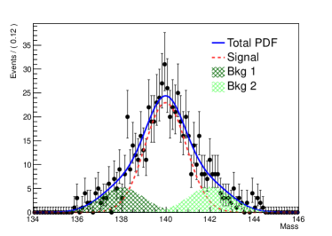
Figure 1: Example toy experiment drawn from Eq. V, with $N_{s,t}=500$ and $N_{b1,t}=N_{b2,t}=100$.

In Figure 2 we show the pull distributions of each pull definition in Section IV, using 5000 toy experiments. While the standard definition Eq. 9 is consistent with a unit Gaussian ($\mu_{p}=-0.031\pm 0.014$, $w_{p}=0.993\pm 0.011$), the other definitions (12, 13) are not. When enlarging the sample sizes to $N_{t}=70\,000$, the distributions remain unchanged.

In Figure 3 we show again the three pull distributions for generating and fitting the “wrong way”. Now definitions Eq. 12 and Eq. 13 follow a unit Gaussian, while definition Eq. 9 does not. However, this depends on the width of the constraint. These examples support our conclusion of Section IV.

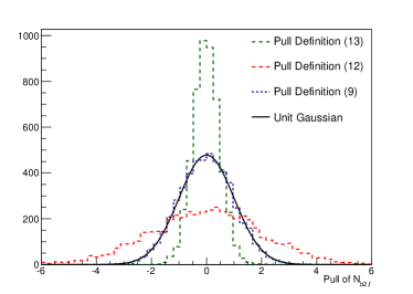
Figure 2: Pull distributions according to Eq. 9 (blue), Eq. 12 (red), and Eq. 13 (green). Overlaid is a unit Gaussian (dashed).

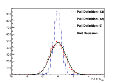
Figure 3: Distributions of the same pull definitions as described in the caption of Figure 2, but when performing toy experiments in the “wrong way”.

To illustrate how a tight constraint term can push the fit into the type A EML regime, we now subsequently tighten the constraints on the $N_{bi}$ we observe in Figure 4 that the difference between fitted and generated total number of events $N_{f}-N^{\prime}$ can grow larger, as the constraints get stronger. The widest distribution is reached at a value of about $\sqrt{N_{bi,t}}$. Then, deviations of up to $\approx 10$ events are possible, corresponding to $\approx 1.4\%$ of the events in the considered scenario.

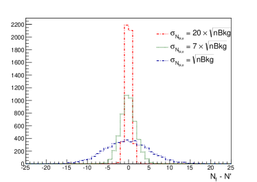
Figure 4: Distribution of the difference of fitted and generated total number of events $N_{f}-N^{\prime}$ for different values of the constraint width on the $N_{bi}$: $\sigma_{N_{bi,e}}=200$ (red), $70$ (green), $10$ (blue).

VI RooFit

The RooFit framework roofit is widely used in experimental particle physics to implement sophisticated maximum likelihood fits. It also features a mechanism to automate pull studies, RooMCStudy. We would like to point out several pitfalls present in RooFit version $3.5.4$ (bundled with Root version $5.34.00$).

There are two ways to configure RooMCStudy for the use with constraint terms. The first, using the Constrain() argument, is supposed to be used when the constraint term is part of the original PDF definition. The second, using the ExternalConstraints() argument, should be used when the constraint terms are supplied separately. Both ways do not give identical results. In the following, we refer to pulls obtained through RooMCstudy::plotPull().

Using Constrain(): RooMCstudy generates the “wrong way” sketched in Section III. This is particularly important if constraints on yield parameters are present. Then, RooFit first fluctuates the expected yield using the constraint term, and then again fluctuates the result using the EML Poisson term. As a consequence, the total generated yield does not follow a Poissonian anymore. For the pull computation Eq. 13 is used. If the width of a yield constraint is much larger than $\sqrt{N}$, one expects results similar to those obtained in the unconstrained situation. But in our example scenario, we observe a moderate bias of $\mu_{p}=0.3$. Also, the distributions of both the central value and the error are much wider compared to the unconstrained situation. This is shown in Figure 5. It can also happen, that the effects cancel by chance: In a second test scenario, corresponding to Eq. 1, with $N_{s,t}=1000$, $N_{b,t}=500$, and $G(N_{b};\mu=N_{b,t},\sigma=150)$, we observed a unit Gaussian pull, while the error and central value distributions of $N_{b}$ were still too wide.

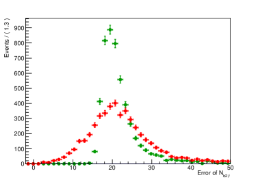
Figure 5: Error distribution (red) obtained from RooMCstudy when using the Constrain() approach and a wide constraint $G(N_{bi};\mu=N_{bi,t},\sigma=N_{bi,t})$. Also shown is the error distribution in the unconstrained case (green).

Another pitfall when using Constrain() is that if the generateAndFit() function is called in an EML scenario, and if one explicitly specifies the total number of events to be generated in the function call, then the pulls depend on the width of the constraint: For wide constraints, the pull distribution will be too wide. This is illustrated in Figure 6.

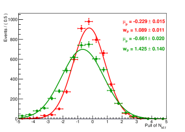
Figure 6: Pull distribution (red) obtained from RooMCstudy when using the Constrain() approach and a wide constraint $G(N_{bi};\mu=N_{bi,t}=100,\sigma=N_{bi,t})$. The other distribution (green) is for the same scenario, but obtained by explicitly stating $N_{t}=700$ in the generateAndFit() function call.

Using ExternalConstraints(): RooMCstudy generates the “right way”, i.e. the component yields fluctuate like a Poissonian. But during fitting, always the same, fixed constraint is used, and the pull is computed using Eq. 9. As a consequence, the resulting pull distribution is too narrow. Thus, if the constraint is wide enough compared to $\sqrt{N}$, the unconstrained situation is recovered. This is illustrated in Figure 7.

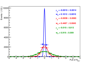
Figure 7: Pull distribution obtained from RooMCstudy when using the ExternalConstraints() approach and a wide constraint $G(N_{bi};\mu=N_{bi,t}=100,\sigma=50)$ (green), a medium constraint ($\sigma=10$, red), and a narrow constraint ($\sigma=1$, blue).

Considering these difficulties it is clear that, in order to be able to conclude on a potential fit bias, the user needs a detailed understanding of RooMCstudy.

VII Conclusion

We have discussed the basic features of extended maximum likelihood fits, and how to use constraint terms to incorporate external knowledge into these fits. If constraint terms are present, the generation of pseudo datasets requires care. We recommend to use the “right way”, in which the constraint is fluctuated in the generation step and the PDF is not, and to use the usual pull definition. Then we find the pull to follow a unit Gaussian even if constraints on yield parameters are present.

The authors wish to thank Niels Tuning for useful discussion.

References

- (1) R. J. Barlow, Nucl.Instrum.Meth. A297, 496 (1990).
- (2) CDF Statistics Commitee, L. Demortier and L. Lyons, CDF Public Note 5776 (2002).
- (3) W. Verkerke and D. Kirkby, http://roofit.sourceforge.net.