Stability and robustness analysis of cooperation cycles driven by destructive agents in finite populations

Abstract

The emergence and promotion of cooperation is one of the main issues in evolutionary game theory, as cooperation is amenable to exploitation by defectors, which take advantage from cooperative individuals at no cost dooming them to extinction. It has been recently shown that the existence of purely destructive agents (termed jokers) acting on the common enterprises (public goods games), can induce stable limit cycles between cooperation, defection and destruction when infinite populations are considered. These cycles allow for time lapses in which cooperators represent a relevant fraction of the population, providing a mechanism for the emergence of cooperative states in nature and human societies. Here we study analytically and through agent-based simulations the dynamics generated by jokers in finite populations for several selection rules. Cycles appear in all cases studied thus showing that the joker dynamics generically yields a robust cyclic behavior not restricted to infinite populations. We have also computed the average time in which the population consists mostly of just one strategy and compare the results with numerical simulations.

I Introduction

Cooperation is necessary for the appearance of complex structures and higher order selection units from individual behaviors. In this way, cooperation between unicellular life forms gave rise to multicellular organisms, cooperative animals form communities and cooperation between humans gives rise to the complex societies we live in (maynard-smith:1995, ). Thus, it is very important to understand the conditions that allow cooperation to thrive and evolve in nature and society. However, cooperative behaviors are not stable, as they are easily invaded by selfish individuals, who benefit from the interactions with cooperative ones but avoid paying the costs attached to cooperation. The selfish individuals, called defectors, have a higher fitness —a measure of reproductive success— than cooperators in any well mixed population, and therefore will spread under the action of natural selection, leading to the extinction of the cooperative behavior (hofbauer:1998, ), and to populations where nobody benefits from altruistic acts (the “tragedy of the commons” (hardin:1968, )).

In the last decades the study of the Public Goods (PG) game, a mathematical metaphor of a common enterprise, in which cooperative individuals invest —pay a cost— and share the benefits with all the players involved in the game, has led to the discovery of some mechanisms that allow cooperation to thrive, as introducing reputation (milinski:2005, ), diversity in number and size of groups (santos:2008, ), linking group size and payoffs (wakano:2009, ), or the inclusion of spatial structure and conditional behaviors (roca:2009c, ; szolnoki:2011, ; szolnoki:2012, ). Furthermore, it has been proven that the introduction of some behavioral types in well-mixed population, as punishers (fehr:2002, ; hauert:2007, ) or individuals which do not participate in the PG and instead receive a fixed benefit (the so-called ‘loners’) (hauert:2002b, ), may promote cooperation. However, the only behavioral type found so far that allows for the emergence of stable cycles in the presence of mutations is the so called joker strategy (arenas:2011, ). Jokers do not take part of the benefits produced by the PG game and instead they provoke a damage to the common enterprise, thus affecting every individual involved in it. Surprisingly, the effect of these indiscriminate destructive agents on the dynamics is the induction of robust evolutionary stable limit cycles of cooperation, defection and destruction. A cyclic dynamics can also be found when loners are involved. However, jokers induce cycles that are dynamically different from those found with loners (hauert:2002b, ), because the latter are neutrally stable (i.e, have no fixed amplitudes) and disappear in the presence of mutations or structural noise.

The inclusion of destructive agents in the PG game is motivated by the observation that, in nature and society, the appearance of a risk, as those created by common enemies, predators or simply dangerous situations, may induce cooperation among the victims (lavalli:2009, ; krams:2010, ).

In a previous work (arenas:2011, ), the stability of the evolutionary cycles induced by jokers was proven for infinite populations through the analysis of the replicator mutator equation. Here, we extend the study to finite populations and analyze the dynamics for different updating methods (szabo:2007, ), i.e., different selection dynamics for the population, in order to analyze if robust cycles are also found. The conclusion we reach from this study is that the robust cycles obtained using the replicator-mutator equation are not just restricted to this particular dynamics but are a generic feature of the joker model.

The paper is organized as follows. In section II we explain the PG game and review the dynamics in infinite populations. Section III provides the stochastic equations describing the evolutionary dynamics for finite populations. In section IV we analyze the joker dynamics in finite populations using different selection dynamics in order to check the existence of cycles. Section V is devoted to conclusions.

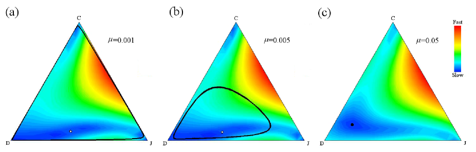
Figure 1: (Color online.) Cycles induced by jokers in infinite populations. The simplexes describe the replicator-mutator dynamics for a population of cooperators, defectors and jokers with parameter values satisfying $n>r>1+d(n-1)$, for which a rock-paper-scissor dynamics is expected. For small mutation rates, the only equilibrium is a repeller (white dot in (a),(b)), and trajectories end up in a stable limit cycle of decreasing amplitude with increasing $\mu$ (black line); when mutations reach a critical value $\mu_{c}$, the system undergoes a Hopf bifurcation and a stable mixed equilibrium appears (black dot in (c)). Thus the presence of jokers induces periodic bursts of cooperation for low mutation rates, and stable coexistence for high $\mu$. Parameters: $n=5$, $r=3$, $d=0.4$, $\mu$ is (a) 0.001, (b) 0.005, (c) 0.05. (Images generated using a modified version of the Dynamo Package (sandholm:2007, )).

II Evolutionary cycles induced by jokers in Public Good games

In each PG game a number $n$ of individuals is randomly chosen from the entire population. Each cooperative individual contributes to the common enterprise at a cost $c$ to itself, which yields a benefit $b=rc$ ($r>1$) equally distributed between all players; defectors free-ride the public good at no cost, thus obtaining a higher benefit than cooperators; jokers do not participate on the benefits, and each one provokes a damage $-d<0$ to be shared by all individuals engaged in the PG game. Note that the cost paid by C players can be set to $c=1$ without loss of generality: all other payoffs are given in units of $c$.

Let us call $0\leq m\leq n$ the number of cooperative participants, $0\leq j\leq n$ the number of jokers, $n-m-j\geq 0$ the number of defectors and $S=n-j$ the number of non-jokers, i.e., the number of individuals involved in the PG game, and that potentially benefit from the PG. Then the payoff of a defector will be $\Pi_{\rm D}(m,j)=(rm-dj)/S$, and that of a cooperator $\Pi_{\rm C}=\Pi_{\rm D}-1$; as previously stated, in each interacting group defectors will always do better than cooperators. Jokers’ payoff is always $0$.

In summary, we have

$$\Pi_{\rm D}(m,j)=\frac{rm-dj}{S}, 0\leq m\leq S-1\leq n-1,$$

$$\Pi_{\rm C}(m,j)=\frac{rm-dj}{S}-1, 1\leq m\leq S\leq n,$$ (1)

$$\Pi_{\rm J}(m,j)=0, 0\leq S\leq n-1.$$

A simple invasion analysis arenas:2011 shows that the PG thus defined determines a tragedy of the commons hardin:1968 for $r<r_{\rm max}=n(M-1)/(M-n)$, where $M$ is the population size. For infinite populations, the latter condition reduces to $r<n$, as usual in PG games. Therefore, a mixed population of cooperators and defectors with $r<r_{\rm max}$ will end up composed of defectors only. The interesting question is then if jokers may prevent the extinction of cooperators and under which conditions. In Ref. arenas:2011 , it was shown that, in the region of interest, namely $1<r<r_{\rm max}$, $d>0$, the system exhibits: (a) joker-cooperator bistability for $1+d/(M-1)<r<1+(n-1)d$, (b) joker dominance for $r<1+d/(M-1)$ and, most importantly, (c) a rock-paper-scissor (RPS) cyclic dominance of the three strategies for

$$r>1+(n-1)d.$$ (2)

This condition expresses the fact that a single cooperator gets a positive payoff in spite of the damage inflicted by $n-1$ jokers, which allows cooperators to thrive in the damaging environment that represents a population of jokers and re-establish a cooperative environment. In Ref. arenas:2011 , we analyzed just one dynamics, namely the replicator-mutation dynamics, and showed that it produces stable (robust) limit cycles C$\to$D$\to$J$\to$C when mutations are rare, and stable coexistence for high mutation rates (Fig. 1). In the following we will analyze the dynamics of PG with jokers in finite populations under different update rules, check the appearance of cycles and calculate the average time spent in each homogeneous state, in order to decide which dynamics better promotes the survival of cooperation.

III Stochastic dynamics in finite populations

The deterministic evolution represented by the replicator-mutator equation is an idealization of the system behavior in the limit of infinite populations. To get a deeper insight into the model we need to address the question what happens when populations have a finite size $M$. To begin with we need to describe the microscopic dynamics in more detail. Hauert et al. hauert:2007 have proposed a protocol in which random selections of $n$ players are gathered together to play the game. After receiving their corresponding payoffs the group dissolves and a new one is sampled. This sampling is made a sufficient number of times so that on average each player receives a payoff proportional to the mean payoff she can obtain given the composition of the population.

Suppose there are $m$ cooperators, $j$ jokers, and $M-m-j$ defectors in the population. The probability that the sampling of $n$ individuals contains $k$ cooperators, $l$ jokers, and $n-k-l$ defectors is given by the extended hypergeometric distribution

$$p(k,l|n,m,j,M)=\frac{\displaystyle\binom{m}{k}\binom{j}{l}\binom{M-m-j}{n-k-l}}{\displaystyle\binom{M}{n}}.$$ (3)

The average payoff of strategy X within this population, $P_{\rm X}(m,j)$, is obtained by averaging formulae (1) with this probability distribution. This is done in Appendix A, where explicit expressions for $P_{\rm C}(m,j)$ and $P_{\rm D}(m,j)$ are obtained —obviously $P_{\rm J}(m,j)=0$ irrespective of the population composition.

Once payoffs are obtained evolution proceeds by imitation. Different payoff-dependent updating rules have been proposed in the literature szabo:2007 . All of them describe a process of birth and death which is defined by the transition probability $T(m^{\prime},j^{\prime}|m,j)$ from a population with composition $(m,j)$ to another one with composition $(m^{\prime},j^{\prime})$ within the set

$$\begin{split}\mathcal{N}_{m,j}=&\,\{(m,j),(m\pm 1,j),(m,j\pm 1),\\ &(m+1,j-1),(m-1,j+1)\}.\end{split}$$ (4)

If now $\Pi(m,j;t)$ denotes the probability that the population has a composition given by $(m,j)$ at time $t$, then this probability evolves according to

$$\Pi(m,j;t+1)=\sum_{(m^{\prime},j^{\prime})\in\mathcal{N}_{m,j}}T(m,j|m^{\prime},j^{\prime})\Pi(m^{\prime},j^{\prime};t).$$ (5)

It is implicitly asumed that $\Pi(m,j;t)=0$ for all $t$ if the pair $(m,j)$ is outside the set $\mathcal{P}\equiv\{(m,j)\in\mathbb{Z}^{2}:m,j\geq 0$, $m+j\leq M\}$.

If we introduce matrix $\mathbf{T}$, with elements $T(m,j;m^{\prime},j^{\prime})$ [$(m,j)$ is the “row index” and $(m^{\prime},j^{\prime})$ the “column index”] defined as

$$T(m,j;m^{\prime},j^{\prime})=\begin{cases}T(m,j|m^{\prime},j^{\prime})&\text{if $(m^{\prime},j^{\prime})\in\mathcal{N}_{m,j}$,}\\ 0&\text{otherwise,}\end{cases}$$ (6)

and vectors $\boldsymbol{\Pi}(t)$, with elements $\Pi(m,j;t)$ [where $(m,j),(m^{\prime},j^{\prime})\in\mathcal{P}$], then Eq. (5) can be cast in matrix notation simply as

$$\boldsymbol{\Pi}(t+1)=\mathbf{T}\,\boldsymbol{\Pi}(t).$$ (7)

III.1 Stationary state

If the process undergoes mutations then matrix $\mathbf{T}$ is ergodic and Eq. (7) has got a unique stationary state, $\boldsymbol{\pi}$, which is obtained by solving the linear system

$$\boldsymbol{\pi}=\mathbf{T}\boldsymbol{\pi}.$$ (8)

In the absence of mutations, though, there are three absorbing states corresponding to the three homogeneous populations. A homogeneous population remains invariant because the imitation process cannot change its composition. We will denote these vectors $\mathbf{e}_{\rm C}$, $\mathbf{e}_{\rm D}$, $\mathbf{e}_{\rm J}$, the index denoting the strategy of the homogeneous population. Clearly $e_{\rm C}(m,j)=\delta_{m,M}\delta_{j,0}$, $e_{\rm D}(m,j)=\delta_{m,0}\delta_{j,0}$, $e_{\rm J}(m,j)=\delta_{m,0}\delta_{j,M}$.

III.2 Infinitely small mutation rate

After every imitation attempt (whether successful or not), individuals can randomly mutate their strategy. With probability $2\mu$ the actor of the imitation event changes its current strategy into one of the other two equally likely. Parameter $\mu$ is referred to as the mutation ratio. In this section we will be concerned with mutation rates $\mu\ll 1$.

In the the limit $\mu\to 0^{+}$ the stationary probability distribution must be a linear combination of the stationary vectors of the process without mutations, so in principle, taking the limit

$$\lim_{\mu\to 0^{+}}\boldsymbol{\pi}=\sum_{{\rm X}={\rm C},{\rm D},{\rm J}}\alpha_{\rm X}\,\mathbf{e}_{\rm X}$$ (9)

should provide the coefficients $\alpha_{\rm X}$ of this linear combination, but this limit cannot be obtained directly from Eq. (8). There is an alternative though. It has been proven fudenberg:2006 that the $\mu\to 0^{+}$ limit of this process is equivalent to another process with three states, C, D, J, in which the transition probability between X and Y is equal to the probability that a single mutant of type Y invades an otherwise homogeneous population of X individuals, thus transforming it into a homogeneous population of Y individuals. Intuitively, this is tantamount to saying that mutations are so rare that the ultimate fate of a mutant is decided before the next mutation occurs. The stationary vector in this space,

$$\boldsymbol{\alpha}=(\alpha_{\rm C},\alpha_{\rm D},\alpha_{\rm J}),$$ (10)

provides the values of the coefficients $\alpha_{\rm X}$ in (9).

Following hauert:2007 , let $\rho_{\rm YX}$ denote the probability that a single Y mutant takes over the population made of the mutant and $M-1$ individuals of type X. Then the transition probability of going from state X to a different state Y in the three-states Markov chain defined above will be $r_{\rm YX}=\rho_{\rm YX}\mu$. Introducing $\mathbf{R}=(r_{\rm YX})$ so that the elements in each column add up to one (this fixes the diagonal of the matrix), we can rewrite this matrix as $\mathbf{R}=\mathbf{I}+\mu\mathbf{Q}$, where

$$\mathbf{Q}=\begin{pmatrix}-\rho_{\rm DC}-\rho_{\rm JC}&\rho_{\rm CD}&\rho_{\rm CJ}\\ \rho_{\rm DC}&-\rho_{\rm CD}-\rho_{\rm JD}&\rho_{\rm DJ}\\ \rho_{\rm JC}&\rho_{\rm JD}&-\rho_{\rm CJ}-\rho_{\rm DJ}\end{pmatrix}.$$ (11)

Vector $\boldsymbol{\alpha}$ is then the solution of the linear system $\mathbf{Q}\boldsymbol{\alpha}=\mathbf{0}$. A little bit of algebra leads to the result

$$\alpha_{\rm C} =(\rho_{\rm CD}\rho_{\rm CJ}+\rho_{\rm CD}\rho_{\rm DJ}+\rho_{\rm CJ}\rho_{\rm JD})/A,$$ (12)

$$\alpha_{\rm D} =(\rho_{\rm DC}\rho_{\rm DJ}+\rho_{\rm DC}\rho_{\rm CJ}+\rho_{\rm DJ}\rho_{\rm JC})/A,$$ (13)

$$\alpha_{\rm J} =(\rho_{\rm JC}\rho_{\rm JD}+\rho_{\rm JC}\rho_{\rm CD}+\rho_{\rm JD}\rho_{\rm DC})/A,$$ (14)

with $A$ chosen so as to fulfill

$$\sum_{{\rm X}={\rm C},{\rm D},{\rm J}}\alpha_{\rm X}=1.$$ (15)

III.3 Finite mutation rates

If the mutation rate is not zero the Markov chain is ergodic and the stationary state can be obtained by solving numerically Eq. (8). This is accomplished with better accuracy by splitting

$$\mathbf{T} =\mathbf{T}_{0}+\mathbf{T}_{1},$$ (16)

$$\boldsymbol{\pi} =\sum_{{\rm X}={\rm C},{\rm D},{\rm J}}\alpha_{\rm X}\,\mathbf{e}_{\rm X}+\boldsymbol{\pi}_{1},$$ (17)

with $\mathbf{T}_{0}$ the transition matrix in the absence of mutations—i.e., with transitions describing only the imitation process. Then $\boldsymbol{\pi}_{1}$ is the solution of the linear system

$$(\mathbf{I}-\mathbf{T})\boldsymbol{\pi}_{1}=\sum_{{\rm X}={\rm C},{\rm D},{\rm J}}\alpha_{\rm X}\,\mathbf{T}_{1}\mathbf{e}_{\rm X}.$$ (18)

III.4 Imitation rules

In order to specify the transition matrix $\mathbf{T}$ we need to describe the imitation process. Of the many different rules applied in the literature szabo:2007 we have chosen the three most commonly employed: unconditional imitation, proportional update, and a Moran process. In all cases the corresponding matrix $\mathbf{T}$ is obtained in Appendix B.

Under unconditional imitation two players are chosen at random among the population, one as the focal player and the other one as the model to imitate. The focal player compares both payoffs and changes her strategy to that of the model if the latter has a higher payoff. In this case, the strategy with the highest fitness never changes except by mutation, which is the only source of stochasticity in this rule.

Appendix C discusses the value $\boldsymbol{\alpha}$ for this update rule. There are two possibilities:

1. $r>1+(n-1)d$. In this cases all three homogeneous states are equally likely [c.f. Eq. (41)].

2. $r<1+(n-1)d$. In this cases J is the only absorbing state of the process [c.f. Eq. (43)].

Proportional update is entirely similar to unconditional imitation with the exception that imitation occurs with probability proportional to the payoff difference between the model and the focal players. For this reason the values of $\boldsymbol{\alpha}$ for this rule are the same as those for unconditional imitation.

In a Moran process a strategy is chosen to be imitated (or reproduced) with a probability proportional to its population-dependent fitness. The player who imitates (or is replaced by the offspring of) this selected player is randomly chosen from the rest of the population. The only drawback of this rule is that fitnesses must be positive for it to make sense, so they cannot be directly the payoffs of the game, because they can take negative values. A standard mapping between payoff and fitness is obtained by introducing the selection strength $s$ nowak:2004a . This weights the contribution of the game to the total fitness of the strategy as $F=1-s+sP$, with $P$ the average payoff. Bounding the value of $s$ we can force $F$ to be positive.

The Moran process thus described defines a birth-death process with two absorbing states, and the corresponding probabilities $\rho_{\rm XY}$ are obtained via standard formulae (see Appendix C).

IV Results: Robustness of the cycles using different selection dynamics

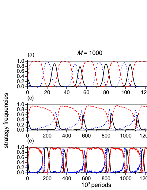
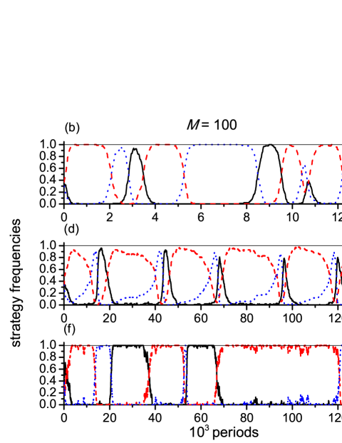
Figure 2: (Color online.) Time evolution of the frequencies of the three strategies in a population of $M=1000$ (left) and $M=100$ (right) individuals playing a PG with jokers with different update rules: (a), (b) unconditional imitation, (c), (d) proportional update, and (e), (f) a Moran process. The presence of jokers induces a cyclic behavior irrespective of the update rule and the population size, as long as the mutation rate $\mu>0$. Black solid lines: cooperators, red dashed lines: defectors, and blue dotted lines: jokers. One period corresponds to one updating event according to the evolutionary rule used. Parameters $n=5,r=3,d=0.4$, $\mu=0.001$; in (a)-(d) $s=1$, in (e),(f) $s=0.38$.

In this section we compare the results of agent-based simulations with those obtained by solving the stationary equation (8). Simulations implement the following stochastic process. We start with a population of $M$ individuals with equal amounts of C, D and J players. Then:

1. Assuming that every time step each individual plays many rounds of the game with different, randomly gathered groups of $n$ players, the payoffs they obtain will be proportional to the average payoffs, as calculated in Appendix A. Thus we assume that these expressions provide the payoffs each individual gains every time step.

2. These payoffs are used to update the population according to the corresponding imitation rule. We implement the three rules described in Sec. III.4.

3. With probability $\mu$ each newborn mutates to a different strategy (any of the other two with equal probability).

A quite general result is that, irrespective of the population size, at low mutation rates simulations show patterns of cyclic invasions C$\to$D$\to$J$\to$C (see Fig. 2). These patterns resemble the limit cycles observed in the replicator dynamics, i.e., for infinite populations arenas:2011 (c.f. Fig. 1).

Roughly speaking we can distinguish three regimes of mutations. In the low mutation regime the system spends most of the time in homogeneous states, and the dynamics of the system is well described by the $\mu\to 0$ limit of the stationary probability distribution $\boldsymbol{\pi}$. This can be clearly seen in Fig. 3. The dashed-dotted curves in Figs. 3(a), (c) and (e) represent the fraction of time spent in transients when a homogeneous population is replaced by another one arisen as the result of mutations. This fraction is very small for $\mu\lesssim 10^{-5}$–$10^{-4}$, depending on the imitation rule. For larger mutation rates ($10^{-5}$–$10^{-4}\lesssim\mu\lesssim 10^{-3}$–$10^{-2}$) the system spends as much time in homogeneous populations as in mixed transient states. This is the regime displayed in Fig. 2, where cycles are clearly defined even though for some imitation rules (particularly so for proportional update) certain homogeneous populations that are hardly ever reached [Fig. 2(b) shows burst of cooperators which never reach a fraction higher than 80% of the population]. For even higher mutation rates homogeneous populations are very rare and the behavior of the system is very different, typically dominated by defectors [see Figs.3(b), (d) and (f)].

(a)	(b)
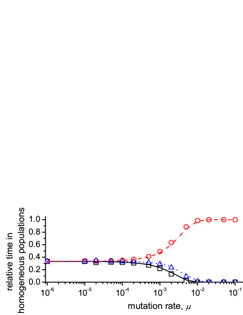
(c)	(d)
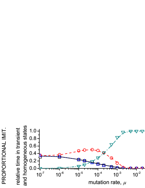
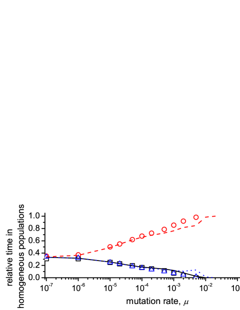
(e)	(f)

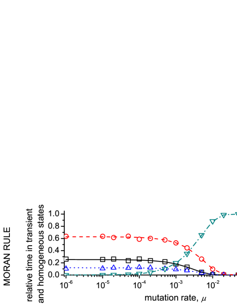
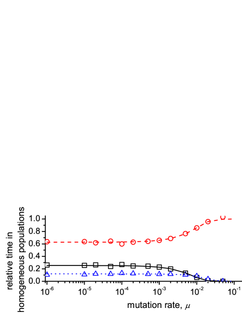
Figure 3: (Color online.) Relative times spent in homogeneous as well as in transient states in a population of $M=100$ individuals. For practical purposes, a state is considered homogeneous if more than 95% of individuals belong to the same strategy. Symbols are the result of agent-based simulations; lines are obtained from the solution of Eqs. (17)–(18). Results for cooperators are represented with (black) squares and solid lines, those for defectors with (red) circles and dashed lines, and those for jokers with (blue) triangles and dotted lines. Panels (a), (c) and (e) also show (with inverted triangles and dashed-dotted lines) the fraction of time spent in transient states. Panels (b), (d) and (f) show the fractions of the time spent in each of the three homogeneous states relative to the total time spent in homogeneous states. Panels (a) and (b) correspond to unconditional imitation, panels (c) and (d) to proportional update, and panels (e) and (f) to a Moran rule. We can see that high mutation rates promote defection over the other two strategies. Parameters used are $n=5,r=3,d=0.4$; selection strength is $s=1$ in (a)–(d) and $s=0.38$ in (e) and (f).

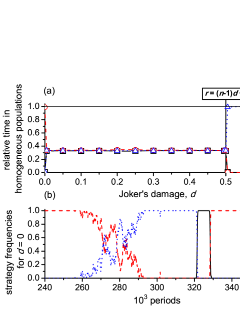
Figure 4: (Color online.) Evolution of a population of $M=100$ individuals by unconditional imitation. (a) Fraction of time spent in homogeneous populations of cooperators (black squares and solid line), defectors (red circles and dashed line) and jokers (blue triangles and dotted line), as a function of joker’s inflicted damage $d$. Symbols correspond to an agent-based simulation; lines to the results obtained from numerical computation of the stationary probability distribution. (b) A realization made with $d=0$ showing an invasion of defectors by jokers through pure drift, and the subsequent burst of cooperators and turn-over by defectors. Parameters: $n=5,r=3,s=1$ and $\mu=5\times 10^{-5}$.

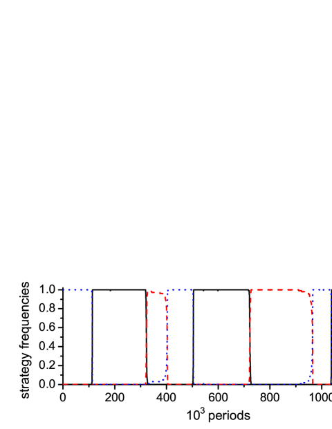
Figure 5: (Color online.) Realization of an agent-based simulation of a population with $M=100$ individuals evolving through proportional update. Notation is as in Fig. 4. Parameters: $n=5,r=3,d=0.4,\mu=5\times 10^{-6},s=1$.

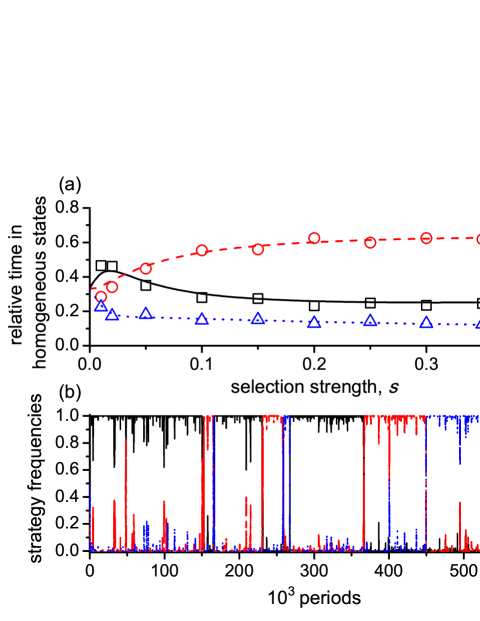
Figure 6: (Color online.) A population of $M=100$ individuals evolving through Moran update. (a) Comparison of the the relative times in which the population is in a homogeneous state vs. the selection strength, $s$, for low mutation rates. Lines represent the analytical estimates obtained in Sec. C.2; symbols represent the results from agent-based simulations. (b) Fractions of each strategy as a function of time as obtained from a realization of an agent-based simulation. Cooperators are represented with a black solid line and squares, defectors with a red dashed line and circles, and jokers with a blue dotted line and triangles. Parameters are $n=5,r=3,d=0.4$ and $\mu=5\times 10^{-5}$. In (b) the selection strength is $s=0.05$.

Unconditional imitation is practically a deterministic rule in the low mutations regime. For $\mu\lesssim 10^{-4}$ the population is almost always homogeneous, and is made of each of the three strategies with equal probability [see Figs. 2(a), (b) and Figs. 5(a), (b)]. Figure 3(a) shows this probability as a function of the joker’s inflicted damage $d$. As long as $d>0$ and $r>1+(n-1)d$ we find each strategy equally likely. For $r<1+(n-1)d$ a homogeneous population of jokers cannot be invaded because this is the only absorbing state of the Markov chain for $\mu=0$. For $d=0$ jokers do not inflict damage. Then the system spends most of the time in a homogeneous population of defectors. However, random drift allows for occasional invasions by jokers, who are subsequently wiped out by cooperators, who in its turn get replaced again by defectors. Figure 4(b) illustrates a typical realization exhibiting one of these turn-overs.

As of proportional update, its main difference with unconditional imitation is its being a truly probabilistic rule, in which individuals only imitate higher payoffs with a certain probability. Although in the small mutations regime this leads to the same probability of mutual invasion of strategies as for unconditional imitation, the stochastic nature of this rule renders much longer invasion times. This can be clearly appreciated in Fig. 2.

Another effect of stochasticity is that the time spent in transient states is also longer, thus shrinking the low mutations regime by more than one order of magnitude [compare Figs. 3(a) and (c)]. The effect is particularly notorious for jokers, who take a long time to invade defectors, thus extending the life time of defective populations. This effect is illustrated in Fig. 5, which represents a typical realization of an agent-based simulation.

The Moran process is the randomest of the three evolutionary dynamics because even strategies not performing very well have a chance to get imitated. The effect is more noticeable the smaller the population. This dynamics imposes an upper limit to the selection strength $s$ (see Sec. III.4) and the probabilities to find the population in each of the three homogeneous states depend on the parameters of the game and on $s$ in a nontrivial way (see Sec. C.2). These probabilities are represented in Fig. 6(a) as a function of $s$. The theoretical predictions of Sec. C.2 agree with the simulations. This figure shows that cooperation is highly promoted for small $s$($0.005<s<0.05$). In this limit cooperative populations are found with almost 50% probability. This probability decreases down to around 25% for larger $s$. Figure 6(b) shows a typical realization of this process, exhibiting a defining feature of this process, namely the frequent failures of attempted invasions.

(a)	(b)	(c)
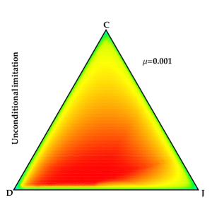
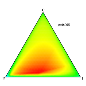
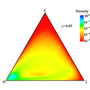
(d)	(e)	(f)
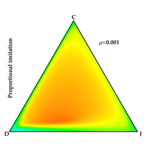
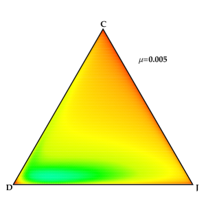
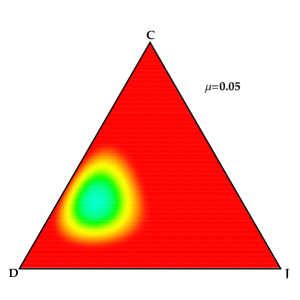
(g)	(h)	(i)

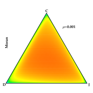
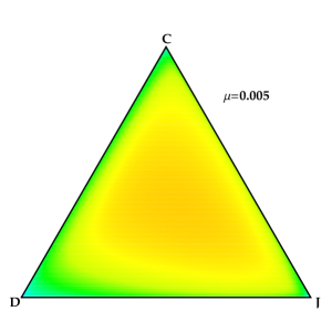
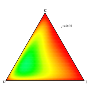
Figure 7: (Color online.) Density plots for the probability of finding the system in each population state as obtained by solving numerically Eq. (8). First row corresponds to unconditional imitation, second row to proportional imitation, third row to a Moran process. In each case mutations increase left to right. In all three cases low mutation rates ($\mu$) yield high probabilities near the boundaries of the simplexes, specially near the corners, corresponding to cyclic transitions between homogeneous states. Increasing $\mu$ increases the probability to find the system near homogeneous defective populations. For high $\mu$ an attractive point appears close to the D corner which goes away from it upon increasing $\mu$. Parameters are $n=5,r=3,d=0.4$; the selection strength is $s=1$ in the first and second rows, $s=0.38$ in the third. Mutation rates have been chosen as in Fig. 1 and appear near each simplex. Densities are plotted using a logarithmic scale.

Whichever the update rule, when mutation rates are not small the system is better characterized by providing the stationary probability distribution $\pi$, as obtained from Eq. (18)). The results are plotted in Fig. 7 for all three imitation rules and different mutation rates $\mu$. For low and intermediate values of $\mu$ the higher probabilities are found near the border of the simplexes, consistent with the cyclic behavior of the system. However, for high $\mu$ the probability peaks around a point. This point is interior for the most stochastic rules, but corresponds to a defective population for unconditional imitation. The simplexes are obtained for the same parameter values as used in Fig. 1, so a direct comparison with the results of the replicator dynamics can be made.

V Discussion and conclusions

In this paper we have proven that the existence of jokers, i.e., individuals whose purely destructive behavior is directed against the common enterprises represented by PG games, allows for the emergence of robust evolutionary cycles in finite populations regardless of the updating method chosen. Together with a previous report arenas:2011 on the existence of limit cycles for infinite populations evolving via a replicator-mutator dynamics, our present results show that limit cycles are a generic feature of the dynamics generated by destructive agents, not restricted to a particular selection dynamics. In fact, this is a dynamical feature that makes this model different from other three-player games like that of loners (hauert:2002b, ), for which cycles are structurally unstable and their existence strongly depends on the absence of mutations and other kinds of perturbations.

In a recent paper (mobilia:2010, ) Mobilia has shown that, of the three possible outcomes of the replicator equation for rock-paper-scissors games hofbauer:1998 , namely (a) orbits are attracted towards an asymptotically stable mixed equilibrium, (b) orbits cycle around a neutrally stable mixed equilibrium, and (c) orbits go away from an unstable mixed equilibrium and approach the heteroclinic orbit defined by the border of the simplex (the case of the Joker game), adding mutations between the three strategies merges cases (a) and (b), both of which yielding a mixed equilibrium. Oscillations disappear in these two cases. The Loners game belongs to class (b). In contrast, the Joker case analysed in this paper belongs to class (c), with mutations generating an attractive, stable limit cycle. In this case the dynamics oscillates between the three strategies with well-defined and robust oscillations. We are not aware of any other game for which the inclusion of a simple behavioral type (jokers do not need memory, have no especial recognition abilities, and do not rely on any reputation generated along the game) leads to cycles which are robust to perturbations and have a well defined period and amplitude irrespective of the initial fractions of players.

We have expanded here these results and have proven that the oscillatory dynamics does not occur only for infinite (or very large) populations evolving under a replicator dynamics, but also in the case of finite populations and for different update rules. We have analyzed unconditional imitation, proportional update, and a Moran process. In all cases the system exhibits finite time lapses in which most of the population is composed by cooperative individuals, finding that the Moran process for low (but not extremely low) selection pressures is the most favorable to cooperation—as the system spends 50% of the time in cooperative states. Under unconditional imitation the system spends one third of the time in cooperative states, whereas the more stochastic nature of proportional update favors defection due to the slower invasion of jokers, and thus the system stays longer in defective states—especially so for high mutation rates.

Let us note that, if the damage $d$ inflicted by jokers is zero, jokers are not able to overcome defectors and oscillations are supressed. The system ends up in a steady population where cooperation becomes extinguished, both with and without mutations (arenas:2011, ). Indeed, this case is identical to the loner model when the benefit obtained by loners is also zero, situation in which both jokers and loners become simply non-participants in the game with the only effect of reducing the effective number of players (hauert:2002b, ; arenas:2011, ). We have shown here that for finite populations and $d=0$ random drift allows for bursts in which the system spends some time in fully cooperative states, but that the happening probability of such events is very low.

The existence of damaging agents, which are able to destroy the defective populations and lead to a state without cooperators and defectors, gives cooperators the chance to re-build cooperative enterprises, and thus promotes cooperation. This result, as well as modifications of the model presented here, might be interesting in the study of human evolution, where examples of destructive periods can be found along history as a result of revolutions or wars. It has been suggested that these destructive periods take place whenever a society reaches a point where the public goods fall below a certain threshold (turchin:2006, ). The Joker game shares this feature. Modifications of the model presented here may thus help explain not only how cooperation in animals arises whenever there is a risk or they face a predator, but also provide insights into the evolutionary cycles observed in human society.

Appendix A Average payoffs in a finite population

Let us denote $P_{\rm X}(m,l)$ the average payoff that a player of type X receives when the population is made of $m$ cooperators, $j$ jokers, and $M-m-j$ defectors. This average payoff is calculated by averaging the corresponding payoff (1) with the probability distribution (3). For defectors this implies

$$P_{\rm D}(m,j)=\sum_{\begin{subarray}{c}k,l\geq 0\\ k+l<n\end{subarray}}\frac{rk-dl}{n-l}p(k,l|n-1,m,j,M-1).$$ (19)

To perform this average it will prove convenient to factorize the probability distribution as the product of two standard hypergeometric distributions, i.e.,

$$p(k,l|n,m,j,M)=p(l|n,j,M)p(k|n-l,m,M-j).$$ (20)

where

$$p(l|n,j,M)=\frac{\displaystyle\binom{j}{l}\binom{M-j}{n-l}}{\displaystyle\binom{M}{n}}.$$ (21)

The first term in (20) is the probability of selecting $l$ jokers out of the population, and the second term is the conditional probability of subsequently selecting $k$ cooperators, given that we have already selected the $l$ jokers.

A useful identity of the hypergeometric distribution —consequence of the properties of the binomial coefficients— is

$$k\,p(k|n,m,M)=\frac{nm}{M}p(k-1|n-1,m-1,M-1).$$ (22)

Substituting factorization (20) into (19) and making use of this identity we readily obtain

$$\begin{split}P_{\rm D}(m,j)=&\,\frac{rm}{M-j-1}\sum_{l=0}^{n-1}\frac{n-l-1}{n-l}\,p(l|n-1,j,M-1)\\ &-d\sum_{l=0}^{n-1}\frac{l}{n-l}\,p(l|n-1,j,M-1).\end{split}$$ (23)

A new identity, namely

$$\frac{p(l|n-1,j,M-1)}{n-l}=\frac{M}{n(M-j)}p(l|n,j,M),$$ (24)

allows us to do the sum

$$\sum_{l=0}^{n-1}\frac{p(l|n-1,j,M-1)}{n-l}=\frac{M[1-p(n|n,j,M)]}{n(M-j)}.$$ (25)

It will prove convenient to introduce the function

$$\Xi(n,j,M)\equiv\frac{j}{M-j}\left[1-\frac{(j-1)\cdots(j-n+1)}{(M-1)\cdots(M-n+1)}\right],$$ (26)

in terms of which

$$\begin{split}1-p(n|n,j,M)&=1-\frac{j(j-1)\cdots(j-n+1)}{M(M-1)\cdots(M-n+1)}\\ &=\frac{M-j}{M}\left[1+\Xi(n,j,M)\right].\end{split}$$ (27)

This allows us to write

$$\sum_{l=0}^{n-1}\frac{p(l|n-1,j,M-1)}{n-l}=\frac{1+\Xi(n,j,M)}{n},$$ (28)

and using this in (23) obtain

$$P_{\rm D}(m,j)=\frac{rm[n-1-\Xi(n,j,M)]}{n(M-j-1)}-d\,\Xi(n,j,M).$$ (29)

As for the average payoff of a cooperator,

$$\begin{split}P_{\rm C}(m,j)&=-1+\sum_{\begin{subarray}{c}k,l\geq 0\\ k+l<n\end{subarray}}\frac{r(k+1)-dl}{n-l}\\ &\phantom{=}\times p(k,l|n-1,m-1,j,M-1)\\ &=r\sum_{l=0}^{n-1}\frac{p(l|n-1,j,M-1)}{n-l}-1+P_{\rm D}(m-1,j)\\ &=\frac{r}{n}[1+\Xi(n,j,M)]-1+P_{\rm D}(m-1,j).\end{split}$$ (30)

Therefore

$$\begin{split}P_{\rm C}(m,j)=&\,\frac{r}{n}\left(1+\frac{(n-1)(m-1)}{M-j-1}\right)-1\\ &+\left[\frac{r}{n}\left(1-\frac{m-1}{M-j-1}\right)-d\right]\Xi(n,j,M).\end{split}$$ (31)

Finally, $P_{\rm J}(n,j)=0$ because jokers get zero regardless of the composition of the population.

Appendix B Calculation of the transition matrices

Transition probabilities $T(m,j|m^{\prime},j^{\prime})$ are obtained according to the specified update rule. We will calculate those corresponding to the rules used in this work. But before we proceed let us introduce some shorthands. We will write $T_{\epsilon_{1},\epsilon_{2}}\equiv T(m,j|m+\epsilon_{1},j+\epsilon_{2})$, where $\epsilon_{1},\epsilon_{2}\in\{-1,0,1\}$. Also by $\omega^{\rm XY}_{\epsilon_{1},\epsilon_{2}}$ we will denote the probability that a player of type Y is chosen to be replaced by a player of type X when the population is made of $m+\epsilon_{1}$ cooperators, $j+\epsilon_{2}$ jokers, and $M-m-j-\epsilon_{1}-\epsilon_{2}$ defectors. Whether the Y player is finally replaced by an X one depends on mutations, thus

$$\begin{split}T_{1,0}=&\,\omega^{\rm DC}_{1,0}(1-2\mu)+\left(\omega^{\rm JC}_{1,0}+\omega^{\rm CC}_{1,0}\right)\mu,\\ T_{1,-1}=&\,\omega^{\rm JC}_{1,-1}(1-2\mu)+\left(\omega^{\rm DC}_{1,-1}+\omega^{\rm CC}_{1,-1}\right)\mu,\\ T_{-1,0}=&\,\omega^{\rm CD}_{-1,0}(1-2\mu)+\left(\omega^{\rm JD}_{-1,0}+\omega^{\rm DD}_{-1,0}\right)\mu,\\ T_{0,-1}=&\,\omega^{\rm JD}_{0,-1}(1-2\mu)+\left(\omega^{\rm CD}_{0,-1}+\omega^{\rm DD}_{0,-1}\right)\mu,\\ T_{-1,1}=&\,\omega^{\rm CJ}_{-1,1}(1-2\mu)+\left(\omega^{\rm DJ}_{-1,1}+\omega^{\rm JJ}_{-1,1}\right)\mu,\\ T_{0,1}=&\,\omega^{\rm DJ}_{0,1}(1-2\mu)+\left(\omega^{\rm CJ}_{0,1}+\omega^{\rm JJ}_{0,1}\right)\mu,\end{split}$$ (32)

In all cases there are two possibilities for a Y individual to become an X one, either a pair XY is selected, the update takes place and no mutation occurs, or another pair ZY is selected (with ${\rm Z}\neq{\rm X}$) but a mutation changes Z into X.

Finally, the probability that no change of strategy occurs $T_{0,0}=T(m,j|m,j)$ is obtained as

$$T_{0,0}=1-(1-\mu)\sum_{{\rm X}\neq{\rm Y}}\omega^{\rm XY}_{0,0}-2\mu\sum_{{\rm X}}\omega^{\rm XX}_{0,0},$$ (33)

where the subscript $0,0$ refers to a population made of $m$ cooperators, $j$ jokers, and $M-m-j$ defectors.

Notice that the expansion (17) readily follows from expressions (32) and (33).

B.1 Unconditional imitation

This rule prescribes that two players are selected at random from the population and the strategy of the model player (X) replaces that of the focal player (Y) if the latter has a lower payoff. Accordingly, if ${\rm X}\neq{\rm Y}$,

$$\omega^{\rm XY}_{\epsilon_{1},\epsilon_{2}}=\frac{n^{\rm X}_{\epsilon_{1},\epsilon_{2}}n^{\rm Y}_{\epsilon_{1},\epsilon_{2}}}{M(M-1)}\Theta\left(P^{\rm X}_{\epsilon_{1},\epsilon_{2}}-P^{\rm Y}_{\epsilon_{1},\epsilon_{2}}\right),$$ (34)

where $\Theta(x)=1$ if $x>0$ and $0$ otherwise, and $n^{\rm X}_{\epsilon_{1},\epsilon_{2}}$ denotes the number of individuals of type X in the population (e.g., $n^{\rm C}_{1,0}=m+1$, $n^{\rm D}_{1,0}=M-j-m-1$, $n^{\rm J}_{1,-1}=j-1$, $n^{\rm D}_{0,0}=M-j-m$, etc.). On the other hand, in order to account for mutations we must define

$$\omega^{\rm XX}_{\epsilon_{1},\epsilon_{2}}=\frac{n^{\rm X}_{\epsilon_{1},\epsilon_{2}}(n^{\rm X}_{\epsilon_{1},\epsilon_{2}}-1)}{M(M-1)}.$$ (35)

B.2 Proportional update

Similarly to the previous rule,

$$\omega^{\rm XY}_{\epsilon_{1},\epsilon_{2}}=\frac{n^{\rm X}_{\epsilon_{1},\epsilon_{2}}n^{\rm Y}_{\epsilon_{1},\epsilon_{2}}}{M(M-1)}\Psi\left(P^{\rm X}_{\epsilon_{1},\epsilon_{2}}-P^{\rm Y}_{\epsilon_{1},\epsilon_{2}}\right),$$ (36)

where $\Psi(x)=x/\Omega$ if $x>0$ and $0$ otherwise, $\Omega$ being a constant ensuring that $\Psi\left(P^{\rm X}_{\epsilon_{1},\epsilon_{2}}-P^{\rm Y}_{\epsilon_{1},\epsilon_{2}}\right)\leq 1$ (typically $\Omega$ is chosen as the largest possible payoff difference). As in the previous rule $\omega^{\rm XX}_{\epsilon_{1},\epsilon_{2}}$ is given by (35).

B.3 Moran process

In this case payoffs are replaced by fitnesses $F^{\rm X}_{\epsilon_{1},\epsilon_{2}}=1-s+sP^{\rm X}_{\epsilon_{1},\epsilon_{2}}$ (see Sec. III.4). Let us introduce the total fitness of the population

$$\Phi_{\epsilon_{1},\epsilon_{2}}\equiv\sum_{\rm X}n^{\rm X}_{\epsilon_{1},\epsilon_{2}}F^{\rm X}_{\epsilon_{1},\epsilon_{2}}.$$ (37)

The Moran rule specifies that a player is chosen for reproduction proportional to its fitness and the offspring replaces another randomly chosen individual from the rest of the population. So if ${\rm X}\neq{\rm Y}$,

$$\omega^{\rm XY}_{\epsilon_{1},\epsilon_{2}}=\frac{n^{\rm Y}_{\epsilon_{1},\epsilon_{2}}}{M-1}\,\frac{n^{\rm X}_{\epsilon_{1},\epsilon_{2}}F^{\rm X}_{\epsilon_{1},\epsilon_{2}}}{\Phi_{\epsilon_{1},\epsilon_{2}}},$$ (38)

and

$$\omega^{\rm XX}_{\epsilon_{1},\epsilon_{2}}=\frac{n^{\rm X}_{\epsilon_{1},\epsilon_{2}}-1}{M-1}\,\frac{n^{\rm X}_{\epsilon_{1},\epsilon_{2}}F^{\rm X}_{\epsilon_{1},\epsilon_{2}}}{\Phi_{\epsilon_{1},\epsilon_{2}}},$$ (39)

Appendix C Stationary probabilities in the weak mutation limit

C.1 Unconditional imitation and proportional update

According to the payoffs obtained in Appendix A:

1. $P_{D}(m,0)>P_{C}(m,0)$ for all $0<m<M$, so D always invades C, but C never invades D.

2. $P_{C}(m,M-m)>P_{J}(m,M-m)$ for all $0<m<M$, provided $r>1+(n-1)d$ (the rock-paper-scissors condition), so under this assumption C always invades J, but J never invades C.

3. $P_{J}(0,j)>P_{D}(0,j)$ for all $0<j<M$, so J always invades D, but D never invades J.

Therefore

$$\mathbf{Q}=\begin{pmatrix}-1&\phantom{-}0&\phantom{-}1\\ \phantom{-}1&-1&\phantom{-}0\\ \phantom{-}0&\phantom{-}1&-1\end{pmatrix}.$$ (40)

This implies

$$\alpha_{\rm C}=\alpha_{\rm D}=\alpha_{\rm J}=\frac{1}{3}.$$ (41)

On the other hand, if $r<1+(n-1)d$ neither C invades J nor vice-versa, so in this case

$$\mathbf{Q}=\begin{pmatrix}-1&\phantom{-}0&0\\ \phantom{-}1&-1&0\\ \phantom{-}0&\phantom{-}1&0\end{pmatrix},$$ (42)

which implies

$$\alpha_{\rm C}=\alpha_{\rm D}=0,\quad\alpha_{\rm J}=1.$$ (43)

C.2 Moran Process

The Moran process for a population with two strategies defines a birth-death process with two absorbing states. The details of the calculation of $\rho_{\rm YX}$ can be found in hauert:2007 and follow standard formulae for this kind of processes karlin:1975 . Summarizing, if we denote $P_{\rm YX}(m)$ the payoff received by a type Y individual when the population is made of $m$ Y individuals and $M-m$ X individuals, then

$$\rho_{\rm YX}^{-1}=\sum\limits_{m=0}^{M-1}q_{m},\qquad\rho_{\rm XY}=q_{M-1}\rho_{\rm YX},$$ (44)

where $q_{0}=1$ and

$$q_{m}=q_{m-1}\frac{1-s+sP_{\rm XY}(M-m)}{1-s+sP_{\rm YX}(m)},\qquad 0<m<M.$$ (45)

Payoffs $P_{\rm XY}(m)$ and $P_{\rm YX}(m)$ are obtained from the formulae of Appendix A. The maximum value of the selection strength $s$ is given by

$$s_{\rm max}=\frac{1}{1-\min\limits_{{\rm XY},m}P_{\rm XY}(m)}.$$ (46)

References

- (1) J. Maynard Smith and E. Szathmary, The Major Transitions in Evolution (Freeman, Oxford, 1995)
- (2) J. Hofbauer and K. Sigmund, Evolutionary Games and Population Dynamics (Cambridge University Press, Cambridge, 1998)
- (3) G. Hardin, Science 162, 1243 (1968)
- (4) M. Milinski, D. Semmann, and H. J. Krambeck, Nature 415, 424 (2005)
- (5) F. C. Santos, M. D. Santos, and J. M. Pacheco, Nature 454, 213 (2008)
- (6) J. Y. Wakano, M. A. Nowak, and C. Hauert, Proc. Natl. Acad. Sci. USA 106, 7910 (2009)
- (7) C. P. Roca, J. A. Cuesta, and A. Sánchez, Phys. Rev. E 80, 046106 (2009)
- (8) A. Szolnoki, G. Szabo, and M. Perc, Phys. Rev. E 83, 036101 (2011)
- (9) A. Szolnoki and M. Perc, Phys. Rev. E 85, 026104 (2012)
- (10) E. Fehr, U. Fischbacher, and S. Gächter, Hum. Nat. 13, 1 (2002)
- (11) C. Hauert, A. Traulsen, H. Brandt, M. A. Nowak, and K. Sigmund, Science 316, 1905 (2007)
- (12) C. Hauert, S. de Monte, J. Hofbauer, and K. Sigmund, Science 296, 1129 (2002)
- (13) A. Arenas, J. Camacho, J. Cuesta, and R. Requejo, J. Theor. Biol. 279, 113 (2011)
- (14) K. L. Lavalli and W. F. Herrnkind, New Zealand Journal of Marine and Freshwater Research, 43, 15 (2009)
- (15) I. Krams, A. Bērziņš, T. Krama, D. Wheatcroft, K. Igaune, and M. J. Rantala, Proc. R. Soc. Lond. B 277, 513 (2010)
- (16) G. Szabó and G. Fáth, Phys. Rep. 446, 97 (2007)
- (17) W. H. Sandholm and E. Dokumaci, “Dynamo: Phase diagrams for evolutionary dynamics,” http://www.ssc.wisc.edu/~whs/dynamo (2007)
- (18) D. Fudenberg and L. A. Imhof, J. Econ. Theory 131, 251 (2006)
- (19) M. A. Nowak, A. Sasaki, C. Taylor, and D. Fudenberg, Nature 428, 646 (2004)
- (20) M. Mobilia, J. Theor. Biol. 264, 1 (2010)
- (21) P. Turchin, War and Peace and War: The Rise and Fall of Empires (2006)
- (22) S. Karlin and H. M. Taylor, A First Course in Stochastic Processes, 2nd ed. (Academic Press, New York, 1975)