Universality and intermittency in relativistic turbulent flows of a hot gas

Abstract

With the aim of determining the statistical properties of relativistic turbulence and unveiling novel and non-classical features, we present the results of direct numerical simulations of driven turbulence in an ultrarelativistic hot plasma using high-order numerical schemes. We study the statistical properties of flows with average Mach number ranging from $\sim 0.4$ to $\sim 1.7$ and with average Lorentz factors up to $\sim 1.7$. We find that flow quantities, such as the energy density or the local Lorentz factor, show large spatial variance even in the subsonic case as compressibility is enhanced by relativistic effects. The velocity field is highly intermittent, but its power-spectrum is found to be in good agreement with the predictions of the classical theory of Kolmogorov.

1 Introduction

Turbulence is an ubiquitous phenomenon in nature as it plays a fundamental role in shaping the dynamics of systems ranging from the mixture of air and oil in a car engine, up to the rarefied hot plasma composing the intergalactic medium. Relativistic hydrodynamics is a fundamental ingredient in the modeling of a number of systems characterized by high Lorentz-factor flows, strong gravity or relativistic temperatures. Examples include the early Universe, relativistic jets, gamma-ray-bursts (GRBs), relativistic heavy-ion collisions and core-collapse supernovae (Font 2008).

Despite the importance of relativistic hydrodynamics and the reasonable expectation that turbulence is likely to play an important role in many of the systems mentioned above, extremely little is known about turbulence in a relativistic regime. For this reason, the study of relativistic turbulence may be of fundamental importance to develop a quantitative description of many astrophysical systems. To this aim, we have performed a series of high-order direct numerical simulations of driven relativistic turbulence of a hot plasma.

2 Model and method

We consider an idealized model of an ultrarelativistic fluid with four-velocity $u^{\mu}=W(1,v^{i})$, where $W\equiv(1-v_{i}v^{i})^{-1/2}$ is the Lorentz factor and $v^{i}$ is the three-velocity in units where $c=1$. The fluid is modeled as perfect and described by the stress-energy tensor

$$T_{\mu\nu}=(\rho+p)u_{\mu}u_{\nu}+p\,g_{\mu\nu}\,,$$ (1)

where $\rho$ is the (local-rest-frame) energy density, $p$ is the pressure, $u_{\mu}$ the four-velocity, and $g_{\mu\nu}$ is the spacetime metric, which we take to be the Minkowski one. We evolve the equations describing conservation of energy and momentum in the presence of an externally imposed Minkowskian force $F^{\mu}$, i.e.

$$\nabla_{\nu}T^{\mu\nu}=F^{\mu},$$ (2)

where the forcing term is written as $F^{\mu}=\tilde{F}(0,f^{i})$. More specifically, the spatial part of the force, $f^{i}$, is a zero-average, solenoidal, random, vector field with a spectral distribution which has compact support in the low wavenumber part of the Fourier spectrum. Moreover, $f^{i}$, is kept fixed during the evolution and it is the same for all the models, while $\tilde{F}$ is either a constant or a simple function of time (see Radice & Rezzolla (2012) for details).

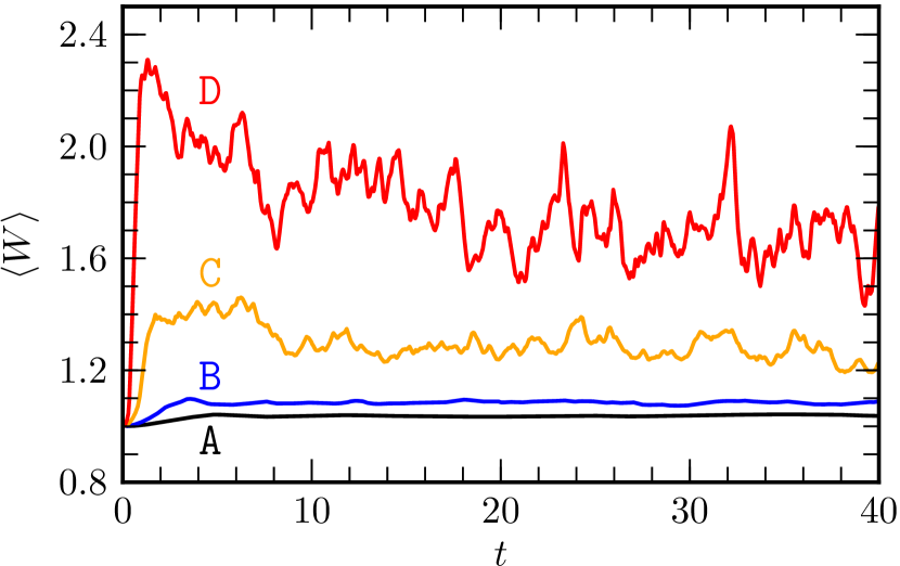
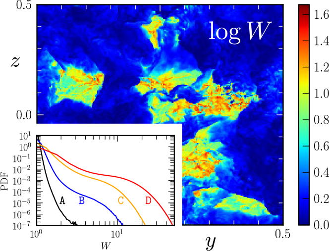
Figure 1.: Left panel: average Lorentz factor as a function of time for the different models considered. Note that a quasi-stationary state is reached before $t\sim 10$ for all values of the driving force. Right panel: logarithm of the Lorentz factor on the $(y,z)$ plane at the final time of model D. Note the large spatial variations of the Lorentz factor with front-like structures. The time-averaged PDFs are shown in the lower left corner for the different models considered.

The set of relativistic-hydrodynamic equations is closed by the equation of state (EOS) $p=\frac{1}{3}\rho$, thus modelling a hot, optically-thick, radiation-pressure dominated plasma, such as the electron-positron plasma in a GRB fireball or the matter in the radiation-dominated era of the early Universe. The EOS used can be thought as the relativistic equivalent of the classical isothermal EOS in that the sound speed is a constant, i.e. $c_{s}^{2}=1/3$. At the same time, an ultrarelativistic fluid is fundamentally different from a classical isothermal fluid. For instance, its “inertia” is entirely determined by the temperature and the notion of rest-mass density is lost since the latter is minute (or zero for a pure photon gas) when compared with the internal one. For these reasons, there is no direct classical counterpart of an ultrarelativistic fluid and a relativistic description is needed even for small velocities.

We solve the equations of relativistic hydrodynamics in a 3D periodic domain using the high-resolution shock capturing scheme described in (Radice & Rezzolla 2012). In particular, ours is a flux-vector-splitting scheme (Toro 1999), using the fifth-order MP5 reconstruction (Suresh & Huynh 1997), in local characteristic variables (Hawke 2001), with a linearized flux-split algorithm with entropy and carbuncle fix
(Radice & Rezzolla 2012).

3 Basic flow properties

Our analysis is based on the study of four different models, which we label as A, B, C and D, and which differ for the initial amplitude of the driving factor $\tilde{F}=1,2,5$ for models A–C, and $\tilde{F}(t)=10+\frac{1}{2}t$ for the extreme model D. Each model was evolved using three different uniform resolutions of $128^{3}$, $256^{3}$ and $512^{3}$ grid-zones over the same unit lengthscale. As a result, model A is subsonic, model B is transonic and models C and D are instead supersonic. The spatial and time-averaged relativistic Mach numbers $\langle vW\rangle/(c_{s}W_{s})$ are $0.362$, $0.543$, $1.003$ and $1.759$ for our models A, B, C and D, while the average Lorentz factors are $1.038$, $1.085$, $1.278$ and $1.732$ respectively

The initial conditions are simple: a constant energy density and a zero-velocity field. The forcing term, which is enabled at time $t=0$, quickly accelerates the fluid, which becomes turbulent. By the time when we start to sample the data, i.e. at $t=10$ (light-)crossing times, turbulence is fully developed and the flow has reached a stationary state. The evolution is then carried out up to time $t=40$, thus providing data for 15, equally-spaced timeslices over $30$ crossing times. As a representative indicator of the dynamics of the system, we show in the left panel of Fig. 1 the time evolution of the average Lorentz factor for the different models considered. Note that the Lorentz factor grows very rapidly during the first few crossing times and then settles to a quasi-stationary evolution. Furthermore, the average grows nonlinearly with the increase of the driving term, going from $\langle W\rangle\simeq 1.04$ for the subsonic model A, up to $\langle W\rangle\simeq 1.73$ for the most supersonic model D.

The probability distribution functions (PDFs) of the Lorentz factor are shown in the right panel of Fig. 1 for the different models. Clearly, as the forcing is increased, the distribution widens, reaching Lorentz factors as large as $W\simeq 40$ (i.e. to speeds $v\simeq 0.9997$). Even in the most “classical” case A, the flow shows patches of fluid moving at ultrarelativistic speeds. Also shown in Fig. 1 is the logarithm of the Lorentz factor on the $(y,z)$ plane and at $t=40$ for model D, highlighting the large spatial variations of $W$ and the formation of front-like structures.

4 Universality

As customary in studies of turbulence, we have analyzed the power spectrum of the velocity field

$$E_{\bm{v}}(k)\equiv\frac{1}{2}\int_{|\bm{k}|=k}|\hat{\bm{v}}(\bm{k})|^{2}\,d\bm{k}\,,$$ (3)

where $\bm{k}$ is a wavenumber three-vector and

$$\hat{\bm{v}}(\bm{k})\equiv\int_{V}\bm{v}(\bm{x})e^{-2\pi i\bm{k}\cdot\bm{x}}\,d\bm{x}\,,$$ (4)

with $V$ being the three-volume of our computational domain. A number of recent studies have analyzed the scaling of the velocity power spectrum in the inertial range, that is, in the range in wavenumbers between the lengthscale of the problem and the scale at which dissipation dominates. More specifically, Inoue et al. (2011) has reported evidences of a Kolmogorov $k^{-5/3}$ scaling in a freely-decaying MHD turbulence, but has not provided a systematic convergence study of the spectrum. Evidences for a $k^{-5/3}$ scaling were also found by Zhang et al. (2009), in the case of the kinetic-energy spectrum, which coincides with the velocity power-spectrum in the incompressible case. Finally, Zrake & MacFadyen (2012) has performed a significantly more systematic study for driven, transonic, MHD turbulence, but obtained only a very small (if any) coverage of the inertial range.

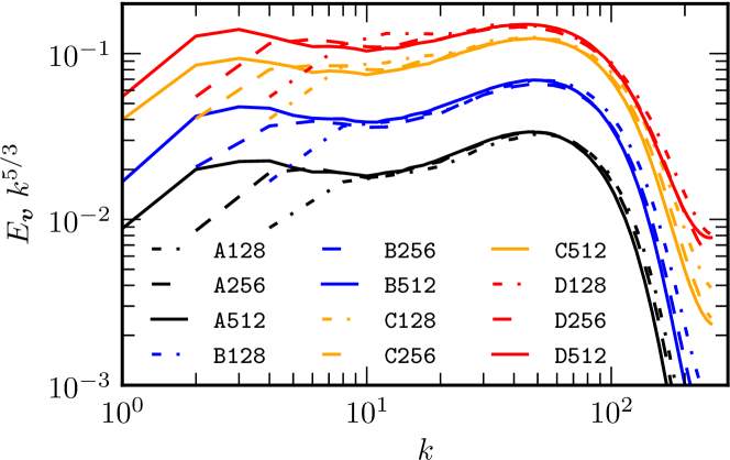
Figure 2.: Power spectra of the velocity field. Different lines refer to the three resolutions used and to the different values of the driving force. The spectra are scaled assuming a $k^{-5/3}$ law.

The time-averaged velocity power spectra computed from our simulations are shown in Fig. 2. Different lines refer to the three different resolutions used, $128^{3}$ (dash-dotted), $256^{3}$ (dashed) and $512^{3}$ (solid lines), and to the different values of the driving force. To highlight the presence and extension of the inertial range, the spectra are scaled assuming a $k^{-5/3}$ law, with curves at different resolutions shifted of a factor two or four, and nicely overlapping with the high-resolution one in the dissipation region. Overall, Fig. 2 convincingly demonstrates the good statistical convergence of our code and gives a strong support to the idea that the key prediction of the Kolmogorov model (K41) (Kolmogorov 1991) carries over to the relativistic case. Indeed, not only does the velocity spectrum for our subsonic model A shows a region, of about a decade in length, where the $k^{-5/3}$ scaling holds, but this continues to be the case even as we increase the forcing and enter the regime of relativistic supersonic turbulence with model D. In this transition, the velocity spectrum in the inertial range, the range of lengthscales where the flow is scale-invariant, is simply “shifted upwards” in a self-similar way, with a progressive flattening of the bottleneck region, the bump in the spectrum due to the non-linear dissipation introduced by our numerical scheme. Steeper scalings, such as the Burger one, $k^{-2}$, are also clearly incompatible with our data.

All in all, this is one of our main results: the velocity power spectrum in the inertial range is universal, that is, insensitive to relativistic effects, at least in the subsonic and mildly supersonic cases. Note that this does not mean that relativistic effects are absent or can be neglected when modelling relativistic turbulent flows.

5 Intermittency

Not all of the information about relativistic turbulent flows is contained in the velocity power spectrum. Particularly important in a relativistic context is the intermittency of the velocity field, that is, the local appearance of anomalous, short-lived flow features, which we have studied by looking at the parallel-structure functions of order $p$

$$S^{\parallel}_{p}(r)\equiv\big{\langle}|\delta_{r}v|^{p}\big{\rangle},\qquad\delta_{r}v=\big{[}\bm{v}(\bm{x}+\bm{r})-\bm{v}(\bm{x})\big{]}\cdot\frac{\bm{r}}{r}$$ (5)

where $\bm{r}$ is a vector of length $r$ and the average is over space and time.

Model A
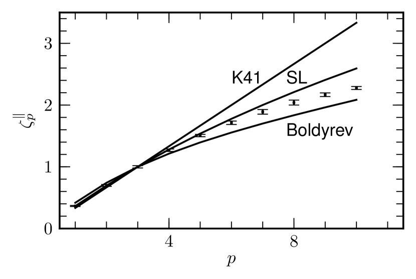
  Model C

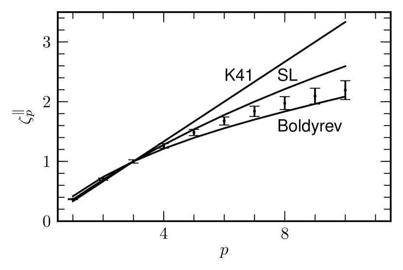
Model B
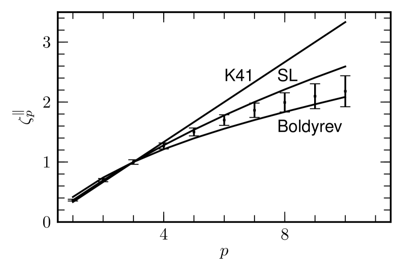
  Model D

Figure 3.: Structure function exponents as computed using the ESS technique for different models. Also shown in the Figure are the analytic predictions from two classical intermittency models: the She and Leveque (SL) (She & Leveque 1994) and the Boldyrev (Boldyrev 2002) models.

The scaling exponents of the parallel structure functions, i.e. $\zeta^{\parallel}_{p}$ s.t. $S_{p}^{\parallel}(r)\sim r^{\zeta^{\parallel}_{p}}$, have been computed up to $p=10$ using the extended-self-similarity (ESS) technique (Benzi et al. 1993) and are summarized in Figure 3. The errors are estimated by computing the exponents without the ESS or using only the data at the final time. We also show the values as computed using the classical K41 theory, as well as using the estimates by She and Leveque (SL) (She & Leveque 1994) for incompressible turbulence, i.e. $\zeta^{\parallel}_{p}=\frac{p}{9}+2-2(\frac{2}{3})^{p/3}$, and those by Boldyrev (Boldyrev 2002) for Kolmogorov-Burgers supersonic turbulence, i.e. $\zeta^{\parallel}_{p}=\frac{p}{9}+1-(\frac{1}{3})^{p/3}$.

Not surprisingly, as the flow becomes supersonic, the high-order exponents tend to flatten out and be compatible with the Boldyrev scaling, as the most singular velocity structures become two-dimensional shock waves. $\zeta_{2}^{\parallel}$, instead, is compatible with the She-Leveque model even in the supersonic case. This is consistent with the observed scaling of the velocity power spectrum, which presents only small intermittency corrections to the $k^{-5/3}$ scaling. Previous classical studies of weakly compressible (Benzi et al. 2008) and supersonic turbulence (Porter et al. 2002) found the scaling exponents to be in very good agreement with the ones of the incompressible case and to be well described by the SL model. This is very different from what we observe even in our subsonic model A, in which the exponents are significantly flatter than in the SL model, suggesting a stronger intermittency correction. This deviation is another important result of our simulations.

6 Conclusions

Using a series of high-order direct numerical simulations of driven relativistic turbulence in a hot plasma, we have explored the statistical properties of relativistic turbulent flows with average Mach numbers ranging from $0.4$ to $1.7$ and average Lorentz factors up to $1.7$. We have found that relativistic effects enhance significantly the intermittency of the flow and affect the high-order statistics of the velocity field. Nevertheless, the low-order statistics appear to be universal, i.e. independent from the Lorentz factor, and in good agreement with the classical Kolmogorov theory.

Acknowledgments

We thank M.A. Aloy, P. Cerdá-Durán, and M. Obergaulinger for discussions. The calculations were performed on the clusters at the AEI and on the SuperMUC cluster at the LRZ. Partial support comes from the DFG grant SFB/Trans-regio 7 and by “CompStar”, a Research Networking Programme of the ESF.

References

- Benzi et al. (2008) Benzi, R., Biferale, L., Fisher, R., Kadanoff, L., Lamb, D., & Toschi, F. 2008, Phys. Rev. Lett., 100, 1
- Benzi et al. (1993) Benzi, R., Ciliberto, S., Tripiccione, R., Baudet, C., Massaioli, F., & Succi, S. 1993, Phys. Rev. E, 48, 29
- Boldyrev (2002) Boldyrev, S. 2002, The Astrophysical Journal, 569, 841
- Font (2008) Font, J. A. 2008, Living Rev. Relativ., 6, 4. 0704.2608.
- Hawke (2001) Hawke, I. 2001, Ph.D. thesis, University of Cambridge
- Inoue et al. (2011) Inoue, T., Asano, K., & Ioka, K. 2011, Astrophys. J., 734, 77
- Kolmogorov (1991) Kolmogorov, A. N. 1991, Proceedings of the Royal Society A: Mathematical, Physical and Engineering Sciences, 434, 9
- Porter et al. (2002) Porter, D., Pouquet, A., & Woodward, P. 2002, Phys. Rev. E, 66, 1
- Radice & Rezzolla (2012) Radice, D., & Rezzolla, L. 2012, Astronomy and Astrophysics. In press, 1206.6502
- Radice & Rezzolla (2012) Radice, D., & Rezzolla, L. 2012, Submitted. 1209.2936
- She & Leveque (1994) She, Z., & Leveque, E. 1994, Phys. Rev. Lett., 72, 336
- Suresh & Huynh (1997) Suresh, A., & Huynh, H. T. 1997, Journal of Computational Physics, 136, 83
- Toro (1999) Toro, E. F. 1999, Riemann Solvers and Numerical Methods for Fluid Dynamics (Springer-Verlag)
- Zhang et al. (2009) Zhang, W., MacFadyen, A., & Wang, P. 2009, Astrophys. J., 692, L40. 0811.3638
- Zrake & MacFadyen (2012) Zrake, J., & MacFadyen, A. I. 2012, Astrophys. J., 744, 32. 1108.1991