Efficient implementation of finite element methods on non-matching and overlapping meshes in 3D

Abstract

In recent years, a number of finite element methods have been formulated for the solution of partial differential equations on complex geometries based on non-matching or overlapping meshes. Examples of such methods include the fictitious domain method, the extended finite element method, and Nitsche’s method. In all of these methods, integrals must be computed over cut cells or subsimplices which is challenging to implement, especially in three space dimensions. In this note, we address the main challenges of such an implementation and demonstrate good performance of a fully general code for automatic detection of mesh intersections and integration over cut cells and subsimplices. As a canonical example of an overlapping mesh method, we consider Nitsche’s method which we apply to Poisson’s equation and a linear elastic problem.

1 Introduction

A fundamental problem in computational science is to develop methods for the solution of partial differential equations on domains containing one or several objects that may have complex or time-dependent geometry. One approach to attacking this problem is to allow overlapping meshes where a mesh representing an object is allowed to overlap a background mesh representing the surroundings of the object; see for instance Chesshire and Henshaw [22], Yu [60], Zhang et al. [61], Mayer et al. [50] for various applications.

In solid mechanics, overlapping meshes may be used to represent materials consisting of elastic objects inserted into a surrounding elastic material of another type [37], and in fluid–structure interaction, an overlapping mesh may be used to represent an elastic body immersed in a fluid represented by a fixed background mesh [60, 7, 49]. Another common application [22, 26, 25] is found in mesh generation where a complicated geometry such as, for example, a pipe junction, may be decomposed into simpler parts and one unstructured tetrahedral mesh is created for each part. These components may then be stored, reused and recombined in applications by using an overlapping mesh technique.

Overlapping mesh techniques are of particular interest in simulations that involve moving objects. For such problems, overlapping mesh techniques are an attractive alternative to ALE techniques. The main advantage is that by using an overlapping mesh technique, one avoids deformation of the mesh that may lead to deterioration of the mesh quality and ultimately force remeshing. This is of particular importance in the simulation of fluid–structure interaction where the topology of the fluid domain may change due to deformation of the solid.

The main focus of this work is on the general algorithms and efficient implementation that is required to handle complex problems posed on overlapping meshes in three space dimensions. Many of the presented algorithms and the tools developed are of interest and use for the implementation of various overlapping mesh techniques. To make the discussion concrete, we here focus mainly on Nitsche’s method. In  Hansbo et al. [33], a consistent finite element method for overlapping meshes based on Nitsche’s method was introduced and analyzed. The basic idea is to construct a finite element space by taking the direct sum of the space of continuous piecewise polynomial functions on the overlapping mesh and the restriction of the space of continuous piecewise polynomial functions to the complement of the overlapping mesh, and then impose the interface conditions using Nitsche’s method. It was shown that this approach leads to a stable method of optimal order for arbitrary degree polynomial approximation.

The main challenge in the implementation is to compute the intersection between the overlapping and the background mesh. The result is a set of cut cells which may be arbitrarily complex polyhedra. These arise as the result of subtracting from the tetrahedra of the background mesh a set of tetrahedra from the overlapping mesh. By adopting algorithms and search structures from the field of computational geometry, we show how these issues can be handled in an efficient manner. Furthermore, one needs to compute integrals on the resulting polyhedra. This can be carried out efficiently based on an application of the divergence theorem in combination with potentials to represent an integral on the three-dimensional polyhedron as a sum of one-dimensional integrals on its edges.

The presented algorithms and implementation are relevant for several other types of related methods, including the extended finite element method (XFEM) [58, 31], non-fitted sharp interface methods [32, 14], and mesh-tying techniques [25].

1.1 Major contributions of this paper

Our work consists of several contributions. We identify the major techniques used in the implementation of overlapping mesh methods and related methods. We further identify useful data structures and algorithms from the field of computational geometry. As part of our work, existing computational geometry libraries such as CGAL [1] and GTS [2] have been wrapped into the general purpose finite element library DOLFIN [43] and into an extension library on top of it, thereby making these algorithms and data structures more easily accessible to the finite element community. Based on our implementation, we demonstrate for the first time a highly efficient implementation of Nitsche’s method on overlapping meshes for several problems posed in three spatial dimensions, thus opening the possibility of employing Nitsche-based overlapping mesh methods for challenging 3D problems such as fluid–structure interaction or domain-bridging problems.

1.2 Outline of this paper

In Section 2, we review Nitsche’s overlapping mesh method for a model problem and present in Section 3 the techniques and algorithms we have developed for efficient implementation of Nitsche’s method in three space dimensions. The corresponding implementation and data structures are described in Section 4. Finally, we present in Section 5 numerical examples that demonstrate the convergence of the numerical solution as well as the scaling of the work required to compute mesh intersections relative to standard finite element assembly on matching meshes.

2 Nitsche’s method on overlapping meshes

We here review Nitsche’s method for a simple model problem posed on two overlapping meshes.

2.1 Model problem

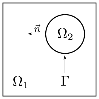
Fig. 1: Two domains $\Omega_{1}$ and $\Omega_{2}$ separated by the common interface $\Gamma=\partial\Omega_{1}\cap\partial\Omega_{2}$.

Let $\Omega_{0}=(\overline{\Omega_{1}\cup\Omega_{2}})^{\circ}$ be a domain in $\mathbb{R}^{3}$, with boundary $\partial\Omega_{0}$, consisting of two (open and bounded) subdomains $\Omega_{1}$ and $\Omega_{2}$ separated by the interface $\Gamma=\partial\Omega_{1}\cap\partial\Omega_{2}$. We consider the following elliptic model problem: find $u:\Omega_{0}\rightarrow\mathbb{R}$ such that

$$-\Delta u_{i} =f_{i} \text{in }\Omega_{i},\quad i=1,2,$$ (1)

$$[\nabla u\cdot\mathbf{n}] =0 \text{on }\Gamma,$$ (2)

$$[u] =0 \text{on }\Gamma,$$ (3)

$$u =0 \text{on }\partial\Omega_{0,\mathrm{D}}{},$$ (4)

$$\nabla u\cdot\mathbf{n} =g \text{on }\partial\Omega_{0,\mathrm{N}}{}.$$ (5)

We here use the notation $v_{i}=v|_{\Omega_{i}}$ for the restriction of a function $v$ to the subdomain $\Omega_{i}$ for $i=1,2$, $\mathbf{n}$ is the unit normal to $\Gamma$ directed from $\Omega_{2}$ into $\Omega_{1}$, and $[v]=v_{2}-v_{1}$ denotes the jump in a function over the interface $\Gamma$. In addition, the boundary $\partial\Omega_{0}$ is divided into two subdomains $\partial\Omega_{0,\mathrm{D}}{}$ and $\partial\Omega_{0,\mathrm{N}}{}$ where Dirichlet and Neumann boundary conditions are applied, respectively.

2.2 Finite element formulation

We consider a situation where a background mesh $\mathcal{T}_{0}$ is given for $\Omega_{0}=(\overline{\Omega_{1}\cup\Omega_{2}})^{\circ}$ and another mesh $\mathcal{T}_{2}$ is given for the overlapping domain $\Omega_{2}$ (see Figure 1). Both meshes are assumed to consist of shape-regular tetrahedra $T$. The mesh $\mathcal{T}_{1}$ covering $\Omega_{1}=(\Omega_{0}\setminus\Omega_{2})^{\circ}$ is constructed by

$$\mathcal{T}_{1}=\{T\cap\Omega_{1}:T\in\mathcal{T}_{0}\wedge|T\cap\Omega_{1}|>0\}.$$ (6)

Note that the $\mathcal{T}_{1}$ consists of both regular and cut elements since the mesh $\mathcal{T}_{0}$ is not a conform tetrahedralization of the subdomain $\Omega_{1}$ in general. For a cut element $T\cap\Omega$, the degree of freedoms are defined to be the same as for the original uncut element $T$. This is illustrated in Figure 2.

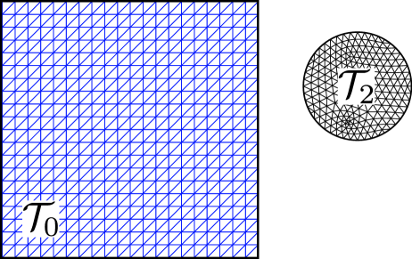
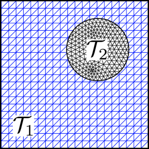
Fig. 2: The mesh $\mathcal{T}_{1}$ for $\Omega_{1}=(\Omega_{0}\setminus\Omega_{2})^{\circ}$ is constructed as the set of cells of $\mathcal{T}_{0}$ not completely overlapped by the cells of $\mathcal{T}_{2}$.

We let ${V}_{h,i}$ denote the space of continuous piecewise fixed-order polynomials on $\mathcal{T}_{i}$ that vanish on $\partial\Omega_{i}\cap\partial\Omega_{0,\mathrm{D}}{}$ for $i=0,2$. The space $V_{h,1}$ is constructed as the restriction to $\Omega_{1}$ of functions in $V_{h,0}$; that is, $V_{h,1}=\{v|_{\Omega_{1}}:v\in V_{h,0}\}$. We may then define a finite element space for the whole domain $\Omega_{0}$ by

$${W}_{h}={V}_{h,1}\bigoplus{V}_{h,2}.$$ (7)

Nitsche’ method proposed by Hansbo et al. [33] then takes the form: find ${u}_{h}\in{W}_{h}$ such that

$$a({u}_{h},{v})=l({v})\quad\forall\,{v}\in{W}_{h},$$ (8)

where

$$a(u,v) =\sum_{i=1,2}\int_{\Omega_{i}}\nabla u\cdot\nabla{v}\,\mathrm{d}x$$ (9)

$$\qquad-\underbrace{\int_{\Gamma}\langle\nabla u\cdot{\mathbf{n}}\rangle[{v}]\,\mathrm{d}S}_{\text{Consistency}}-\underbrace{\int_{\Gamma}\langle\nabla v\cdot{\mathbf{n}}\rangle[u]\,\mathrm{d}S}_{\text{Symmetrization}}+\underbrace{\gamma\int_{\Gamma}h^{-1}[{u}]\cdot[{v}]\,\mathrm{d}S}_{\text{Penalty/Stabilization}},$$

$$l(v) =\int_{\Omega}fv\,\mathrm{d}x+\int_{\partial\Omega_{0,\mathrm{N}}{}}gv\,\mathrm{d}s.$$ (10)

Here, $\gamma$ is a positive penalty parameter and the average $\langle\nabla v\cdot{\mathbf{n}}\rangle$ is chosen to be the one-side derivative $\langle\nabla v\cdot{\mathbf{n}}\rangle=\nabla v_{2}\cdot\mathbf{n}$ according to Hansbo et al. [33]. But as pointed out by the authors, any convex combination of the normal derivatives leads to a consistent formulation.

2.3 Summary of theoretical results

When the penalty parameter $\gamma$ in (9) is chosen large enough, the form $a(\cdot,\cdot)$ is coercive on the discrete space ${W}_{h}$ and one can derive optimal order a priori error estimates in both the energy norm and the $L^{2}$ norm for polynomials of arbitrary degree $p$. The estimates take the form

$$\left(\sum_{i=1}^{2}\|\nabla(u-u_{h})\|^{2}_{\Omega_{i}}+h^{-1}\|[u_{h}]\|_{\Gamma}^{2}\right)^{\frac{1}{2}}\leq Ch^{p}\|u\|_{\Omega_{0},p+1},$$ (11)

$$\|u-u_{h}\|\leq Ch^{p+1}\|u\|_{\Omega_{0},p+1}.$$ (12)

See Hansbo et al. [33] for details. Here, $\|\cdot\|_{\Omega_{0},s}$ denotes the standard Sobolev norm of order $s>0$ on $\Omega_{0}$. A posteriori error estimates and adaptive algorithms are also presented in Hansbo et al. [33].

As observed by Areias and Belytschko [6], Nitsche’s method for an arbitrary cutting interface as in Hansbo and Hansbo [32, 34] can be reinterpreted as a particular instance of an extended finite element method. In contrast, the presented formulation on overlapping meshes lacks such a reinterpretation since two unrelated meshes are involved and therefore the discontinuity across the interface cannot be modeled by the enrichment of degrees of freedom within a single cell. Nevertheless, both methods share some features, especially with regard to their implementation.

3 Techniques and algorithms

The main challenges in the implementation of Nitsche’s method on overlapping meshes arise from the geometric computations which are necessary to assemble the discrete system associated with (8)–(10). Naturally, these geometric computations are more involved in 3D than in 2D. Similar challenges are encountered in related methods such as the extended finite element method [31], but also for the simulation of contact mechanics [59]. Different solutions have been proposed, see for example Sukumar et al. [58] in the case of extended finite elements methods, and Yang and Laursen [59] for contact problems. Here, we take another approach which efficiently solves the issues in the case of the Nitsche overlapping mesh method. In the following, we will first discuss the challenges and their remedies in general terms, and then return to the specific details of our implementation in Section 4.

3.1 Assembly on overlapping meshes

The main implementation challenges arise from the fact that the interface $\Gamma$ can cross the overlapped mesh $\mathcal{T}_{0}$ in an arbitrary manner, which has two consequences. First, the definition of the finite element space (7) involves the restriction of the function space $V_{h,0}$, defined on the full background mesh $\mathcal{T}_{0}$ of $\Omega_{0}$, to the domain $\Omega_{1}$. The restriction results in non-standard element geometries along the interface $\Gamma$ as it can be observed from the definition 6 of $\mathcal{T}_{1}$. Secondly, the weak imposition of the interface conditions (2) and (3) by the interface integrals in (9) involves finite element spaces defined on two unrelated meshes. Both make the assembly challenging to implement, compared to a standard finite element method.

To better understand what kinds of challenges the Nitsche overlapping mesh method adds, we briefly recall the general theme of the assembly routine as it is realized nowadays in many finite element frameworks; see, e.g., Logg [41], Bastian et al. [12]. Nitsche’s method is closely related to the classical discontinuous Galerkin (DG) methods, which makes it natural to depart from the assembly in the DG case. A detailed description of finite element assembly for discontinuous Galerkin methods can be found in Ølgaard et al. [55]. We assume a variational problem of the following form: find $u_{h}\in V_{h}$ such that

$$a(u_{h},v)=l(v)\quad\forall\,v\in\hat{V}_{h},$$ (13)

where $a$ and $l$ are bilinear and linear forms, respectively, and $V_{h}$ and $\hat{V}_{h}$ are the discrete trial and test spaces, respectively. For simplicity, we here make the assumption $V_{h}=\hat{V}_{h}$. The solution of the variational problem (13) may then be computed by solving the linear system

$$AU=b,$$ (14)

for $U\in\mathbb{R}^{N}$, with stiffness matrix $A_{IJ}=a(\phi_{J},{\phi}_{I})$ and load vector $b_{I}=l({\phi}_{I})$. Here, $\{\phi_{I}\}_{I=1}^{N}$ denotes a basis for $V_{h}$. During assembly of the tensors $A$ and $b$, one usually iterates over all cells $T\in\mathcal{T}$ and computes the contributions from each cell as the cell tensors $A^{T}_{ij}=a(\phi_{j}^{T},\phi_{i}^{T})$ and $b^{T}_{i}=l({\phi}_{i})$ where $\{\phi^{T}_{i}\}_{i=1}^{n}$ is the local finite element basis on $T$ (the shape functions). The element tensors are then scattered into the global tensors $A$ and $b$ by adding the entries according to a given local-to-global mapping $\iota_{T}:i\mapsto I$. One may similarly add contributions from each facet $F$ of the set of boundary facets $\partial_{e}T$ (the set of exterior facets) and, for the implementation of a DG method, from each facet $F$ of the set of interior facets $\partial_{i}T$. Algorithm 1 summarizes the parts of the standard assembly algorithm relevant for our discussion.

$A=0$

for each $T\in\mathcal{T}$:

$\mathcal{I}(T)=\{1,\dots,\text{dim}(\hat{V}_{h}(T))\}\times\{1,\dots,\text{dim}(V_{h}(T))\}$

for each $(i,j)\in\mathcal{I}(T):$

$A^{T}_{ij}=a(\phi^{T}_{j},\hat{\phi}^{T}_{i})$

for each $(i,j)\in\mathcal{I}(T):$

$A_{\hat{\iota}_{T}(i),\iota_{T}(j)}+=A^{T}_{ij}$

for each $F\in\partial_{e}\mathcal{T}$:

$\mathcal{I}_{e}(F)=\{1,\dots,\text{dim}(\hat{V}_{h}^{e}(F))\}\times\{1,\dots,\text{dim}(V_{h}^{e}(F))\}$

for each $(i,j)\in\mathcal{I}_{e}(F)$:

$A^{T}_{ij}=a(\phi^{F,e}_{j},\hat{\phi}^{F,e}_{i})$

for each $(i,j)\in\mathcal{I}_{e}(F)$:

$A_{\hat{\iota}_{F}^{e}(i),\iota^{e}_{F}(j)}+=A^{T}_{ij}$

for each $F\in\partial_{i}\mathcal{T}$:

$\mathcal{I}_{i}(F)=\{1,\dots,\text{dim}(\hat{V}_{h}^{i}(F))\}\times\{1,\dots,\text{dim}(V_{h}^{i}(F))\}$

for each $(i,j)\in\mathcal{I}_{i}(F)$:

$A^{T}_{ij}=a(\phi^{F,i}_{j},\hat{\phi}^{F,i}_{i})$

for each $(i,j)\in\mathcal{I}_{i}(F)$:

$A_{\hat{\iota}^{i}_{F}(i),\iota^{i}_{F}(j)}+=A^{T}_{ij}$

Algorithm 1 Standard finite element assembly of a bilinear form $a(\cdot,\cdot)$. The local finite element spaces are denoted by $V_{h}(T),V_{h}(F)$ etc.

We now consider how the standard assembly algorithm must be modified in the case of Nitsche’s method on overlapping meshes. We first note that the tessellation $\mathcal{T}_{0}$ of the background domain $\Omega_{0}$ may be decomposed into three disjoint subsets:

$$\mathcal{T}_{0}=\mathcal{T}_{0,1}\cup\mathcal{T}_{0,2}\cup\mathcal{T}_{0,\Gamma},$$ (15)

where $\mathcal{T}_{0,1}=\{T\in\mathcal{T}_{0}:T\subset\overline{\Omega}_{1}\}$, $\mathcal{T}_{0,2}=\{T\in\mathcal{T}_{0}:T\subset\overline{\Omega}_{2}\}$, and $\mathcal{T}_{0,\Gamma}=\{T\in\mathcal{T}_{0}:|T\cap\Omega_{i}|>0,\ i=1,2\}$ denote the sets of not, completely and partially overlapped cells relative to $\Omega_{2}$, respectively.

Integrals over the cells of $\mathcal{T}_{0,1}$ can be assembled using a standard assembly algorithm. Furthermore, integrals over the cells of $\mathcal{T}_{0,2}$ need not be assembled (the corresponding contributions will be assembled over $\mathcal{T}_{2}$). However, assembly must be carried out over $\mathcal{T}_{0,\Gamma}$, the partially overlapped cells of $\mathcal{T}_{0}$. For the model problem (8)–(10), this requires the evaluation of integrals of the type

$$\int_{P}\nabla\phi^{T}_{j}\cdot\nabla\phi^{T}_{i}\,\mathrm{d}x\,\text{ and }\,\int_{P}f\phi^{T}_{i}\,\mathrm{d}x,$$ (16)

on cut elements (polyhedra) $P=T\cap\Omega_{1}$ where $T\in\mathcal{T}_{0}$. Examining (8)–(10), we further note that we must assemble the terms

$$-\int_{\Gamma}\langle\nabla\phi_{j}\cdot\mathbf{n}\rangle[\phi_{i}]\,\mathrm{d}S-\int_{\Gamma}\langle\nabla\phi_{i}\cdot\mathbf{n}\rangle[\phi_{j}]\,\mathrm{d}S+\gamma\int_{\Gamma}h^{-1}[\phi_{j}]\cdot[\phi_{i}]\,\mathrm{d}S.$$ (17)

This poses an additional challenge, since the integrands involve products of trial and test functions defined on different meshes. Furthermore, the interface $\Gamma$ consists of a subset of the boundary facets $\partial_{e}\mathcal{T}_{2}$ of $\mathcal{T}_{2}$, but each such facet may intersect several cells of $\mathcal{T}_{0}$. We therefore partition each facet on $\Gamma$ into a set of polygons $\{\Gamma_{kl}\}$ such that each polygon $\Gamma_{kl}$ intersects exactly one cell $T^{2}_{k}$ of the overlapping mesh $\mathcal{T}_{2}$ and one cell $T^{0}_{l}$ of the background mesh $\mathcal{T}_{0}$. This is illustrated in Figure 3. Assembly may then be carried out by summing the contributions from each polygon $\Gamma_{kl}$.

Fig. 3: The overlapping meshes in the intersection zone. The filled circles represent the degrees of freedom on each element (here for a piecewise linear approximation on $\mathcal{T}_{2}$ and piecewise quadratic on $\mathcal{T}_{0}$). The interface $\Gamma$ is partitioned so that each part intersects exactly one cell $T^{2}_{k}$ of the overlapping mesh $\mathcal{T}_{2}$ and one cell $T^{0}_{l}$ of the background mesh $\mathcal{T}_{0}$.

In summary, we identify the following main challenges in the implementation of Nitsche’s method on overlapping meshes:

1. collision detection: to determine which cells are involved in the intersection between the two meshes;

2. mesh intersection: to compute the cut cells of the background mesh $\mathcal{T}_{0}$ represented by the polyhedra $\{P^{0}_{l}\}$ and the intersection interface represented by the polygons $\{\Gamma_{kl}\}$;

3. integration on complex polyhedra: to compute integrals on the polyhedra $\{P^{0}_{l}\}$ (and the polygons $\{\Gamma_{kl}\}$).

In the following, we discuss these challenges in some detail and introduce concepts, data structures and algorithms to handle them in an efficient manner. We emphasize that the proposed solutions are not limited to the implementation of Nitsche-type methods, but may also be used for the implementation of related overlapping mesh methods.

3.2 Collision detection

Topological relations between entities of a single mesh can be described by concepts of connectivity or mesh incidence as presented in Logg [42] and Bastian et al. [11]. To represent the topological relation between two overlapping (colliding) meshes, we enrich the notation of Logg [42] by the concepts of collision relations and collision maps. The collision relation $\mathcal{T}_{0}\leftrightarrow\partial\mathcal{T}_{2}$ between $\mathcal{T}_{0}$ and $\partial\mathcal{T}_{2}$ is defined by

$$\mathcal{T}_{0}\leftrightarrow\partial\mathcal{T}_{2}=\{(i,j):T_{i}\cap F_{j}\neq\emptyset\wedge T_{i}\in\mathcal{T}_{0}\wedge F_{j}\in\partial\mathcal{T}_{2}\}.$$ (18)

The collision relation lists pairs of indices of all intersecting cells of the background mesh $\mathcal{T}_{0}$ with boundary facets of the overlapping mesh $\mathcal{T}_{2}$. Furthermore, each index of an intersected entity is mapped to the set of indices of intersecting entities via a pair of collision maps:

$$(\mathcal{T}_{0}\to\partial\mathcal{T}_{2})(i)=\{j:(i,j)\in\mathcal{T}_{0}\leftrightarrow\partial\mathcal{T}_{2}\},$$ (19)

$$(\partial\mathcal{T}_{2}\to\mathcal{T}_{0})(j)=\{i:(i,j)\in\mathcal{T}_{0}\leftrightarrow\partial\mathcal{T}_{2}\}.$$ (20)

We note that the collision maps $\mathcal{T}_{0}\to\partial\mathcal{T}_{2}$ and $\partial\mathcal{T}_{2}\to\mathcal{T}_{0}$ can be computed from the collision relation $\mathcal{T}_{0}\leftrightarrow\partial\mathcal{T}_{2}$.

A naive approach to computing the collision relation between two meshes $\mathcal{T}_{0}$ and $\mathcal{T}_{2}$ would be to intersect each cell of $\mathcal{T}_{0}$ with each cell of $\mathcal{T}_{2}$, resulting in an $\mathcal{O}(|\mathcal{T}_{0}|\cdot|\mathcal{T}_{2}|)$-complexity, which is not feasible for large meshes. However, efficient algorithms and data structures which reduce the complexity dramatically have been developed in the fields of computer science, computational geometry, and computer graphics. The task of determining whether two objects collide arises naturally in the rendering of a computer game and the objects in question are often represented by meshes. In this paper, we limit the description to those techniques used in our work and refer to the books Ericson [27], Schneider and Eberly [57], and Akenine-Möller et al. [3] for a broader overview. To efficiently find all pairs of the collision relation $\mathcal{T}_{0}\leftrightarrow\partial\mathcal{T}_{2}$, two important concepts are used: (i) fast intersection tests for pairs of simple geometric objects and (ii) spatial data structures for large sets of objects to accelerate collision queries.

3.2.1 Fast intersection detection

Fast intersection detection for simple geometric entities such as triangles and tetrahedra is based on so-called geometric predicates. Geometric predicates are tests which determine whether two geometric entities do intersect (collide) without computing the actual intersection. See Figure 4 for an example. This saves work since the actual intersection does not need to be computed when the geometric predicate is false.

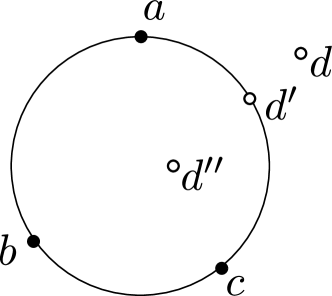
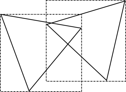
Fig. 4: (Left) A typical example of a geometric predicate is the incircle test, which tells whether a given point $d$ lies on the inside, on the outside, or on a circle defined by three points $a,\ b,\ c$. (Right) Axis aligned bounding boxes (AABB) of two triangles.

3.2.2 Spatial data structures

Spatial data structures provide a hierarchical ordering of geometric objects, which allows quick traversal of large sets of geometric objects as part of a collision test. There exist two principal approaches based on either space subdivisions or bounding volume hierarchies, which can both be realized as tree-like data structures. As the name indicates, subdivision approaches rely on some sort of geometric subdivision of the entire space embedding the structures of interest, in our case a finite element mesh. Typical examples are binary space partitions (BSP) trees, quadtrees, and octrees. Since the embedding space is subdivided, the leaf of a tree will usually not represent a single mesh entity and therefore further selection procedures are required to determine the actual intersections.

In contrast, a bounding volume hierarchy is a tree which is built from bounding volumes; that is, simple geometric shapes containing the objects to be tested. Examples of such data structures are axis aligned bounding boxes (AABB, see Figures 4 and 5), oriented bounding boxes (OBB) and so-called k-DOPs, discrete orientation polytopes described by $k$ hyperplanes. The purpose of using bounding volumes is twofold: (i) testing for collision of bounding volumes is cheaper than testing for collision of the bounded objects, and (ii) the simple geometry of the bounding volumes means that they can be stored efficiently in a hierarchical manner.

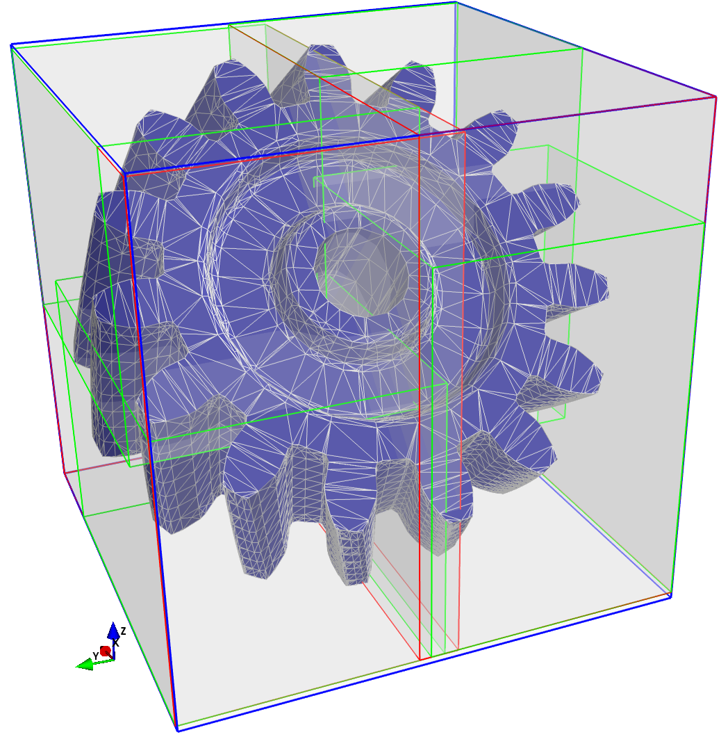
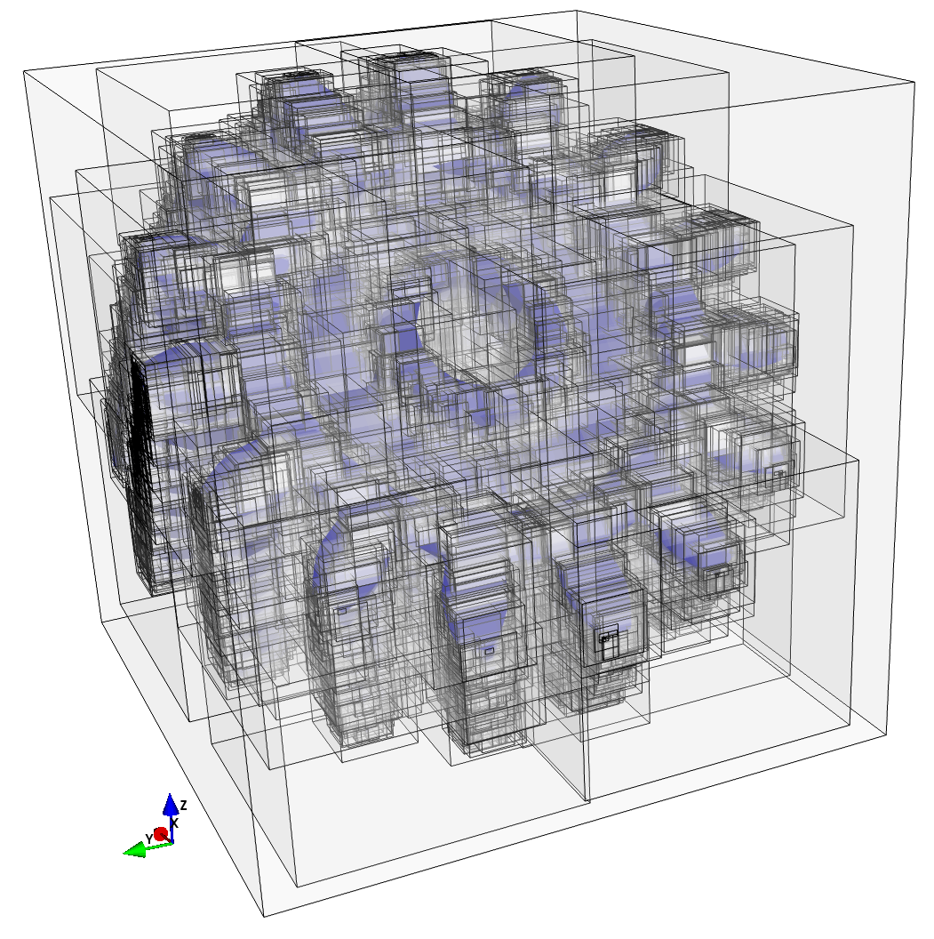
Fig. 5: Bounding volume tree of gear mesh. (Left) Root bounding box (blue) and the next two generations (red and green). (Right) Every fourth level of the complete bounding box tree.

3.2.3 Building the collision map

Bounding volume trees accelerate asymmetric collision queries between a tree embedding a large set of objects and a single simple object like a tetrahedron. The concept becomes even more powerful when intersection tests between two large sets of geometric primitives are desired, as in our case of two meshes. Then a hierarchical traversal of both trees greatly improves the $\mathcal{O}(|\mathcal{T}_{0}|\cdot|\mathcal{T}_{2}|)$-complexity of the naive approach. Algorithm 2 describes how to employ a hierarchical traversal to compute the collision map.

compute_collisions($A$, $B$):

if $A\cap B=\emptyset$:

return

else if is_leaf($A$) $\wedge$ is_leaf($B$):

if $T_{A}\cap T_{B}\neq\emptyset$:

$(i,j)=(\mathrm{index}(T_{A}),\mathrm{index}(F_{B}))$

$\mathcal{T}_{0}\leftrightarrow\partial\mathcal{T}_{2}:=\mathcal{T}_{0}\leftrightarrow\partial\mathcal{T}_{2}\cup(i,j)$

else if descend_a($A$, $B$):

for $a$ $\in$ children($A$):

compute_collisions($a$, $B$)

else:

for $b$ $\in$ children($B$):

compute_collisions($A$, $b$)

descend_a($A$, $B$):

return is_leaf($B$) $\vee\,(\neg$is_leaf($A$) $\wedge\,|A|\geq|B|)$

Algorithm 2 Traversal of two bounding volume trees. Starting from the root of both trees, pairs of nodes are recursively tested for intersection. Only if the bounding volumes $A$ and $B$ of two nodes overlap may the children possibly overlap. A so-called descend rule is applied to decide with which of the two nodes to proceed. A popular and effective rule is to choose the one with the larger volume [27] since it gives the largest volume reduction for subsequent bounding volumes. If two leaf bounding volumes are reached, then the mesh entities bounded by them are tested for intersection.

After the completion of the traversal according to Algorithm 2, which identifies all cells of $\mathcal{T}_{0}$ that intersect the boundary of $\mathcal{T}_{2}$, it remains to check whether the remaining cells (which do not intersect the boundary of $\mathcal{T}_{2}$) are either completely overlapped or not overlapped by $\mathcal{T}_{2}$. To check this, it is enough to take a single point contained in each cell and check whether it is in $\Omega_{2}$. To avoid building a third AABB tree for the entire mesh $\mathcal{T}_{2}$ and to take advantage of the already built tree for $\partial\mathcal{T}_{2}$, one can use a method known as ray-shooting; see Akenine-Möller et al. [3]. The idea is simple: counting how often a ray starting at the point in question intersects the surface $\partial\mathcal{T}_{2}$ tells whether it is inside (odd number of intersections) or outside (even number of intersections). To efficiently find all ray–surface intersections, one may reuse the same AABB tree for $\partial\mathcal{T}_{2}$ that was used in Algorithm 2.

To summarize, the collision map and classification of cells according to the splitting (15) can be found efficiently by utilizing AABB trees, fast traversal of pairs of AABB hierarchies, and ray shooting techniques.

3.3 Mesh intersection

The next step is to compute the cut cells (polyhedra) $\{P^{0}_{l}\}$ and the interface decomposition $\{\Gamma_{kl}\}$; see Figure 3. This computation may be phrased in terms of so-called boolean operations which are widely used in CAD systems to build complex geometries by performing boolean operations between primitives from a finite set of geometries. Algorithm 3 summarizes the use of boolean operations to compute $\{P^{0}_{l}\}$ and $\{\Gamma_{kl}\}$. The resulting geometric objects are depicted in Figure 6.

for each $T\in\mathcal{T}_{0}$ intersected by $\Gamma$:

$l=\mathrm{index}(T)$

$P^{0}_{l}:=T$

$S:=\emptyset$

for each $F\in(\mathcal{T}_{0}\to\partial\mathcal{T}_{2})(l)$:

$S:=S\cup F$

$P^{0}_{l}:=T^{+}_{S}$

for each $F\in\partial\mathcal{T}_{2}$:

$j=\mathrm{index}(F)$

$k=\mathrm{index}(T_{F})$

for each $T\in(\partial\mathcal{T}_{2}\to\mathcal{T}_{0})(j)$:

$l=\mathrm{index}(T)$

$\Gamma_{kl}:=F\cap T$

Algorithm 3 Mesh intersection. Note that the surface $S$ defined by the union of all facets $F$ intersecting the tetrahedron $T$ divides $T$ into two parts $T^{+}_{S}$ and $T^{-}_{S}$ according to orientation of $S$.

The boolean operations are completely delegated to the computational geometry library GTS [2] which uses a so-called ear-clipping algorithm to compute the surface tesselation of the intersection objects. The implemented ear clipping algorithms (first introduced in Fournier and Montuno [28]) are known to have $\mathcal{O}(n\log(n))$ complexity, where $n$ is the number of vertices of the 3D-polygon. This number in turn ($n$) depends on the mesh quality parameters such as the smallest and widest element angles and will in practice be bounded by a constant.

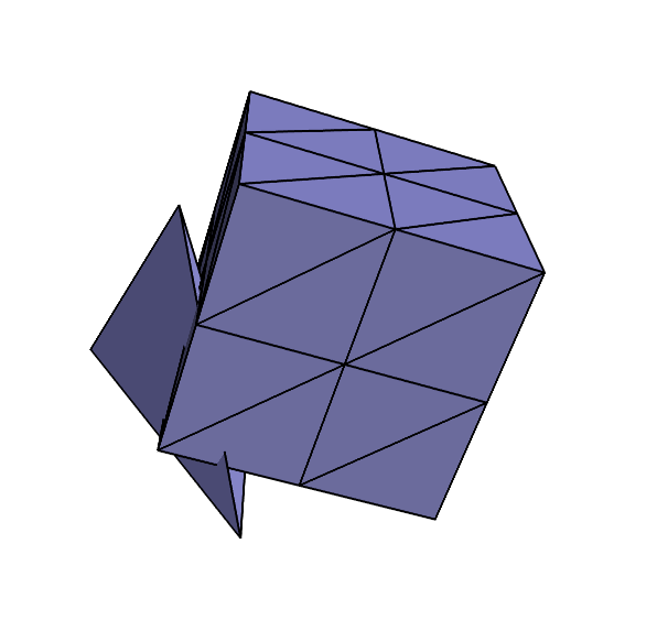
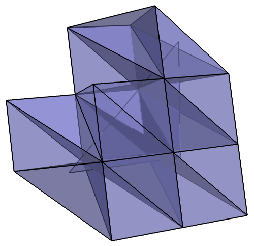
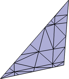
Fig. 6: (Left top) A tetrahedron cell $T^{0}_{l}$ from the background mesh $\mathcal{T}_{0}$ overlapped by a tetrahedral mesh $\mathcal{T}_{2}$ of a cube. (Bottom left) The resulting cut cell (polyhedron) $P^{0}_{l}$. (Top right) An interface facet $F\in\partial\mathcal{T}_{2}$ of the overlapping mesh $\mathcal{T}_{2}$ intersected by a number of tetrahedra from the background mesh $\mathcal{T}_{0}$. (Bottom left) The resulting facet decomposition (triangulation) $\{\Gamma_{kl}\}$.

3.4 Integration on complex polyhedra

The last required step in implementing the overlapping mesh method is to compute the integrals (16) and (17) on the cut cells $\{P^{0}_{l}\}$ and on the interface decomposition $\{\Gamma_{kl}\}$, respectively. A widely used technique in the implementation of the extended finite element method [52, 24, 58, 15] is to decompose a cell into subcells which are aligned with the interface. The interface is either approximated by a plane within the cell [29, 30] or completely recovered [24, 58], even in the case of higher order interfaces [49]. Inside each tetrahedron of the subtetrahedralization, one may then use a standard integration scheme. However, subtetrahedralization of an arbitrary polyhedron is in general a quite challenging problem [56], and its existence cannot even be guaranteed without adding additional vertices [21], in contrast to the two-dimensional case.

Methods for integration over arbitrary polygonal domains without the use of a subtriangulation have recently been presented in Natarajan et al. [53] and incorporated into the extended finite element method with discontinuous enrichments in Natarajan et al. [54]. Using Schwarz–Christoffel conformal mappings as the fundamental tool, the technique is strongly bounded to two space dimensions and hard to generalize to three space dimensions.

We here propose an alternative approach, which is based on a boundary representation of the integrals. Despite the fact that this technique has been known for a long time, see for instance [40], it seems to be largely unknown within the finite element community. Our implementation is based on the efficient realization described in Mirtich [51]. This technique may be easily generalized to the computation of the general moment integral $I_{\alpha}(P)$ over a polyhedron $P$, defined by

$$I_{\alpha}(P)=\int_{P}x^{\alpha}\,\mathrm{d}x=\int_{P}x_{1}^{\alpha_{1}}\cdots x_{d}^{\alpha_{d}}\,\mathrm{d}x,$$ (21)

where $\mathbf{\alpha}=(\alpha_{1},\ldots,\alpha_{d})$ denotes a multi-index of length $d$.

The integral $I_{\alpha}(P)$ is computed in three steps. The first step is to interpret the integrand as the divergence of a polynomial vector field and to rewrite (21) as surface integral:

$$\int_{P}x^{\alpha}\,\mathrm{d}x=\int_{P}\nabla\cdot\sum_{i=1}^{d}\dfrac{x^{\alpha+\mathbf{e}_{i}}}{d(\alpha_{i}+1)}\mathbf{e}_{i}\,\mathrm{d}x=\sum_{F\in\partial P}\sum_{i=1}^{d}\mathbf{n}_{F}\cdot\mathbf{e}_{i}\int_{F}\dfrac{x^{\alpha+\mathbf{e}_{i}}}{d(\alpha_{i}+1)}\,\mathrm{d}s.$$ (22)

Here, $\mathbf{e}_{i}=(0,\ldots,0,1,0,\ldots,0)$ denotes the $i$th unit vector.

Secondly, the plane equation $ax+by+cz=d$ for each facet $F$ allows the construction of a projection map $Z=h(X,Y)$, where $X,Y,Z$ is some positive, orientation-preserving permutation of $x,y,z$. Using the parametrization $h$, one may rewrite the integrals of type $\int_{F}x^{\beta}\,\mathrm{d}s$ in (22) as integrals in the $XY$-plane:

$$\int_{F}x^{\beta}\,\mathrm{d}s=\dfrac{1}{|{n_{Z}}|}\int_{h^{-1}(F)}x(X,Y,h(X,Y))^{\beta}\,\mathrm{d}X\,\mathrm{d}Y.$$ (23)

Here, $n_{Z}$ denotes the $Z$-component of the normal vector $\mathbf{n}_{F}$.

The third step consists of using a parametrization of $\partial h^{-1}(F)$ and Green’s theorem in the plane to rewrite (23) as a sum of line integrals. Together, the three steps reduce the evaluation of the moment integral (21) to the evaluation of a set of one-dimensional integrals with polynomial integrands. We note that the algorithm for the calculation of each moment integral has only a $\mathcal{O}(\#F)$ complexity.

The moment integrals can be used in several ways to finally compute the integrals (16) and (17). First, one may compute the volume and the barycenter as the zeroth and first moments, respectively, which immediately provides a quadrature rule for exact integration of polynomials of degree one. Unfortunately, higher order moments may not be directly reinterpreted as quadrature rules. Furthermore, as the construction of quadrature rules for higher degree polynomials can be quite involved [23], it can be advantageous to avoid run-time generation of quadrature rules. We therefore propose to use the moment integrals $I_{\alpha}(P)$ directly by first interpolating the integrand onto a monomial basis and then summing the contributions:

$$\int_{P}f\,\mathrm{d}x=\int_{P}\sum_{\alpha}f_{\alpha}x^{\alpha}\,\mathrm{d}x=\sum_{\alpha}f_{\alpha}\int_{P}x^{\alpha}\,\mathrm{d}x=\sum_{\alpha}f_{\alpha}I_{\alpha}(P).$$ (24)

Ill-conditioning may be avoided for higher-order expansions by replacing the monomial basis by Bernstein polynomials. In the present work, linear Lagrange elements have been used throughout and so simple barycenter quadrature suffices.

4 Implementation and data structures

We now discuss some of the data structures and classes which reflect the abstract concepts and algorithms described in Section 3. For some of these algorithms, we rely on existing implementations as part of the computational geometry libraries CGAL [1] and GTS [2], while other algorithms have been realized in the finite element library DOLFIN [43, 46] as part of this work. Specialized algorithms for the Nitsche overlapping mesh method have been implemented as part of the extension library DOLFIN-OLM which is built on top of DOLFIN. The code is free/open-source, licensed under the LGPLv3, and available at http://launchpad.net/dolfin-olm.

4.1 The finite element library DOLFIN

Our implementation of Nitsche’s method on overlapping meshes is based on the finite element library DOLFIN which is part of the FEniCS project [44, 41] for automated scientific computing. The main feature of FEniCS is the automated treatment of finite element variational problems, based on automated generation of highly efficient C++ code from abstract high-level descriptions of finite element variational problems expressed in near-mathematical notation [39, 4]. This is combined with built-in tools for working with efficient representations of computational meshes [42] and wrappers for high-performance linear algebra libraries like PETSc [10, 9, 8] and Trilinos [36].

For this work, we have integrated the computational geometry libraries CGAL [1] and GTS [2] with DOLFIN. While CGAL and GTS provide a large part of the functionality needed to compute intersections between tetrahedra, the integration scheme was realized through an adapted version of Mirtich’s code [51]. Furthermore, the assembly routine of DOLFIN was extended to handle integration over cut cells and meshes. Currently, the code for computing local interface integrals has to be implemented manually by the user, but we plan to extend FEniCS, in particular DOLFIN and the form compiler FFC [39, 45], to provide a full automation of Nitsche’s method where a user only needs to supply the abstract variational problem (8).

In the remaining subsections, we present the class abstractions of the algorithms and data structures described in Section 3. These new classes introduced in DOLFIN-OLM allow the implementation of the Nitsche assembly algorithm in a descriptive and concise manner, as illustrated in Figure 7.

 

   

 void NitscheAssembler::assemble_interface(GenericTensor& A, 

   const NitscheForm& a_nit, 

   UFC& ufc_0, 

   UFC& ufc_1) 

 { 

   ... 

   for (CutFacetPartIterator cut_facet(overlapping_meshes); 

                             !cut_facet.end(); ++cut_facet) 

   { 

     // Update quadrature cache to current facet part and return quadrature rule 

     const QuadratureRule& quadrature = 

       a_nit.interface_domain_quadrature_cache()[cut_facet->index()]; 

     ... 

  

     // Get cells incident with this part of the cut cell 

     std::pair<const Cell, const Cell> cells = cut_facet->adjacent_cells(); 

     const Cell& cell0 = cells.first; 

     const Cell& cell1 = cells.second; 

  

     // Update ufc forms and update interface local dimensions 

     uint local_facet1 = cell1.index(cut_facet->entire_facet()); 

     ufc_0.update(cell0); 

     ufc_1.update(cell1); 

  

     // Tabulate dofs for each dimension on interface facet part 

     ... 

  

     // Tabulate interface tensor. 

     a_nit.tabulate_interface_tensor(a_nit.interface_A.get(), 

     ufc_0.cell, 

     ufc_1.cell, 

     local_facet1, 

     quadrature.size(), 

     quadrature.points(), 

     quadrature.weights()); 

  

     // Insert matrix 

     A.add(a_nit.interface_A.get(), interface_dofs); 

   } 

 } 

   

 

Fig. 7: C++ implementation of the assembly of the so-called interface tensor accounting for the coupling between the two meshes $\mathcal{T}_{1}$ and $\mathcal{T}_{2}$. A CutFacetPartIterator provides iteration over all interface facet parts, represented by CutFacetPart and stemming from the facet decomposition $\{\Gamma_{kl}\}$. Each CutFacetPart is associated with exactly one cell in each mesh, which can be accessed via the adjacent_cells member function. The overall design stresses the similarities to the assembly of facet contributions in the standard DG method.

4.2 The class AABBTree

The search data structure AABBTree has been added to the DOLFIN library. The implementation is based on the computational geometry library CGAL [1]. Basic search queries such as finding one or all cells intersecting a given entity or distance computation are exposed via an IntersectionOperator class. DOLFIN-OLM complements that functionality with providing a GTS-based AABB tree [2] to allow traversal of two bounding box trees as described in Algorithm 2.

4.3 The class OverlappingMeshes

The class OverlappingMeshes, provided as part of DOLFIN-OLM, is a key component in our realization of the overlapping mesh method. It mainly computes additional topological and geometric information to describe the overlap of the two meshes $\mathcal{T}_{0}$ and $\mathcal{T}_{2}$ and provides access to this information, in particular the collision relation $\mathcal{T}_{0}\leftrightarrow\partial\mathcal{T}_{2}$ and the collision maps $\mathcal{T}_{0}\to\partial\mathcal{T}_{2}$ and $\partial\mathcal{T}_{2}\to\partial\mathcal{T}_{0}$ described in Section 3.2.

A MeshFunction, as introduced in Logg [42], describes the splitting (15) of the mesh $\mathcal{T}_{0}$ by assigning different integer values to cells in the not overlapped part $\mathcal{T}_{0,1}$, the completely overlapped part $\mathcal{T}_{0,2}$, and the partially overlapped part $\mathcal{T}_{0,\Gamma}$, respectively. In the same way, the boundary facets of the overlapping mesh $\mathcal{T}_{2}$ can be marked if the overlapping domain $\Omega_{2}$ is not completely contained in background domain $\Omega_{0}$.

4.4 Mesh iterators for overlapping meshes

Mesh iterators have been advocated by Berti [16, 17] and Logg [42] and used among others by Bastian et al. [12] and Botsch et al. [18] as an important abstraction concept in mesh implementations and FEM frameworks [43, 12]. The iterator concept allows to access and iterate over mesh entities such as vertices, edges, facets and cells without knowing the details of the underlying mesh implementation. We have followed the same ideas in the case of overlapping meshes. The two pairs of classes CutCell, CutCellIterator and CutFacetPart, CutFacetPartIterator provide an interface to the intersected cells in $\mathcal{T}_{0,\Gamma}$ and the interface facet partition $\{\Gamma_{kl}\}$, respectively. The FacetPart class and the corresponding iterator class mimic the original interface in DOLFIN by giving access to the two adjacent cells in the overlapping and the overlapped meshes, respectively. The interface assembly in Figure 7 presents a important use case.

Similar iterator concepts have been used in Bastian et al. [13] where a general infrastructure to couple grids interfaced by the DUNE grid framework is presented. The CutFacetPartIterator corresponds to the RemoteIntersectionIterator described in Bastian et al. [13] specialized to our case of Nitsche’s method on overlapping meshes. Moreover, the CutCellIterator introduced here can be interpreted as an instance of DomainIntersectionIterator in Bastian et al. [13].

4.5 The class Quadrature and QuadratureRuleCache

The DOLFIN class Quadrature is a lightweight base class which only computes and stores quadrature data such as quadrature points, weights and order for a given polyhedron at run-time. Since the integration order depends on the underlying finite element scheme, the actual computation of the points and weights is meant to be implemented in subclass constructors. The class BarycenterQuadrature is such an instance of a subclass which computes a quadrature rule of order $2$ for a given polyhedron based on the algorithm outlined in Section 3.4. For each intersected cell or facet part, a QuadratureRule object can be stored in a QuadratureRuleCache instance to save geometry and quadrature rule recomputation if several integrations have to be performed on the same intersected entity, as is the case for the computation of the stiffness matrix and load vector in the Nitsche overlapping mesh method.

4.6 Forms and assembly

The DOLFIN Form form class represents the mathematical concept of a finite element variational form. This class has been extended, as part of DOLFIN-OLM, to reflect the domain decomposition character of the overlapping mesh method. A so-called NitscheForm class holds the description of the variational problem on each part $\Omega_{1}$ and $\Omega_{2}$ of the domain. The coupling between the two forms is accomplished through a member function tabulate_interface_tensor, which computes the local interface tensor corresponding to (17). This is in addition to the standard tabulate_tensor functions defined in the UFC code generation interface [5] for cell integrals, exterior facet integrals, and interior facet integrals (cf. Algorithm 1). In addition, the NitscheForm class gives access to the two overlapping meshes as well as a quadrature cache to avoid recomputation of quadrature rules.

Degrees of freedom of the cells of $\mathcal{T}_{0}$ that are entirely covered by the overlapping mesh $\mathcal{T}_{2}$ are inactive; that is, those degrees of freedom do not determine the solution and can be assigned an arbitrary value. For practical reasons, inactive degrees of freedom are included in the linear system but are set to zero by inserting ’one’ on the diagonal of the corresponding rows and ’zero’ in the right-hand side vector. This is automatically handled by the DOLFIN function Matrix::ident_zeros.

5 Numerical examples

To demonstrate the efficiency of our realization of the overlapping mesh method, we study two test examples. The first example is the Poisson equation. Here, an analytical solution for a suitable source function allows to verify the implementation by means of convergence studies. In addition, timings for the computation of both a standard $P_{1}$ finite element method and its corresponding Nitsche approximation are presented. A further breakdown of the timings in the Nitsche case gives a clear picture of the additional costs associated with the geometry-related computations and their effect on the overall computation time. From that perspective, comparing Nitsche with a simple piecewise linear, continuous finite element method represents the most challenging test case, since then the extra work required for geometry-related computations contributes the most to the overall assembly time.

As a second example, a linear elastic equation is solved with discontinuous material parameters at the interface between two overlapping meshes.

5.1 Poisson equation

 

   

 // Function spaces and forms on the overlapped domain 

 Poisson3D_1::FunctionSpace V1(mesh1); 

 Poisson3D_1::BilinearForm a1(V1, V1); 

 Poisson3D_1::LinearForm L1(V1); 

 L1.f = f; // assign source 

  

 // Function spaces and forms on the overlapping domain 

 Poisson3D_2::FunctionSpace V2(mesh2); 

 Poisson3D_2::BilinearForm a2(V2, V2); 

 Poisson3D_2::LinearForm L2(V2); 

 L2.f = f; // assign source 

  

 // Build Nitsche forms 

 PoissonNitsche::BilinearForm a_nit(a1, a2); 

 PoissonNitsche::LinearForm b_nit(L1, L2, 

                          a_nit.overlapping_meshes_ptr(), 

                          a_nit.overlapped_domain_quadrature_cache_ptr(), 

                          a_nit.interface_domain_quadrature_cache_ptr()); 

  

 // Assemble 

 Matrix A; 

 Vector b; 

 NitscheAssembler::assemble(A, a_nit, 0, 0, 0); 

 NitscheAssembler::assemble(b, b_nit, 0, 0, 0); 

  

 // Apply boundary conditions 

 DirichletBC bc(V1, u0, boundary); 

 bc.apply(A, b); 

  

 // Solve linear system 

 Vector x; 

 solve(A, x, b, "cg", "amg_hypre"); 

  

 // Split solution vector according to domains 

 Function u1(V1); 

 Function u2(V2); 

 a_nit.distribute_solution(x, u1, u2); 

   

 

Fig. 8: Code example for the Poisson problem. The domain decomposition character of Nitsche’s method is clearly reflected by defining forms on each mesh separately and “gluing” them together via a NitscheForm. Since both forms are assembled into a single matrix, the solution has to be split via the distribute_solution function.

We consider the elliptic model problem (1)–(5) on the domain $\Omega_{0}=(0,1)^{3}\subset\mathbb{R}^{3}$. The overlapping domain $\Omega_{2}$ is a translation and rotation of the cube $\widetilde{\Omega}_{2}=[0.3331,0.6669]^{3}$ according to Figure 9. The source function $f$ is given by

$$f(x,y,z)=3(2\pi)^{2}\sin(2\pi x)\sin(2\pi y)\sin(2\pi z).$$ (25)

Homogeneous Dirichlet boundary conditions are used on the entire boundary. The exact solution is given by

$$u(x,y,z)=\sin(2\pi x)\sin(2\pi y)\sin(2\pi z).$$ (26)

The penalty parameter $\gamma$ in (9) is set to $\gamma=50$. A code extract from the implementation of the solver based on DOLFIN-OLM is shown in Figure 8.

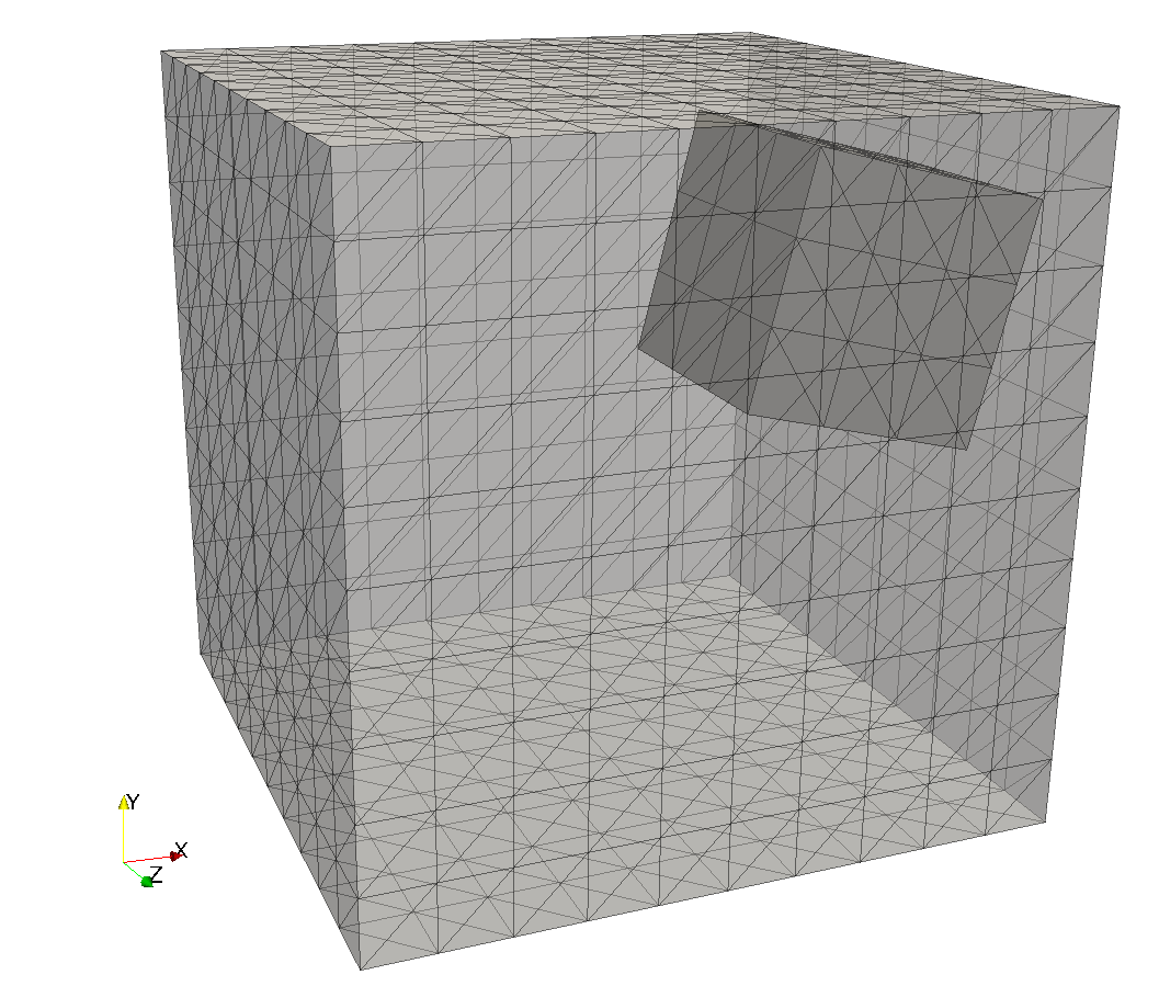
Fig. 9: Mesh configuration for the Poisson problem.

The Nitsche approximation was computed on a sequence of meshes with decreasing mesh size $h_{\mathrm{max}}=1/N$ for the tessellations $\mathcal{T}_{0}$ and $\mathcal{T}_{2}$, starting at $N=14$ and stopping at $N=104$. For the integration over cut cells and interface facets, barycenter quadrature was employed. The resulting linear systems were solved by the preconditioned conjugate gradient method as implemented in PETSc in combination with the algebraic multigrid solver from Hypre used as a preconditioner. For both the standard finite element method and the overlapping mesh method, a mesh independent number of CG iterations was observed (3–4 and 9-11, respectively). All computations were carried out on a Macbook Pro equipped with a $2.66$ GHz Intel Core i7 processor and $8$ GB of RAM (1066 MHz DDR3). The benchmarks were repeated 10 times and averaged to obtain the reported results.

Convergence

As the theoretical results recalled in (11)–(12) predict, an optimal convergence rate in both in the $H^{1}$- and $L^{2}$-norm is observed; see Figure 11. Figure 10 clearly illustrates the smooth transition from the solution part $u_{1}$ defined on the overlapped mesh $\mathcal{T}_{1}$ to the part $u_{2}$ defined on the overlapping mesh $\mathcal{T}_{2}$.

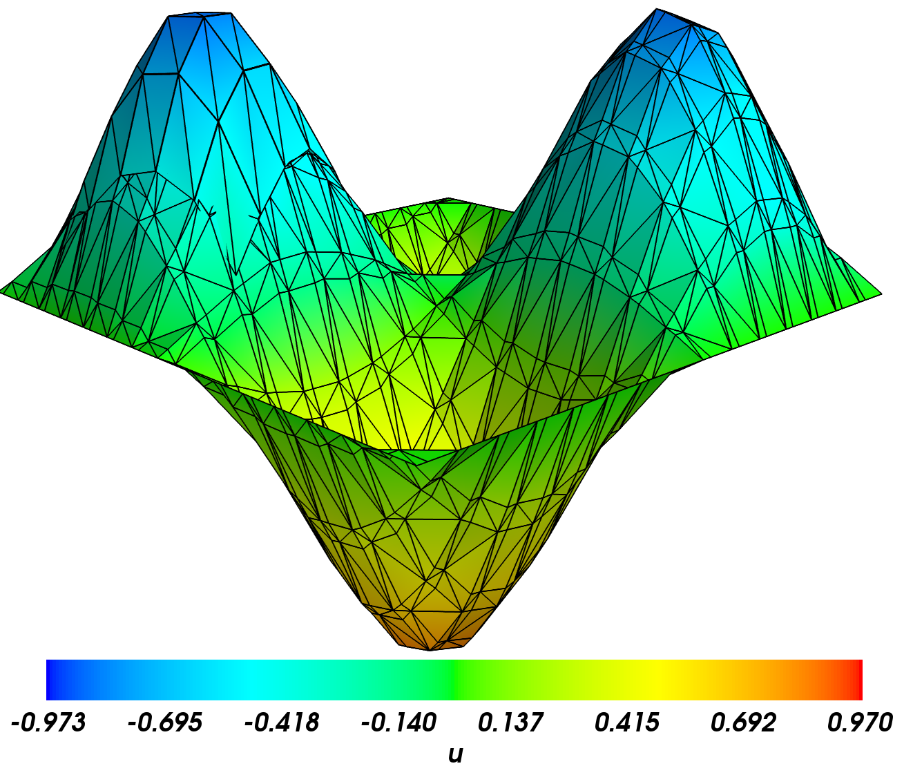
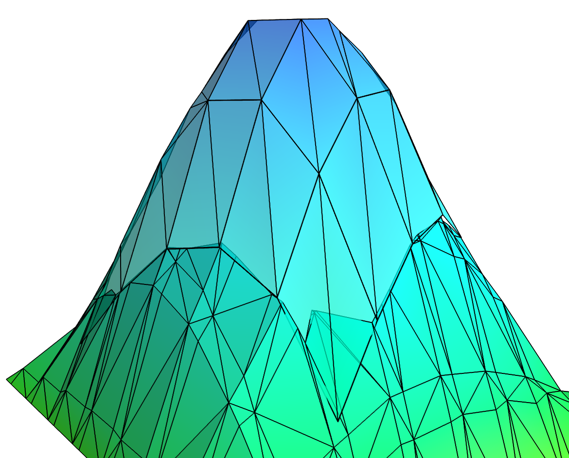
Fig. 10: Two-dimensional cross-section of the three-dimensional solution of the Poisson problem showing good agreement between solutions computed on the overlapped and the overlapping mesh. (Left) Both solution parts patched together. The solution on the overlapping mesh can be seen far to the left. (Right) A zoom revealing the small discontinuity between solutions at the common interface.

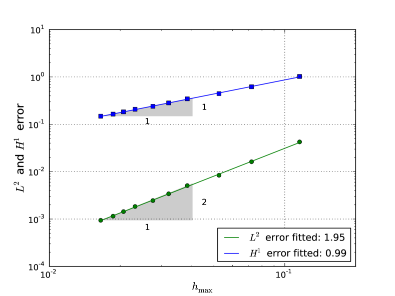
Fig. 11: Convergence of the Nitsche approximation in the $L^{2}$- and $H^{1}$-norm for the Poisson problem.

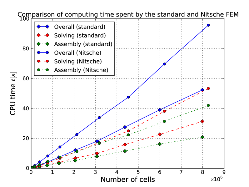
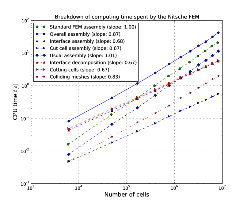
Fig. 12: (Top) Overall computing time spent by the standard FEM and the Nitsche FEM. (Bottom) Breakdown of the assembly time spent by the Nitsche method compared to the overall assembly time for the standard FEM. Note the expected slope of 1 for the standard (usual) assembly and of $2/3$ for the interface related operations. The graph shows that, asymptotically, overall assembly time will be dominated by standard assembly.

Benchmarks

The comparison in Figure 12 shows that the Nitsche overlapping mesh method is only twice as expensive as the standard finite element method for the same mesh size and approximately the same number of degrees of freedom. A breakdown of the computing time shows that both the assembly and the solution of the linear system become twice as expensive when the overlapping mesh method is used. The latter can be attributed to the observed higher iteration numbers. The CPU time for the linear solve displays a kink in the slope at ca 3 and 4.5 million cells for the standard and Nitsche FEM, respectively, which may be attributed to the problem size increasing beyond a hardware-specific threshold (cache or memory size) that induces overhead.

A further breakdown of the assembly time is shown at the bottom of Figure 12. We note that while the number of cells scales like $\mathcal{O}(h^{-3})$ on a regular grid, the number of facets scales like $O(h^{-2})$. Consequently, all purely interface related operations with linear complexity should scale like $N^{2/3}$, where $N$ is the number of cells. This is also the case for the interface decomposition, computation of the cut cells, and integration over the interface and the cut cells. On the other hand, the initial collision detection between the overlapped and the overlapping mesh is somewhat more expensive as it involves the searching of tree-like data structures (adding a logarithmic factor to the complexity). However, this extra cost is negligible compared to the total computing time. In conclusion, the timings depicted in Figure 12 indicate that the cost of assembly for the Nitsche overlapping mesh method is comparable to standard finite element assembly, and its relative efficiency increases with increasing mesh size.

A note on ill-conditioned stiffness matrices

As analyzed in Burman [19] and illustrated by numerical experiments in [47], the stiffness matrix stemming from Nitsche’s method on overlapping meshes and related schemes can be ill-conditioned if the intersection gives very small elements, compared to the original element size. Different approaches have been investigated to cure the schemes from ill-conditioned systems, either by choosing proper weights for the interface [38], replacing basis functions on small elements by extensions of basis functions on larger neighboring elements, or through the use of a so-called ghost-penalty [19, 20]. For the current work, the only precaution was to skip all cut cells with a relative measure of size smaller that $10^{-15}$. In our numerical experiments, we observed a mesh-independent iteration number which indicates that ill-conditioning was not present. However, proper handling of small cells by introducing ghost penalties has been studied recently for the Stokes problem in Massing et al. [48].

5.2 Linear elasticity

As a second example, we consider a linear elastic body occupying a domain $\Omega_{0}$ in $\mathbb{R}^{3}$ consisting of two subdomains $\Omega_{1}$ and $\Omega_{2}$ with possibly different material parameters. The displacement and the stresses are assumed to be continuous across the interface $\Gamma=\partial\Omega_{1}\cap\partial\Omega_{2}$ between the subdomains. The corresponding linear elasticity problem then takes the form: find the displacement $\mathbf{u}:\Omega_{0}\rightarrow\mathbb{R}^{3}$ such that

$$-\operatorname{div}({\boldsymbol{\sigma}}(\mathbf{u}_{i})) =\mathbf{f}_{i} \text{in }\Omega_{i},\quad i=1,2,$$ (27)

$$[{\boldsymbol{\sigma}}(\mathbf{u})\cdot\mathbf{n}] =\mathbf{0} \text{on }\Gamma,$$ (28)

$$[\mathbf{u}] =\mathbf{0} \text{on }\Gamma,$$ (29)

$$\mathbf{u} =\mathbf{0} \text{on }\partial\Omega_{0,\mathrm{D}}{},$$ (30)

$${\boldsymbol{\sigma}}(\mathbf{u})\cdot\mathbf{n} =\mathbf{g} \text{on }\partial\Omega_{0,\mathrm{N}}{}.$$ (31)

Here, the stress tensor ${\boldsymbol{\sigma}}$ is related to the displacement vector $\mathbf{u}$ by Hooke’s law

$${\boldsymbol{\sigma}}(\mathbf{u}_{i})=2\mu_{i}{\boldsymbol{\epsilon}}(\mathbf{u}_{i})+\lambda_{i}\text{tr}({\boldsymbol{\epsilon}}(\mathbf{u}_{i}))\mathbf{I}\quad\text{in }\Omega_{i},\quad i=1,2,$$ (32)

where $\lambda_{i}$ and $\mu_{i}$ are the Lamé parameters in $\Omega_{i}$ for $i=1,2$ and ${\boldsymbol{\epsilon}}(\mathbf{v})=(\operatorname{grad}(\mathbf{v})+\operatorname{grad}(\mathbf{v})^{\top})/{2}$ is the strain tensor.

Nitsche’s method for the Poisson equation (1) proposed by Hansbo et al. [33] can be adapted to the case of the linear elastic problem (27)–(31) and takes the following form: find $\mathbf{u}_{h}\in\mathbf{W}_{h}$ such that

$$a(\mathbf{u}_{h},\mathbf{v})=l(\mathbf{v})\quad\forall\,\mathbf{v}\in\mathbf{W}_{h},$$ (33)

where

$$a(u,v) =\sum_{i=1}^{2}\int_{\Omega_{i}}{\boldsymbol{\sigma}}(\mathbf{u}_{i}):\operatorname{grad}(\mathbf{v}_{i})\,\mathrm{d}x$$ (34)

$$\qquad-\underbrace{\int_{\Gamma}{\boldsymbol{\sigma}}(\mathbf{u}_{1})\cdot\mathbf{n}\,[\mathbf{v}]}_{\text{Stress balance}}\,\mathrm{d}S-\underbrace{\int_{\Gamma}{\boldsymbol{\sigma}}(\mathbf{v}_{1})\cdot\mathbf{n}\,[\mathbf{u}]}_{\text{Symmetrization}}\,\mathrm{d}S+\underbrace{\gamma\int_{\Gamma}h^{-1}[\mathbf{u}]\cdot[\mathbf{v}]}_{\text{Penalty/Stabilization}}\,\mathrm{d}S,$$ (35)

$$l(v) =\int_{\Omega}\mathbf{f}\cdot\mathbf{v}\,\mathrm{d}x+\int_{\partial\Omega}\mathbf{g}\cdot\mathbf{v}\,\mathrm{d}s,$$ (36)

with $\gamma$ a positive penalty parameter. Assuming that the elastic material is not nearly incompressible ($\lambda$ remains bounded), we may extend the analysis in Hansbo et al. [33] and prove optimal order a priori error estimates. See Hansbo and Larson [35] and Becker et al. [14] for details on discontinuous Galerkin methods for elasticity problems.

Test configuration and numerical results

We consider the linear elasticity problem (27)–(31) with $\Omega_{0}=(-2,2)^{3}\subset\mathbb{R}^{3}$ which is overlapped by a propeller-like domain $\Omega_{1}=(-1,1)\times P$ where $P=(-1,1)\times(-0.2,0.2)\cup(-0.2,0.2)\times(-1,1)\subset\mathbb{R}^{2}$; see Figure 3. The right-hand side is zero and the boundary conditions on $\partial\Omega_{0}$ are defined by

$$\begin{cases}\mathbf{u}=0,&\quad\text{on }(-2,2)^{2}\times\{-2\},\\ {\boldsymbol{\sigma}}(\mathbf{u})\cdot\mathbf{n}=0,&\quad\text{on }\partial((-2,2)^{2})\times(-2,2),\\ {\boldsymbol{\sigma}}(\mathbf{u})\cdot\mathbf{n}=\mathbf{g}&\quad\text{on }(-2,2)^{2}\times\{2\},\end{cases}$$ (37)

where $\mathbf{g}$ represents a combination of pure tangential, rotational force and a normal pressure:

$$\mathbf{g}(x,y,z)=\dfrac{(-y,x,0)^{\top}}{5\sqrt{x^{2}+y^{2}}}-(0,0,2-\sqrt{x^{2}+y^{2}})^{\top}.$$ (38)

The Lamé parameters are given by $\mu_{i}=E_{i}/(2+2\nu_{i}),\lambda_{i}=E_{i}\cdot\nu_{i}/((1+\nu_{i})(1-2\nu_{i}))$ in $\Omega_{i}$ for $i=1,2,$ with $E_{1}=10$, $E_{2}=0.1\cdot E_{1}$, $\nu_{1}=\nu_{2}=0.3$.

The numerical results are shown in Figures 13 and 14. The results indicate a “smooth” transition of the solution from the overlapped mesh to the overlapping mesh.

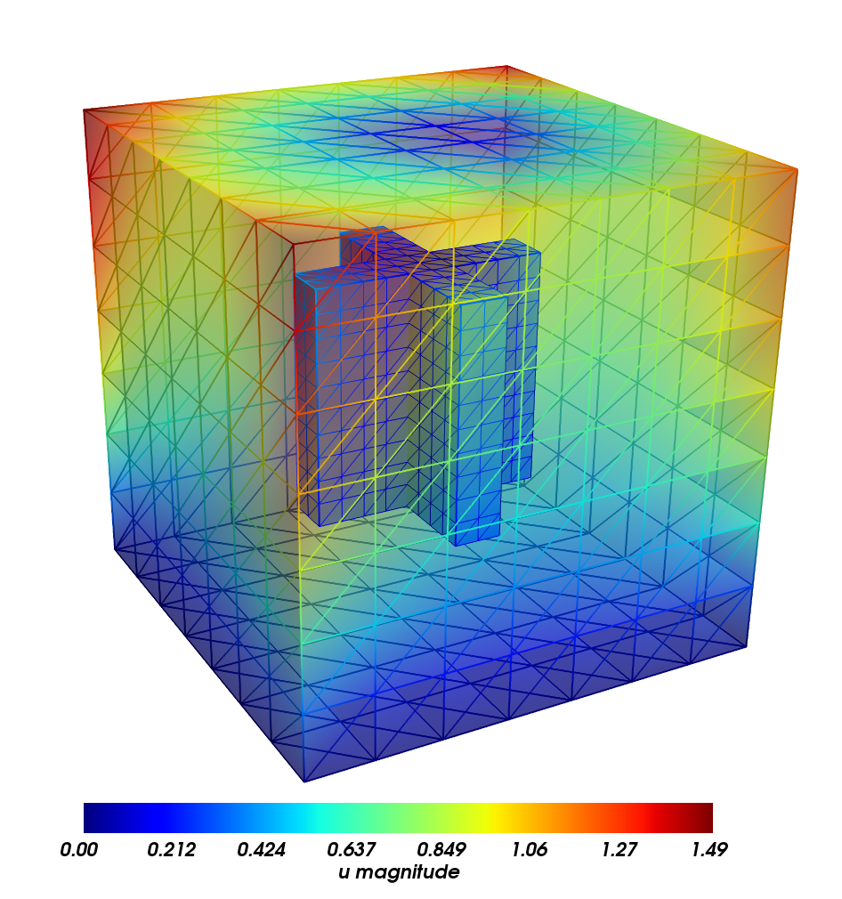
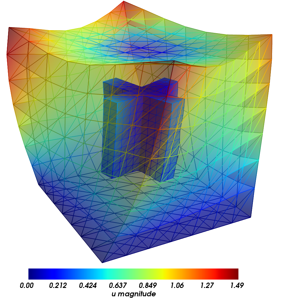
Fig. 13: (Left) Undeformed, original domain consisting of a cube overlapped by a propeller-like domain. (Right) The deformed domain. The color bar corresponds to the norm of the displacement $\mathbf{u}$.

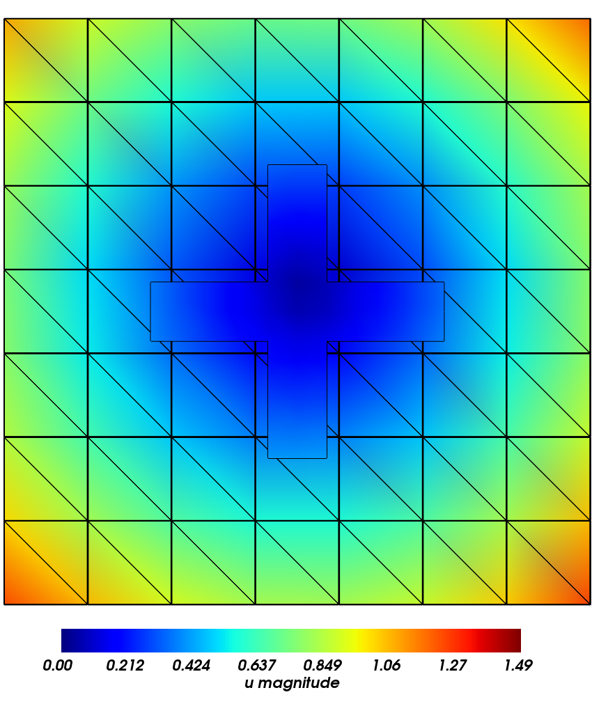
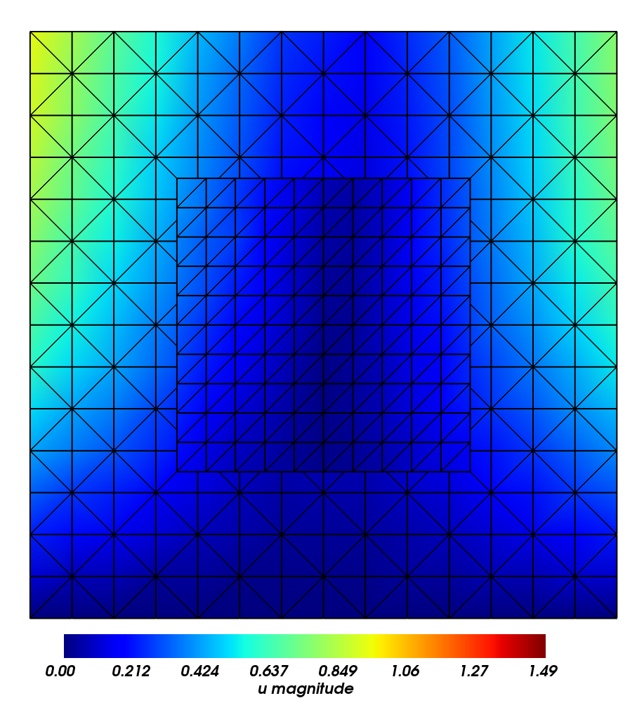
Fig. 14: (Left) Magnitude of the displacement $\mathbf{u}$ in a cross-section through the $xy$-plane of the solution from Figure 13. (Right) Magnitude of the displacement $\mathbf{u}$ in the cross-section through the $xz$-plane. Despite a very coarse resolution, both figures show a “smooth” transition of the solution from the domain $\Omega_{1}$ to $\Omega_{2}$.

6 Conclusions and outlook

We have demonstrated that overlapping mesh methods, in particular the Nitsche overlapping mesh method, may be implemented efficiently in three space dimensions through the use of tree search data structures and tools from computational geometry. Numerical tests show that optimal order convergence is obtained, that the overhead of the overlapping mesh method compared to a standard finite element method is small (roughly factor two), and that the overhead is decreasing as the size of the mesh is increased.

In the future, we plan to extend our implementation and the techniques studied in this work to handle fluid–structure interaction problems as well as contact problems. Furthermore, we plan to fully automate the implementation of Nitsche formulations on overlapping meshes by adding code generation capabilities for interface terms to FEniCS.

References

- [1] Cgal, Computational Geometry Algorithms Library, software package. URL http://www.cgal.org.
- [2] gts, GNU Triangulated Surface Library, software package. URL http://gts.sourceforge.net/.
- Akenine-Möller et al. [2008] T. Akenine-Möller, E. Haines, and N. Hoffman. Real-time rendering. A.K. Peters Ltd, 2008.
- Alnæs [2012] Martin S. Alnæs. UFL: a Finite Element Form Language, chapter 17. Springer, 2012.
- Alnæs et al. [2009] Martin S. Alnæs, Anders Logg, Kent-Andre Mardal, Ola Skavhaug, and Hans Petter Langtangen. Unified framework for finite element assembly. Int. J. Comput. Sci. Eng., 4(4):231–244, 2009.
- Areias and Belytschko [2006] P. Areias and T. Belytschko. A comment on the article “A finite element method for simulation of strong and weak discontinuities in solid mechanics” by A. Hansbo and P. Hansbo. Commentary. Comput. Methods Appl. Mech. Engrg., 195(9-12):1275–1276, 2006.
- Baiges and Codina [2009] J. Baiges and R. Codina. The fixed-mesh ALE approach applied to solid mechanics and fluid-structure interaction problems. International Journal for Numerical Methods in Engineering, 81:1529–1557, 2009.
- Balay et al. [1997] Satish Balay, William D. Gropp, Lois Curfman McInnes, and Barry F. Smith. Efficient management of parallelism in object oriented numerical software libraries. In E. Arge, A. M. Bruaset, and H. P. Langtangen, editors, Modern Software Tools in Scientific Computing, pages 163–202. Birkhäuser Press, 1997.
- Balay et al. [2010] Satish Balay, Jed Brown, Kris Buschelman, Victor Eijkhout, William D. Gropp, Dinesh Kaushik, Matthew G. Knepley, Lois Curfman McInnes, Barry F. Smith, and Hong Zhang. PETSc users manual. Technical Report ANL-95/11 - Revision 3.1, Argonne National Laboratory, 2010.
- Balay et al. [2011] Satish Balay, Jed Brown, Kris Buschelman, William D. Gropp, Dinesh Kaushik, Matthew G. Knepley, Lois Curfman McInnes, Barry F. Smith, and Hong Zhang. PETSc Web page, 2011. URL http://www.mcs.anl.gov/petsc.
- Bastian et al. [2004] P. Bastian, M. Droske, C. Engwer, R. Klöfkorn, T. Neubauer, M. Ohlberger, and M. Rumpf. Towards a unified framework for scientific computing. In Proc. of the 15th International Conference on Domain Decomposition Method, 2004.
- Bastian et al. [2010a] P. Bastian, F. Heimann, and S. Marnach. Generic implementation of finite element methods in the Distributed and Unified Numerics Environment (DUNE). Kybernetika, 46(2):294–315, 2010a.
- Bastian et al. [2010b] Peter Bastian, Gerrit Buse, and Oliver Sander. Infrastructure for the coupling of Dune grids. Numerical Mathematics and Advanced Applications 2009, pages 107–114, 2010b.
- Becker et al. [2009] Roland Becker, Erik Burman, and Peter Hansbo. A Nitsche extended finite element method for incompressible elasticity with discontinuous modulus of elasticity. Comput. Methods Appl. Mech. Engrg., 198(41-44):3352–3360, 2009.
- Belytschko et al. [2001] Ted Belytschko, Nicolas Moës, S. Usui, and C. Parimi. Arbitrary discontinuities in finite elements. International Journal for Numerical Methods in Engineering, 50(4):993–1013, 2001.
- Berti [2002] Guntram Berti. Generic programming for mesh algorithms: Towards universally usable geometric components. In Proceedings of the Fifth World Congress on Computational Mechanics,Vienna University of Technology July, 2002.
- Berti [2006] Guntram Berti. GrAL - The Grid Algorithms Library. Future Generation Computer Systems, 22, 2006.
- Botsch et al. [2002] M. Botsch, S. Steinberg, S. Bischoff, and L. Kobbelt. OpenMesh - a generic and efficient polygon mesh data structure, 2002.
- Burman [2010] E. Burman. Ghost penalty. Comptes Rendus Mathematique, 348(21-22):1217–1220, 2010.
- Burman and Hansbo [2012] E. Burman and P. Hansbo. Fictitious domain finite element methods using cut elements: II. A stabilized Nitsche method. Appl. Numer. Math., 62(4), 2012.
- Chazelle and Palios [1990] Bernard Chazelle and Leonidas Palios. Triangulating a non-convex polytope. Discrete & Computational Geometry, 5(1):505–526, 1990.
- Chesshire and Henshaw [1990] G. Chesshire and W. D. Henshaw. Composite overlapping meshes for the solution of partial differential equations. Journal of Computational Physics, 90(1):1–64, 1990.
- Cools [1997] Ronald Cools. Constructing cubature formulae: the science behind the art. Acta Numerica, 6(-1):1–54, January 1997.
- Daux et al. [2000] Christophe Daux, Nicolas Mo s, John Dolbow, Natarajan Sukumar, and Ted Belytschko. Arbitrary branched and intersecting cracks with the extended finite element method. International Journal for Numerical Methods in Engineering, 48(12):1741–1760, 2000.
- Day and Bochev [2008] D. Day and P. Bochev. Analysis and computation of a least-squares method for consistent mesh tying. J. Comput. Appl. Math., 218(1):21–33, August 2008.
- Dhia and Guillaume Rateau [2005] Hashmi Ben Dhia and Guillaume Rateau. The Arlequin method as a flexible engineering design tool. International Journal for Numerical Methods in Engineering, 62(11):1442–1462, 2005.
- Ericson [2005] C. Ericson. Real-time collision detection. Morgan Kaufmann, 2005.
- Fournier and Montuno [1984] A. Fournier and D. Y. Montuno. Triangulating Simple Polygons and Equivalent Problems. ACM Transactions on Graphics, 3(2):153–174, 1984.
- Fries [2008] T. P. Fries. A corrected XFEM approximation without problems in blending elements. International Journal for Numerical Methods in Engineering, 75(5):503–532, 2008.
- Fries [2009] T. P. Fries. The intrinsic XFEM for two-fluid flows. International Journal for Numerical Methods in Fluids, 60(4):437–471, 2009.
- Fries and Belytschko [2010] T. P. Fries and T. Belytschko. The extended/generalized finite element method: An overview of the method and its applications. International Journal for Numerical Methods in Engineering, 84(April):253–304, 2010.
- Hansbo and Hansbo [2002] A. Hansbo and P. Hansbo. An unfitted finite element method, based on Nitsche’s method, for elliptic interface problems. Comput. Methods Appl. Mech. Engrg., 191(47-48):5537–5552, 2002.
- Hansbo et al. [2003] A. Hansbo, P. Hansbo, and Mats G. Larson. A Finite Element Method on Composite Grids based on Nitsche’s Method. ESAIM, Math. Model. Num. Anal., 37(3):495–514, 2003.
- Hansbo and Hansbo [2004] Anita Hansbo and Peter Hansbo. A finite element method for the simulation of strong and weak discontinuities in solid mechanics. Comput. Methods Appl. Mech. Engrg., 193(33-35):3523–3540, 2004.
- Hansbo and Larson [2002] P. Hansbo and M. G. Larson. Discontinuous Galerkin methods for incompressible and nearly incompressible elasticity by Nitsche’s method. Comput. Methods Appl. Mech. Engrg., 191(17–18):1895–1908, 2002.
- Heroux et al. [2005] Michael A. Heroux, Roscoe A. Bartlett, Vicki E. Howle, Robert J. Hoekstra, Jonathan J. Hu, Tamara G. Kolda, Richard B. Lehoucq, Kevin R. Long, Roger P. Pawlowski, Eric T. Phipps, Andrew G. Salinger, Heidi K. Thornquist, Ray S. Tuminaro, James M. Willenbring, Alan Williams, and Kendall S. Stanley. An overview of the trilinos project. ACM Trans. Math. Softw., 31(3):397–423, 2005.
- Jirásek and Belytschko [2002] M. Jirásek and T. Belytschko. Computational resolution of strong discontinuities. In Fifth world congress on computational mechanics, pages 7–12, 2002.
- Johansson and Larson [2012] August Johansson and Mats G. Larson. A high order discontinuous Galerkin Nitsche method for elliptic problems with fictitious boundary. submitted to Numerische Mathematik, 2012.
- Kirby and Logg [2006] Robert C. Kirby and Anders Logg. A Compiler for Variational Forms. ACM Trans. Math. Softw., 32(3):417–444, 2006.
- Lee and Requicha [1982] Y. T. Lee and A. A. G. Requicha. Algorithms for computing the volume and other integral properties of solids. I. known methods and open issues. Communications of the ACM, 25(9):635–641, 1982.
- Logg [2007] Anders Logg. Automating the finite element method. Arch. Comput. Methods Eng., 14(2):93–138, 2007.
- Logg [2009] Anders Logg. Efficient representation of computational meshes. Int. J. of Computat. Sci. Eng., 4(4):283–295, 2009.
- Logg and Wells [2010] Anders Logg and Garth N. Wells. DOLFIN: Automated finite element computing. ACM Trans. Math. Softw., 37(2), 2010.
- Logg et al. [2012a] Anders Logg, Kent-Andre Mardal, Garth N. Wells, et al. Automated Solution of Differential Equations by the Finite Element Method. Springer, 2012a.
- Logg et al. [2012b] Anders Logg, Kristian B. Ølgaard, Marie E. Rognes, and Garth N. Wells. FFC: the FEniCS Form Compiler, chapter 11. Springer, 2012b.
- Logg et al. [2012c] Anders Logg, Garth N. Wells, and Johan Hake. DOLFIN: a C++/Python finite element library, chapter 10. Springer, 2012c.
- Massing [2012] A. Massing. Analysis and implementation of finite element methods on overlapping and fictitious domains. PhD thesis, University of Oslo, 2012.
- Massing et al. [2012] A. Massing, Mats G. Larson, A. Logg, and Marie E. Rognes. A stabilized Nitsche overlapping mesh method for the Stokes problem. submitted, 2012.
- Mayer et al. [2009] U. M. Mayer, A. Gerstenberger, and W. A. Wall. Interface handling for three-dimensional higher-order XFEM-computations in fluid-structure interaction. International Journal for Numerical Methods in Engineering, 79(7):846–869, 2009.
- Mayer et al. [2010] U. M. Mayer, A. Popp, A. Gerstenberger, and W. A. Wall. 3D fluid–structure-contact interaction based on a combined XFEM FSI and dual mortar contact approach. Comput. Mech., 46(1):53–67, 2010.
- Mirtich [1996] Brian Mirtich. Fast and accurate computation of polyhedral mass properties. journal of graphics tools, 1(2):31–50, 1996.
- Moës et al. [1999] N. Moës, J. Dolbow, and T. Belytschko. A finite element method for crack growth without remeshing. Int. J. Numer. Meth. Engng, 46:131–150, 1999.
- Natarajan et al. [2009] S. Natarajan, S. Bordas, and D. R. Mahapatra. Numerical integration over arbitrary polygonal domains based on Schwarz-Christoffel conformal mapping. International Journal for Numerical Methods in Engineering, 80(1):103–134, 2009.
- Natarajan et al. [2010] Sundararajan Natarajan, D. Roy Mahapatra, and Stéphane P. A. Bordas. Integrating strong and weak discontinuities without integration subcells and example applications in an XFEM/GFEM framework. International Journal for Numerical Methods in Engineering, pages 269–294, July 2010.
- Ølgaard et al. [2008] Kristian B. Ølgaard, Anders Logg, and Garth N. Wells. Automated code generation for discontinuous galerkin methods. SIAM Journal on Scientific Computing, 31(2):849–864, 2008.
- Ruppert and Seidel [1989] J. Ruppert and R. Seidel. On the difficulty of tetrahedralizing 3-dimensional non-convex polyhedra. In Proceedings of the fifth annual symposium on Computational geometry - SCG ’89, pages 380–392, New York, New York, USA, June 1989. ACM Press.
- Schneider and Eberly [2003] Philip J. Schneider and David H. Eberly. Geometric tools for computer graphics. Morgan Kaufmann, 2003.
- Sukumar et al. [2000] N. Sukumar, N. Moës, B. Moran, and T. Belytschko. Extended finite element method for three-dimensional crack modelling. International Journal for Numerical Methods in Engineering, 48(11):1549–1570, 2000.
- Yang and Laursen [2008] B. Yang and T. A. Laursen. A contact searching algorithm including bounding volume trees applied to finite sliding mortar formulations. Comput. Mech., 41(2):189–205, 2008.
- Yu [2005] Z. Yu. A DLM/FD method for fluid/flexible-body interactions. Journal of Computational Physics, 207(1):1–27, 2005.
- Zhang et al. [2004] L. Zhang, A. Gerstenberger, X. Wang, and W. K. Liu. Immersed finite element method. Comput. Methods Appl. Mech. Engrg., 193(21-22):2051–2067, 2004.