Theory of the conductance of interacting quantum wires with good contacts and applications to carbon nanotubes

Abstract

Using bosonization we derive the dc conductance $G(L,T)$ of an interacting quantum wire with good contacts including current relaxing backscattering and Umklapp processes. Our result yields the dependence of the conductance on length $L$ and temperature $T$ in the energy range where the Luttinger model is applicable. For a system where only a part of the current is protected by a conservation law we surprisingly find an unreduced ideal quantum conductance as for a fully ballistic wire. As a second application, we calculate the conductance of metallic single-wall carbon nanotubes in an energy range where backscattering due to phonons dominates. In contrast to previous studies we treat the electrons as interacting by using the Luttinger liquid formulation. The obtained results for the scaling of the dc conductance with temperature and length are compared with experimental data and yield a better description than the previously used non-interacting theory. Possible reasons for the remaining discrepancies in the temperature dependence between theory and experiment are discussed.

I Introduction

In a one-dimensional quantum system the quantization of the transverse momentum means that only a small number of modes are available for transmission. As a consequence, even a fully ballistic quantum wire with adiabatic contacts shows a finite quantum conductance,Landauer (1957) $G=2ne^{2}/h$, where $n$ is the number of modes and the factor of $2$ arises due to spin degeneracy. If momentum relaxation by Umklapp or backscattering can be neglected then a wire with electron-electron interactions can be described as a Luttinger liquid. In this case a renormalization of the conductance to $G=2nKe^{2}/h$ with a Luttinger parameter $K<1$ for repulsive interactions might be expected.Kane and Fisher (1992); Ogata and Fukuyama (1994) However, such a renormalization was never observed experimentallyTarucha et al. (1995) and does not take into account the contacts. Assuming that the contacts are adiabatic it has been shown that the conductance remains unrenormalized by the electron-electron interactions within the wire.Maslov and Stone (1995); Safi and Schulz (1995) In any realistic system the conductance will, however, be affected by backscattering processes caused, for example, by phonons or impurities in the bulk of the wire.Kane and Fisher (1992); Kane et al. (1998); Ristivojevic and Nattermann (2008) In addition, backscattering processes at the junctions between the wire and the leads can also renormalize the conductance.Furusaki and Nagaosa (1996); Ogata and Fukuyama (1994); Sedlmayr et al. (2012) Both contributions can be described at low energies by adding interactions to the Luttinger liquid Hamiltonian and lead, in general, to a temperature- and length-dependent conductance.

Experimentally, two types of systems have mainly been used to study electronic transport in quantum wires. In semiconductor heterostructures, wide two-dimensional electron gases are formed which are subsequently laterally confined by applying gate voltages. This approach makes it possible to obtain very clean wires which show clear signatures of conductance quantization.Tarucha et al. (1995) The other important experimental system are carbon nanotubes (CNTs).Charlier et al. (2007) Single-wall carbon nanotubes can either be semi-conducting or metallic depending on their wrapping vector. The basic electronic properties of CNTs can be understood by viewing them as rolled-up graphene sheets.Kane et al. (1997); Egger and Gogolin (1997) The momentum transverse to the tube direction is quantized leading to a finite number of bands. For a metallic tube two of these bands cross at the two Fermi points so that in the low-energy limit we are left with a system consisting of two left- and two right-moving fermionic modes. Including spin degeneracy the quantum conductance of a ballistic CNT would therefore be $G_{0}=4e^{2}/h$. In a first important experiment,Bockrath et al. (1997) ropes of single-wall carbon nanotubes on Si/SiO₂ substrates were studied. In this system charging effects and resonant tunneling were observed. The conductance was found to be small and transport dominated by the probability to tunnel an electron between the contact and the CNT. For a Luttinger liquid with $n=2$ bands such as a CNT, the temperature-dependence of the tunnel conductance is well-known and scales as $T^{\alpha}$ with $\alpha=(K_{c+}+K_{c+}^{-1}-2)/8$ for tunneling into the bulk of the wire and $\alpha=(K_{c+}^{-1}-1)/4$ for tunneling at an end of the wire.Egger and Gogolin (1997) Experimental dataBockrath et al. (1997, 1999); Yao et al. (1999) for tunneling into the bulk or an end of a CNT were consistent with these two formulas with a single Luttinger parameter $K_{c+}\approx 0.2-0.4$ for the total charge mode as expected by theory.Egger and Gogolin (1997); Yoshioka and Odintsov (1999) Spin-lattice relaxation rates $1/T_{1}$ have also been interpreted in terms of a Luttinger liquid with $K_{c+}\approx 0.2$.Singer et al. (2005); Dóra et al. (2007)

In recent years, single CNTs have been successfully contacted as well. In one such experiment,Purewal et al. (2007) almost perfect contacts have been realized so that the conductance of short wires at low temperatures was close to the ideal quantum conductance $G_{0}$. Contacting the same CNT at various distances Purewal et al.Purewal et al. (2007) were further able to measure the conductance not only as a function of temperature but also as a function of length. In contrast to the earlier experiment by Bockrath et al.Bockrath et al. (1997) the good contacts imply that the conductance is no longer dominated by tunneling processes but rather by electron backscattering in the bulk of the wire. Backscattering can be caused by impurities which are often relevant perturbations and can completely suppress the conductance below a temperature scale $T_{K}$.Kane and Fisher (1992) At temperatures $T\gg T_{K}$, on the other hand, irrelevant backscattering due to phonons is expected to be the dominant contribution in clean samples. Treating the electrons in the CNT as non-interacting it has been shown that acoustic phonon modes give rise to a resistivity which increases linearly with temperature.Kane et al. (1998); Park et al. (2004); Ilani and McEuen (2010) At half-filling purely electronic Umklapp scattering also has to be taken into account and induces a charge gap $\Delta_{c}$. The conductance for $T<\Delta_{c}$ then shows thermally activated behavior. For $T\gg\Delta_{c}$, on the other hand, Umklapp scattering can be treated perturbatively and leads to a resistivity which—similarly to the phonon contribution—increases linearly with temperature if the electrons are assumed to be noninteracting.Balents and Fisher (1997) However, while the phonon contribution is proportional to $1/R_{a}$, where $R_{a}$ is the tube radius, the Umklapp contribution scales as $1/R_{a}^{2}$ and can therefore be neglected except for very narrow tubes.

In this paper we will consider electronic transport in a quantum wire described by the generic low-energy HamiltonianGiamarchi (2004)

$$H=-\text{i}v_{F}\sum_{r,\alpha,\sigma}r\int dx\,\Psi^{\dagger}_{r\alpha\sigma}(x)\partial_{x}\Psi_{r\alpha\sigma}(x)\,.$$ (1)

Here $v_{F}$ is the Fermi velocity and $\Psi^{(\dagger)}_{r\alpha\sigma}$ a fermionic annihilation (creation) operator with $\sigma=\pm$ being the spin, and $\alpha=1,\cdots,n$ a band index. The fermionic field in the low-energy limit is split into right movers $\Psi_{+,\alpha\sigma}\equiv\Psi_{R,\alpha\sigma}$ and left movers $\Psi_{-,\alpha\sigma}\equiv\Psi_{L,\alpha\sigma}$. We will then use standard Abelian bosonization to express the fermionic operators in terms of bosonic fields

$$\Psi_{r\alpha\sigma}(x)=\frac{\eta_{r\alpha\sigma}}{\sqrt{2\pi\bar{a}}}\text{e}^{i[k_{F}(r,\alpha)x+r\sqrt{2\pi}\phi_{r\alpha\sigma}(x)]}.$$ (2)

Here $\eta_{r\alpha\sigma}$ are Klein factors ensuring the fermionic commutation rules and $\bar{a}$ is a cutoff of the order of the lattice constant $a$. The Fermi momentum $k_{F}(r,\alpha)$ associated with each of the modes depends on the band structure of the microscopic model. We further assume that we can represent the Hamiltonian (1) using (2) by

$$H=\frac{1}{2}\sum_{j,\delta}\int dx\left\{v_{j\delta}K_{j\delta}(\partial_{x}\theta_{j\delta})^{2}+\frac{v_{j\delta}}{K_{j\delta}}(\partial_{x}\phi_{j\delta})^{2}\right\}$$ (3)

where the new fields fulfill the commutation relation $[\theta_{j\delta}(x),\phi_{j^{\prime}\delta^{\prime}}(x^{\prime})]=-\frac{i}{2}\delta_{jj^{\prime}}\delta_{\delta\delta^{\prime}}\mbox{sgn}(x-x^{\prime})$. The indices $j$, $\delta$ are now indices of the diagonal modes obtained by combining the bosonic fields $\phi_{r\alpha\sigma}$ in an appropriate way. The Hamiltonian (3) includes the density-density type electron-electron interactions which lead to a renormalization of the velocity $v_{F}\to v_{j\delta}$ and introduce the Luttinger parameters $K_{j\delta}$.

The charge density can be expressed as $\rho=e\sqrt{\frac{2n}{\pi}}\partial_{x}\phi_{\bar{j}\bar{\delta}}$ through one of the bosonic fields which we denote by $\phi_{\bar{j}\bar{\delta}}$. The current density $j(x)$ is then obtained by the continuity equation

$$\partial_{t}\rho(x)=-i[\rho(x),H]=-\partial_{x}j(x)$$ (4)

leading to

$$j=-e\sqrt{\frac{2n}{\pi}}\partial_{t}\phi_{\bar{j}\bar{\delta}}\,.$$ (5)

In the following we will use the short hand notation $\phi\equiv\phi_{\bar{j}\bar{\delta}}$ for the mode related to the electric charge and current density.

Our paper is organized as follows: In Sec. II we generalize the approach by Maslov and StoneMaslov and Stone (1995) to derive a formula for the dc conductance of a quantum wire with good contacts and some form of damping in the bulk of the wire. In Sec. III we then use a self-energy approach to consider damping by Umklapp scattering. In particular, we consider the case of the integrable $XXZ$ model where only part of the current can decay by Umklapp scattering while the rest is protected by a conservation law. Furthermore, we study the general case of damping due to backscattering assisted by other degrees of freedom such as, for example, phonons. For CNTs all microscopic parameters relevant for backscattering by phonons are relatively well-known allowing us to obtain results for the dc conductance which we compare directly to experiment in Sec. IV. In the conclusions, Sec. V, we summarize our main results and discuss possible shortcomings of the obtained formulas for the conductance of CNTs.

II Conductance of a wire with contacts and damping

We are interested here in the conductance of a finite end-contacted quantum wire in the linear response regime with some damping in the bulk of the wire. We assume that we can model the leads as one-dimensional ballistic channels with Luttinger parameter $K_{\ell}=1$. The quantum wire itself, on the other hand, is described by the Hamiltonian (3) with a Luttinger parameter for the total charge channel $K_{\mathrm{w}}$, a velocity $v_{\mathrm{w}}$, and a damping rate $\gamma(T)$. This setup is depicted in Fig. 1.

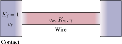
Figure 1: (Color online) Schematic view of the end-contacted quantum wire. The contacts are assumed to be described by a noninteracting channel, $K_{\ell}=1$, with velocity $v_{\ell}$. The quantum wire itself is a Luttinger liquid with the following parameters for the total charge channel: $K_{\mathrm{w}}$ (Luttinger parameter), $v_{\mathrm{w}}$ (velocity), and $\gamma$ (current relaxing damping rate).

The damping in the wire might stem from electron-electron, electron-phonon, or electron-impurity interactions. We will consider the case where the damping is either caused by irrelevant interactions or cases where the interaction is relevant but we are in a temperature regime where the renormalized coupling constant for this interaction is still small so that perturbation theory is applicable. The forward scattering processes in a one-dimensional conductor are marginal and take place on a scattering length of the order of the lattice spacing $a$ leading to new collective excitations described by the Luttinger liquid Hamiltonian with renormalized values for the velocity $v_{\mathrm{w}}$ and the Luttinger parameter $K_{\mathrm{w}}$. We will in the following calculate the conductance in a regime with the backscattering length $\gamma^{-1}(T)\gg a$ so that we can start from the Luttinger liquid description of the wire and include the backscattering processes perturbatively. In addition, we require that $k_{B}T\ll W_{b}$ where $W_{b}$ is the bandwidth so that a linearization of the dispersion near the Fermi points is a valid approximation.

There is also one further approximation which we will use in the following. Strictly speaking one should first calculate the Green’s function for the Luttinger liquid in the contact-wire-contact geometry following the approach by Maslov and Stone.Maslov and Stone (1995) Using this Green’s function one should then perturbatively include the backscattering to obtain the damping in the system. However, as the system is no longer homogeneous it seems an impossible task to solve the resultant Dyson’s equation to sum up a series of diagrams. Instead, we only consider the regime where the coherence length $\xi$ of the considered scattering process is much smaller than the length $L$ of the wire. These coherence lengths are, for example, approximately given by $\xi_{e}\propto\hbar v_{F}/k_{B}T$ and $\xi_{ph}\propto\hbar v_{ph}/k_{B}T$ for the electron, respectively phonon, degrees of freedom. Then we can assume that the majority of the backscattering leading to the damping occurs in the bulk regions and calculate the relaxation rate $\gamma$ by using the electronic Green’s function for an infinite wire. This damping is then already included in our approach when calculating the Green’s function in the contact-wire-contact geometry. We will return to this point in Sec. IV when comparing with experiments on CNTs. To summarize, we make the following assumptions: (1) $k_{B}T\ll W_{b}$ so that a linearization of the spectrum is a valid approximation. (2) The backscattering length $\gamma^{-1}(T)\gg a$ so that we can include forward scattering first and treat backscattering perturbatively. (3) A coherence length of the relevant backscattering process $\xi\ll L$ so that most of the backscattering takes place in the bulk of the wire and can be calculated by using the bulk electronic Green’s function.

Our calculations are based on the Kubo formula which requires the calculation of the retarded current-current correlation function. Using the bosonic representation of the current operator, Eq. (5), the Kubo formula for the conductivity can be written asSirker et al. (2009, 2011)

$$\sigma_{\omega}(x,x^{\prime})=i\omega\frac{4ne^{2}}{h}g_{\omega}(x,x^{\prime}).$$ (6)

Here the retarded correlation function $g_{\omega}(x,x^{\prime})=\langle\phi(x)\phi(x^{\prime})\rangle^{\rm ret}_{\omega}$ can be obtained by an analytical continuation of the Matsubara function $g_{m}(x,x^{\prime})$ at Matsubara frequencies $\omega_{m}=2\pi Tm$.

Let us first consider the case of an infinitely long wire where $g$ depends only on $|x-x^{\prime}|$. In this case the retarded boson propagator can be expressed in Fourier space as

$$\langle\phi\phi\rangle_{\rm ret}(q,\omega)=\frac{v_{\textrm{w}}K_{\textrm{w}}}{\omega^{2}-v_{\textrm{w}}^{2}q^{2}-v_{\textrm{w}}K_{\textrm{w}}\Sigma_{\rm ret}(q,\omega)}\,.$$ (7)

The free propagator is obtained by setting the self-energy $\Sigma_{\rm ret}(q,\omega)=0$. A finite imaginary part of the self-energy, $\Sigma^{\prime\prime}_{\rm ret}(q,\omega)\neq 0$, on the other hand, indicates a finite lifetime of the boson. In writing the boson propagator in this form we have assumed that a Dyson equation is valid. In this case the form of the propagator is generic with the finite lifetime being a consequence of the considered backscattering process.

According to the assumptions explained above, our starting point for calculating the conductance of a quantum wire with contacts at both ends and a damping term in the bulk is the action

$$S=\frac{1}{2\beta}\sum_{\omega_{m}}\int dx\,\!\!\!\!\!\!\! \bigg{\{}\frac{\omega_{m}^{2}}{v_{x}K_{x}}-\frac{\partial}{\partial x}\left(\frac{v_{x}}{K_{x}}\partial_{x}\right)$$ (8)

$$+2\gamma_{x}|\omega_{m}|\bigg{\}}|\phi(x,\omega_{m})|^{2}$$

The position dependent parameters are given by $v_{x}=v_{\mathrm{w}}$, $K_{x}=K_{\mathrm{w}}$ and $\gamma_{x}=\gamma$ in the wire ($0\leq x\leq L$) and by $v_{x}=v_{\ell}$, $K_{x}=K_{\ell}$ and $\gamma_{x}=0$ in the leads ($x<0$ or $x>L$). $\gamma$ in the wire is calculated using the self energy for a homogeneous system.

For an infinite quantum wire the action (8) yields after analytical continuation the boson propagator (7) with

$$\gamma=\frac{1}{2}\operatorname{Im}\frac{\Sigma_{\rm ret}(q=0,\omega)}{\omega}\bigg{|}_{\omega=0}.$$ (9)

Here we have assumed that the self-energy has a regular expansion in frequency and momentum. Including the real part of the self energy in lowest order would lead to a renormalization of $K_{\mathrm{w}}$ and $v_{\mathrm{w}}$ in Eq. (7) but would not affect the conductance as we will see below.

Let us now come back to the case of a finite quantum wire with contacts. For the action (8) with abrupt changes in the parameters the relevant bosonic Green’s function is found by matching across the boundaries between the wire and leads. We therefore want to solveSoori and Sen (2011a, b)

$$\left[\frac{\omega_{m}^{2}}{K_{x}v_{x}}-\frac{\partial}{\partial x}\left(\frac{v_{x}}{K_{x}}\frac{\partial}{\partial x}\right)+2\gamma_{x}|\omega_{m}|\right]g_{m}(x,x^{\prime})\qquad$$ (10)

$$=\delta(x-x^{\prime}).$$

For convenience we define $\omega_{m\gamma}=\sqrt{\omega^{2}_{m}+2\gamma K_{\mathrm{w}}|\omega_{m}|v_{\mathrm{w}}}$, then we have the free particle equation

$$\left[\frac{\omega_{m}^{2}}{K_{\ell}v_{\ell}}-\frac{\partial}{\partial x}\left(\frac{v_{\ell}}{K_{\ell}}\frac{\partial}{\partial x}\right)\right]g_{m}(x,x^{\prime})=\delta(x-x^{\prime})$$ (11)

for $x$ in the leads and

$$\left[\frac{\omega_{m\gamma}^{2}}{K_{\mathrm{w}}v_{\mathrm{w}}}-\frac{\partial}{\partial x}\left(\frac{v_{\mathrm{w}}}{K_{\mathrm{w}}}\frac{\partial}{\partial x}\right)\right]g_{m}(x,x^{\prime})=\delta(x-x^{\prime})$$ (12)

for $x$ in the wire. $g_{m}(x,x^{\prime})$ is continuous everywhere but there is a discontinuity in the derivative of $g_{m}$ at $x=x^{\prime}$, and $\lim_{x\to\pm\infty}g_{m}(x,x^{\prime})\to 0$. The full boundary conditions and the solution for the Green’s function are given in Appendix A.

The current through the device can then be calculated by

$$I=\int_{0}^{L}\,\mathrm{d}x^{\prime}\int\frac{\,\mathrm{d}\omega}{2\pi}e^{-i\omega t}\sigma_{\omega}(x,x^{\prime})E_{\omega}(x^{\prime}),$$ (13)

where $E_{\omega}(x^{\prime})$ is the electric field along the wire and the conductivity $\sigma_{\omega}(x,x^{\prime})$ is given by the Kubo formula (6). To determine the current flowing through the device it is, in general, also necessary to determine how the voltage drops. For a fully ballistic wire the voltage drop will occur at the two contacts while the electric field along the wire is zero. For a wire with damping, however, there will be a voltage drop at the junctions as well as along the wire. In this case the electric field has to be determined self-consistently by solving Eq. (13) in conjunction with the Maxwell equations. Here we will concentrate on the dc limit where $\sigma_{\omega}(x,x^{\prime})$ becomes position independent so that the spatial integral in (13) can be easily performed. The current, in this case depends only on the voltage difference $\Delta V=V_{1}-V_{2}$. The dc conductance then becomesSoori and Sen (2011b)

$$G=\frac{I}{\Delta V}=\frac{2ne^{2}}{h}\frac{K_{\ell}}{1+K_{\ell}L\gamma}.$$ (14)

The resistance consists of two contributions, $R=1/G=R_{Q}+R_{\gamma}$. The quantum resistance $R_{Q}=\frac{h}{2ne^{2}}\frac{1}{K_{\ell}}$ depends only on the Luttinger parameter $K_{\ell}$ in the leads whereas the length and temperature dependent part $R_{\gamma}=\frac{h}{2ne^{2}}L\gamma$ is determined by the damping $\gamma(K_{\mathrm{w}},T)$ in the bulk of the wire. These two contributions to the resistance and their general form are expected and could have been written down without doing any explicit calculation. What our calculation shows and what is not a priori clear, however, is that the quantum resistance $R_{Q}$ is determined solely by the properties of the leads and is thus not renormalized by the interactions in the wire while $R_{\gamma}$ depends only on the Luttinger parameter $K_{\mathrm{w}}$ and the velocity $v_{\mathrm{w}}$ in the wire. The latter property will break down at temperatures when the coherence length $\xi$ becomes of the order of the wire length. In this case the damping $\gamma$ will start to depend on the properties of both the wire and the contacts.

III Damping

In this section we want to study two examples for damping processes in the bulk of the wire. First, we consider Umklapp scattering in a spinless fermion chain at half filling. We explicitly include the possibility that part of the current is protected by conservation laws as is the case if the chain is integrable. Second, we consider backscattering of the electrons due to coupling to other degrees of freedom. In particular, we discuss backscattering due to interactions with acoustic or optical phonons.

III.1 Electron-electron Umklapp scattering

We want to study this case by considering a concrete microscopic lattice model given by

$$H=t\sum_{l=1}^{N}\big{[}-\frac{1}{2}\left(c^{\dagger}_{l}c^{\phantom{\dagger}}_{l+1}+h.c.\right)+\Delta(n_{l}-\frac{1}{2})(n_{l+1}-{\frac{1}{2}})\big{]}$$ (15)

and $n_{l}=c^{\dagger}_{l}c_{l}$. This so-called $XXZ$ Hamiltonian describes the hopping of spinless fermions along the chain with hopping amplitude $t$ and a nearest-neighbor interaction $\Delta$. We want to concentrate here on the half-filled case $\langle n\rangle=1/2$. In this case the model is critical for $-1<\Delta\leq 1$ and can be described at low energies by the Luttinger model, Eq. (3), with a single mode. The processes which can lead to a relaxation of the current are due to Umklapp scattering where $2$ electrons are transferred between the two Fermi points. The leading Umklapp operator is of the form $H_{U}\propto\exp(4ik_{F}x)\Psi_{R}^{\dagger}(x+a)\Psi^{\dagger}_{R}(x)\Psi_{L}(x+a)\Psi_{L}(x)+h.c.$ and can be written using the bosonization formula (2) as

$$H_{U}=\lambda\int dx\cos(4\sqrt{\pi}\phi+4k_{F}x)$$ (16)

with amplitude $\lambda$, and $k_{F}=\pi/2$ at half filling. This term is irrelevant in the regime where the Luttinger model is valid but becomes marginal for $\Delta=1$ (Luttinger parameter $K=1/2$). We can therefore calculate the boson propagator (7) in second order perturbation theory in Umklapp scattering in order to obtain the damping rate $\gamma$ for this model. Since the $XXZ$ model is integrable, parameter-free results can be obtained using this approach and are given in Refs. Sirker et al., 2009, 2011. Here we want to concentrate on one peculiar aspect of the integrability of the model: there is a quasi-local conservation lawProsen (2011) which protects parts of the current from decaying implying an infinite dc conductivity even at finite temperatures. Within an effective field theory such a conservation law can be taken into account by using a memory matrix formalism.Rosch and Andrei (2000) The self-energy of the boson propagator then readsSirker et al. (2011)

$$\Sigma(q=0,\omega)=-\frac{y^{-1}\omega^{2}}{1+\frac{y^{-1}\omega}{2i\gamma}}\sim\left\{\begin{array}[]{cc}-y^{-1}\omega^{2},&y\to\infty\\ -2i\gamma\omega,&y\to 0\end{array}\right.$$ (17)

with $y$ describing the overlap between the current operator $\mathcal{J}=\int dx\,j(x)$ and the conserved quantity $\mathcal{Q}$

$$y=\frac{\langle\mathcal{J}\mathcal{Q}\rangle^{2}}{\langle\mathcal{J}^{2}\rangle\langle\mathcal{Q}^{2}\rangle-\langle\mathcal{J}\mathcal{Q}\rangle^{2}}.$$ (18)

The self-energy (17) reduces to the standard damping form if the current is not protected at all ($y\to 0$) whereas the self-energy vanishes if the current itself is a conserved quantity ($y\to\infty$). For an infinite wire, a partial protection of the current leads to an infinite dc conductivity in the form of a finite Drude weight $D(T)$ appearing in the real part of the conductivity

$$\sigma^{\prime}(q=0,\omega)=2\pi D(T)\delta(\omega)+\sigma_{\rm reg}(\omega).$$ (19)

The question we want to address here is what a partial protection of the current by a conservation law implies for the conductance of a finite end-contacted wire. In the dc limit the self-energy (17) reduces to $\Sigma(\omega\to 0)\approx-y^{-1}\omega^{2}$ if $y\neq 0$. We can now use the same formalism as before with the only difference that $\omega_{m\gamma}$ is now given by

$$\omega_{m\gamma}=\sqrt{(1+v_{\mathrm{w}}K_{\mathrm{w}}y^{-1})\omega_{m}^{2}}.$$ (20)

From the Green’s function in the dc limit given in Eq. (55) of Appendix A we find

$$\lim_{\omega\to 0}g(x,x^{\prime};\omega)=i\frac{K_{\mathrm{w}}}{2\omega\sqrt{1+v_{\mathrm{w}}K_{\mathrm{w}}y^{-1}}}\frac{1+\bar{K}_{\mathrm{w}}}{1-\bar{K}_{\mathrm{w}}}$$ (21)

$$= -i\frac{K_{\mathrm{w}}}{2\omega\sqrt{1+v_{\mathrm{w}}K_{\mathrm{w}}y^{-1}}}\frac{K_{\ell}}{K_{\mathrm{w}}}\sqrt{1+v_{\mathrm{w}}K_{\mathrm{w}}y^{-1}}$$

$$= -i\frac{K_{\ell}}{2\omega}$$

with $\bar{K}_{\mathrm{w}}$ defined in Eq. (49). Thus the factor $y$ describing the overlap between the current and the conserved quantity cancels out as long as $y\neq 0$. Putting (21) into the Kubo formula (6) with $2n\equiv 1$ (we have only one mode, $n=1$, and no spin degeneracy) we find that the dc conductance is unrenormalized and identical to that of a fully ballistic wire, $G=\frac{e^{2}}{h}K_{\ell}$.

Remarkably, the splitting of the current into a diffusive channel with a finite relaxation rate $\gamma$ and a ballistic channel, as described by the self-energy (17), does not reduce the conductance compared to the purely ballistic case. As long as there is a ballistic channel we find ideal quantum conductance. In some sense this is analogous to the case of repulsive electron-electron interactions: the dc conductivity of an infinite wire is reduced by the Luttinger parameter $K_{\mathrm{w}}$ while the conductance of a finite wire with Fermi liquid contacts, $K_{\ell}=1$, remains unchanged. In the $XXZ$ model considered here the Drude weight is reduced by a factor $y/(1+y)$ compared to a fully ballistic wire, see Ref. Sirker et al., 2011, while we find again that the dc conductance is not affected. If, on the other hand, $y=0$, i.e. the transport is purely diffusive and the self-energy is given by $\Sigma(\omega)=-2i\gamma\omega$, then Umklapp scattering does lead to a length-dependent conductance as given in Eq. (14).

Finally, let us remark that we have ignored here any scattering at the contacts which will, in general, always be relevant and suppress the conductance at low temperatures. Furthermore, even if the wire is integrable—something which can only approximately be achieved experimentally in the sense that integrability breaking terms are small—integrability will be broken in a setup where the wire is contacted at its ends. Nevertheless, if we have a wire which is close to an integrable system then our calculation shows that this can lead to an anomalously large conductance as long as other scattering, for example at the contacts, can be ignored.

III.2 Coupling to other degrees of freedom

In the previous section we have discussed current relaxation due to Umklapp scattering caused by electron-electron interactions. In this case the scattering term (16) involves the transfer of two electrons from one Fermi point to the other. Backscattering, on the other hand, where only one electron scatters between the Fermi points, is kinematically only allowed if the transferred momentum is picked up by some other degree of freedom of the system. In general, we can write such an assisted electron backscattering process as

$$H_{e-o}=\lambda\int dx\,\hat{O}(x)\sum_{r\alpha\sigma}\Psi^{\dagger}_{r\alpha\sigma}(x)\Psi_{-r\alpha\sigma}(x).$$ (22)

where $\lambda$ is the coupling amplitude and $\hat{O}$ the operator of the other degree of freedom. We will again use the same assumptions about our system as outlined at the beginning of this section. In particular, we will calculate the damping rate by using a self-energy approach with the backscattering electronic Green’s function

$$\mathcal{G}(x,\tau)=-\sum_{r\alpha\sigma}\sum_{r^{\prime}\alpha^{\prime}\sigma^{\prime}} \!\!\!\!\!\langle\Psi^{\dagger}_{r\alpha\sigma}(x,\tau)\Psi_{-r\alpha\sigma}(x,\tau)$$

$$\!\!\!\!\!\!\!\!\!\!\!\!\!\!\times \!\!\!\!\!\!\!\Psi^{\dagger}_{r^{\prime}\alpha^{\prime}\sigma^{\prime}}(0,0)\Psi_{-r^{\prime}\alpha^{\prime}\sigma^{\prime}}(0,0)\rangle$$

calculated for the infinite quantum wire.

We want to concentrate, in particular, on a coupling to the phononic degrees of freedom. In this case we have $\hat{O}_{q}\propto b_{q}+b_{-q}^{\dagger}$ where $b_{q}$ is the annihilation operator for a phonon with momentum $q$. In second order perturbation theory in the electron phonon coupling we then obtain the self-energy

$$\Sigma(q,\omega_{n})\propto\lambda^{2}\int dx\,d\tau\,D(x,\tau)\mathcal{G}(x,\tau)[e^{i(qx-\omega_{n}\tau)}-1].$$ (24)

Here $D(x,\tau)$ is a bosonic propagator which in frequency-momentum space reads

$$D(q,\omega_{n})=\underbrace{-\frac{2\omega_{q}}{\omega_{n}^{2}+\omega_{q}^{2}}}_{\mathcal{D}(q,\omega_{n})}d(q)$$ (25)

where $\mathcal{D}(q,\omega_{n})$ is the standard propagator, $\omega_{q}$ the dispersion relation of the phonon, and $d(q)\sim q$ for an acoustic phonon while $d(q)\sim\text{const}$ for an optical mode. Furthermore, $\omega_{q}=v_{ac}q$ for an acoustic mode where $v_{ac}$ is the velocity of sound while $\omega_{q}\approx\mbox{const}$ for an optical phonon. A Fourier transformation of Eq. (25) yields the time-ordered function

$$D(q,\tau)=-\left[e^{-\omega_{q}|\tau|}+2n_{B}(\omega_{q})\cosh\omega_{q}\tau\right]d(q)\,,$$ (26)

with $n_{B}$ being the Bose function, which will be very useful in the following.

IV Conductance of single-wall carbon nanotubes

The conductance of single-wall carbon nanotubes has been measured in Ref. Purewal et al., 2007 for a wide range of tube lengths and temperatures. The increase of the resistance at intermediate temperatures has been attributed to electron-phonon scattering while at low temperatures also impurities and localization effects are expected to play a role.Sundqvist et al. (2008) So far the resistance of carbon nanotubes due to electron-phonon scattering has been calculated by taking only one of the acoustic modes into account and by assuming that the electrons are non-interacting. These assumptions lead to a resistance which increases linearly with temperature.Kane et al. (1998) Here we will calculate the resistance by taking first the electron-electron forward scattering into account using the Luttinger liquid formalism and then treating the backscattering due to electron-phonon coupling perturbatively. Note that the CNTs in experimentPurewal et al. (2007) have lengths $L\sim 10^{-5}-10^{-6}$ m while the coherence length $\xi_{e}=\hbar v_{c+}/k_{B}T\ll L$ for $T>T_{c}\approx 30$ K so that our approach outlined in Sec. II is applicable in this temperature regime.

IV.1 Theoretical results

At low energies the bosonized Hamiltonian of a single-wall carbon nanotube including the density-density type interactions is given by Eq. (3) where $j\delta=c+,c-,s+,s-$ describe the total and relative parts ($\delta=+,-$) of charge ($j=c$) and spin ($j=s$).Egger and Gogolin (1997) The Luttinger parameter of the total charge mode is given by $K_{c+}\approx 0.2-0.4$ while the other Luttinger parameters are hardly renormalized, $K_{j\delta\neq c+}\approx 1$. Accordingly, the velocity $v_{c+}\approx v_{F}/K_{c+}$ is larger than the velocities of the other modes, $v_{j\delta\neq c+}\approx v_{F}$. Away from special commensurate fillings—which is the experimentally relevant case we will concentrate on—the relevant interactions which are not of density-density type leave the $c+$-mode unaffected. The other modes become in principle gapped at very low energies.Egger and Gogolin (1997) However, the energy scale where this happens is of the order of a few Millikelvin.Egger et al. (2001) For the temperature range we are interested in these small gaps do not play any role and we neglect the interactions responsible for these gaps in the following.

Carbon nanotubes can be characterized by their wrapping vector $\boldsymbol{C}=n\boldsymbol{a}_{1}+m\boldsymbol{a}_{2}$ where $\boldsymbol{a}_{1,2}$ are the basis vectors of the hexagonal lattice and $n,m$ integer numbers. CNTs with $(n,m)=(n,0)$ are called zigzag tubes while tubes with $(n,n)$ are called armchair tubes. The structure of the tube has important consequences for the electronic structure as well as for the phonon modes relevant for electron backscattering. Tubes where $n-m$ is zero or a multiple of three are metallic while other tubes are semiconducting. This means, in particular, that all armchair tubes are metallic. In an armchair tube, only an acoustic mode causing a twisting of the tube leads to a relaxation of an electric current while in a zigzag tube an acoustic stretching mode and an optical breathing mode contribute.Dresselhaus and Eklund (2000) For a generic $(n,m)$-tube the resistivity due to electron-phonon scattering is thus given bySuzuura and Ando (2002)

$$\rho_{e-ph}(T)=\sin^{2}(3\eta)\rho_{t}(T)+\cos^{2}(3\eta)[\rho_{s}(T)+\rho_{B}(T)].$$ (27)

Here $\eta$ is the chiral angle with $\eta=0$ for zigzag tubes and $\eta=\pi/6$ for armchair tubes. $\rho_{t,s,B}(T)$ are the contributions due to the twiston, stretching, and breathing mode, respectively.

We will first focus on the twiston mode. The contribution of this mode to the resistivity has already been studied by Kane et al., Ref. Kane et al., 1998, however, in this paper it has been assumed that the electrons are non-interacting. Here we want to generalize this calculation by using the bosonized Hamiltonian (3), thus taking the electron-electron interactions into account as well. The long wavelength twistons can be described by a continuum theoryKane et al. (1998)

$$H_{t}=\frac{1}{2}\int dx\left\{M_{t}(\partial_{t}\Phi)^{2}+C_{t}(\partial_{x}\Phi)^{2}\right\}$$ (28)

where $M_{t}$ is the moment of inertia per unit length and $C_{t}$ the twist modulus. These parameters are relatively well-known for CNTs and are given in Appendix B, table 1. The twiston has dispersion $\omega_{q}=v_{t}q$ with velocity $v_{t}=\sqrt{C_{t}/M_{t}}$. For the specific case of the twiston we might then write the generic backscattering term (22) as

$$H_{e-t}=\lambda_{t}\int dx\,\partial_{x}\Phi\sum_{r\alpha\sigma}\Psi^{\dagger}_{r\alpha\sigma}\Psi_{-r\alpha\sigma}$$ (29)

where $\lambda_{t}^{2}=M_{t}g_{2}^{2}/(\pi R_{a}M)$ is the electron-twiston coupling constant expressed in terms of the electron-phonon coupling constant $g_{2}$, the radius of the tube $R_{a}$, and the carbon mass per unit area $M$.Martino and Egger (2003) Approximate values for these parameters are listed in Appendix B, table 1. Bosonizing the backscattering term leads toMartino and Egger (2003); Chen et al. (2010)

$$\sum_{r\alpha\sigma}\Psi^{\dagger}_{r\alpha\sigma}\Psi_{-r\alpha\sigma}\hskip 156.49014pt$$ (30)

$$=\frac{4}{\pi\bar{a}}\cos(\sqrt{\pi}\phi_{c+}-2q_{F}x)\cos(\sqrt{\pi}\phi_{c-})\prod_{\delta=\pm}\sin(\sqrt{\pi}\phi_{s\delta})$$

$$+\frac{4}{\pi\bar{a}}\sin(\sqrt{\pi}\phi_{c+}-2q_{F}x)\sin(\sqrt{\pi}\phi_{c-})\prod_{\delta=\pm}\cos(\sqrt{\pi}\phi_{s\delta})$$

where $\bar{a}\approx a$ is a short distance cutoff of the order of the lattice constant $a$ and $2q_{F}$ the transferred momentum. In the following we will set $\bar{a}\equiv a=1$.

We now want to calculate the self-energy, Eq. (24). The twiston propagator in Matsubara space is given by

$$D_{t}(q,\omega_{n})=\underbrace{\frac{q}{2M_{t}v_{t}}}_{d(q)}\underbrace{\frac{-2\omega_{q}}{\omega_{n}^{2}+\omega_{q}^{2}}}_{\mathcal{D}(q,\omega_{n})}.$$ (31)

with the time-ordered function given by Eq. (26). Since $v_{t}\ll v_{c+}$ we can neglect the momentum transferred onto the phonon. The typical momentum of an electron is $q\sim T/v_{c+}$ so that $v_{t}q/T\sim v_{t}/v_{c+}\ll 1$ which means that the twiston mode is always heavily populated.Kane et al. (1998) Using these approximations for Eq. (26) we find

$$D_{t}(q,\tau)\approx-\frac{q}{2M_{t}v_{t}}\coth\left(\frac{v_{t}q}{2T}\right)\approx-\frac{T}{C_{t}}.$$ (32)

Using the retarded functions the self-energy (24) for the electron-twiston coupling reads

$$\Sigma^{\rm ret}_{t}(q,\omega)=2\pi\lambda_{t}^{2}\int dt\,[D_{t}(x=0,t)\mathcal{G}(x=0,t)]_{\rm ret}(e^{i\omega t}-1)$$ (33)

with a retarded Green’s function $\mathcal{G}$ which can be calculated using the bosonization result (30),Schulz (1986)

$$\mathcal{G}_{\rm ret}(0,t) = \operatorname{\theta}(t)\frac{4}{\pi^{2}}\left[\prod_{j,\delta}\left(\frac{\pi T}{v_{j\delta}}\right)^{K_{j\delta}/2}\right]$$

$$\qquad\times\sin\left(\frac{\pi K}{4}\right)|\sinh(\pi Tt)|^{-K/2}$$

with $K=\sum_{j\delta}K_{j\delta}$. Using the formula

$$\int_{0}^{\infty}dt\frac{\text{e}^{i\omega t}}{\sinh^{K/2}(\pi Tt)}=\frac{2^{K/2-1}}{\pi T}B\left(\frac{K}{4}+\frac{i\omega}{2\pi T},1-\frac{K}{2}\right)$$ (35)

where $B(x,y)=\Gamma(x)\Gamma(y)/\Gamma(x+y)$ is the Beta function we can evaluate the self-energy (33). The integral in (35) is only convergent if $0<K<2$. Here we are, however, only interested in the imaginary part, which is responsible for the damping, in the limit $\omega/T\to 0$. This part turns out to be universal even for $K>2$ while the real part will depend on the cutoff needed to regularize the integral in this case.Schulz (1986); Sirker et al. (2011) We can thus expand the Beta function and find, after reinserting factors of $\hbar$ and lattice constant $a$ and using $K_{j\delta}=1$ for $j\delta\neq c+$,

$$\rho_{t}(T) = R_{Q}\frac{\Sigma_{\rm ret}^{\prime\prime}}{2\omega}\bigg{|}_{\omega=0}$$

$$= R_{Q}\lambda_{t}^{2}\frac{2^{(3+K_{c+})/2}K_{c+}^{K_{c+}/2}}{\pi a\hbar v_{F}C_{t}}\cos\left(\frac{\pi}{4}(3+K_{c+})\right)$$

$$\times B\left(\frac{3+K_{c+}}{4},-\frac{1+K_{c+}}{2}\right)\left(\frac{\pi ak_{B}T}{\hbar v_{F}}\right)^{(1+K_{c+})/2}$$

where $R_{Q}=\frac{h}{4e^{2}}$ is the quantum resistance. In the non-interacting limit this reduces to the known resultKane et al. (1998)

$$\rho_{t}(T)=R_{Q}\frac{2\lambda_{t}^{2}}{C_{t}v_{F}^{2}\hbar^{2}}k_{B}T.$$ (37)

Note that all the parameters in Eq. (IV.1) are approximately known, see table 1.

The stretching mode is also an acoustic mode and the calculation is analogous to the one for the twist mode. Following Refs. Suzuura and Ando, 2002; Martino and Egger, 2003 we assume a single energy scale for the electron-phonon coupling. This allows us to directly relate the phonon propagators of the two modes $D_{s}(q,i\omega_{n})=\mathcal{A}\,D_{t}(q,i\omega_{n})$ where $\mathcal{A}\approx 0.66$ can be expressed in terms of the bulk and shear modulus of the tube, see table 1. As a consequence we have $\rho_{s}(T)=\mathcal{A}\,\rho_{t}(T)$.

Finally, we have to consider the optical breathing mode. Its energy $\hbar\omega_{B}$ is inversely proportional to the tube radius (see table 1) and varies for the systems we are interested in between $420$ K for a $(10,0)$ tube and $210$ K for a $(20,0)$ tube. Because these energies are still much smaller than the bandwidth of a metallic carbon nanotube which is of the order of a few electron volts we can continue to use the bosonized Hamiltonian. The self-energy is again calculated starting from Eq. (24) with the boson propagator defined by

$$D_{B}(q,\omega_{n})=\underbrace{\frac{1}{2\omega_{B}MR_{a}^{2}}}_{d(q)}\underbrace{\frac{-2\omega_{B}}{\omega_{n}^{2}+\omega_{B}^{2}}}_{\mathcal{D}_{B}(q,\omega_{n})}$$ (38)

The phonon propagator is momentum independent and the self-energy reduces, after analytical continuation, to (33) with $D_{t}\to D_{B}$ and $\lambda_{t}^{2}\to\lambda_{B}^{2}=g_{2}^{2}/\pi R_{a}$.Martino and Egger (2003) However, now the time dependence has to be kept explicitly leading—after reinserting factors of $\hbar,\,k_{B},\,a$—to

$$\rho_{B}(T) = R_{Q}\frac{g_{2}^{2}}{\pi R_{a}}\frac{\hbar\omega_{B}}{2(B+\mu)}\frac{2^{(1+K_{c+})/2}K_{c+}^{K_{c+}/2}}{\pi(\hbar v_{F})^{2}}\left(\frac{\pi ak_{B}T}{\hbar v_{F}}\right)^{(K_{c+}-1)/2}$$

$$\times \left[\cos\left(\frac{\pi(3+K_{c+})}{4}\right)\mbox{Im}F\left(\frac{\hbar\omega_{B}}{2\pi k_{B}T}\right)+(1+2n_{B}(\omega_{B}))\sin\left(\frac{\pi(3+K_{c+})}{4}\right)\mbox{Re}F\left(\frac{\hbar\omega_{B}}{2\pi k_{B}T}\right)\right]$$

with

$$F(x)=\frac{\Gamma\left(1-\frac{3+K_{c+}}{2}\right)\Gamma\left(\frac{3+K_{c+}}{4}-ix\right)}{\Gamma\left(1-\frac{3+K_{c+}}{4}-ix\right)}\left[\Psi_{0}\left(1-\frac{3+K_{c+}}{4}-ix\right)-\Psi_{0}\left(\frac{3+K_{c+}}{4}-ix\right)\right]$$ (40)

where $n_{B}(\omega)$ is the Bose distribution function, $\Psi_{0}(x)$ the Digamma function, and $B$ and $\mu$ the bulk and shear modulus respectively. We have also made use of the relation $\omega_{B}^{2}=(B+\mu)/MR_{a}^{2}$.Suzuura and Ando (2002)

In total, we have obtained a result for the resistivity (27) of a carbon nanotube due to phonon assisted backscattering which includes the electron-electron interactions of density-density type and depends only on microscopic parameters which can be theoretically estimated or measured experimentally. It is important to note that the prefactor of the two acoustic modes is inversely proportional to the radius $R_{a}$ of the tube so that this scattering process becomes less important the wider the tube is. The prefactor of the breathing mode, on the other hand, scales as $1/R_{a}^{2}$. At the same time, however, the energy of the breathing mode decreases as $\hbar\omega_{B}\sim 1/R_{a}$. The breathing mode contribution (IV.1) consists of two parts: A part describing the absorption of thermally excited phonons, and a part describing spontaneous emission of a phonon. Both parts are exponentially suppressed at low temperatures.

IV.2 Numerical evaluation and comparison with experiment

We can now evaluate (27) for different tubes. As examples, we show in Fig. 2(a) the result for a $(10,10)$ armchair tube. In this case the chiral angle is $\eta=\pi/6$ and only the twiston mode (IV.1) contributes. In Fig. 2(b) the resistivity of a $(18,0)$ zigzag tube is shown where $\eta=0$. The stretching mode contribution, $\rho_{s}(T)=\mathcal{A}\rho_{t}(T)$, and the breathing mode contribution (IV.1) to the resistivity are shown separately. Both tubes have a comparable radius of $R_{a}\approx 7\,\mathring{\mathrm{A}}$ and all other parameters are as given in table 1 of Appendix B. In both cases we have set $K_{c+}=0.3$.

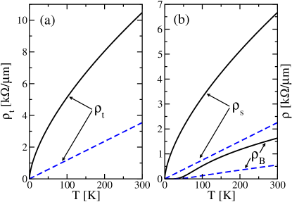
Figure 2: (Color online) (a) Resistivity $\rho_{t}$ of a $(10,10)$ armchair tube caused by coupling to the twiston mode in the noninteracting case ($K_{c+}=1$, blue dashed line) and in the interacting case ($K_{c+}=0.3$, black solid line) with $g_{2}=1.5$ eV. (b) $\rho_{s}$ and $\rho_{B}$ for a $(18,0)$ zigzag tube in the noninteracting case ($K_{c+}=1$, blue dashed line) and in the interacting case ($K_{c+}=0.3$, black solid line) with $g_{2}=1.5$ eV and all other parameters as given in the Appendix B, table 1.

The linear resistivity of the acoustic modes changes into $\rho\sim T^{(1+K_{c+})/2}$ which for $K_{c+}<1$ leads to a negative curvature as a function of temperature. Furthermore, the interactions substantially increase the resistivity by about a factor of $3$ at room temperature in the examples shown in Fig. 2. The contribution of the breathing mode for the zigzag tube is significantly increased by electron-electron interactions as well.

For a comparison with experiment we will concentrate here on the results obtained in Ref. Purewal et al., 2007. In this work single-wall carbon nanotubes with lengths up to $1$ mm were deposited on a Si/SiO₂ substrate and the resistance of a single tube as a function of temperature and length was studied. Except for low temperatures where impurities and possibly localization effects play an important role, the resistance was found to scale linearly with length. We will focus here on device ‘M1’ from Ref. Purewal et al., 2007 which seems to have the cleanest contacts and is metallic down to low temperatures. The resistivity of this device as a function of temperature is shown in Fig. 3 where we have subtracted a small constant contribution due to non-ideal contacts and impurities.

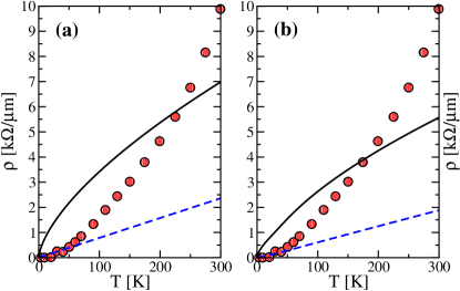
Figure 3: (Color online) Experimental data taken from Ref. Purewal et al., 2007 (dots) compared to theoretical results for (a) a $(15,15)$ armchair and (b) a $(27,0)$ zigzag tube. Results with $g_{2}=1.5$ eV in the non-interacting case $K_{c+}=1$ (blue dashed lines) and in the interacting case with $K_{c+}=0.3$ (black solid lines) are shown.

While scattering at impurities and at the contacts is expected to be relevant and therefore lead to an increasing resistivity for $T\to 0$ at temperatures $T\ll T_{K}$ this temperature regime has not been reached in experiment and taking this contribution as constant seems to be a reasonable approximation. The diameter of the tube in device ‘M1’ has been determined to be $d\approx 2$ nm. The chiral angle, however, is not known. If the tube would be an armchair tube, then this diameter is consistent with a $(15,15)$ tube while a zigzag tube of this diameter would be close to a $(27,0)$ tube. We thus plot in Fig. 3 the theoretical results for both kinds of tubes in comparison to the experimental data.

Including the electron-electron interactions substantially increases the resistivity and leads to a much better overall quantitative agreement with experiment. This is, in particular, true if we assume an armchair tube, Fig. 3(a). Here the deviation between the theoretical curve and the experimental data is never larger than $2-3$ k$\Omega/\mu$m. Treating the electrons as non-interacting, on the other hand, gives a deviation which increases with temperature and is of the order of $7$ k$\Omega/\mu$m at $T=300$ K. Qualitatively however, $\rho(T)\sim T^{(1+K_{c+})/2}$, in the approximation used and with $K_{c+}<1$, gives a concave function while the experimental curve is convex. In the zero temperature limit, the theoretically calculated $\rho(T)$ then has, in particular, infinite slope contrary to what is observed experimentally. Here it is, however, important to note that our approximation, using an infinite wire to calculate $\gamma$, breaks down for $\xi_{e}\gtrsim L$, i.e., $T<T_{c}\approx 30$ K. In the limit $T\to 0$ the properties will be instead dominated by the leads and we have to essentially use the free electron Green’s function in (24) so that the theoretical curve has to smoothly connect to the non-interacting result in this limit.

The relevant microscopic parameters such as the electron-phonon coupling $g_{2}$ or the Luttinger parameter $K_{c+}$ are only approximately known while the chiral angle $\eta$ is even completely undetermined. We can thus try to improve the agreement with experiment by varying these parameters within a reasonable range. The measurements of the tunnel conductanceBockrath et al. (1997); Yao et al. (1999) seem to be convincing evidence that single wall carbon nanotubes are Luttinger liquids with $K_{c+}\approx 0.2-0.4$. In the experiment considered here this nanotube sits on an insulating substrate so there is no reason to expect that $K_{c+}$ is significantly changed by screening effects. For the coupling constant $g_{2}$, on the other hand, estimates obtained from experimental data and theoretical calculations vary between $g_{2}\sim 1-3$ eV.Hertel and Moos (2000); Pietronero et al. (1980); Martino and Egger (2003) Since $g_{2}$ enters quadratically into the resistivity formulas this means that we can vary $\rho(T)$ by almost an order of magnitude. A variation of the chiral angle $\eta$ for a tube with fixed diameter has a substantial effect on the resistivity as well as we have already demonstrated in Fig. 3(a,b). However, as long as we keep $K_{c+}<1$ the temperature dependence will never fully agree with the experimentally observed one.

Finally, we might try to fit the experimental data by assuming that the acoustic modes are quenched and the resistivity is caused purely by a coupling to the breathing mode.

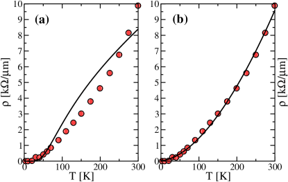
Figure 4: (Color online) Experimental data taken from Ref. Purewal et al., 2007 (dots) compared to: (a) the theoretical results for the breathing mode of a $(27,0)$ zigzag tube assuming $K_{c+}=0.4$, $g_{2}=4.5$ eV, and $\hbar\omega_{B}/k_{B}=250$ K. (b) a fit to a power law yielding $\rho(T)=2770\frac{\text{k}\Omega}{\mu\text{m}}(\pi ak_{B}T/v_{F}\hbar)^{1.73}$.

The result of such a fit is shown in Fig. 4(a) but the electron-phonon coupling $g_{2}=4.5$ eV needed is substantially larger than the largest estimates. This scenario thus seems unrealistic and the fit is not too convincing either. On the other hand, we can obtain an excellent fit of the data over the whole temperature range with a single power law as shown in Fig. 4(b). The exponent obtained in this fit is larger by about $1$ compared to the exponent obtained from the theoretical calculation at $T\gg T_{c}$ for the twiston and stretching contributions. Interestingly, we can obtain such a power law where even the prefactor is of the right magnitude by multiplying our result (IV.1) for the resistivity due to the twiston mode with the characteristic phonon scale, $\rho(T)\to\rho(T)\,k_{B}Ta/(v_{t}\hbar)$. While this could be accidental, the fact that a single power law yields an excellent fit over a wide temperature range and that the damping due to the phononic degrees of the tube gives a resistivity of the right magnitude is a strong indication that this is indeed the dominant mechanism although the theory so far cannot fully explain the temperature scaling. We will speculate about possible modifications of this theory and discuss alternative explanations which can be found in the literature in the conclusions.

V Conclusions

The purpose of this paper has been twofold: On the one hand, we wanted to derive a general formula for the conductance of an interacting quantum wire with good contacts and current relaxing processes in the wire. On the other hand, we wanted to qualitatively understand the temperature and length-dependent scaling of the conductance measured in a recent experimentPurewal et al. (2007) on single wall carbon nanotubes.

Concerning the first part, we have shown that the approach by Maslov and StoneMaslov and Stone (1995) for an interacting ballistic wire contacted to leads can be generalized to an interacting wire with damping. Under the assumptions that a Luttinger liquid description is valid and that the current relaxing processes are predominantly taking part in the bulk of the wire, we were able to give the result for the electronic Green’s function for such a setup in closed form. This allowed us, in particular, to calculate the dc resistance which turned out to consist of two terms. The first is the quantum resistance multiplied by the Luttinger parameter $K_{\ell}$ of the leads. As in the case without damping, there is thus no renormalization if we assume Fermi liquid leads, $K_{\ell}=1$. The second term is proportional to the length of the wire and the damping rate $\gamma$. While this general structure seems obvious, the important point is that $\gamma$, in this approximation, depends only on the Luttinger parameter in the wire $K_{\mathrm{w}}$. We thus have a separation into a constant term, the quantum resistance, which only depends on the properties of the leads, and a term proportional to the length which only depends on the properties of the wire.

As a first application, we have calculated the resistance of an interacting quantum wire which has coexisting ballistic and diffusive channels. Such a coexistence is expected for integrable models where part of the current is protected by a local or quasi-local conservation law.Sirker et al. (2011); Prosen (2011) We find that in such a case the ballistic channel, however small, completely dominates the transport so that the system still shows ideal quantum conductance. However, it is important to mention that two assumptions have been made which cannot be fulfilled in practice: (1) Attaching an integrable wire to contacts will, in general, lead to non-integrable boundary conditions. (2) There will also be relevant backscattering at the contacts which we have neglected. Nevertheless, what this calculation does show is that a quantum wire which has an almost ballistic transport channel can display a conductance which stays close to the ideal quantum conductance over a wide temperature range.

In the second part of the paper we have calculated the resistance of single-wall carbon nanotubes caused by a coupling to the phononic degrees of freedom of the tube. It is well known that there are three modes which have to be taken into account.Suzuura and Ando (2002); Martino and Egger (2003) These are an acoustic twist- and stretching mode as well as an optical breathing mode. Previously, only the contribution of the twiston mode, which is the only one of the three modes active for an armchair tube, had been considered. If one assumes that the electrons are non-interacting then the coupling of the electrons to the twist distortions of the tube leads to a resistivity which increases linearly with temperature.Kane et al. (1998) Interactions, however, are expected to change this temperature dependence.Komnik and Egger (1999) In our paper we have calculated the contribution of all three modes by using a Luttinger liquid theory for the electrons and including the electron-phonon coupling in terms of a self-energy—obtained in second order perturbation theory—for the current-current correlation function. The result depends only on microscopic parameters of the CNT which mostly are relatively well known. A comparison with experiment shows that our results, which do take the electron-electron interactions into account, agree quantitatively better with experiment than the formula for non-interacting electrons. However, qualitatively the observed temperature dependence of the resistivity is different from the calculated one. For temperatures $T$ such that the coherence length $\xi_{e}\ll L$ we find $\rho\sim T^{\alpha}$ with an exponent $\alpha=(1+K_{c+})/2$ determined by the Luttinger parameter of the total charge mode which theoretically and experimentally has been estimated to be around $K_{c+}=0.2-0.4$Egger and Gogolin (1997); Bockrath et al. (1997); Yao et al. (1999) leading to $\alpha=0.6-0.7$. The experimental data, on the other hand, are described extremely well by a power law with exponent $\alpha\approx 1.7$.

Let us discuss possible reasons for these deviations and alternative explanations in the following. First, there is no reason to expect that $K_{c+}$ substantially deviates from the used value. In the experiment the tube is placed on an insulating substrate so that screening should not take place. Interactions with phonons can lead to a renormalization of $K_{c+}$ but are only effective if the Coulomb interaction is already screened.Martino and Egger (2003) A renormalization to values leading to the observed exponent $\alpha\approx 1.7$ is out of the question in any case. Since Luttinger liquid properties have been theoretically predictedEgger and Gogolin (1997) and experimentally observedBockrath et al. (1997); Yao et al. (1999) there seems to be no good reason to doubt the electronic part of our theory. This leaves the phononic part. There is a damping of the phonons due to phonon-phonon interactions which will modify the phonon propagator.De Martino et al. (2009) However, this does not have any effect on our calculations since we are always effectively in a high temperature regime for the acoustic phonons because the sound velocities of the two acoustic modes are much smaller than the Fermi velocity. The phonon modes are therefore always heavily populated and the phonon propagator simply becomes $D(q,\tau)\propto T$ to leading order even if damping is included.

In several papers the possibility of a Peierls distortion of the CNT has been discussed.Sédéki et al. (2000); Mintmire et al. (1992); Figge et al. (2001) If we have a distortion which leads to a finite expectation value of one of the acoustic modes, $\langle\partial_{x}\Phi\rangle\neq 0$ in Eq. (29), then we can easily obtain the temperature dependence of the resistivity in the perturbative regime by scaling arguments. To obtain the self-energy in this case we now have to integrate over time and space and there is a factor of $T$ missing which before came from the phonon propagator. The scaling is therefore given by $\rho\sim T^{(K_{c+}-3)/2}$ in the perturbative regime while $\rho(T)$ will show thermally activated behavior at very low temperatures in the presence of a Peierls distortion. None of this is seen in the experimental data.

If the tube is exactly at half-filling then purely electronic Umklapp scattering is also possible.Balents and Fisher (1997) Note that the same term is called a forward scattering term in Ref. Egger and Gogolin, 1997. The three Umklapp operators in bosonized form are given by $\hat{O}_{U}\sim\cos(4q_{F}x+2\sqrt{\pi}\phi_{c+})\cos(2\sqrt{\pi}\phi_{j\delta})$ with $j\delta\neq c+$. Calculating again the self-energy for such a process in the perturbative regime and using scaling arguments we find that the resistivity due to Umklapp scattering scales as $\rho\sim T^{2K_{c+}-1}$. In particular, the temperature dependence is linear in the non-interacting case, $K_{c+}=1$, as already stated in Ref. Balents and Fisher, 1997. At very low temperatures Umklapp scattering at half-filling will lead to gaps both in the charge and in the spin sector and thus to thermally activated behavior for $\rho(T)$. In a device configuration the filling in the tube is, however, usually tuned away from half-filling so that the Umklapp term oscillates with $4q_{F}$ and can thus be neglected at temperatures $k_{B}T\ll\hbar v_{F}q_{F}$. Even if Umklapp scattering does contribute at higher temperatures its contribution will be smaller by a factor $R_{a}^{-1}$ compared to the electron-phonon contribution so that for the tubes considered here the latter will always be dominant.

There is an alternative explanation for the resistivity of CNTs on surfaces which can be found in the literature.Chandra et al. (2011); Perebeinos et al. (2009) According to these papers the main contribution to the resistivity at room temperature stems from a coupling of the electrons to surface modes of the substrate. The experimental data are explained by combining the resistivity due to the coupling to the acoustic modes of the tube, which dominates at low temperatures, with the resistivity stemming from a coupling to the optical surface modes which yield the main contribution at higher temperatures. In the calculation of both contributions the electrons are treated as non-interacting. This assumption seems questionable. Our calculation shows that once electron-electron interactions are included the interactions with the phonon modes of the tube alone give a resistivity of the right magnitude even at room temperature if standard parameters for the tube are used. If surface modes do indeed give the dominant contribution at room temperature then this would therefore require that the contribution due to the phonon modes of the tube is much smaller than expected. In particular, such a scenario requires $g_{2}\lesssim 0.5$ eV.

While our results provide a much better description of the experimental data than a non-interacting theory, the observed deviations have to remain as an interesting unsolved puzzle. A first step to resolve it would be experiments on free-standing tubes to see if the resistance substantially changes compared to the ones with the tube on a substrate which we considered here.

Appendix A Green’s function for a quantum wire with contacts and damping

To calculate the Green’s function for the action (8) the equation (10) together with the boundary conditions have to be solved. There is a discontinuity in the derivative of $g_{m}$ at $x=x^{\prime}$:

$$\frac{v_{x}}{K_{x}}\partial_{x}g_{m}(x,x^{\prime})|_{x=x^{\prime}-0}^{x=x^{\prime}+0}=1.$$ (41)

For the boundaries at $y=0,L$ we have furthermore

$$\frac{v_{x}}{K_{x}}\partial_{x}g_{m}(x,x^{\prime})|_{x=y-0}^{x=y+0}=0.$$ (42)

where $x\neq x^{\prime}$. $g_{m}(x,x^{\prime})$ itself must be continuous everywhere. We have also fixed $\lim_{x\to\pm\infty}g_{m}(x,x^{\prime})\to 0$. Note that $g_{m}(x,x^{\prime})$ must be symmetric under swapping $x$ and $x^{\prime}$. For $x$ in the three different regions and focusing on $0<x^{\prime}<L$ we make the ansatz

$$g_{m}(x,x^{\prime})=\left\{\begin{array}[]{cc}A\text{e}^{\,\frac{|\omega_{m}|x}{v_{\ell}}}&x<0\\ B\text{e}^{\frac{\omega_{m\gamma}x}{v_{\mathrm{w}}}}+C\text{e}^{-\frac{\omega_{m\gamma}x}{v_{\mathrm{w}}}}&0<x<x^{\prime}\\ D\text{e}^{\frac{\omega_{m\gamma}x}{v_{\mathrm{w}}}}+E\text{e}^{-\frac{\omega_{m\gamma}x}{v_{\mathrm{w}}}}&x^{\prime}<x<L\\ F\text{e}^{-\frac{|\omega_{m}|x}{v_{\ell}}}&x>L\end{array}\right.$$ (47)

where $\omega_{m\gamma}=\sqrt{\omega^{2}_{m}+2\gamma K_{\mathrm{w}}|\omega_{m}|v_{\mathrm{w}}}$ for the damped case and $\omega_{m\gamma}=\sqrt{(1+K_{\mathrm{w}}v_{\mathrm{w}}y^{-1})\omega_{m}^{2}}$ for the the protected current case.

The boundary conditions then lead to the set of equations

$$A = B+C$$ (48a)

$$B-D = e^{-2\frac{x^{\prime}\omega_{m\gamma}}{v_{\mathrm{w}}}}(E-C)$$ (48b)

$$Fe^{-\frac{|\omega_{m}|L}{v_{\ell}}} = De^{\frac{L\omega_{m\gamma}}{v_{\mathrm{w}}}}+Ee^{-\frac{L\omega_{m\gamma}}{v_{\mathrm{w}}}}$$ (48c)

$$B-C = A\frac{K_{\mathrm{w}}}{K_{\ell}}\frac{|\omega_{m}|}{\omega_{m\gamma}}$$ (48d)

$$Fe^{-\frac{|\omega_{m}|L}{v_{\ell}}} = \frac{K_{\ell}}{K_{\mathrm{w}}}\frac{\omega_{m\gamma}}{|\omega_{m}|}\left[Ee^{-\frac{L\omega_{m\gamma}}{v_{\mathrm{w}}}}-De^{\frac{L\omega_{m\gamma}}{v_{\mathrm{w}}}}\right]$$ (48e)

$$B-D = -\frac{K_{\mathrm{w}}e^{-\frac{x^{\prime}\omega_{m\gamma}}{v_{\mathrm{w}}}}}{2\omega_{m\gamma}}$$ (48f)

For convenience we will define

$$\bar{K}_{\omega}=\frac{K_{\ell}\omega_{m\gamma}+K_{\mathrm{w}}|\omega_{m}|}{K_{\ell}\omega_{m\gamma}-K_{\mathrm{w}}|\omega_{m}|}.$$ (49)

This set of equations is readily solved and one finds

$$B = \frac{K_{\mathrm{w}}\bar{K}_{\omega}}{2\omega_{m\gamma}}\frac{e^{\frac{x^{\prime}\omega_{m\gamma}}{v_{\mathrm{w}}}}+e^{\frac{(2L-x^{\prime})\omega_{m\gamma}}{v_{\mathrm{w}}}}\bar{K}_{\omega}}{1-e^{\frac{2L\omega_{m\gamma}}{v_{\mathrm{w}}}}\bar{K}_{\omega}^{2}}$$ (50a)

$$C = \frac{K_{\mathrm{w}}}{2\omega_{m\gamma}}\frac{e^{\frac{x^{\prime}\omega_{m\gamma}}{v_{\mathrm{w}}}}+e^{\frac{(2L-x^{\prime})\omega_{m\gamma}}{v_{\mathrm{w}}}}\bar{K}_{\omega}}{1-e^{\frac{2L\omega_{m\gamma}}{v_{\mathrm{w}}}}\bar{K}_{\omega}^{2}}$$ (50b)

$$D = \frac{K_{\mathrm{w}}}{2\omega_{m\gamma}}\frac{e^{-\frac{x^{\prime}\omega_{m\gamma}}{v_{\mathrm{w}}}}+e^{\frac{x^{\prime}\omega_{m\gamma}}{v_{\mathrm{w}}}}\bar{K}_{\omega}}{1-e^{\frac{2L\omega_{m\gamma}}{v_{\mathrm{w}}}}\bar{K}_{\omega}^{2}}$$ (50c)

$$E = \frac{K_{\mathrm{w}}\bar{K}_{\omega}}{2\omega_{m\gamma}}\frac{e^{-\frac{x^{\prime}\omega_{m\gamma}}{v_{\mathrm{w}}}}+e^{\frac{x^{\prime}\omega_{m\gamma}}{v_{\mathrm{w}}}}\bar{K}_{\omega}}{e^{-\frac{2L\omega_{m\gamma}}{v_{\mathrm{w}}}}-\bar{K}_{\omega}^{2}}.$$ (50d)

This completes the determination of the parameters in (47) which is thus the full bosonic Green’s function for a quantum wire with contacts and damping in the bulk.

Analytic continuation gives us $\omega_{m}\to-i\omega+\delta$, and defining $\omega_{\gamma}=i\omega_{m\gamma}|_{\omega_{m}=-i\omega}$ and $\bar{K}_{\omega}=\bar{K}_{\omega_{m}=-i\omega}$ we have

$$\omega_{\gamma} = \left\{\begin{array}[]{cc}\sqrt{\omega^{2}+2i\gamma K_{\mathrm{w}}\omega v_{\mathrm{w}}}&\textrm{ or}\\[2.84544pt] \sqrt{(1+K_{\mathrm{w}}v_{\mathrm{w}}y^{-1})\omega^{2}}&\end{array}\right.$$ (53)

where the first line applies to the damped case with self energy $\Sigma\approx-2\text{i}\gamma\omega$ and the second line to the case where part of the current is conserved with a self energy $\Sigma\approx-y^{-1}\omega^{2}$. In addition, we now have

$$\bar{K}_{\omega} = \frac{K_{\ell}\omega_{\gamma}+K_{\mathrm{w}}\omega}{K_{\ell}\omega_{\gamma}-K_{\mathrm{w}}\omega}.$$ (54)

In the low-frequency limit we note that the Green’s function becomes position independent:

$$g(x,x^{\prime};\omega)\approx\frac{iK_{\mathrm{w}}\left(1+\bar{K}_{\omega}\right)}{2\omega_{\gamma}}\frac{1+e^{-\text{i}\frac{2L\omega_{\gamma}}{v_{\mathrm{w}}}}\bar{K}_{\omega}}{1-e^{-\text{i}\frac{2L\omega_{\gamma}}{v_{\mathrm{w}}}}\bar{K}_{\omega}^{2}}.$$ (55)

Now, for the damped case as $\omega\ll\gamma K_{\mathrm{w}}v_{\mathrm{w}}$ we have $\omega_{\gamma}\sim e^{-i\pi/4}\sqrt{2\gamma K_{\mathrm{w}}\omega v_{\mathrm{w}}}$. In the protected current scenario we find in the low-frequency limit

$$g(x,x^{\prime};\omega)\approx\frac{iK_{\mathrm{w}}}{2\omega\sqrt{(1+K_{\mathrm{w}}v_{\mathrm{w}}y^{-1})}}\frac{1+\bar{K}_{\omega}}{1-\bar{K}_{\omega}}\,.$$ (56)

Appendix B Parameters for carbon nanotubes

In Table 1, we list all the relevant microscopic parameters to obtain the resistance of single-wall carbon nanotubes caused by electron-phonon coupling. For some parameters significantly varying estimates have been given in the literature in which cases we give the range of these estimates.

Table 1: Relevant parameters for the resistance of carbon nanotubes

Quantity	Symbol	Value
Lattice constant	$a$	$2.46\cdot 10^{-10}$ m
Carbon mass per unit area	$M$	$3.8\cdot 10^{-7}$ kg/$\text{m}^{2}$
Fermi velocity	$v_{F}$	$8\cdot 10^{5}$ m/s
Radius of a $(n,m)$ tube	$R_{a}$	$\frac{a}{2\pi}\sqrt{n^{2}+nm+m^{2}}$
Bulk modulusDolling and Brockhouse (1962)	$B$	$110.2$ kg/$\text{s}^{2}$
Shear modulusDolling and Brockhouse (1962)	$\mu$	$57.38$ kg/$\text{s}^{2}$
Twiston velocitySuzuura and Ando (2002)	$v_{t}$	$1.23\cdot 10^{4}$ m/s
Twist modulus for $(n,n)$ tubeKane et al. (1998)	$C_{t}$	$n^{3}18\cdot 10^{-10}$ eV m
Twist moment of inertia per unit length	$M_{t}$	$C_{t}/v_{t}^{2}$ [kg m]
Stretching mode velocitySuzuura and Ando (2002)	$v_{s}$	$1.99\cdot 10^{4}$ m/s
Breathing mode frequencySuzuura and Ando (2002)	$w_{B}$	$\sqrt{\frac{B+\mu}{M}}\frac{1}{R_{a}}$ 1/s
Factor between twiston and stretching propagator	$\mathcal{A}$	$\frac{4B-Mv_{s}^{2}}{B+\mu}\left(\frac{v_{t}}{v_{s}}\right)^{2}\approx 0.66$
Quantum resistance	$R_{Q}=\frac{h}{4e^{2}}$	$6.45$ k$\Omega$
Transfer integralSuzuura and Ando (2002)	$\gamma_{0}$	$3.0$ eV
Transfer integral	$\beta$	$1.1$ eVHertel and Moos (2000), $3.6$ eVPietronero et al. (1980)
Electron-phonon coupling constantSuzuura and Ando (2002)	$g_{2}=\frac{3\mu\beta\gamma_{0}}{4\sqrt{2}B}$	$0.91-2.98$ eV; $1.5$ eVMartino and Egger (2003)

References

- Landauer (1957) R. Landauer, IBM J. Res. Div. 1, 223 (1957).
- Kane and Fisher (1992) C. L. Kane and M. P. A. Fisher, Phys. Rev. B 46, 15233 (1992).
- Ogata and Fukuyama (1994) M. Ogata and H. Fukuyama, Phys. Rev. Lett. 73, 468 (1994).
- Tarucha et al. (1995) S. Tarucha, T. Honda, and T. Saku, Solid State Commun. 94, 413 (1995).
- Maslov and Stone (1995) D. L. Maslov and M. Stone, Phys. Rev. B 52, R5539 (1995).
- Safi and Schulz (1995) I. Safi and H. J. Schulz, Phys. Rev. B 52, R17040 (1995).
- Kane et al. (1998) C. L. Kane, E. J. Mele, R. S. Lee, J. E. Fischer, P. Petit, H. Dai, A. Thess, R. E. Smalley, A. R. M. Verschueren, S. J. Tans, et al., EPL 41, 683 (1998).
- Ristivojevic and Nattermann (2008) Z. Ristivojevic and T. Nattermann, Phys. Rev. Lett. 101, 016405 (2008).
- Furusaki and Nagaosa (1996) A. Furusaki and N. Nagaosa, Phys. Rev. B 54, R5239 (1996).
- Sedlmayr et al. (2012) N. Sedlmayr, J. Ohst, I. Affleck, J. Sirker, and S. Eggert, Phys. Rev. B 86, 121302(R) (2012).
- Charlier et al. (2007) J.-C. Charlier, X. Blase, and S. Roche, Rev. Mod. Phys. 79, 677 (2007).
- Kane et al. (1997) C. Kane, L. Balents, and M. P. A. Fisher, Phys. Rev. Lett. 79, 5086 (1997).
- Egger and Gogolin (1997) R. Egger and A. O. Gogolin, Phys. Rev. Lett. 79, 5082 (1997).
- Bockrath et al. (1997) M. Bockrath, D. H. Cobden, P. L. McEuen, N. G. Chopra, A. Zettl, A. Thess, and R. E. Smalley, Science 275, 1922 (1997).
- Bockrath et al. (1999) M. Bockrath, D. H. Cobden, J. Lu, A. G. Rinzler, R. E. Smalley, L. Balents, and P. L. McEuen, Nature 397, 598 (1999).
- Yao et al. (1999) Z. Yao, H. W. C. Postma, L. Balents, and C. Dekker, Nature 402, 273 (1999).
- Yoshioka and Odintsov (1999) H. Yoshioka and A. A. Odintsov, Phys. Rev. Lett. 82, 374 (1999).
- Dóra et al. (2007) B. Dóra, M. Gulácsi, F. Simon, and H. Kuzmany, Phys. Rev. Lett. 99, 166402 (2007).
- Singer et al. (2005) P. M. Singer, P. Wzietek, H. Alloul, F. Simon, and H. Kuzmany, Phys. Rev. Lett. 95, 236403 (2005).
- Purewal et al. (2007) M. S. Purewal, B. H. Hong, A. Ravi, B. Chandra, J. Hone, and P. Kim, Phys. Rev. Lett. 98, 186808 (2007).
- Park et al. (2004) J.-Y. Park, S. Rosenblatt, Y. Yaish, V. Sazonova, H. Üstunel, S. Braig, T. A. Arias, P. W. Brouwer, and P. L. McEuen, Nano Lett. 4, 517 (2004).
- Ilani and McEuen (2010) S. Ilani and P. L. McEuen, Ann. Rev. Cond. Mat. Phys. 1, 1 (2010).
- Balents and Fisher (1997) L. Balents and M. P. A. Fisher, Phys. Rev. B 55, R11973 (1997).
- Giamarchi (2004) T. Giamarchi, Quantum physics in One Dimension (Clarendon Press, Oxford, 2004).
- Sirker et al. (2009) J. Sirker, R. G. Pereira, and I. Affleck, Phys. Rev. Lett. 103, 216602 (2009).
- Sirker et al. (2011) J. Sirker, R. G. Pereira, and I. Affleck, Phys. Rev. B 83, 035115 (2011).
- Soori and Sen (2011a) A. Soori and D. Sen, EPL 93, 57007 (2011a).
- Soori and Sen (2011b) A. Soori and D. Sen, Phys. Rev. B 84, 035422 (2011b).
- Prosen (2011) T. Prosen, Phys. Rev. Lett. 106, 217206 (2011).
- Rosch and Andrei (2000) A. Rosch and N. Andrei, Phys. Rev. Lett. 85, 1092 (2000).
- Sundqvist et al. (2008) P. A. Sundqvist, F. J. Garcia-Vidal, and F. Flores, Phys. Rev. B 78, 205427 (2008).
- Egger et al. (2001) R. Egger, A. Bachthold, M. Fuhrer, M. Bockrath, D. Cobden, and P. McEuen, Lecture Notes in Physics (Springer, 2001), vol. 579, p. 125.
- Dresselhaus and Eklund (2000) M. S. Dresselhaus and P. C. Eklund, Adv. Phys. 49, 705 (2000).
- Suzuura and Ando (2002) H. Suzuura and T. Ando, Phys. Rev. B 65, 235412 (2002).
- Martino and Egger (2003) A. D. Martino and R. Egger, Phys. Rev. B 67, 235418 (2003).
- Chen et al. (2010) W. Chen, A. V. Andreev, E. G. Mishchenko, and L. I. Glazman, Phys. Rev. B 82, 115444 (2010).
- Schulz (1986) H. J. Schulz, Phys. Rev. B 34, 6372 (1986).
- Hertel and Moos (2000) T. Hertel and G. Moos, Phys. Rev. Lett. 84, 5002 (2000).
- Pietronero et al. (1980) L. Pietronero, S. Strässler, H. R. Zeller, and M. J. Rice, Phys. Rev. B 22, 904 (1980).
- Komnik and Egger (1999) A. Komnik and R. Egger, arXiv:cond-mat/9906150 (1999).
- De Martino et al. (2009) A. De Martino, R. Egger, and A. O. Gogolin, Phys. Rev. B 79, 205408 (2009).
- Sédéki et al. (2000) A. Sédéki, L. G. Caron, and C. Bourbonnais, Phys. Rev. B 62, 6975 (2000).
- Mintmire et al. (1992) J. W. Mintmire, B. I. Dunlap, and C. T. White, Phys. Rev. Lett. 68, 631 (1992).
- Figge et al. (2001) M. T. Figge, M. Mostovoy, and J. Knoester, Phys. Rev. Lett. 86, 4572 (2001).
- Chandra et al. (2011) B. Chandra, V. Perebeinos, S. Berciaud, J. Katoch, M. Ishigami, P. Kim, T. F. Heinz, and J. Hone, Phys. Rev. Lett. 107, 146601 (2011).
- Perebeinos et al. (2009) V. Perebeinos, S. V. Rotkin, A. G. Petrov, and P. Avouris, Nano Lett. 9, 312 (2009).
- Dolling and Brockhouse (1962) G. Dolling and B. N. Brockhouse, Phys. Rev. 128, 1120 (1962).