The Discovery of HD 37605$c$ and a Dispositive Null Detection of Transits of HD 37605$b$

Abstract

We report the radial-velocity discovery of a second planetary mass companion to the K0 V star HD 37605, which was already known to host an eccentric, $P\sim 55$ days Jovian planet, HD 37605$b$. This second planet, HD 37605$c$, has a period of $\sim 7.5$ years with a low eccentricity and an $M\sin{i}$ of $\sim 3.4\ M_{\rm Jup}$. Our discovery was made with the nearly 8 years of radial velocity follow-up at the Hobby-Eberly Telescope and Keck Observatory, including observations made as part of the Transit Ephemeris Refinement and Monitoring Survey (TERMS) effort to provide precise ephemerides to long-period planets for transit follow-up. With a total of 137 radial velocity observations covering almost eight years, we provide a good orbital solution of the HD 37605 system, and a precise transit ephemeris for HD 37605$b$. Our dynamic analysis reveals very minimal planet-planet interaction and an insignificant transit time variation. Using the predicted ephemeris, we performed a transit search for HD 37605$b$ with the photometric data taken by the T12 0.8-m Automatic Photoelectric Telescope (APT) and the Microvariability and Oscillations of Stars (MOST) satellite. Though the APT photometry did not capture the transit window, it characterized the stellar activity of HD 37605, which is consistent of it being an old, inactive star, with a tentative rotation period of $57.67$ days. The MOST photometry enabled us to report a dispositive null detection of a non-grazing transit for this planet. Within the predicted transit window, we exclude an edge-on predicted depth of 1.9% at the $\gg 10\sigma$ level, and exclude any transit with an impact parameter $b>0.951$ at greater than $5\sigma$. We present the BOOTTRAN package for calculating Keplerian orbital parameter uncertainties via bootstrapping. We made a comparison and found consistency between our orbital fit parameters calculated by the RVLIN package and error bars by BOOTTRAN with those produced by a Bayesian analysis using MCMC.

1. Introduction

1.1. Context

Jupiter analogs orbiting other stars represent the first signposts of true Solar System analogs, and the eccentricity distribution of these planets with $a>3$ AU will reveal how rare or frequent true Jupiter analogs are. To date, only 9 “Jupiter analogs” have been well-characterized in the peer reviewed literature (defined here as $P>8$ years, $4>M\sin{i}>0.5\ M_{\rm Jup}$, and $e<0.3$; Wright et al., 2011, exoplanets.org). As the duration of existing planet searches approach 10–20 years, more and more Jupiter analogs will emerge from their longest-observed targets (Wittenmyer et al., 2012; Boisse et al., 2012).

Of the over 700 exoplanets discovered to date, nearly 200 are known to transit their host star (Wright et al. 2011, exoplanets.org; Schneider et al. 2011, exoplanet.eu), and many thousands more candidates have been discovered by the Kepler telescope. Of all of these planets, only three orbit stars with $V<8$ and all have $P<4$ days. Long period planets are less likely than close-in planets to transit unless their orbits are highly eccentric and favorably oriented, and indeed only 2 transiting planets with $P>20$ days have been discovered around stars with $V<10$, and both have $e>0.65$ (HD 80606, Laughlin et al. 2009, Fossey et al. 2009; HD 17156, Fischer et al. 2007, Barbieri et al. 2007; both highly eccentric systems were discovered first with radial velocities).

Long period planets not known to transit can have long transit windows due to both the large duration of any edge-on transit and higher phase uncertainties (since such uncertainties scale with the period of the orbit). Long term radial velocity monitoring of stars, for instance for the discovery of low amplitude signals, can produce collateral benefits in the form of orbit refinement for a transit search and the identification of Jupiter analogs (e.g., Wright et al., 2009). Herein, we describe an example of both.

1.2. Initial Discovery and Followup

The inner planet in the system, HD 37605$b$, was the first planet discovered with the Hobby-Eberly Telescope (HET) at McDonald Observatory (Cochran et al., 2004). It is a super Jupiter ($M\sin{i}=2.41\ M_{\rm Jup}$) on an eccentric orbit $e=0.67$ with an orbital period in the “period valley” ($P=55$ days; Wright et al., 2009).

W.C., M.E., and P.J.M.  of the University of Texas at Austin, continued observations in order to get a much better orbit determination and to begin searching for transits. With the first new data in the fall of 2004, it became obvious that another perturber was present in the system, first from a trend in the radial velocity (RV) residuals (i.e., a none-zero $\mbox{d}v/\mbox{d}t$; Wittenmyer et al., 2007), and later from curvature in the residuals. By 2009, the residuals to a one-planet fit were giving reasonable constraints on the orbit of a second planet, HD 37605$c$, and by early 2011 the orbital parameters of the $c$ component were clear, and the Texas team was preparing the system for publication.

1.3. TERMS Data

The Transit Ephemeris Refinement and Monitoring Survey (TERMS; Kane et al., 2009) seeks to refine the ephemerides of the known exoplanets orbiting bright, nearby stars with sufficient precision to efficiently search for the planetary transits of planets with periastron distances greater than a few hundredths of an AU (Kane et al., 2011b; Pilyavsky et al., 2011a; Dragomir et al., 2011). This will provide the radii of planets not experiencing continuous high levels of insolation around nearby, easily studied stars.

In 2010, S.M. and J.T.W. began radial velocity observations of HD 37605$b$ at HET from Penn State University for TERMS, to refine the orbit of that planet for a future transit search. These observations, combined with Keck radial velocities from the California Planet Survey (CPS) consortium from 2006 onward, revealed that there was substantial curvature to the radial velocity residuals to the original Cochran et al. (2004) solution. In October 2010 monitoring was intensified at HET and at Keck Observatory by A.W.H., G.W.M., J.T.W., and H.I., and with these new RV data and the previously published measurements from Wittenmyer et al. (2007) they obtained a preliminary solution for the outer planet. The discrepancy between the original orbital fit and the new fit (assuming one planet) was presented at the January 2011 meeting of the American Astronomical Society (Kane et al., 2011c).

1.4. Synthesis and Outline

In early 2011, the Texas and TERMS teams combined efforts and began joint radial velocity analysis, dynamical modeling, spectroscopic analysis, and photometric observations (Kane et al., 2012). The resulting complete two-planet orbital solution allows for a sufficiently precise transit ephemeris for the $b$ component to be calculated for a thorough transit search. We herein report the transit exclusion of HD 37605$b$ and a stable dynamical solution to the system.

In § 2, we describe our spectroscopic observations and analysis, which provided the radial velocities and the stellar properties of HD 37605. § 3 details the orbital solution for the HD 37605 system, including a comparison with MCMC Keplerian fits, and our dynamical analysis. We report our photometric observations on HD 37605 and the dispositive null detection of non-grazing transits of HD 37605$b$ in § 4. After § 5, Summary and Conclusion, we present updates on $M\sin{i}$ of two previously published systems (HD 114762 and HD 168443) in § 6. In the Appendix we describe the algorithm used in the package BOOTTRAN (for calculating orbital parameter error bars; see § 3.2).

2. Spectroscopic Observations and Analysis

2.1. HET and Keck Observations

Observations on HD 37605 at HET started December of 2003. In total, 101 RV observations took place over the course of almost eight years, taking advantage of the queue scheduling capabilities of HET. The queue scheduling of HET allows for small amounts of telescope time to be optimally used throughout the year, and for new observing priorities to be implemented immediately, rather than on next allocated night or after TAC and scheduling process (Shetrone et al., 2007). The observations were taken through the High Resolution Spectrograph (HRS; Tull, 1998) situated at the basement of the HET building. This fiber-fed spectrograph has a typical long-term Doppler error of 3 – 5 m s^-1 (Baluev, 2009). The observations were taken with the spectrograph configured at a resolving power of $R=$60,000. For more details, see Cochran et al. (2004).

Observations at Keck were taken starting August 2006. A set of 33 observations spanning over five years were made through the HIRES spectrometer (Vogt et al., 1994) on the Keck I telescope, which has a long-term Doppler error of 0.9 – 1.5 m s^-1 (e.g. Howard et al., 2009). The observations were taken at a resolving power of $R=$55,000. For more details, see Howard et al. (2009) and Valenti et al. (2009).

Both our HET and Keck spectroscopic observations were taken with an iodine cell placed in the light path to provide wavelength standard and information on the instrument response function (IRF) for radial velocity extraction (Marcy & Butler, 1992; Butler et al., 1996). In addition, we also have observations taken without iodine cell to produce stellar spectrum templates – on HET and Keck, respectively. The stellar spectrum templates, after being deconvolved with the IRF, are necessary for both radial velocity extraction and stellar property analysis. The typical working wavelength range for this technique is roughly 5000 Å– 6000 Å.

2.2. Data Reduction and Doppler Analysis

In this section, we describe our data reduction and Doppler analysis of the HET observations. We reduced the Keck data with the standard CPS pipeline, as described in, for example, Howard et al. (2011) and Johnson et al. (2011b).

We have constructed a complete pipeline for analyzing HET data – from raw data reduction to radial velocity extraction. The raw reduction is done using the REDUCE package by Piskunov & Valenti (2002). This package is designed to optimally extract echelle spectra from 2-D images (Horne, 1986). Our pipeline corrects for cosmic rays and scattered light. In order to make the data reduction process completely automatic, we have developed our own algorithm for tracing the echelle orders of HRS and replaced the original semi-automatic algorithm from the REDUCE package.

After the raw data reduction, the stellar spectrum template is deconvolved using IRF derived from an iodine flat on the night of observation. There were two deconvolved stellar spectrum templates (DSST) derived from HET/HRS observations and one from Keck/HIRES. Throughout this work, we use the Keck DSST, which is of better quality thanks to a better known IRF of HIRES and a superior deconvolution algorithm in the CPS pipeline (Howard et al., 2009, 2011).

Then the pipeline proceeds with barycentric correction and radial velocity extraction for each observation. We have adopted the Doppler code from CPS (e.g. Howard et al., 2009, 2011; Johnson et al., 2011b). The code is tailored to be fully functional with HET/HRS-formatted spectra, and it is capable of working with either an HET DSST or a Keck one.

The 101 HET RV observations include 44 observations which produced the published velocities in Cochran et al. (2004) and Wittenmyer et al. (2007), 34 observations also done by the Texas team in follow-up work after 2007, and 23 observations taken as part of TERMS program. We have performed re-reduction on these 44 observations together with all the rest 57 HET observations through our pipeline. This has the advantage of eliminating one free parameter in the Keplerian fit – the offset between two Doppler pipelines.

Two out of the 101 HET observations were excluded due to very low average signal-to-noise ratio per pixel ($<20$), and one observation taken at twilight was also rejected as such observation normally results in low accuracy due to the significant contamination by the residual solar spectrum (indeed this velocity has a residual of over $100$ m s^-1 against best Keplerian fit, much larger than the $\sim 8$ m s^-1 RV error).

All the HET and Keck radial velocities used in this work (98 from HET and 33 from Keck) are listed in Table 7.

2.3. Stellar Analysis

Table 1STELLAR PARAMETERS

Parameter	Value
Spectral type	K0 V
Distance (pc)	44.0 $\pm$ 2.1
$V$	8.661 $\pm$ 0.013
$T_{\mbox{eff}}$ (K)	5448 $\pm$44
$\log{g}$	4.511 $\pm$ 0.024
$[$Fe/H$]$	0.336 $\pm$ 0.030
BC	-0.144
$M_{\mbox{bol}}$	5.301
$L_{\star}$ ($L_{\odot}$)	0.590 $\pm$ 0.058
$R_{\star}$ ($R_{\odot}$)	0.901 $\pm$ 0.045
$M_{\star}$ ($M_{\odot}$)	1.000 $\pm$ 0.050
$v\sin{i}$	$<1$ km s-1
Age	$\sim 7$ Gyr

HD 37605 is a K0 V star (V $\sim$ 8.7) with high proper motion at a distance of 44.0 $\pm$ 2.1 pc (ESA, 1997; van Leeuwen, 2008). We derived its stellar properties based on analysis on a high-resolution spectrum taken with Keck HIRES (without iodine cell in the light path). Table 1 lists the results of our analysis, including the effective temperature $T_{\rm eff}$, surface gravity $\log{g}$, iron abundance $[{\rm Fe/H}]$, projected rotational velocity $v\sin{i}$, bolometric correction BC, bolometric magnitude $M_{\rm bol}$, stellar luminosity $L_{\star}$, stellar radius $R_{\star}$, stellar mass $M_{\star}$ and age. HD 37605 is found to be a metal rich star ($[{\rm Fe/H}]\sim 0.34$) with $M_{\star}\sim 1.0\ M_{\odot}$ and $R_{\star}\sim 0.9R_{\odot}$.

We followed the procedure described in Valenti & Fischer (2005) and also in Valenti et al. (2009) with improvements. Briefly, the observed spectrum is fitted with a synthetic spectrum using Spectroscopy Made Easy (SME; Valenti & Piskunov, 1996) to derive $T_{\rm eff}$, $\log{g}$, $[{\rm Fe/H}]$, $v\sin{i}$, and so on, which are used to derive the bolometric correction BC and $L_{\star}$ consequently. Then an isochrone fit by interpolating tabulated Yonsei-Yale isochrones (Demarque et al., 2004) using derived stellar parameters from SME is performed to calculate $M_{\star}$ and $\log{g_{\rm iso}}$ values (along with age and stellar radius). Next, Valenti et al. (2009) introduced an outside loop which re-runs SME with $\log{g}$ fixed at $\log{g_{\rm iso}}$, followed by another isochrone fit deriving a new log $\log{g_{\rm iso}}$ using the updated SME results. The loop continues until $\log{g}$ values converge. This additional iterative procedure to enforce self-consistency on log $g$ is shown to improve the accuracy of other derived stellar parameters (Valenti et al., 2009). The stellar radius and $\log{g}$ reported here in Table 1 are derived from the final isochrone fit, which are consistent with the purely spectroscopic results. The gravity ($\log{g}=4.51$) is also consistent with the purely spectroscopic gravity ($4.44$) based on strong Mg b damping wings, so for HD 37605 the iteration process is optional.

Cochran et al. (2004) reported the values of $T_{\rm eff}$, $\log{g}$, and $[$Fe/H$]$ for HD 37605, and their estimates agree with ours within 1$\sigma$ uncertainty. Santos et al. (2005) also estimated $T_{\rm eff}$, $\log{g}$, $[$Fe/H$]$, and $M_{\star}$, all of which agree with our values within 1$\sigma$. Our stellar mass and radius estimates are also consistent with the ones derived from the empirical method by Torres et al. (2010).

Our SME analysis indicates that the rotation of the star ($v\sin{i}$) is likely $<1$ km s^-1 (corresponding to rotation period $\gtrsim 46$ days). We have used various methods to estimate stellar parameters from the spectrum, including the incorporation of color and absolute magnitude information and the Mg b triplet to constrain $\log{g}$, and various macroturbulent velocity prescriptions. All of these approaches yield results consistent with an undetectable level of rotational broadening, with an upper limit of 1-2 km s^-1, consistent with the tentative photometric period 57.67 days derived from the APT data (See §4.1).

3. Orbital Solution

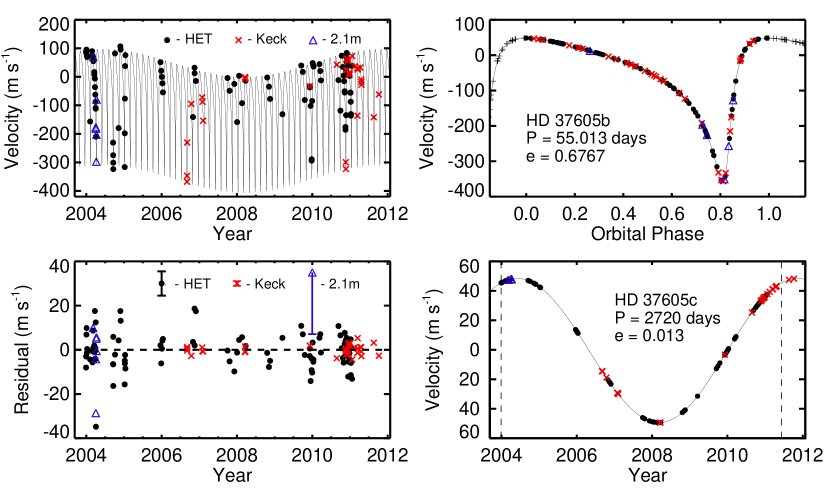
Figure 1.— Radial velocity and Keplerian model plots for the HD 37605 system. In all panels, HET observations are labeled with black filled circles, Keck observations are labeled with red crosses, and the velocities from the 2.1 m telescope (Cochran et al., 2004) are labeled with blue triangles. Best Keplerian fits are plotted in black solid lines. Top left: The best-fit 2-planet Keplerian model (solid line) and the observed radial velocities from 3 telescopes. The HET and Keck velocities have been adjusted to take into account the velocity offsets (i.e., subtracting $\Delta_{\rm HET}$ and $\Delta_{\rm Keck}$ from the velocities, respectively; see Table 2 and § 3.2). Bottom left: Residual velocities after subtracting the best-fit 2-planet Keplerian model. The lengend gives the typical size of the error bars using the $\pm$ median RV error for each telescope (for 2.1 m telescope only the lower half is shown). Top right: RV signal induced by HD 37605$b$ alone, phased up to demonstrate our coverage. Bottom right: RV signal induced by HD 37605$c$ alone. The two vertical dashed lines denote the date of our first observation, and the date when HD 37605$c$ closes one orbit, respectively. (A color version of this figure is available in the online journal.)

3.1. Transit Ephemeris

The traditional parameters for reporting the ephemerides of spectroscopic binaries are $P,K,e,\omega$, and $T_{p}$, the last being the time of periastron passage (Wright & Howard, 2009). This information is sufficient to predict the phase of a planet at any point in the future in principle, but the uncertainties in those parameters alone are insufficient to compute the uncertainty in orbital phase without detailed knowledge of the covariances among the parameters.

This problem is particularly acute when determining transit or secondary eclipse times for planets with near circular orbits, where $\sigma_{T_{p}}$ and $\sigma_{\omega}$ can be highly covariant. In such cases the circular case is often not excluded by the data, and so the estimation of $e$ includes the case $e=0$, where $\omega$ is undefined. If the best or most likely value of $e$ in this case is small but not zero, then it is associated with some nominal value of $\omega$, but $\sigma_{\omega}$ will be very large (approaching $\pi$). Since $T_{p}$ represents the epoch at which the true anomaly equals $0$, $T_{p}$ will have a similarly large uncertainty (approaching $P$), despite the fact that the phase of the system may actually be quite precisely known!

In practice even the ephemerides of planets with well measured eccentricities suffer from lack of knowledge of the covariance in parameters, in particular $T_{p}$ and $P$ (whose covariance is sensitive to the approximate epoch chosen for $T_{p}$). To make matters worse, the nature of “1$\sigma$” uncertainties in the literature is inconsistent. Some authors may report uncertainties generated while holding all or some other parameters constant (for instance, by seeing at what excursion from the nominal value $\chi^{2}$ is reduced by 1), while others using bootstrapping or MCMC techniques may report the variance in a parameter over the full distribution of trials. In any case, covariances are rarely reported, and in some cases authors even report the most likely values on a parameter-by-parameter basis rather than a representative “best fit”, resulting in a set of parameters that is not self-consistent.

The TERMS strategy for refining ephemerides therefore begins with the recalculation of transit time uncertainties directly from the archival radial velocity data. We used bootstrapping (see Appendix) with the time of conjunction, $T_{c}$ (equivalent to transit center, in the case of transiting planets) computed independently for each trial. For systems whose transit time uncertainty makes definitive observations implausible or impossible due to the accumulation of errors in phase with time, we sought additional RV measurements to “lock down” the phase of the planet.

3.2. The 37605 System

There are in total 137 radial velocities used in the Keplerian fit for the HD 37605 system. In addition to the 98 HET velocities and 33 Keck ones (see §2.2), we also included six velocities from Cochran et al. (2004) which were derived from observations taken with the McDonald Observatory 2.1 m Telescope (hereafter the 2.1 m telescope).

We used the RVLIN package by Wright & Howard (2009) to perform the Keplerian fit. This package is based on the Levenberg–Marquardt algorithm and is made efficient in searching parameter space by exploiting the linear parameters. The uncertainties of the parameters are calculated through bootstrapping (with $1,000$ bootstrap replicates) using the BOOTTRAN package, which is described in detail in the Appendix.

The best-fit Keplerian parameters are listed in Table 2. The joint Keplerian fit for HD 37605$b$ and HD 37605$c$ has 13 free parameters: the orbital period $P$, time of periastron passage $T_{p}$, velocity semi-amplitude $K$, eccentricity $e$, and the argument of periastron referenced to the line of nodes $\omega$ for each planet; and for the system, the velocity offset between the center of the mass and barycenter of solar system $\gamma$ and two velocity offsets between the three telescopes ($\Delta_{\rm Keck}$ and $\Delta_{\rm HET}$, with respect to the velocities from the 2.1 m telescope as published in Cochran et al. 2004). We did not include any stellar jitter or radial velocity trend in the fit (i.e., fixed to zero). The radial velocity signals and the best Keplerian fits for the system, HD 37605$b$ only, and HD 37605$c$ only are plotted in the three panels of Fig. 1, respectively.

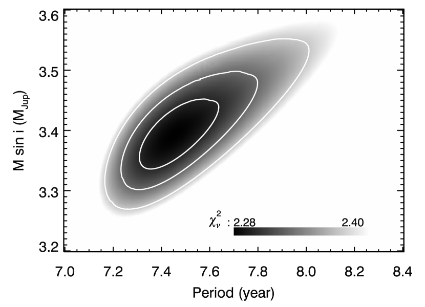
Figure 2.— $\chi^{2}_{\nu}$ map for the best Keplerian fits with fixed values of period $P$ and minimum planet mass $M\sin{i}$ for HD 37605$c$. This is showing that both $P$ and $M\sin{i}$ are well-constrained for this planet. The levels of the contours mark the 1$\sigma$ (68.27%), 2$\sigma$ (95.45%) and 3$\sigma$ (99.73%) confidence intervals for the 2-D $\chi^{2}$ distribution.

Adopting a stellar mass of $M_{\star}=1.000\pm 0.017\ M_{\odot}$ (as in Table 1), we estimated the minimum mass ($M\sin{i}$) for HD 37605$b$ to be $2.802\pm 0.011\ M_{\rm Jup}$ and $3.366\pm 0.072\ M_{\rm Jup}$ for HD 37605$c$. While HD 37605$b$ is on a close-in orbit at $a=0.2831\pm 0.0016$ AU that is highly eccentric ($e=0.6767\pm 0.0019$), HD 37605$c$ is found to be on a nearly circular orbit ($e=0.013\pm 0.015$) out at $a=3.814\pm 0.058$ AU, which qualifies it as one of the “Jupiter analogs”.

In order to see whether the period and mass of the outer planet, HD 37605$c$, are well constrained, we mapped out the $\chi_{\nu}^{2}$ values for the best Keplerian fit in the $P_{c}$-$M_{c}\sin{i}$ space (subscript ‘$c$’ denoting parameters for the outer planet, HD 37605$c$). Each $\chi_{\nu}^{2}$ value on the $P_{c}$-$M_{c}\sin{i}$ grid was obtained by searching for the best-fit model while fixing the period $P_{c}$ for the outer planet and requiring constraints on $K_{c}$ and $e_{c}$ to maintain $M\sin{i}$ fixed. As shown in Fig. 2, our data are sufficient to have both $P_{c}$ and $M_{c}\sin{i}$ well-constrained. This is also consistent with the tight sampling distributions for $P_{c}$ and $M_{c}\sin{i}$ found in our bootstrapping results.

The rms values against the best Keplerian fit are 7.86 m s^-1 for HET, 2.08 m s^-1 for Keck, and 12.85 m s^-1 for the 2.1 m telescope. In the case of HET and Keck, their rms values are slightly larger than their typical reported RV errors ($\sim 5$ m s^-1 and $\sim 1$ m s^-1, respectively). This might be due to stellar jitter or underestimated systematic errors in the velocities. We note that the $\chi_{\nu}^{2}$ is reduced to $1.0$ if we introduce a stellar jitter of 3.6 m s^-1 (added in quadrature to all the RV errors).

Table 2KEPLERIAN FIT PARAMETERS

Parameter	HD 37605$b$	HD 37605$c$
$P$ (days)	55.01307 $\pm$ 0.00064	2720 $\pm$ 57
$T_{p}$ (BJD)	2453378.241 $\pm$ 0.020	2454838 $\pm$ 581
$T_{c}$ (BJD)	2455901.361 $\pm$ 0.069	$\cdots$
$K$ (m s-1)	202.99 $\pm$ 0.72	48.90 $\pm$ 0.86
$e$	0.6767 $\pm$ 0.0019	0.013 $\pm$ 0.015
$\omega$ (deg)	220.86 $\pm$ 0.28	221 $\pm$ 78
$M\sin{i}$ ($M_{\rm Jup}$)	2.802 $\pm$ 0.011	3.366 $\pm$ 0.072
$a$ (AU)	0.2831 $\pm$ 0.0016	3.814 $\pm$ 0.058
$\gamma$ (m s-1)	$-$50.7 $\pm$ 4.6
$\Delta_{\rm Keck}$ (m s-1)	55.1 $\pm$ 4.7
$\Delta_{\rm HET}$ (m s-1)	36.7 $\pm$ 4.7
$\chi^{2}_{\nu}$	2.28 ($d.o.f.=124$)
rms (m s-1)	7.61
Jitter (m s-1)	3.6

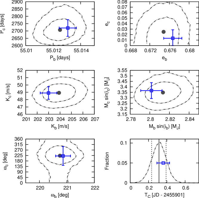
Figure 3.— Comparison between the Bayesian (MCMC) analysis and RVLIN$+$BOOTTRAN results. Top four and bottom left: Contours of the posterior distributions of selected orbital parameters ($P$, $e$, $K$, $M\sin{i}$, and $\omega$) based on the MCMC analysis (dashed dotted line). The $x$-axes are orbital parameters of the inner planet, $b$, and the $y$-axes are those of the outer planet, $c$. The inner contours mark the 68.27% (‘1$\sigma$’) 2-D confidence regions and the outer ones are 95.45% (‘2$\sigma$’) ones. Also plotted are the best Keplerian fit from RVLIN (blue squares) and $\pm$1$\sigma$ error bars estimated via bootstrapping (blue bars). Bottom right: Marginalized posterior distribution of time of conjunction (mid-transit) $T_{c}$ of HD 37605$b$ in dashed dotted line. The solid grey vertical line is the median of the distribution, and the dashed grey vertical lines mark 1$\sigma$ confidence interval. The blue square and its error bars are for the best estimate of $T_{c}$ from RVLIN$+$BOOTTRAN and its $\pm$1$\sigma$ errors. See § 3.3 for details. (A color version of this figure is available in the online journal.)

Table 3COMPARISON WITH MCMC RESULTS

Parameter	HD 37605$b$		HD 37605$c$
	RVLIN$+$BOOTTRAN	MCMC	RVLIN$+$BOOTTRAN	MCMC
$P$ (days)	55.01307 $\pm$ 0.00064	$55.01250\ {+0.00073}\ {-0.00075}$	2720 $\pm$ 57	$2707\ {+57}\ {-42}$
$T_{p}$ (BJD)	2453378.243 $\pm$ 0.020	$2453378.243\ {+0.025}\ {-0.024}$	2454838 $\pm$ 581	$2454838\ {+354}\ {-435}$
$T_{c}$ (BJD)	2455901.361 $\pm$ 0.069	$2455901.314\ {+0.077}\ {-0.081}$	$\cdots$	$\cdots$
$K$ (m s-1)	202.99 $\pm$ 0.72	$203.91\ {+0.92}\ {-0.88}$	48.90 $\pm$ 0.86	$48.93\ {+0.82}\ {-0.82}$
$e$	0.6767 $\pm$ 0.0019	$0.6748\ {+0.0022}\ {-0.0023}$	0.013 $\pm$ 0.015	$0.025\ {+0.022}\ {-0.017}$
$\omega$ (deg)	220.86 $\pm$ 0.28	$220.75\ {+0.33}\ {-0.32}$	221 $\pm$ 78	$223\ {+50}\ {-52}$
M (deg)	62.31 $\pm$ 0.15	$62.27\ {+0.18}\ {-0.18}$	117 $\pm$ 78	$118\ {+56}\ {-51}$
$M\sin{i}$ ($M_{\rm Jup}$)	2.802 $\pm$ 0.011	$2.814\ {+0.012}\ {-0.012}$	3.366 $\pm$ 0.072	$3.348\ {+0.065}\ {-0.062}$
$a$ (AU)	0.2831 $\pm$ 0.0016	$0.2833364\ {+0.0000027}\ {-0.0000027}$	3.814 $\pm$ 0.058	$3.809\ {+0.053}\ {-0.040}$
Jitter (m s-1)	3.6	$2.70\ {+0.53}\ {-0.46}$

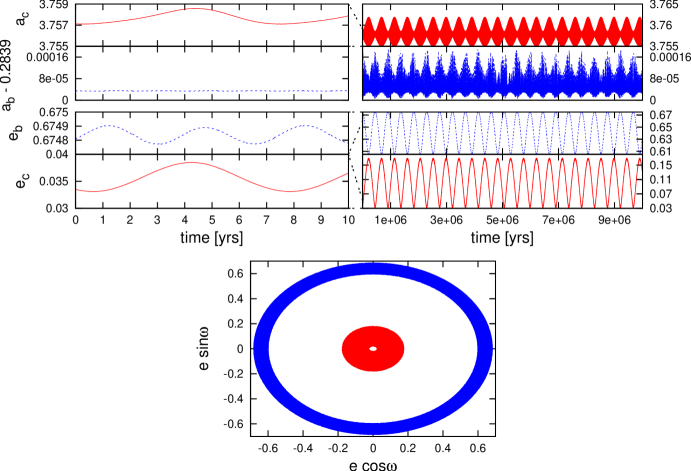
Figure 4.— Dynamic evolution of the best-fit MCMC system. On the left we plot the short-term evolution over 10 years, on the right we plot the evolution over $10^{7}$ years ($<1/10$ of our dynamic simulation time scale). The top plots describe the evolution of the semi-major axes and eccentricities of the inner planet ($a_{b}$ & $e_{b}$, blue dotted lines) and the outer planet ($a_{c}$ & $e_{c}$, red solid lines), while the bottom plot describes the parameter space covered by the $e\cos{\omega},e\sin{\omega}$ quantities over $10^{8}$ years (the blue and larger ring for inner planet, and the red and smaller ring for outer planet). We find that over the short-term (e.g., our RV observation window of $\sim 10$ years), the parameter variations are negligible, but in the long term significant eccentricity oscillations can take place (particularly noticeable in the eccentricity of the outer planet). See § 3.4 for details. (A color version of this figure is available in the online journal.)

3.3. Comparison with MCMC Results

We compared our best Keplerian fit from RVLIN and uncertainties derived from BOOTTRAN (abbreviated as RVLIN$+$BOOTTRAN hereafter) with that from a Bayesian framework following Ford (2005) and Ford (2006) (referred to as the MCMC analysis hereafter). Table 3 lists the major orbital parameters from both methods for a direct comparison. Fig. 3 illustrates this comparison, but with the MCMC results presented in terms of 2-D confidence contours for $P$, $e$, $K$, $M\sin{i}$, and $\omega$ of both planets, as well as for $T_{c}$ of HD 37605$b$.

For the Bayesian analysis, we assumed priors that are uniform in log of orbital period, eccentricity, argument of pericenter, mean anomaly at epoch, and the velocity zero-point. For the velocity amplitude ($K$) and jitter ($\sigma_{j}$), we adopted a prior of the form $p(x)=(x+x_{o})^{-1}[log(1+x/x_{o})]^{-1}$, with $K_{o}=\sigma_{j,o}=1$ m s^-1, i.e. high values are penalized. For a detailed discussion of priors, strategies to deal with correlated parameters, the choice of the proposal transition probability distribution function, and other details of the algorithm, we refer the reader to the original papers: Ford (2005, 2006); Ford & Gregory (2007). The likelihood for radial velocity terms assumes that each radial velocity observation ($v_{i}$) is independent and normally distributed about the true radial velocity with a variance of $\sigma_{i}^{2}+\sigma_{j}^{2}$, where $\sigma_{i}$ is the published measurement uncertainty. $\sigma_{j}$ is a jitter parameter that accounts for additional scatter due to stellar variability, instrumental errors and/or inaccuracies in the model (i.e., neglecting planet-planet interactions or additional, low amplitude planet signals).

We used an MCMC method based upon Keplerian orbits to calculate a sample from the posterior distribution (Ford, 2006). We calculated 5 Markov chains, each with $\sim 2\times 10^{8}$ states. We discarded the first half of the chains and calculate Gelman-Rubin test statistics for each model parameter and several ancillary variables. We found no indications of non-convergence amongst the individual chains. We randomly drew $3\times 10^{4}$ solutions from the second half of the Markov chains, creating a sample set of the converged overall posterior distribution of solutions. We then interrogated this sample on a parameter-by-parameter basis to find the median and $68.27\%\,(1$$\sigma)$ values reported in Table 3. We refer to this solution set below as the “best-fit” MCMC solutions.

We note that the periods of the two planets found in this system are very widely separated ($P_{c}/P_{b}\sim 50$), so we do not expect planet-planet interactions to be strong, hence we have chosen to forgo a numerically intensive N-body DEMCMC fitting procedure (see e.g. Johnson et al., 2011a; Payne & Ford, 2011) as the non-Keplerian perturbations should be tiny (detail on the magnitude of the perturbations is provided in §3.4). However, to ensure that the Keplerian fits generated are stable, we took the results of the Keplerian MCMC fits and injected those systems into the Mercury n-body package (Chambers, 1999) and integrated them forward for $\sim 10^{8}$ years. This allows us to verify that all of the selected best-fit systems from the Keplerian MCMC analysis are indeed long-term stable. Further details on the dynamical analysis of the system can be found in §3.4.

We assumed that all systems are coplanar and edge-on for the sake of this analysis, hence all of the masses used in our n-body analyses are minimum masses.

As shown in Table 3 and Fig. 3, the parameter estimates from RVLIN$+$BOOTTRAN and MCMC methods agree with each other very well (all within 1-$\sigma$ error bar). In some cases, the MCMC analysis reports error bars slightly larger than bootstrapping method ($\sim$ 20% at most). We note that the relatively large MCMC confidence intervals are not significantly reduced if one conducts an analysis at a fixed jitter level (e.g. $\sigma_{J}=3.5$m s^-1) unless one goes to an extremely low jitter value (e.g. $\sim 1.5$m s^-1). That is, the larger MCMC error bars do not simply result from treating the jitter as a free parameter. For the uncertainties on minimum planet mass $M\sin{i}$ and semi-major axes $a$, the MCMC analysis does not incorporate the errors on the stellar mass estimate. Note here, as previously mentioned in § 3.1, that the “best-fit” parameters reported by the MCMC analysis here listed in Table 3 are not a consistent set, as the best estimates were evaluated on a parameter-by-parameter basis, taking the median from marginalized posterior distribution of each. Assuming no jitter, The best Keplerian fit from RVLIN has a reduced chi-square value $\chi_{\nu}^{2}=2.28$, while the MCMC parameters listed in Table 3 give a higher $\chi_{\nu}^{2}$ value of 2.91.

3.4. Dynamical Analysis

We used the best-fit Keplerian MCMC parameters as the basis for a set of long-term numerical (n-body) integrations of the HD 37605 system using the Mercury integration package (Chambers, 1999). We used these integrations to verify that the best-fit systems: (i) are long-term stable; (ii) do not exhibit significant variations in their orbital elements on the timescale of the observations (justifying the assumption that the planet-planet interactions are negligible); (iii) do not exhibit any other unusual features. We emphasize again that the planets in this system are well separated and we do not expect any instability to occur: for the masses and eccentricities in question, a planet at $a_{b}\sim 0.28$ AU will have companion orbits which are Hill stable for $a\gtrsim 0.83$ AU (Gladman, 1993), so while Hill stability does not preclude outward scatter of the outer planet, the fact that $a_{c}\sim 3.8\gg 0.83$ AU suggests that the system will be far from any such instability.

We integrated the systems for $>10^{8}$ years ($\sim 10^{7}\times$ the orbital period of the outer planet and $>10^{2}\times$ the secular period of the system), and plot in Fig. 4 the evolution of the orbital elements $a,\ e$, & $\omega$. On the left-hand side of the plot we provide short-term detail, illustrating that over the $\sim 10$ year time period of our observations, the change in orbital elements will be very small. On the right-hand side we provide a much longer-term view, plotting $10^{7}$ out of $>10^{8}$ years of system evolution, demonstrating that (i) the secular variation in some of the elements (particularly the eccentricity of the outer planet; see $e_{c}$ in red) over a time span of $\sim 4\times 10^{5}$ years can be significant: in this case we see $0.03<e_{c}<0.11$, but (ii) the system appears completely stable, as one would expect for planets with a period ratio $P_{c}/P_{b}\sim 50$. Finally, at the bottom of the figure we display the range of parameter space covered by the $e_{i}\cos{\omega_{i}},\ e_{i}\sin{\omega_{i}}$ parameters ($i=b$ in blue for inner planet and $i=c$ in red for outer planet), demonstrating that the orbital alignments circulate, i.e. they do not show any signs of resonant confinement, which confirms our expectation of minimal planet-planet interaction as mentioned before.

As noted above, our analysis assumed coplanar planets. As such the planetary masses used in these dynamical simulations are minimum masses. We note that for inclined systems, the larger planetary masses will cause increased planet-planet perturbations. To demonstrate this is still likely to be unimportant, we performed a $10^{8}$ year simulation of a system in which $1/\sin{i}=10$, pushing the planetary masses to $\sim 30\ M_{\rm Jup}$. Even in such a pathological system the eccentricity oscillations are only increased by a factor of $\sim 2$ and the system remains completely stable for the duration of the simulation.

We also performed a separate Transit Timing Variation (TTV) analysis, using the best-fit MCMC systems as the basis for a set of highly detailed short-term integrations. From these we extracted the times of transit and found a TTV signal $\sim 100$ s, or $\sim 0.001$ day, which is much smaller than the error bar on $T_{c}$ ($\sim 0.07$ day). Therefore we did not take into account the effect of TTV when performing our transit analysis in the next section.

3.5. Activity Cycles and Jupiter Analogs

The coincidence of the Solar activity cycle period of 11 years and Jupiter’s orbital period near 12 years illustrates how activity cycles could, if they induced apparent line shifts in disk-integrated stellar spectra, confound attempts to detect Jupiter analogs around Sun-like stars. Indeed, Dravins (1985) predicted apparent radial velocity variations of up to 30 m s^-1 in solar lines due to the Solar cycle, and Deming et al. (1987) reported a tentative detection of such a signal in NIR CO lines of 30 m s^-1 in just 2 years, and noted that such an effect would severely hamper searches for Jupiter analogs. That concern was further amplified when Campbell et al. (1991) reported a positive correlation between radial velocity and chromospheric activity in the active star $\kappa^{1}$ Cet, with variations of order 50–100 m s^-1.

Wright et al. (2008) found that the star HD 154345 has an apparent Jupiter analog (HD 154345 $b$), but that this star also shows activity variations in phase with the radial velocity variations. They noted that many Sun-like stars, including the precise radial velocity standard star HD 185144 ($\sigma$ Dra) show similar activity variations and that rarely, if ever, are these signals well-correlated with signals similar in strength to that seen in HD 154345 ($\sim$ 15 m s^-1), and concluded that the similarity was therefore likely just an inevitable coincidence. Put succinctly, activity cycles in Sun-like stars are common (Baliunas et al., 1995), but few Jupiter analogs have been discovered, meaning that the early concern that activity cycles would mimic giant planets is not a severe problem.

Nonetheless, there is growing evidence that activity cycles can, in some stars, induce radial velocity variations (Santos et al., 2010; Lovis et al., 2011; Dumusque et al., 2012), and the example of HD 154345 still warrants care and concern. Most significantly, Dumusque et al. (2011) found a positive correlation between chromospheric activity and precise radial velocity in the average measurements of a sample of HARPS stars, and provided a formula for predicting the correlation strength as a function of the metallicity and effective temperature of the star. Their formulae predict a value of 2 m s^-1 for the most suspicious case in the literature, HD 154345 (compared to an actual semiamplitude of $\sim$ 15 m s^-1), but are rather uncertain. It is possible that in a few, rare cases, the formula might significantly underestimate the amplitude of the effect.

The top panel of Fig. 5 plots the T12 APT observations from all five observing seasons (data provided in Table 4; see details on APT photometry in § 4.1). The dashed line marks the mean relative magnitude ($\Delta(b+y)/2$) of the first season. The seasonal mean brightness of the star increases gradually from year to year by a total of $\sim 0.002$ mag, which may be due to a weak long-term magnetic cycle. However, no evidence is found in support of such a cycle in the Mount Wilson chromospheric Ca ii H & K indices (Isaacson & Fischer, 2010), although the S values vary by approximately 0.1 over the span of a few years. The formulae of Lovis et al. (2011) predict a corresponding RV variation of less than 2 m s^-1 due to activity, far too small to confound our planet detection with $K=49$ m s^-1.

Since we do not have activity measurements for this target over the span of the outer planet’s orbit in HD 37605, we cannot definitively rule out activity cycles as the origin of the effect, but the strength of the outer planetary signal and the lack of such signals in other stars known to cycle strongly dispels concerns that the longer signal is not planetary in origin.

4. The Dispositive Null Detection of Transits of HD 37605$b$

Figure 5.— Photometric observations of HD 37605 acquired over five years with the T12 0.8m APT. The top panel shows the entire five-year data set; the dotted line represents the mean brightness of the first observing season. A long-term brightening trend is evident with a total range in the seasonal means of 0.002 mag. The middle panel shows the photometric data normalized so that each season has the same mean as the first and then phased to the orbital period of HD 37605$b$ (55.01307 day). The solid line is the predicted transit light curve, with Phase 0.0 being the predicted time of mid-transit, $T_{c}$. A least-squares sine fit of the phased data produces the very small semi-amplitude of $0.00031~{}\pm~{}0.00011$ mag, providing strong evidence that the observed radial-velocity variations are not produced by rotational modulation of surface activity on the star. The bottom panel plots the observations near $T_{c}$ at an expanded scale on the abscissa. The horizontal bar below the transit window represents the $\pm$1$\sigma$ uncertainty in $T_{c}$. Unfortunately, none of the APT observations fall within the predicted transit window, so we are unable to rule out transits with the APT observations. See § 4.1 for more.

Figure 6.— Brightness variability in HD 37605 possibly induced by stellar rotation at $P=57.67\pm 0.30$ days. Top panel is the periodogram of the complete, normalized data set. Bottom panel shows the normalized photometry folded with this possible rotation period. The peak-to-peak amplitude is $0.00120~{}\pm~{}0.00021$ mag. See § 4.1 for more.

We have performed a transit search for the inner planet of the system, HD 37605$b$. This planet has a transit probability of 1.595% and a predicted transit duration of 0.352 day, as derived from the stellar parameters listed in Table 1 and the orbital parameters given in Table 2. From the minimum planet mass ($M\sin{i}=2.802\pm 0.011\ M_{\rm Jup}$; see Table 2) and the models of Bodenheimer et al. (2003), we estimate its radius to be $R_{\rm p}=1.1\ R_{\rm Jup}$. Combined with the stellar radius of HD 37605 listed in Table 1, $R_{\star}=0.901\pm 0.015\ R_{\odot}$, we estimate the transit depth to be 1.877% (for an edge-on transit, $i=90^{\circ}$). We used both ground-based (APT; §4.1) and space-based (MOST; §4.2) facilities in our search.

4.1. APT Observations and Analysis

The T12 0.8-m Automatic Photoelectric Telescope (APT), located at Fairborn Observatory in southern Arizona, acquired 696 photometric observations of HD 37605 between 2008 January 16 and 2012 April 7. Henry (1999) provides detailed descriptions of observing and data reduction procedures with the APTs at Fairborn. The measurements reported here are differential magnitudes in $\Delta(b+y)/2$, the mean of the differential magnitudes acquired simultaneously in the Strömgren $b$ and $y$ bands with two separate EMI 9124QB bi-alkali photomultiplier tubes. The differential magnitudes are computed from the mean of three comparison stars: HD 39374 (V = 6.90, B$-$V = 0.996, K0 III), HD 38145 (V = 7.89, B$-$V = 0.326, F0 V), and HD 38779 (V = 7.08, B$-$V = 0.413, F4 IV). This improves the precision of each individual measurement and helps to compensate for any real microvariability in the comp stars. Intercomparison of the differential magnitudes of these three comp stars demonstrates that all three are constant to 0.002 mag or better from night to night, consistent with typical single-measurement precision of the APT (0.0015-0.002 mag; Henry, 1999).

Table 4PHOTOMETRIC OBSERVATIONS OF HD 37605 FROM THE T12 0.8m APT

Heliocentric Julian Date	$\Delta(b+y)/2$
(HJD $-$ 2,400,000)	(mag)
54,481.7133	1.4454
54,482.6693	1.4474
54,482.7561	1.4442
54,483.6638	1.4452
54,495.7764	1.4469
54,498.7472	1.4470

Note. — This table is presented in its entirety in the electronic edition of the Astrophysical Journal. A portion is shown here for guidance regarding its form and content.

Fig. 5 illustrates the APT photometric data and our transit search. As mentioned in § 3.5, the top panel shows all of our APT photometry covering five observing seasons, which exhibits a small increasing trend in the stellar brightness. To search for the transit signal of HD 37605$b$, the photometric data were normalized so that all five seasons had the same mean (referred to as the “normalized photometry” hereafter). The data were then phased at the orbital period of HD 37605$b$, $55.01307$ days, and the predicted time of mid-transit, $T_{c}$, defined as Phase 0. The normalized and phased data are plotted in the middle panel of Fig. 5. The solid line is the predicted transit light curve, with the predicted transit duration (0.352 day or 0.0064 phase unit) and transit depth (1.877% or $\sim 0.020$ mag) as estimated above. The scatter of the phased data from their mean is $0.00197$ mag, consistent with APT’s single-measurement precision, and thus demonstrates that the combination of our photometric precision and the stability of HD 37605 is easily sufficient to detect the transits of HD 37605b in our phased data set covering five years. A least-squares sine fit of the phased data gives a very small semi-amplitude of $0.00031~{}\pm~{}0.00011$ mag (consistent with zero) and so provides strong evidence that the observed radial-velocity variations are not produced by rotational modulation of surface activity on the star.

The bottom panel of Fig. 5 plots the phased data around the predicted time of mid-transit, $T_{c}$, at an expanded scale on the abscissa. The horizontal bar below the transit window represents the $\pm$1$\sigma$ uncertainty on $T_{c}$ (0.138 day or 0.0025 phase unit for $T_{c}$’s near BJD $2,455,901.361$; see § 3.2). The light curve appears to be highly clustered, or binned, due to the near integral orbital period ($P\sim 55.01$ days) and consequent incomplete sampling from a single observing site. Unfortunately, none of the data clusters chance to fall within the predicted transit window, so we are unable to rule out transits of HD 37605b with the APT observations.

Periodogram analysis of the five individual observing seasons revealed no significant periodicity between 1 and 100 days. This suggests that the star is inactive and the observed $K\sim 200$ m s^-1 RV signal (for HD 37605$b$) is unlikely to be the result of stellar activity.

Analysis of the complete, normalized data set, however, suggests a week periodicity of $57.67\pm 0.30$ days with a peak-to-peak amplitude of just $0.0012\pm 0.0002$ mag (see Fig. 6). We tentatively identify this as the stellar rotation period. This period is consistent with the projected rotational velocity of $v\sin{i}<1$ km s^-1derived from our stellar analysis described in §2.3. It is also consistent with the analysis of Isaacson & Fischer (2010), who derived a Mount Wilson chromospheric Ca ii H & K index of $S=0.165$, corresponding to $\log R^{\prime}_{\rm HK}=-5.03$. Together, these results imply a rotation period $\gtrsim 46$ days and an age of $\sim 7$ Gyr (see Table 1). Similarly, Ibukiyama & Arimoto (2002) find an age of $>10$ Gyr using isochrones along with the Hipparcos parallax and space motion, supporting HD 37605’s low activity and long rotation period.

4.2. MOST Observations and Analysis

Figure 7.— Photometric observations of HD 37605 by the MOST satellite, which rule out the edge-on transit of HD 37605$b$ at a $\gg$ 10$\sigma$ level. The solid line is the predicted transit light curve, and the dashed vertical lines are the 1$\sigma$ transit window boundaries defined by adding $\sigma_{T_{c}}$ (0.069 day) on both sides of the predicted transit window (0.352-day wide). See § 4.2 for more details.

Table 5PHOTOMETRIC OBSERVATIONS OF HD 37605 ON MOST

Heliocentric Julian Date	Relative Magnitude
(HJD $-$ 2,451,545)	(mag)
4355.5105	-0.0032
4355.5112	-0.0047
4355.5119	-0.0018
4355.5126	-0.0026
4355.5133	-0.0018
4355.5140	-0.0039

Note. — This table is presented in its entirety in the electronic edition of the Astrophysical Journal. A portion is shown here for guidance regarding its form and content.

As noted earlier, the near-integer period of HD 37605$b$ makes it difficult to observe from a single longitude. The brightness of the target and the relatively long predicted transit duration creates additional challenges for ground-based observations. We thus observed HD 37605 during 2011 December 5–6 (around the predicted $T_{c}$ at BJD $2,455,901.361$ as listed in Table 2) with the MOST (Microvariability and Oscillations of Stars) satellite launched in 2003 (Walker et al., 2003; Matthews et al., 2004) in the Direct Imaging mode. This observing technique is similar to ground-based CCD photometry, allowing to apply traditional aperture and PSF procedures for data extraction (see e.g. Rowe et al., 2006, for details). Outlying data points caused by, e.g., cosmic rays were removed.

MOST is orbiting with a period of $\sim$ 101 minutes (14.19 cycles per day, cd^-1), which leads to a periodic artifact induced by the scattered light from the earthshine. This signal and its harmonics are further modulated with a frequency of 1 cd^-1 originating from the changing albedo of the earth. To correct for this phenomenon, we constructed a cubic fit between the mean background and the stellar flux, which was then subtracted from the data. The reduced and calibrated MOST photometric data are listed in Table 5.

The MOST photometry is shown in Figure 7 for the transit window observations. The vertical dashed lines indicate the beginning and end of the 1 $\sigma$ transit window defined by adding $\sigma_{T_{c}}$ (0.069 day) on both sides of the predicted transit duration of 0.352 days. The solid line shows the predicted transit model for the previously described planetary parameters. The mean of the relative photometry is 0.00% (or 0.00 mag), with a rms scatter of 0.17%, and within the predicted transit window there are 58 MOST observations. Therefore, the standard error on the mean relative photometry is 0.17%$/\sqrt{58}=$ 0.022%. This means that, for the predicted transit window and a predicted depth of 1.877%, we can conclude a null detection of HD 37605$b$’s transit with extremely high confidence (149$\sigma$).

Note that the above significance is for an edge-on transit with an impact parameter of $b=0.0$. A planetary trajectory across the stellar disk with a higher impact parameter will produce a shorter transit duration. However, the gap between each cluster of MOST measurements is 0.06 days which is 17% of the edge-on transit duration. In order for the duration to be fit within the data gaps, the impact parameter would need to be $b>0.996$. To estimate a more conservative lower limit for $b$, we now assume the most unfortunate case where the transit center falls exactly in the middle of one of the measurement gaps, and also consider the effect of limb darkening by using the non-linear limb darkening model by Mandel & Agol (2002) with their fitted coefficients for HD 209458. Even under this scenario, we can still conclude the null detection for any transit with $b<0.951$ at $\gtrsim 5\sigma$ (taking into account that there are at least $\sim$ 20 observations will fall within the transit window in this case, though only catching the shallower parts of the transit light curve).

All of the above is based on the assumption that the planet has the predicted radius of 1.1 $R_{\rm Jup}$. If in reality the planet is so small that even a $b=0$ transit would fall below our detection threshold, it would mean that the planet has a radius of $<0.36\ R_{\rm Jup}$ (a density of $>$ 74.50 g$/$cm³), which seems unlikely. It is also very unlikely that our MOST photometry has missed the transit window completely due to an ill-predicted $T_{c}$. In the sampling distribution of $T_{c}$ from BOOTTRAN (with 1000 replicates; see § 3.2 and Appendix), there is no $T_{c}$ that would put the transit window completely off the MOST coverage. In the marginalized posterior distribution of $T_{c}$ calculated via MCMC (see § 3.3 and Fig. 3), there is only 1 such $T_{c}$ out of $3\times 10^{4}$ (0.003%).

5. Summary and Conclusion

In this paper, we report the discovery of HD 37605$c$ and the dispositive null detection of non-grazing transits of HD 37605$b$, the first planet discovered by HET. HD 37605$c$ is the outer planet of the system with a period of $\sim 7.5$ years on a nearly circular orbit ($e=0.013$) at $a=3.814$ AU. It is a “Jupiter analog” with $M\sin{i}=3.366\ M_{\rm Jup}$, which adds one more sample to the currently still small inventory of such planets (only 10 including HD 37605$c$; see §1). The discovery and characterization of “Jupiter analogs” will help understanding the formation of gas giants as well as the frequency of true solar system analogs. This discovery is a testimony to the power of continued observation of planet-bearing stars.

Using our RV data with nearly 8-year long baseline, we refined the orbital parameters and transit ephemerides of HD 37605$b$. The uncertainty on the predicted mid-transit time was constrained down to 0.069 day (at and near $T_{c}=2,455,901.361$ in BJD), which is small compared to the transit duration (0.352 day). In fact, just the inclusion of the two most recent points in our RV data have reduced the uncertainty on $T_{c}$ by over 10%. We have performed transit search with APT and the MOST satellite. Because of the near-integer period of HD 37605$b$ and the longitude of Fairborn Observatory, the APT photometry was unable to cover the transit window. However, its excellent photometric precision over five observing seasons enabled us to rule out the possibility of the RV signal being induced by stellar activity. The MOST photometric data, on the other hand, were able to rule out an edge-on transit with a predicted depth of 1.877% at a $\gg$ 10$\sigma$ level, with a $5\sigma$ lower limit on the impact parameter of $b\leq 0.951$. This transit exclusion is a further demonstration of the TERMS strategy, where follow-up RV observations help to reduce the uncertainty on transit timing and enable transit searches.

Our best-fit orbital parameters and errors from RVLIN$+$BOOTTRAN were found to be consistent with those derived from a Bayesian analysis using MCMC. Based on the best-fit MCMC systems, we performed dynamic and TTV analysis on the HD 37605 system. Dynamic analysis shows no sign of orbital resonance and very minimal planet-planet interaction. We derived a TTV of $\sim$100 s, which is much smaller than $\sigma_{T_{c}}$.

We have also performed a stellar analysis on HD 37605, which shows that it is a metal rich star ($[{\rm Fe/H}]=0.336\pm 0.030$) with a stellar mass of $M_{\star}=1.000\pm 0.017\ M_{\odot}$ with a radius of $R_{\star}=0.901\pm 0.015$. The small variation seen in our photometric data (amplitude $<0.003$ mag over the course of four years) suggests that HD 37605 is consistent as being an old, inactive star that is probably slowly rotating. We tentatively propose that the rotation period of the star is $57.67\pm 0.30$ days, based on a weak periodic signal seen in our APT photometry.

6. Note on Previously Published Orbital Fits

In early 2012, we repaired a minor bug in the BOOTTRAN package, mostly involving the calculation and error bar estimation of $M\sin{i}$. As a result, the $M\sin{i}$ values and their errors for two previously published systems (three planets) need to be updated. They are: HD 114762$b$ (Kane et al., 2011a), HD 168443$b$, and HD 168443$c$ (Pilyavsky et al., 2011b). Table 6 lists the updated $M\sin{i}$ and error bars.

One additional system, HD 63454 (Kane et al., 2011d), was also analyzed using BOOTTRAN. However, the mass of HD 63454$b$ is small enough compared to its host mass and thus was not affected by this change.

Table 6Updated $M\sin{i}$ and Errors for HD 114762$b$ and HD 168443$b$, $c$

Planet	$M\sin{i}~{}\pm$ std. error ($M_{\rm Jup}$)
HD 114762$b$	$11.086\pm 0.067$
HD 114762$b$	$11.069\pm 0.063$
HD 168443$b$	$7.696\pm 0.015$
HD 168443$c$	$17.378\pm 0.044$

Uncertainties via Bootstrapping

The uncertainties listed for the orbital parameter estimates and transit mid-time $T_{c}$ are calculated via bootstrapping (Freedman, 1981; Davison & Hinkley, 1997) using the package BOOTTRAN, which we have made publicly available (see § 3.2). It is designed to calculate error bars for transit ephemerides and the Keplerian orbital fit parameters output by the RVLIN package(Wright & Howard, 2009), but can also be a stand-alone package. Thanks to the simple concept of bootstrapping, it is computationally very time-efficient and easy to use.

The basic idea of bootstrap is to resample based on original data to create bootstrap samples (multiple data replicates); then for each bootstrap sample, derive orbital parameters or transit parameters through orbital fitting and calculation. The ensemble of parameters obtained in this way yields the approximate sampling distribution for each estimated parameter. The standard deviation of this sampling distribution is the standard error for the estimate.

We caution the readers here that there are regimes in which the “approximate sampling distribution” (a frequentist’s concept) is not an estimate of the posterior probability distribution (a Bayesian concept), and there are regimes (e.g., when limited sampling affects the shape of the $\chi^{2}$ surface) where there are qualitative differences and the bootstrap method dramatically underestimates uncertainties (e.g., long-period planets when the observations are not yet sufficient to pin down the orbital period; Ford, 2005; Bender et al., 2012). In situations with sufficient RV data, good phase coverage, a sufficient time span of observations and a good orbital fit, bootstrap often gives a useful estimate of the parameter uncertainties. For the data considered in this paper, it was not obvious that the bootstrap uncertainty estimate would be accurate, as the time span of observations is only slightly longer than the orbital period of planet $c$. Nevertheless, we find good agreement between the uncertainty estimates derived from bootstrap and MCMC calculations.

The radial velocity data are denoted as $\{\vec{t},\ \vec{v},\ \vec{\sigma}\}$, where each $t_{i}$, $v_{i}$, $\sigma_{i}$ represents radial velocity $v_{i}$ observed at time (BJD) $t_{i}$ with velocity uncertainty $\sigma_{i}$. Extreme outliers should be rejected in order to preserve the validity of our bootstrap algorithm. We first derive our estimates for the true orbital parameters from the original RV data via orbital fitting, using the RVLIN package (Wright & Howard, 2009):

$$\vec{\beta}=\mu(\vec{t},\ \vec{v},\ \vec{\sigma}),$$ (1)

where $\vec{\beta}$ is the best fitted orbital parameters. From $\vec{\beta}$, we derive $\{\vec{t},\ \vec{v}_{best}(\vec{\beta})\}$, the best-fit model (here $\vec{t}$ are treated as predictors and thus fixed). Then we can begin resampling to create bootstrap samples.

Our resampling plan is model-based resampling, where we draw from the residuals against the best-fit model. For data that come from the same instrument or telescope, in which case no instrumental offset needs to be taken into account, we simply draw from all residuals, $\{\vec{v}-\vec{v}_{best}\}$, with equal probability for each $(v_{i}-v_{best,i})$. This new ensemble of residuals, denoted as ${\vec{r^{*}}}$, is then added to the best-fit model $\vec{v}_{best}$ to create one bootstrap sample, $\vec{v^{*}}$ . Associated with ${\vec{r^{*}}}$, the uncertainties $\vec{\sigma}$ are also re-assigned to $\vec{v^{*}}$ – that is, if $v_{j}-v_{best,j}$ is drawn as $r_{k}$ and added to $v_{k}$ to generate $v^{*}_{k}$, then the uncertainty for $v^{*}_{k}$ is set to be $\sigma_{j}$.

For data that come from multiple instruments or multiple telescopes, we incorporate our model-based resampling plan to include stratified sampling. In this case, although data from each instrument or telescope are close to homoscedastic, the entire set of data are usually highly heteroscedastic due to stratification in instrument/telescope radial velocity precision. Therefore, the resampling process is done by breaking down the data into different groups, $\{\vec{v_{1}},\ \vec{v_{2}},\ \ldots\}$, according to instrument and/or telescope, and then resample within each subgroup of data with the algorithm described in last paragraph. The bootstrap sample is then $\vec{v^{*}}=\{\vec{v^{*}}_{1},\ \vec{v^{*}}_{2},\ \ldots\}$.

To construct the approximate sampling distribution of the orbital parameter estimates $\vec{\beta}$, we compute

$$\vec{\beta^{*}}=\mu(\vec{t},\ \vec{v^{*}},\ \vec{\sigma^{*}})$$ (2)

for each bootstrap sample, $\{\vec{t},\ \vec{v^{*}},\ \vec{\sigma^{*}}\}$. The sampling distribution for each orbital parameter estimate $\beta_{i}$ can be constructed from the multiple sets of $\vec{\beta^{*}}$ calculated from multiple bootstrap samples ($\vec{\beta^{*}}^{(1)},\ \vec{\beta^{*}}^{(2)},\ \ldots$ from $\vec{v^{*}}^{(1)},\ \vec{v^{*}}^{(2)},\ \ldots$). The standard errors for $\vec{\beta}$ are simply the standard deviations of the sampling distributions.

The sampling distribution of the estimated transit mid-time, $T_{c}$, is calculated likewise. Here $T_{c}$ is the transit time for a certain planet of interest in the system, and is usually specified to be the first transit after a designated time $T$. However, the situation is complicated by the periodic nature of $T_{c}$. Our approach is to first calculate, based on the original RV data, $T_{c0}$, the estimated mid-time of the first transit after time $T_{0}$ (an arbitrary time within the RV observation time window of $[\min(\vec{t}),\ \max(\vec{t})]$; $T_{c0}$ is also within this window). Then

$$T_{c}=N\cdot P+T_{c0},$$ (3)

where $P$ is the best-estimated period for this planet of interest, and $N$ is the smallest integer that is larger than $(T-T_{c0})/P$. Next we compute $T_{c0}^{*}$ for each bootstrap sample $\{\vec{t},\ \vec{v^{*}},\ \vec{\sigma^{*}}\}$. Given that within the time window of radial velocity observations ($[\min(\vec{t}),\ \max(\vec{t})]$), the phase of the planet should be known well enough, it is fair to assume that $T_{c0}$ is an unbiased estimator of the true transit mid-time. Therefore we assert that $T_{c0}^{*}$ has to be well constrained and within the range of $[T_{c0}-P^{*}/2,\ T_{c0}+P^{*}/2]$, where $P^{*}$ is the period estimated from this bootstrap sample. If not, then we subtract or add multiple $P^{*}$’s until $T_{c0}^{*}$ falls within the range. Then naturally

$$T_{c}^{*}=N\cdot P^{*}+T_{c0}^{*}.$$ (4)

The ensemble of $T_{c}^{*}$’s gives the sampling distribution of $T_{c}$ and its standard error. Note that $T_{c}^{*}$ is not necessarily within the rage of $[T_{c}-P/2,\ T_{c}+P/2]$.

Provided with the stellar mass $M_{\star}$ and its uncertainty, we calculate, for each planet in the system, the standard errors for the semi-major axis $a$ and the minimum mass of the planet $M_{\rm p,min}$ (denoted as $M\sin{i}$ in the main text as commonly seen in literature, but this is a somewhat imprecise notation). As the first step, the mass function is calculated for the best-fit $\vec{\beta}$ and each bootstrap sample $\vec{\beta^{*}}$,

$$f(P,K,e)=\frac{PK^{3}(1-e)^{3/2}}{2\pi G}=\frac{(M_{p}\cdot\sin i)^{3}}{(M_{\star}+M_{p})^{2}}.$$ (5)

The sampling distribution of $f(P,K,e)$ then gives the standard error of the mass function. The minimum mass of the planet $M_{\rm p,min}$ is then calculated by assuming $\sin{i}=1$ and solving for $M_{p}$. Standard error of $M_{\rm p,min}$ is derived through simple propagation of error, as the covariance between $M_{\star}$ and $f(P,K,e)$ is probably negligible.

For the semi-major axis $a$,

$$a^{3}=\frac{P^{2}G(M_{\star}+M_{p})}{4\pi^{2}}\approx\frac{P^{2}G(M_{\star}+M_{\rm p,min})}{4\pi^{2}}.$$ (6)

The standard error of $P^{2}$ is calculated from its bootstrap sampling distribution, and via simple propagation of error we obtain the standard error of $a$ (neglecting covariance between $P^{2}$, $M_{\rm p,min}$, and $M_{\star}$).

Table 7HET and KECK RADIAL VELOCITIES FOR HD 37605

	Velocity	Uncertainty
BJD$-2440000\ \$	(m s-1)	(m s-1)	Telescope
13002.671503	122.4	8.8	HET
13003.685247	126.9	5.6	HET
13006.662040	132.1	5.2	HET
13008.664059	130.4	4.8	HET
13010.804767	113.4	4.7	HET
13013.793987	106.2	4.9	HET
13042.727963	-120.0	4.7	HET
13061.667551	126.5	4.0	HET
13065.646834	111.3	5.8	HET
13071.643820	106.7	5.5	HET
13073.638180	91.7	4.6	HET
13082.623709	53.4	5.7	HET
13083.595357	45.1	6.4	HET
13088.593775	30.7	11.3	HET
13089.595750	0.8	5.5	HET
13092.597983	-25.5	6.2	HET
13094.586570	-51.0	5.9	HET
13095.586413	-72.2	6.2	HET
13096.587432	-75.0	9.3	HET
13098.576213	-173.1	6.4	HET
13264.951365	-194.0	9.8	HET
13265.947438	-238.2	10.5	HET
13266.945977	-264.2	13.1	HET
13266.959470	-286.8	11.6	HET
13283.922407	118.8	9.6	HET
13318.819260	-142.8	6.6	HET
13335.921770	143.4	6.3	HET
13338.906008	132.1	5.4	HET
13377.819405	-279.6	6.1	HET
13378.811880	-161.3	5.2	HET
13379.802247	-39.7	5.2	HET
13381.644284	74.4	4.7	HET
13384.646538	112.5	5.8	HET
13724.855831	88.1	5.3	HET
13731.697227	57.8	5.0	HET
13738.674709	36.4	4.9	HET
13743.810196	14.1	5.7	HET
13748.647234	-17.8	5.6	HET
14039.850147	-104.1	5.5	HET
14054.964568	68.8	7.3	HET
14055.952778	49.3	6.5	HET
14067.762810	22.1	6.0	HET
14374.924086	32.7	8.6	HET
14394.864468	-12.1	8.5	HET
14440.883298	11.9	8.5	HET
14467.826532	-121.9	6.3	HET
14487.613032	40.4	5.6	HET
14515.689341	-55.6	5.7	HET
14550.600301	23.1	5.5	HET
14759.878895	34.3	4.9	HET
14776.839187	2.0	6.7	HET
14787.793398	-40.8	5.1	HET
14907.617522	-94.4	5.1	HET
15089.968860	76.4	4.1	HET
15104.917965	54.0	4.6	HET
15123.882222	-44.4	4.6	HET
15172.734743	-0.4	4.6	HET
15172.749345	3.0	4.9	HET
15180.715307	-65.0	5.3	HET
15190.692697	-257.0	4.9	HET
15190.704818	-252.3	6.3	HET
15195.678923	-47.7	5.1	HET
15200.809909	85.1	4.5	HET
15206.665616	75.9	4.5	HET
15208.646672	72.6	5.7	HET
15266.634586	81.1	4.6	HET
15274.598361	57.1	4.6	HET
15280.605398	24.3	5.6	HET
15450.974863	25.2	5.2	HET
15469.928975	-81.7	4.4	HET
15481.884352	110.8	4.8	HET
15494.004309	71.2	4.9	HET
15500.853302	41.1	6.0	HET
15505.824457	21.2	4.8	HET
15510.809500	-13.9	5.5	HET
15511.813809	-18.4	4.7	HET
15518.798148	-139.1	4.9	HET
15518.943518	-148.8	4.6	HET
15524.791579	-97.7	6.0	HET
15526.759230	51.2	5.8	HET
15526.767959	56.5	6.1	HET
15527.921902	89.2	4.6	HET
15528.921753	105.1	5.5	HET
15530.757847	120.6	5.3	HET
15532.760658	117.6	4.8	HET
15544.730827	81.8	4.9	HET
15545.871710	87.7	5.2	HET
15547.717980	78.6	6.5	HET
15547.720596	81.2	7.8	HET
15550.703130	75.8	5.5	HET
15556.688398	43.4	5.0	HET
15557.842853	40.1	4.9	HET
15566.657803	-18.4	5.6	HET
15566.666973	-19.0	4.9	HET
15569.670948	-50.7	4.5	HET
15571.659560	-94.0	7.4	HET
15571.662188	-99.5	7.5	HET
15582.777052	75.1	5.4	HET
13982.116400	-312.6	1.1	Keck
13983.110185	-291.6	1.1	Keck
13984.104595	-175.0	1.1	Keck
14024.076794	-39.9	1.2	Keck
14129.848461	-17.1	1.1	Keck
14131.926354	-32.2	1.3	Keck
14138.913472	-98.8	1.2	Keck
14544.815162	54.2	1.0	Keck
14545.799155	50.4	1.0	Keck
14546.802812	48.1	1.0	Keck
15172.939733	21.7	1.1	Keck
15435.133695	97.5	1.0	Keck
15521.851677	-244.2	1.2	Keck
15522.947381	-268.1	1.1	Keck
15526.936103	78.6	1.1	Keck
15528.877669	118.4	1.0	Keck
15543.032113	115.5	1.2	Keck
15545.105481	110.3	1.2	Keck
15546.046328	110.6	1.2	Keck
15556.071287	69.6	1.1	Keck
15556.954989	66.4	1.1	Keck
15558.027806	62.3	1.2	Keck
15584.769501	128.2	1.2	Keck
15606.952224	91.6	1.2	Keck
15634.789262	-81.0	1.0	Keck
15636.793990	80.7	1.0	Keck
15636.799360	85.6	1.1	Keck
15663.738831	87.6	1.0	Keck
15671.731754	45.8	1.2	Keck
15672.732058	37.1	1.0	Keck
15673.745070	27.6	1.0	Keck
15793.124325	-86.7	1.2	Keck
15843.017282	-6.4	1.3	Keck

References

- Bailey et al. (2009) Bailey, J., Butler, R. P., Tinney, C. G., Jones, H. R. A., O’Toole, S., Carter, B. D., & Marcy, G. W. 2009, ApJ, 690, 743
- Baliunas et al. (1995) Baliunas, S. L., et al. 1995, ApJ, 438, 269
- Baluev (2009) Baluev, R. V. 2009, MNRAS, 393, 969
- Barbieri et al. (2007) Barbieri, M., et al. 2007, A&A, 476, L13
- Bender et al. (2012) Bender, C. F., et al. 2012, ApJ, 751, L31
- Bodenheimer et al. (2003) Bodenheimer, P., Laughlin, G., & Lin, D. N. C. 2003, ApJ, 592, 555
- Boisse et al. (2012) Boisse, I., et al. 2012, A&A, 545, A55
- Bouchy et al. (2005) Bouchy, F., et al. 2005, A&A, 444, L15
- Butler et al. (1996) Butler, R. P., Marcy, G. W., Williams, E., McCarthy, C., Dosanjh, P., & Vogt, S. S. 1996, PASP, 108, 500
- Campbell et al. (1991) Campbell, B., Yang, S., Irwin, A. W., & Walker, G. A. H. 1991, in Lecture Notes in Physics, Berlin Springer Verlag, Vol. 390, Bioastronomy: The Search for Extraterrestial Life — The Exploration Broadens, ed. J. Heidmann & M. J. Klein, 19–20
- Chambers (1999) Chambers, J. E. 1999, MNRAS, 304, 793
- Charbonneau et al. (2000) Charbonneau, D., Brown, T. M., Latham, D. W., & Mayor, M. 2000, ApJ, 529, L45
- Cochran et al. (2004) Cochran, W. D., et al. 2004, ApJ, 611, L133
- Davison & Hinkley (1997) Davison, A., & Hinkley, D. 1997, Bootstrap Methods and Their Application, Cambridge Series on Statistical and Probabilistic Mathematics (Cambridge University Press)
- Demarque et al. (2004) Demarque, P., Woo, J.-H., Kim, Y.-C., & Yi, S. K. 2004, ApJS, 155, 667
- Deming et al. (1987) Deming, D., Espenak, F., Jennings, D. E., Brault, J. W., & Wagner, J. 1987, ApJ, 316, 771
- Demory et al. (2011) Demory, B.-O., et al. 2011, A&A, 533, A114
- Dragomir et al. (2011) Dragomir, D., et al. 2011, AJ, 142, 115
- Dravins (1985) Dravins, D. 1985, in Stellar Radial Velocities, ed. A. G. D. Philip & D. W. Latham, 311–320
- Dumusque et al. (2011) Dumusque, X., et al. 2011, A&A, 535, A55
- Dumusque et al. (2012) —. 2012, Nature, advanced online publication, doi:10.1038/nature11572
- ESA (1997) ESA. 1997, VizieR Online Data Catalog, 1239, 0
- Fischer et al. (2007) Fischer, D. A., et al. 2007, ApJ, 669, 1336
- Ford (2005) Ford, E. B. 2005, AJ, 129, 1706
- Ford (2006) —. 2006, ApJ, 642, 505
- Ford & Gregory (2007) Ford, E. B., & Gregory, P. C. 2007, in Astronomical Society of the Pacific Conference Series, Vol. 371, Statistical Challenges in Modern Astronomy IV, ed. G. J. Babu & E. D. Feigelson, 189
- Fossey et al. (2009) Fossey, S. J., Waldmann, I. P., & Kipping, D. M. 2009, MNRAS, 396, L16
- Freedman (1981) Freedman, D. A. 1981, The Annals of Statistics, 9, pp. 1218
- Gladman (1993) Gladman, B. 1993, Icarus, 106, 247
- Henry (1999) Henry, G. W. 1999, PASP, 111, 845
- Henry et al. (2000) Henry, G. W., Marcy, G. W., Butler, R. P., & Vogt, S. S. 2000, ApJ, 529, L41
- Hoaglin et al. (1983) Hoaglin, D. C., Mosteller, F., & Tukey, J. W. 1983, Understanding Robust and Exploratory Data Anlysis, Wiley Classics Library Editions (Wiley)
- Horne (1986) Horne, K. 1986, PASP, 98, 609
- Howard et al. (2009) Howard, A. W., et al. 2009, ApJ, 696, 75
- Howard et al. (2010) —. 2010, ApJ, 721, 1467
- Howard et al. (2011) —. 2011, ApJ, 726, 73
- Ibukiyama & Arimoto (2002) Ibukiyama, A., & Arimoto, N. 2002, A&A, 394, 927
- Isaacson & Fischer (2010) Isaacson, H., & Fischer, D. 2010, ApJ, 725, 875
- Johnson et al. (2011a) Johnson, J. A., et al. 2011a, AJ, 141, 16
- Johnson et al. (2011b) —. 2011b, ApJS, 197, 26
- Jones et al. (2010) Jones, H. R. A., et al. 2010, MNRAS, 403, 1703
- Kane et al. (2012) Kane, S. R., Ephemeris Refinement, T., & Survey(TERMS), M. 2012, in American Astronomical Society Meeting Abstracts, Vol. 219, American Astronomical Society Meeting Abstracts, #228.07
- Kane et al. (2011a) Kane, S. R., Henry, G. W., Dragomir, D., Fischer, D. A., Howard, A. W., Wang, X., & Wright, J. T. 2011a, ApJ, 735, L41
- Kane et al. (2009) Kane, S. R., Mahadevan, S., von Braun, K., Laughlin, G., & Ciardi, D. R. 2009, PASP, 121, 1386
- Kane et al. (2011b) Kane, S. R., et al. 2011b, Detection and Dynamics of Transiting Exoplanets, St. Michel l’Observatoire, France, Edited by F. Bouchy; R. Díaz; C. Moutou; EPJ Web of Conferences, Volume 11, id.06005, 11, 6005
- Kane et al. (2011c) Kane, S. R., et al. 2011c, in American Astronomical Society Meeting Abstracts, #128.03
- Kane et al. (2011d) —. 2011d, ApJ, 737, 58
- Laughlin et al. (2009) Laughlin, G., Deming, D., Langton, J., Kasen, D., Vogt, S., Butler, P., Rivera, E., & Meschiari, S. 2009, Nature, 457, 562
- Lovis et al. (2011) Lovis, C., et al. 2011, A&A submitted
- Mandel & Agol (2002) Mandel, K., & Agol, E. 2002, ApJ, 580, L171
- Marcy & Butler (1992) Marcy, G. W., & Butler, R. P. 1992, PASP, 104, 270
- Marcy et al. (2002) Marcy, G. W., Butler, R. P., Fischer, D. A., Laughlin, G., Vogt, S. S., Henry, G. W., & Pourbaix, D. 2002, ApJ, 581, 1375
- Matthews et al. (2004) Matthews, J. M., Kuschnig, R., Guenther, D. B., Walker, G. A. H., Moffat, A. F. J., Rucinski, S. M., Sasselov, D., & Weiss, W. W. 2004, Nature, 430, 51
- McArthur et al. (2004) McArthur, B. E., et al. 2004, ApJ, 614, L81
- Michelson & Morley (1887) Michelson, A. A., & Morley, E. 1887, American Journal of Science, 34, 333
- Moutou et al. (2011) Moutou, C., et al. 2011, A&A, 527, A63
- Payne & Ford (2011) Payne, M. J., & Ford, E. B. 2011, ApJ, 729, 98
- Pepe et al. (2007) Pepe, F., et al. 2007, A&A, 462, 769
- Pilyavsky et al. (2011a) Pilyavsky, G., et al. 2011a, ApJ, 743, 162
- Pilyavsky et al. (2011b) —. 2011b, ApJ, 743, 162
- Piskunov & Valenti (2002) Piskunov, N. E., & Valenti, J. A. 2002, A&A, 385, 1095
- Rowe et al. (2006) Rowe, J. F., et al. 2006, ApJ, 646, 1241
- Santos et al. (2010) Santos, N. C., Gomes da Silva, J., Lovis, C., & Melo, C. 2010, A&A, 511, A54
- Santos et al. (2005) Santos, N. C., Israelian, G., Mayor, M., Bento, J. P., Almeida, P. C., Sousa, S. G., & Ecuvillon, A. 2005, A&A, 437, 1127
- Schneider et al. (2011) Schneider, J., Dedieu, C., Le Sidaner, P., Savalle, R., & Zolotukhin, I. 2011, A&A, 532, A79
- Shetrone et al. (2007) Shetrone, M., et al. 2007, PASP, 119, 556
- Torres et al. (2010) Torres, G., Andersen, J., & Giménez, A. 2010, A&A Rev., 18, 67
- Tull (1998) Tull, R. G. 1998, in Society of Photo-Optical Instrumentation Engineers (SPIE) Conference Series, Vol. 3355, Society of Photo-Optical Instrumentation Engineers (SPIE) Conference Series, ed. S. D’Odorico, 387–398
- Valenti & Fischer (2005) Valenti, J. A., & Fischer, D. A. 2005, ApJS, 159, 141
- Valenti & Piskunov (1996) Valenti, J. A., & Piskunov, N. 1996, A&AS, 118, 595
- Valenti et al. (2009) Valenti, J. A., et al. 2009, 702, 989
- van Leeuwen (2008) van Leeuwen, F. 2008, VizieR Online Data Catalog, 1311, 0
- Vogt et al. (1994) Vogt, S. S., et al. 1994, in Society of Photo-Optical Instrumentation Engineers (SPIE) Conference Series, Vol. 2198, Society of Photo-Optical Instrumentation Engineers (SPIE) Conference Series, ed. D. L. Crawford & E. R. Craine, 362
- Walker et al. (2003) Walker, G., et al. 2003, PASP, 115, 1023
- Wittenmyer et al. (2007) Wittenmyer, R. A., Endl, M., Cochran, W. D., & Levison, H. F. 2007, AJ, 134, 1276
- Wittenmyer et al. (2012) Wittenmyer, R. A., et al. 2012, ApJ, 753, 169
- Wright & Howard (2009) Wright, J. T., & Howard, A. W. 2009, ApJS, 182, 205
- Wright et al. (2008) Wright, J. T., Marcy, G. W., Butler, R. P., Vogt, S. S., Henry, G. W., Isaacson, H., & Howard, A. W. 2008, ApJ, 683, L63
- Wright et al. (2009) Wright, J. T., Upadhyay, S., Marcy, G. W., Fischer, D. A., Ford, E. B., & Johnson, J. A. 2009, ApJ, 693, 1084
- Wright et al. (2011) Wright, J. T., et al. 2011, PASP, 123, 412