ITP-UU-12/31, SPIN-12/29, UFIFT-QG-12-06

Covariant Vacuum Polarizations on de Sitter Background

Katie E. Leonard^1∗, T. Prokopec^2† and R. P. Woodard^1,‡

¹ Department of Physics, University of Florida
Gainesville, FL 32611, UNITED STATES

² Institute of Theoretical Physics (ITP) & Spinoza Institute,
Utrecht University, Postbus 80195, 3508 TD Utrecht,
THE NETHERLANDS

ABSTRACT

We derive covariant expressions for the one loop vacuum polarization induced by a charged scalar on de Sitter background. Two forms are employed: one in which two covariant derivatives act on de Sitter invariant basis tensors multiplied by scalar structure functions, and the other in which four covariant derivatives act on a single basis tensor times a structure function. The second representation permits the correction to dynamical photons to be expressed as a surface integral, which raises the important question of what sorts of effects can be absorbed into corrections of the initial state. Results are obtained for charged, minimally coupled scalars which are either massless or else light. The former show de Sitter breaking whereas the latter are de Sitter invariant. However, the de Sitter invariant formulation does not seem useful, even when it is possible. Our work has important implications for representations of the graviton self-energy on de Sitter.

PACS numbers: 04.62.+v, 98.80.Cq, 12.20.Ds

^∗ e-mail: katie@phys.ufl.edu

^† e-mail: T.Prokopec@uu.nl

^‡ e-mail: woodard@phys.ufl.edu

1 Introduction

The motivation for this paper is finding the most effective representation for the vacuum polarization $i[\mbox{}^{\mu}\Pi^{\nu}](x;x^{\prime})$ from scalar quantum electrodynamics (SQED) on de Sitter background [1, 2]. This quantity is notable because it provides a mechanism by which the photon can gain a mass during inflation [3]. It has been suggested that a residual effect from this mass generation might be the origin of primordial magnetic fields [4]. However, we will here focus only on how to represent previous results for the vacuum polarization [1, 2] as bitensor functions of space and time.

The context is the long controversy over which is the more powerful organizing principle for quantum field theory on de Sitter background: the conformal flatness of de Sitter [5, 6, 7], or the manifold’s isometry group [8, 9]. Classical electromagnetism is conformally invariant in $D=4$ dimensions, which reduces the system to its well understood flat space limit. This motivated the decision to exploit conformal flatness in representing the one loop vacuum polarization from a massless, minimally coupled scalar [1], and from a light scalar [2]. However, there has never been a de Sitter invariant form with which to compare. And it is known that both the one loop effective potential and the two loop expectation values of scalar and field strength bilinears [10] are simplified by employing a de Sitter invariant gauge for the photon propagator [11].

Our goal is to re-express the old results [1, 2] for the vacuum polarization in a form consisting of covariant derivatives acting on a scalar structure function, much like the familiar flat space representation,

$$\Bigl{[}\mbox{}^{\mu}\Pi^{\nu}\Bigr{]}_{\rm flat}\!\!\!\!\!\!\!(x;x^{\prime})=\Bigl{[}\eta^{\mu\nu}\partial^{2}\!-\!\partial^{\mu}\partial^{\nu}\Bigr{]}\Pi\Bigl{(}(x\!-\!x^{\prime})^{2}\Bigr{)}\;.$$ (1)

The form we employ is guaranteed to be manifestly de Sitter invariant if the vacuum polarization is physically invariant. The massless, minimally coupled scalar shows a physical breaking of de Sitter invariance [12], and our covariant representation reveals that this breaking afflicts the one loop vacuum polarization. The massive scalar has a de Sitter invariant propagator so we obtain a fully invariant result for its structure function. In neither case is the result particularly illuminating. Indeed, the de Sitter invariant formalism seems to obscure the essential physics, but this could not have been known beforehand.

The vacuum polarization we wish to calculate comes from the three diagrams shown in Figs. 1-3.

Figure 1: One loop contribution to the vacuum polarization from the 4-point (seagull) interaction.

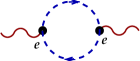
Figure 2: One loop contribution to the vacuum polarization from the 3-point interaction.

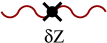
Figure 3: Photon field strength renormalization counterterm.

We represent the de Sitter background geometry in open conformal coordinates, which is conducive to regarding it as a limiting form of primordial inflation. The invariant element is

$$ds^{2}=a^{2}\left[-d\eta^{2}+d\vec{x}\cdot d\vec{x}\right]\;,$$ (2)

where $a(\eta)=-\frac{1}{H\eta}=e^{Ht}$ is the scale factor and $H$ is the Hubble parameter. Gravity is treated as a non-dynamical background, with the vector potential $A_{\mu}(x)$ and the complex scalar $\phi(x)$ being the dynamical variables. The Lagrangian describing massless SQED is

$$\mathcal{L}_{m=0}=-\frac{1}{4}F_{\mu\nu}F_{\rho\sigma}g^{\mu\rho}g^{\nu\sigma}\sqrt{-g}-(\partial_{\mu}-ieA_{\mu})\phi^{*}(\partial_{\nu}+ieA_{\nu})\phi g^{\mu\nu}\sqrt{-g}\;,$$ (3)

where $F_{\mu\nu}\equiv\partial_{\mu}A_{\nu}-\partial_{\nu}A_{\mu}$ is the field strength. The Lagrangian for massive SQED is

$$\mathcal{L}_{m\neq 0}=\mathcal{L}_{m=0}-M^{2}\phi^{*}\phi\sqrt{-g}\;,$$ (4)

where we are particularly interested in the case $M\ll H$.

In representing functions which depend upon two points, $x^{\mu}$ and ${x^{\prime}}^{\mu}$, we will make extensive use of the de Sitter length function

$$y(x;x^{\prime})\equiv a(\eta)a(\eta^{\prime})H^{2}\left[||\vec{x}-\vec{x}^{\prime}||^{2}-(|\eta-\eta^{\prime}|-i\delta)^{2}\right]\;.$$ (5)

We also have need of two de Sitter breaking combinations of the scale factor $a$ at $x^{\mu}$ and $a^{\prime}$ at ${x^{\prime}}^{\mu}$

$$u\equiv\ln(aa^{\prime})\;,\quad{\rm and}\quad v\equiv\ln\Bigl{(}\frac{a}{a^{\prime}}\Bigr{)}\;.$$ (6)

Derivatives of $y$ and $u$ furnish a convenient basis for representing bi-vector functions of $x^{\mu}$ and ${x^{\prime}}^{\mu}$ such as the vacuum polarization

$$\partial_{\mu}y\quad,\quad\partial^{\prime}_{\nu}y\quad,\quad\partial_{\mu}\partial^{\prime}_{\nu}y\quad,\quad\partial_{\mu}u\quad,\quad\partial^{\prime}_{\nu}u\;.$$ (7)

We do not need derivatives of $v$ because they are related to those of $u$

$$\partial_{\mu}v=\partial_{\mu}u\qquad,\qquad\partial^{\prime}_{\nu}v=-\partial^{\prime}_{\nu}u\;.$$ (8)

It turns out that either taking covariant derivatives of any of the five basis tensors (7), or contracting any two of them into one another, produces metrics and more basis tensors [13, 14].

Section 2 develops a representation, based on two covariant derivatives, for the vacuum polarization from a massless, minimally coupled scalar [1]. In this case there is de Sitter breaking, which requires two structure functions. When there is no de Sitter breaking the vacuum polarization can be expressed in terms of just a single structure function using a representation which involves four covariant derivatives. Section 3 derives this representation for the case of a massive scalar [2]. In section 4 we use the result of section 3 to study the effective field equations. An especially counter-intuitive and confusing feature of the de Sitter invariant representation is that local corrections to the effective field equations manifest as surface terms from the initial time. Section 5 comprises our discussion.

2 A Massless, Minimally Coupled Scalar

The purpose of this section is to express the one loop vacuum polarization from a massless, minimally coupled scalar using a neutral representation that would be manifestly de Sitter invariant if the physics was. In the first sub-section we review the primitive expression for the three diagrams of Figs. 1-3. The next sub-section derives the most general transverse form the vacuum polarization can take consistent with the symmetries of cosmology. In the final sub-section we give a simple solution for the structure functions which reproduces the primitive result.

2.1 The Primitive Result

If we call the scalar propagator $i\Delta(x;x^{\prime})$ then the three diagrams in Figs. 1-3 make the following contribution to the vacuum polarization

$$i\Bigl{[}\mbox{}^{\mu}\Pi^{\nu}\Bigr{]}(x;x^{\prime})=-2ie^{2}\sqrt{-g}\,g^{\mu\nu}i\Delta(x;x)\delta^{D}(x\!-\!x^{\prime})$$ (9)

$$+2e^{2}\sqrt{-g}\,g^{\mu\rho}\sqrt{-g^{\prime}}\,g^{\prime\nu\sigma}\Bigl{[}\partial_{\rho}i\Delta(x;x^{\prime})\partial^{\prime}_{\sigma}i\Delta(x;x^{\prime})\!-\!i\Delta(x;x^{\prime})\partial_{\rho}\partial^{\prime}_{\sigma}i\Delta(x;x^{\prime})\Bigr{]}$$

$$\hskip 99.58464pt+i\delta Z\partial_{\rho}\Bigl{[}\sqrt{-g}\Bigl{(}g^{\mu\nu}g^{\rho\sigma}\!-\!g^{\mu\sigma}g^{\nu\rho}\Bigr{)}\partial_{\sigma}\delta^{D}(x-x^{\prime})\Bigr{]}\;.\qquad$$

Equation (9) is valid for any scalar. For the special case of the massless, minimally coupled scalar the propagator obeys

$$\kern 1.0pt\vbox{\hrule height=1.2pt\hbox{\vrule width=1.2pt\hskip 3.0pt\vbox{\vskip 6.0pt}\hskip 3.0pt\vrule width=0.6pt}\hrule height=0.6pt}\kern 1.0pti\Delta_{A}(x;x^{\prime})=\frac{i\delta^{D}(x-x^{\prime})}{\sqrt{-g}}\;,$$ (10)

where $\kern 1.0pt\vbox{\hrule height=1.2pt\hbox{\vrule width=1.2pt\hskip 3.0pt\vbox{\vskip 6.0pt}\hskip 3.0pt\vrule width=0.6pt}\hrule height=0.6pt}\kern 1.0pt\equiv(-g)^{-\frac{1}{2}}\partial_{\mu}(\sqrt{-g}\,g^{\mu\nu}\partial_{\nu})$ is the covariant scalar d’Alembertian. It has long been known that equation (10) has no de Sitter invariant solution [12], so the scalar propagator must break some of the de Sitter symmetries. When using de Sitter as a paradigm for primordial inflation one obviously wishes to preserve the symmetries of cosmology: homogeneity, isotropy and spatial flatness. In that case the unique solution takes the form [15]

$$i\Delta_{A}(x;x^{\prime})=A\Bigl{(}y(x;x^{\prime})\Bigr{)}+k\ln(aa^{\prime})=A(y)+ku\;,$$ (11)

where the constant $k$ is

$$k=\frac{H^{D-2}}{(4\pi)^{\frac{D}{2}}}\frac{\Gamma(D\!-\!1)}{\Gamma(\frac{D}{2})}\;.$$ (12)

The de Sitter invariant part of the scalar propagator is

$$A(y)=\frac{H^{D-2}}{(4\pi)^{\frac{D}{2}}}\Biggl{\{}\frac{\Gamma(\frac{D}{2})}{\frac{D}{2}\!-\!1}\Bigl{(}\frac{4}{y}\Bigr{)}^{\frac{D}{2}-1}+\frac{\Gamma(\frac{D}{2}\!+\!1)}{\frac{D}{2}\!-\!2}\Bigl{(}\frac{4}{y}\Bigr{)}^{\frac{D}{2}-2}$$ (13)

$$\hskip 14.22636pt-\displaystyle\sum\limits_{n=1}^{\infty}\Biggl{[}\frac{\Gamma(n\!+\!\frac{D}{2}\!+\!1)}{(n\!-\!\frac{D}{2}\!+\!2)(n\!+\!1)!}\Bigl{(}\frac{y}{4}\Bigr{)}^{n-\frac{D}{2}+2}-\frac{\Gamma(n\!+\!D\!-\!1)}{n\Gamma(n\!+\!\frac{D}{2})}\Bigl{(}\frac{y}{4}\Bigr{)}^{n}\Biggr{]}\Biggr{\}}+A_{1},\qquad$$

where $A_{1}$ is a D-dependent constant which diverges for $D=4$

$$A_{1}=\frac{H^{D-2}}{(4\pi)^{D/2}}\frac{\Gamma(D\!-\!1)}{\Gamma(\frac{D}{2})}\Biggl{\{}-\psi\Bigl{(}1\!-\!\frac{D}{2}\Bigr{)}\!+\!\psi\Bigl{(}\frac{D\!-\!1}{2}\Bigr{)}\!+\!\psi(D\!-\!1)\!+\!\psi(1)\Biggr{\}}\;.$$ (14)

As a consequence of the propagator equation (10) the function $A(y)$ obeys

$$(4y\!-\!y^{2})A^{\prime\prime}(y)+D(2\!-\!y)A^{\prime}(y)=(D\!-\!1)k\;.$$ (15)

Derivatives of the propagator can be expressed using the tensor basis (7)

$$\partial_{\mu}i\Delta_{A}(x;x^{\prime}) = A^{\prime}(y)\times\partial_{\mu}y+k\times\partial_{\mu}u\;,$$ (16)

$$\partial^{\prime}_{\nu}i\Delta_{A}(x;x^{\prime}) = A^{\prime}(y)\times\partial^{\prime}_{\nu}y+k\times\partial^{\prime}_{\nu}u\;,$$ (17)

$$\partial_{\mu}\partial^{\prime}_{\nu}i\Delta_{A}(x;x^{\prime}) = A^{\prime}(y)\times\partial_{\mu}\partial^{\prime}_{\nu}y+A^{\prime\prime}(y)\times\partial_{\mu}y\,\partial^{\prime}_{\nu}y$$ (18)

$$\hskip 113.81102pt+\frac{i\delta^{D}(x\!-\!x^{\prime})}{H^{2}\sqrt{-g}}\times\partial_{\mu}u\,\partial^{\prime}_{\nu}u\;.\qquad$$

By applying these identities we can write (9) as

$$i\Bigl{[}\mbox{}^{\mu}\Pi^{\nu}\Bigr{]}(x;x^{\prime})=-2ie^{2}\sqrt{-g}\,g^{\mu\rho}g^{\nu\sigma}\Bigl{[}g_{\rho\sigma}\!+\!H^{-2}\partial_{\rho}u\partial_{\sigma}u\Bigr{]}(A_{1}\!+\!ku)\delta^{D}(x\!-\!x^{\prime})$$ (19)

$$+2e^{2}\sqrt{-g}\,g^{\mu\rho}\sqrt{-g^{\prime}}\,g^{\prime\nu\sigma}\Biggl{\{}\partial_{\rho}y\partial^{\prime}_{\sigma}y\!\times\!\Bigl{(}A^{\prime 2}\!-\!AA^{\prime\prime}\!-\!kuA^{\prime\prime}\Bigr{)}$$

$$-\partial_{\rho}\partial^{\prime}_{\sigma}y\!\times\!\Bigl{(}AA^{\prime}\!+\!kuA^{\prime}\Bigr{)}\!+\!\partial_{\rho}u\partial^{\prime}_{\sigma}y\times kA^{\prime}\!+\!\partial_{\rho}y\partial^{\prime}_{\sigma}u\!\times\!kA^{\prime}\!+\!\partial_{\rho}u\partial^{\prime}_{\sigma}u\!\times\!k^{2}\Biggr{\}}$$

$$\hskip 99.58464pt+i\delta Z\partial_{\rho}\Bigl{[}\sqrt{-g}\Bigl{(}g^{\mu\nu}g^{\rho\sigma}\!-\!g^{\mu\sigma}g^{\nu\rho}\Bigr{)}\partial_{\sigma}\delta^{D}(x-x^{\prime})\Bigr{]}\;.\qquad$$

The presence of de Sitter breaking in (19) is evident from the dependence upon $u$ and its derivatives.

2.2 General Representations

We wish to express (19) using a manifestly transverse representation analogous to the form (1) used for flat space. An important property of this representation is that it should be “neutral”. That is, it should be in terms of covariant derivatives so that the structure functions will be de Sitter invariant if the physical result happens to possess that symmetry. We are therefore led to the ansatz

$$i\Bigl{[}\mbox{}^{\mu}\Pi^{\nu}\Bigr{]}(x;x^{\prime})=\sqrt{-g(x)}\,\sqrt{-g(x^{\prime})}\,D_{\rho}D^{\prime}_{\sigma}\Bigl{[}\mbox{}^{\mu\rho}T^{\nu\sigma}\Bigr{]}(x;x^{\prime})\;,$$ (20)

where the bi-tensor $[\mbox{}^{\mu\rho}T^{\nu\sigma}](x;x^{\prime})$ must be antisymmetric under $\mu\leftrightarrow\rho$ and $\nu\leftrightarrow\sigma$. It must also obey the “reflection identity”

$$\Bigl{[}\mbox{}^{\mu\rho}T^{\nu\sigma}\Bigr{]}(x;x^{\prime})=\Bigl{[}\mbox{}^{\nu\sigma}T^{\mu\rho}\Bigr{]}(x^{\prime};x)\;.$$ (21)

The most general tensor satisfying these criteria, consistent with homogeneity and isotropy, is

$$\Bigl{[}\mbox{}_{\mu\rho}T_{\nu\sigma}\Bigr{]}=\partial_{\mu}\partial^{\prime}_{[\nu}y\,\partial^{\prime}_{\sigma]}\partial_{\rho}y\!\times\!f_{1}+\partial_{[\mu}y\,\partial_{\rho]}\partial^{\prime}_{[\nu}y\,\partial^{\prime}_{\sigma]}y\!\times\!f_{2}+\partial_{[\mu}y\,\partial_{\rho]}\partial^{\prime}_{[\nu}y\,\partial^{\prime}_{\sigma]}u\!\times\!f_{3}$$ (22)

$$+\partial_{[\mu}u\,\partial_{\rho]}\partial^{\prime}_{[\nu}y\partial^{\prime}_{\sigma]}y\!\times\!\tilde{f}_{3}+\partial_{[\mu}u\,\partial_{\rho]}\partial^{\prime}_{[\nu}y\,\partial^{\prime}_{\sigma]}u\!\times\!f_{4}+\partial_{[\mu}y\,\partial_{\rho]}u\,\partial^{\prime}_{[\nu}y\partial^{\prime}_{\sigma]}u\!\times\!f_{5}\;.\qquad$$

Here the scalar structure functions $f_{i}(y,u,v)$ depend on $y$, $u$ and $v$, and we define $\tilde{f}_{3}(y,u,v)\equiv f_{3}(y,u,-v)$. Of course manifest de Sitter invariance precludes $f_{3},f_{4}$ and $f_{5}$, and we will in the end employ only $f_{1}$ and $f_{2}$.

There is obviously some redundancy in the five structure functions of (22) because acting the derivatives in (20) results in only four algebraically independent tensors,

$$D^{\rho}{D^{\prime}}^{\sigma}\Bigl{[}\mbox{}_{\mu\rho}T_{\nu\sigma}\Bigr{]}(x;x^{\prime})=\partial_{\mu}\partial^{\prime}_{\nu}y\!\times\!F_{1}\!+\!\partial_{\mu}y\,\partial^{\prime}_{\nu}y\!\times\!F_{2}$$ (23)

$$\hskip 113.81102pt+\partial_{\mu}u\,\partial^{\prime}_{\nu}y\!\times\!F_{3}\!+\!\partial_{\mu}y\,\partial^{\prime}_{\nu}u\!\times\!\widetilde{F}_{3}\!+\!\partial_{\mu}u\,\partial^{\prime}_{\nu}u\!\times\!F_{4}\;.\qquad$$

Conservation implies two differential relations [14],

$$\Bigl{[}-(2\!-y)\partial_{y}\!+\!D\!+\!\partial_{u}\!+\!\partial_{v}\!+\!2e^{-v}\partial_{y}\Bigr{]}F_{3}=\Bigl{[}(2\!-\!y)\partial_{y}\!-\!D\!-\!\partial_{u}\!-\!\partial_{v}\Bigr{]}F_{1}$$ (24)

$$\hskip 51.21504pt+\Bigl{[}(4y\!-\!y^{2})\partial_{y}\!+\!(D\!+\!1)(2\!-\!y)\!+\!(2\!-\!y\!-\!2e^{-v})(\partial_{u}\!+\!\partial_{v})\Bigr{]}F_{2}\;,\qquad$$

$$\Bigl{[}-(2\!-\!y)\partial_{y}\!+\!(D\!-\!1)\!+\!\partial_{u}\!+\!\partial_{v}\!+\!2e^{-v}\partial_{y}\Bigr{]}F_{4}=-2e^{-v}(\partial_{u}\!+\!\partial_{v})F_{1}\!-\!2e^{-v}F_{3}$$ (25)

$$\hskip 76.82234pt+\Bigl{[}(4y\!-\!y^{2})\partial_{y}\!+\!D(2\!-\!y)\!+\!(2\!-\!y\!-\!2e^{-v})(\partial_{u}\!+\!\partial_{v})\Bigr{]}\widetilde{F}_{3}\;.\qquad$$

This suggests that one should be able to write the scalar coefficient functions $F_{i}(y,u,v)$ of expression (23) in terms of just two master structure functions, which we might call $\Phi(y,u,v)$ and $\Psi(y,u,v)$. After long reflection, one sees that the following substitutions for the $F_{i}(y,u,v)$ reduce the conservation relations (24-25) to tautologies,

$$F_{1}\!\!\! = \!\!\!\Bigl{[}-(4y\!-\!y^{2})\partial_{y}\!-\!(D\!-\!1)(2\!-\!y)\!-\!2(2\!-\!y)\partial_{u}\!+\!4\cosh(v)\partial_{u}\!-\!4\sinh(v)\partial_{v}\Bigr{]}\Phi$$ (26)

$$\hskip 184.9429pt+\Bigl{[}4\cosh(v)\!-\!(2\!-\!y)\Bigr{]}\Psi\!-\!\Xi\;,\qquad$$

$$F_{2}\!\!\! = \!\!\!\Bigl{[}(2\!-\!y)\partial_{y}\!-\!D\!+\!1\!-\!2\partial_{u}\Big{]}\Phi\!-\!\Psi\;,\qquad$$ (27)

$$F_{3}\!\!\! = \!\!\!-2e^{v}(\partial_{u}\!-\!\partial_{v})\Phi\!-\!2e^{v}\Psi\!+\!\Xi\;,$$ (28)

$$\widetilde{F}_{3}\!\!\! = \!\!\!-2e^{-v}(\partial_{u}\!+\!\partial_{v})\Phi\!-\!2e^{-v}\Psi\!+\!\Xi\;,$$ (29)

$$F_{4}\!\!\! = \!\!\!-4\Psi\!+\!(2\!-\!y)\Xi\;.$$ (30)

Here the auxiliary function $\Xi(y,u,v)$ is,

$$\Xi(y,u,v)\equiv\int\!\!dy\,(\partial_{u}^{2}\!-\!\partial_{v}^{2})\Phi(y,u,v)\!+\!(2\!-\!y)\Psi(y,u,v)\!-\!(D\!-\!2)\!\!\int\!\!dy\,\Psi(y,u,v)\;.$$ (31)

Tensor	Coefficient
$\partial^{\mu}\partial^{\prime\nu}y$	$-(D-1)^{2}(2-y)f_{1}+\left[(D-1)(2-y)^{2}-D(4y-y^{2})\right]\partial_{y}f_{1}$
	$+(2-y)(4y-y^{2})\partial_{y}^{2}f_{1}-2(D-1)(2-y)\partial_{u}f_{1}$
	$+2\left(\frac{a}{a^{\prime}}+\frac{a^{\prime}}{a}\right)\left[(D-1)\partial_{u}f_{1}-(2-y)\partial_{u}\partial_{y}f_{1}\right]$
	$-2\left(\frac{a}{a^{\prime}}-\frac{a^{\prime}}{a}\right)\left[(D-1)\partial_{v}f_{1}-(2-y)\partial_{v}\partial_{y}f_{1}\right]$
	$+2(2-y)^{2}\partial_{u}\partial_{y}f_{1}+\left[2\left(\frac{a}{a^{\prime}}+\frac{a^{\prime}}{a}\right)-(2-y)\right](\partial_{u}^{2}-\partial_{v}^{2})f_{1}$
$\partial^{\mu}y\partial^{\prime\nu}y$	$-(D-1)^{2}f_{1}+(2D-1)(2-y)\partial_{y}f_{1}-(2-y)^{2}\partial^{2}_{y}f_{1}$
	$-2(D-1)\partial_{u}f_{1}+2(2-y)\partial_{u}\partial_{y}f_{1}-(\partial_{u}^{2}-\partial_{v}^{2})f_{1}$
$\partial^{\mu}y\partial^{\prime\nu}u$	$2\frac{a^{\prime}}{a}\left[-(D-1)(\partial_{u}+\partial_{v})f_{1}+(2-y)(\partial_{u}+\partial_{v})\partial_{y}f_{1}\right.$
	$\left.-(\partial_{u}^{2}-\partial_{v}^{2})f_{1}\right]$
$\partial^{\mu}u\partial^{\prime\nu}y$	$2\frac{a}{a^{\prime}}\left[-(D-1)(\partial_{u}-\partial_{v})f_{1}+(2-y)(\partial_{u}-\partial_{v})\partial_{y}f_{1}\right.$
	$\left.-(\partial_{u}^{2}-\partial_{v}^{2})f_{1}\right]$
$\partial^{\mu}u\partial^{\prime\nu}u$	$-4(\partial_{u}^{2}-\partial_{v}^{2})f_{1}$

Table 1: Result for expanding $D_{\rho}D^{\prime}_{\sigma}\left[(\partial^{\mu}\partial^{\prime[\nu}y)(\partial^{\prime\sigma]}\partial^{\rho}y)f_{1}(y,u,v)\right]$; all coefficients are multiplied by a factor of $\frac{1}{2}H^{4}$.

Given the coefficient functions $F_{i}(y,u,v)$, one can derive a first order differential equation in one variable for the master structure function $\Phi(y,u,v)$ by taking a superposition of relations (26-30),

$$-4(D\!-\!1)\Phi\!-\!8\partial_{u}\Phi=(2\!-\!y)F_{1}\!+\!(4y\!-\!y^{2})F_{2}\!+\!(2\!-\!y)(F_{3}\!+\!\widetilde{F}_{3})\!-\!F_{4}\;.\qquad$$ (32)

The difference of (28) and (29) gives an algebraic relation for $\Psi(y,u,v)$ once $\Phi(y,u,v)$ is known,

$$-4\sinh(v)\partial_{u}\Phi\!+\!4\cosh(v)\partial_{v}\Phi\!-\!4\sinh(v)\Psi=F_{3}\!-\!\widetilde{F}_{3}\;.\qquad$$ (33)

Note that de Sitter invariance implies $\Phi=\Phi(y)$ and $\Psi=0$.

Tensor	Coefficient
$\partial^{\mu}\partial^{\prime\nu}y$	$\left[-D(D-1)(2-y)^{2}+D(4y-y^{2})\right]f_{2}-(4y-y^{2})^{2}\partial_{y}^{2}f_{2}$
	$-(2D+1)(2-y)(4y-y^{2})\partial_{y}f_{2}-2D(2-y)^{2}\partial_{u}f_{2}$
	$+2\left(\frac{a}{a^{\prime}}+\frac{a^{\prime}}{a}\right)\left[D(2-y)\partial_{u}f_{2}+(4y-y^{2})\partial_{u}\partial_{y}f_{2}\right]$
	$-2\left(\frac{a}{a^{\prime}}-\frac{a^{\prime}}{a}\right)\left[D(2-y)\partial_{v}f_{2}+(4y-y^{2})\partial_{v}\partial_{y}f_{2}\right]$
	$-2(2-y)(4y-y^{2})\partial_{u}\partial_{y}f_{2}-(8-4y+y^{2})(\partial_{u}^{2}-\partial^{2}_{v})f_{2}$
	$+2(2-y)\left(\frac{a}{a^{\prime}}+\frac{a^{\prime}}{a}\right)(\partial^{2}_{u}-\partial_{v}^{2})f_{2}$
$\partial^{\mu}y\partial^{\prime\nu}y$	$-D^{2}(2-y)f_{2}+\left[-(D-1)(4y-y^{2})+(D+2)(2-y)^{2}\right]\partial_{y}f_{2}$
	$+(2-y)(4y-y^{2})\partial_{y}^{2}f_{2}-2D(2-y)\partial_{u}f_{2}$
	$-2(4y-y^{2})\partial_{u}\partial_{y}f_{2}-(2-y)(\partial_{u}^{2}-\partial_{v}^{2})f_{2}$
$\partial^{\mu}y\partial^{\prime\nu}u$	$-2\frac{a^{\prime}}{a}\left[D(2-y)(\partial_{u}+\partial_{v})f_{2}+(4y-y^{2})(\partial_{u}+\partial_{v})\partial_{y}f_{2}\right]$
	$+\left[4-2(2-y)\frac{a^{\prime}}{a}\right](\partial^{2}_{u}-\partial_{v}^{2})f_{2}$
$\partial^{\mu}u\partial^{\prime\nu}y$	$-2\frac{a}{a^{\prime}}\left[D(2-y)(\partial_{u}-\partial_{v})f_{2}+(4y-y^{2})(\partial_{u}-\partial_{v})\partial_{y}f_{2}\right]$
	$+\left[4-2(2-y)\frac{a}{a^{\prime}}\right](\partial^{2}_{u}-\partial_{v}^{2})f_{2}$
$\partial^{\mu}u\partial^{\prime\nu}u$	$0$

Table 2: Result for expanding $D_{\rho}D^{\prime}_{\sigma}\left[(\partial^{[\mu}y)(\partial^{\rho]}\partial^{\prime[\nu}y)(\partial^{\prime\sigma]}y)f_{2}(y,u,v)\right]$; all coefficients are multiplied by a factor of $\frac{1}{4}H^{4}$.

It remains to relate the master structure functions $\Phi(y,u,v)$ and $\Psi(y,u,v)$ to the structure functions $f_{i}(y,u,v)$ of our representation (20-22). Table 1 gives the coefficient functions $F_{i}(y,u,v)$ for the structure function $f_{1}(y,u,v)$. Applying relations (32-33) implies that the associated master structures are,

$$\Phi_{1} = \frac{H^{4}}{2}\Bigl{\{}(D\!-\!1)f_{1}\!-\!(2\!-\!y)\partial_{y}f_{1}\Bigr{\}}\;,$$ (34)

$$\Psi_{1} = \frac{H^{4}}{2}\Bigl{\{}(\partial_{u}^{2}\!-\!\partial_{v}^{2})f_{1}\Bigr{\}}\;.$$ (35)

Table 2 gives the coefficient functions $F_{i}(y,u,v)$ for $f_{2}(y,u,v)$, from which we infer,

$$\Phi_{2} = \frac{H^{4}}{4}\Bigl{\{}D(2\!-\!y)f_{2}\!+\!(4y\!-\!y^{2})\partial_{y}f_{2}\Bigr{\}}\;,$$ (36)

$$\Psi_{2} = \frac{H^{4}}{4}\Bigl{\{}(2\!-\!y)(\partial_{u}^{2}\!-\!\partial_{v}^{2})f_{2}\Bigr{\}}\;.$$ (37)

The master structure functions for $f_{3}(y,u,v)$ and $\widetilde{f}_{3}(y,u,v)=f_{3}(y,u,-v)$ are,

$$\Phi_{3} = \frac{H^{4}}{4}\Bigl{\{}-(D\!-\!1)(f_{3}\!+\!\widetilde{f}_{3})\!+\!(2\!-\!y)\partial_{y}(f_{3}\!+\!\widetilde{f}_{3})\!-\!2\partial_{y}(e^{v}f_{3}\!+\!e^{-v}\widetilde{f}_{3})\Bigr{\}}\;,\qquad$$ (38)

$$\Psi_{3} = \!\frac{H^{4}}{4}\Bigl{\{}2\partial_{y}\Big{[}\partial_{u}(e^{v}f_{3}\!+\!e^{-v}\widetilde{f}_{3})\!-\!\partial_{v}(e^{v}f_{3}\!-\!e^{-v}\widetilde{f}_{3})\Big{]}\!-\!(\partial_{u}^{2}\!-\!\partial_{v}^{2})(f_{3}\!+\!\widetilde{f}_{3})\Bigr{\}}.\qquad$$ (39)

The analogous result for $f_{4}(y,u,v)$ is,

$$\Phi_{4} = \frac{H^{4}}{4}\Bigl{\{}\partial_{y}f_{4}\Bigr{\}}\;,$$ (40)

$$\Psi_{4} = \frac{H^{4}}{4}\Bigl{\{}-(D\!-\!1)\partial_{y}f_{4}\!+\!(2\!-\!y)\partial_{y}^{2}f_{4}\!-\!2\partial_{y}\partial_{u}f_{4}\Bigr{\}}\;.\qquad$$ (41)

And $f_{5}(y,u,v)$ gives,

$$\Phi_{5}\!\!\!\!\! = \!\!\!\!\!\frac{H^{4}}{4}\Bigl{\{}-Df_{5}\!+\!2(2\!-\!y)\partial_{y}f_{5}\!-\!4\cosh(v)\partial_{y}f_{5}\Bigr{\}}\;,$$ (42)

$$\Psi_{5}\!\!\!\!\! = \!\!\!\!\!\frac{H^{4}}{4}\Bigl{\{}\!(D\!-\!1)f_{5}\!-\!(D\!+\!1)(2\!-\!y)]\partial_{y}f_{5}\!-\!(4y\!-\!y^{2})\partial_{y}^{2}f_{5}\!+\!2\partial_{u}f_{5}$$ (43)

$$+[-\!2(2\!-\!y)\!+\!4\cosh(v)]\partial_{u}\partial_{y}f_{5}\!-\!4\partial_{v}\partial_{y}[\sinh(v)f_{5}]-(\partial_{u}^{2}\!-\!\partial_{v}^{2})f_{5}\Bigr{\}}\;.\qquad$$

From these expressions one sees that the vacuum polarization can be described in terms of any two of the structure functions $f_{i}(y,u,v)$. When the result is de Sitter invariant then it requires only a single structure function, which can be either $f_{1}(y)$ or $f_{2}(y)$.

2.3 Representation for this System

It remains to work out the structure functions for the primitive result (19). Substituting the coefficient functions $F_{i}(y,u,v)$ from expression (19) into relation (32), and making judicious use of the $A$ propagator equation (15), gives the first master structure function,

$$\Phi = -\frac{e^{2}}{2(D\!-\!1)}\biggl{[}(D\!-\!1)[(2\!-\!y)A^{\prime}\!-\!k]A\!+\!(4y\!-\!y^{2}){A^{\prime}}^{2}\biggr{]}$$ (44)

$$-\frac{ke^{2}}{2}[(2\!-\!y)A^{\prime}\!-\!k]u\;,$$

where we dropped local terms $\propto\delta^{D}(x-x^{\prime})$ and also the prefactor $\sqrt{-g}\sqrt{-g^{\prime}}={\rm e}^{Du}$ in (19), as it contributes to the integral measure to make it covariant. Doing the same thing for relation (33) implies that the second master structure function is,

$$\Psi=\frac{ke^{2}}{2}[(2\!-\!y)A^{\prime}\!-\!k]\;.$$ (45)

At this point we must make a choice between the ten possible pairs of structure functions $f_{i}(y,u,v)$ that could be used to represent the result. We chose $f_{1}$ and $f_{2}$, the two structure functions that would be de Sitter invariant if the system was. In view of relations (35), (37) and (45), the requirement that $\Psi_{1}+\Psi_{2}=\Psi$ implies the form,

$$f_{1}(y,u,v) = -\frac{k^{2}e^{2}}{4H^{4}}\,(u^{2}\!-\!v^{2})+f_{1a}(y,u\!+\!v)+f_{1b}(y,u\!-\!v)\;,$$ (46)

$$f_{2}(y,u,v) = \frac{ke^{2}}{2H^{4}}\,A^{\prime}(y)(u^{2}\!-\!v^{2})+f_{2a}(y,u\!+\!v)+f_{2b}(y,u\!-\!v)\;.\quad$$ (47)

Then requiring $\Phi_{1}+\Phi_{2}=\Phi$ and relations (34), (36), and (44) implies,

$$f_{1}(y,u,v) = -\frac{k^{2}e^{2}}{4H^{4}}\,(u^{2}-v^{2})+\alpha_{1}(y)u+\alpha_{2}(y)\;,$$ (48)

$$f_{2}(y,u,v) = \frac{ke^{2}}{2H^{4}}\,A^{\prime}(y)(u^{2}-v^{2})+\beta_{1}(y)u+\beta_{2}(y)\;,$$ (49)

where the functions $\alpha_{i}(y)$ and $\beta_{i}(y)$ satisfy,

$$-\frac{2ke^{2}}{H^{4}}[(2\!-\!y)A^{\prime}\!-\!k]$$

$$\hskip 85.35826pt=\,2(D\!-\!1)\alpha_{1}\!-\!2(2\!-\!y)\alpha_{1}^{\prime}\!+\!D(2\!-\!y)\beta_{1}\!+\!(4y-y^{2})\beta_{1}^{\prime}\;,\qquad$$ (50)

$$-\frac{2e^{2}}{(D\!-\!1)H^{4}}\Bigl{\{}(D\!-\!1)[(2\!-\!y)A^{\prime}\!-\!k]A\!+\!(4y\!-\!y^{2}){A^{\prime}}^{2}+\,k^{2}\Bigr{\}}$$

$$\hskip 85.35826pt=\,2(D\!-\!1)\alpha_{2}\!-\!2(2\!-\!y)\alpha_{2}^{\prime}\!+\!D(2\!-\!y)\beta_{2}\!+\!(4y-y^{2})\beta_{2}^{\prime}\;.\qquad$$ (51)

Because we have only two equations (50-51) in terms of four functions $\alpha_{i}(y)$ and $\beta_{i}(y)$, there are many solutions. Perhaps the nicest — and one of great significance for the next section — results from the ansatz,

$$\alpha_{i}(y)=\gamma_{i}^{\prime}(y)\qquad,\qquad\beta_{i}(y)=-\gamma_{i}^{\prime\prime}(y)\;.$$ (52)

This ansatz effects the following simplification of the right hand sides of (50-51),

$$2(D\!-\!1)\alpha_{i}(y)\!-\!2(2\!-\!y)\alpha_{i}^{\prime}(y)\!+\!D(2\!-\!y)\beta_{i}(y)\!+\!(4y-y^{2})\beta_{i}^{\prime}(y)$$ (54)

$$\hskip 68.28644pt=-\frac{\partial}{\partial y}\Bigl{[}(4y\!-\!y^{2})\gamma_{i}^{\prime\prime}(y)\!+\!D(2\!-\!y)\gamma^{\prime}_{i}(y)\!-\!(D\!-\!2)\gamma_{i}(y)\Bigr{]}\;,\qquad$$

$$\hskip 68.28644pt=-\frac{d}{dy}\Bigl{[}\frac{\kern 1.0pt\vbox{\hrule height=1.2pt\hbox{\vrule width=1.2pt\hskip 3.0pt\vbox{\vskip 6.0pt}\hskip 3.0pt\vrule width=0.6pt}\hrule height=0.6pt}\kern 1.0pt}{H^{2}}\!-\!(D\!-\!2)\Bigr{]}\gamma_{i}(y)\equiv-\frac{d}{dy}\frac{D_{B}}{H^{2}}\gamma_{i}(y)\;.$$

One can see from relation (54) that it would be highly desirable to express the left hand sides of (50-51) as $\partial/\partial y$ of something. The desired function involves the propagator of a scalar with mass $M^{2}=(D-2)H^{2}$, which obeys the equation,

$$D_{B}i\Delta_{B}(x;x^{\prime})=\frac{i\delta^{D}(x\!-\!x^{\prime})}{\sqrt{-g}}\;.$$ (55)

Unlike the massless scalar, the propagator of this massive scalar can be expressed in terms of a de Sitter invariant function of $y$, $i\Delta_{B}(x;x^{\prime})=B(y)$. The series expansion of this function is,

$$B(y)=\frac{H^{D-2}}{(4\pi)^{\frac{D}{2}}}\Biggl{\{}\Gamma\Bigl{(}\frac{D}{2}\!-\!1\Bigr{)}\Bigl{(}\frac{4}{y}\Bigr{)}^{\frac{D}{2}-1}+\sum_{n=0}^{\infty}\Biggr{[}\frac{\Gamma(n\!+\!\frac{D}{2})}{\Gamma(n\!+\!2)}\Bigl{(}\frac{y}{4}\Bigr{)}^{n-\frac{D}{2}+2}$$ (56)

$$\hskip 190.63338pt-\frac{\Gamma(n\!+\!D\!-\!2)}{\Gamma(n\!+\!\frac{D}{2})}\Bigl{(}\frac{y}{4}\Bigr{)}^{n}\Biggr{]}\Biggr{\}}\;.\qquad$$

The series expansions (13) and (56) imply two relations between $A(y)$ and $B(y)$ of great utility,

$$(2\!-\!y)A^{\prime}(y)\!-\!k = 2B^{\prime}(y)\;,$$ (57)

$$(4y\!-\!y^{2})A^{\prime}(y)+k(2\!-\!y) = -2(D\!-\!2)B(y)\;.$$ (58)

Relation (57) implies that our ansatz (52) reduces equation (50) to the form,

$$D_{B}\gamma_{1}(y)=\frac{4ke^{2}}{H^{2}}\,B(y)\;.$$ (59)

The solution is,

$$\gamma_{1}(y)=\frac{4ke^{2}}{H^{2}}\,i\Delta_{BB}(x;x^{\prime})\;,$$ (60)

where the de Sitter invariant biscalar $i\Delta_{BB}(x;x^{\prime})$ was introduced in a previous study of the graviton propagator [16]. Using relation (58) similarly on (51) implies,

$$D_{B}\gamma_{2}(y)=\frac{4e^{2}}{(D\!-\!1)H^{2}}\int\!\!dy\Bigl{\{}(D\!-\!1)A(y)B^{\prime}(y)-(D\!-\!2)A^{\prime}(y)B(y)-kB^{\prime}(y)\Bigr{\}}\;.$$ (61)

In the next section we will derive a de Sitter invariant Green’s function which can be used to solve for $\gamma_{2}(y)$.

3 A Massive Scalar

The purpose of this section is to derive a de Sitter invariant representation for the one loop vacuum polarization from a charged scalar with a small mass. The first subsection is devoted to presenting the primitive result from the three diagrams in Figs 1-3, with special attention to the expansion of the massive scalar propagator for small mass. In the second subsection we re-express the primitive result . It is at this point that we derive the Green’s function for the differential operator $D_{B}$ defined in (54). The final subsection explains renormalization.

3.1 The Primitive Result

The propagator of a minimally coupled scalar of mass $M$ obeys the equation,

$$(\kern 1.0pt\vbox{\hrule height=1.2pt\hbox{\vrule width=1.2pt\hskip 3.0pt\vbox{\vskip 6.0pt}\hskip 3.0pt\vrule width=0.6pt}\hrule height=0.6pt}\kern 1.0pt\!-\!M^{2})i\Delta_{T}(x;x^{\prime})=\frac{i\delta^{D}(x\!-\!x^{\prime})}{\sqrt{-g}}\;.$$ (62)

For $M^{2}>0$ it has a de Sitter invariant solution $i\Delta_{T}(x;x^{\prime})=T(y)$,

$$T(y)=\frac{H^{D-2}}{(4\pi)^{\frac{D}{2}}}\frac{\Gamma(\frac{D-1}{2}\!+\!\nu)\Gamma(\frac{D-1}{2}\!-\!\nu)}{\Gamma(\frac{D}{2})}\,\mbox{}_{2}F_{1}\Bigl{(}\frac{D-1}{2}\!+\!\nu;\frac{D-1}{2}\!-\!\nu;\frac{D}{2};1\!-\!\frac{y}{4}\Bigr{)}\;,$$ (63)

where $\nu\equiv\sqrt{\left(\frac{D-1}{2}\right)^{2}-\frac{M^{2}}{H^{2}}}$ [17]. (The $B$-type propagator (55-56) represents the special case of $M^{2}=(D-2)H^{2}$.) It is useful to extract the most ultraviolet singular term from $T(y)$,

$$T(y)\equiv\frac{H^{D-2}}{4\pi^{\frac{D}{2}}}\Gamma\Bigl{(}\frac{D}{2}\!-\!1\Bigr{)}\left[\frac{1}{y^{\frac{D}{2}-1}}+\Delta T(y)\right]\equiv K\left[\frac{1}{y^{\frac{D}{2}-1}}+\Delta T(y)\right]\;.$$ (64)

Just as in flat space, nonzero mass greatly complicates the spacetime dependence of propagators. For example, the series expansion of $\Delta T(y)$ in powers of $y$ does not terminate in $D=4$ dimensions for most choices of $M^{2}>0$. One signal that there is no de Sitter invariant solution for the massless case is that $\Delta T(y)$ diverges as $M$ goes to zero. This can be quantified by giving the Laurent expansion for $\Delta T(y)$ in terms of the parameter $s\equiv(\frac{D-1}{2})-\nu$. In $D=4$ dimensions, we have [2],

$$\Delta T(y)=\frac{1}{2s}-\frac{1}{2}\ln\Bigl{(}\frac{y}{4}\Bigr{)}-1+s\!\times\!\delta T(y)+O(s^{2})\;,$$ (65)

where the function $\delta T(y)$ is,

$$\delta T(y)=\frac{1}{2}{\rm Li}_{2}\Bigl{(}\frac{y}{4}\Bigr{)}+\ln\Bigl{(}\frac{y}{4}\Bigr{)}\biggl{[}\frac{1}{2}\ln\Bigl{(}1-\frac{y}{4}\Bigr{)}+1-\frac{1}{4-y}\biggr{]}\,,$$ (66)

and where ${\rm Li}_{2}(z)=\sum_{n=1}^{\infty}z^{n}/n^{2}$ is the polylogarithm function. For small mass the $1/s$ contribution to the vacuum polarization is the dominant effect.

Substituting $i\Delta_{T}(x;x^{\prime})$ for the scalar propagator in expression (9) gives the result for the three diagrams of Figs 1-3. Derivatives of the propagator can be expressed using the tensor basis (7)

$$\partial_{\mu}i\Delta_{T}(x;x^{\prime}) = T^{\prime}(y)\times\partial_{\mu}y\;,$$ (67)

$$\partial^{\prime}_{\nu}i\Delta_{T}(x;x^{\prime}) = T^{\prime}(y)\times\partial^{\prime}_{\nu}y\;,$$ (68)

$$\partial_{\mu}\partial^{\prime}_{\nu}i\Delta_{T}(x;x^{\prime}) = T^{\prime}(y)\times\partial_{\mu}\partial^{\prime}_{\nu}y+T^{\prime\prime}(y)\times\partial_{\mu}y\,\partial^{\prime}_{\nu}y$$ (69)

$$\hskip 113.81102pt+\frac{i\delta^{D}(x\!-\!x^{\prime})}{H^{2}\sqrt{-g}}\times\partial_{\mu}u\,\partial^{\prime}_{\nu}u\;.\qquad$$

By applying these identities we can write (9) as

$$i\Bigl{[}\mbox{}^{\mu}\Pi^{\nu}\Bigr{]}(x;x^{\prime})=\sqrt{-g(x)}\,g^{\mu\rho}(x)\sqrt{-g(x^{\prime})}\,g^{\nu\sigma}(x^{\prime})\biggl{\{}\partial_{\rho}\partial^{\prime}_{\sigma}y\!\times\!(-2e^{2}TT^{\prime})$$ (70)

$$\hskip 14.22636pt+\partial_{\rho}y\partial^{\prime}_{\sigma}y\!\times\!2e^{2}\Bigl{(}{T^{\prime}}^{2}\!-\!TT^{\prime\prime}\Bigr{)}\!-\!2e^{2}T(0)\Bigl{[}g_{\rho\sigma}\!+\!H^{-2}\partial_{\rho}u\partial_{\sigma}u\Bigr{]}\frac{i\delta^{D}(x\!-\!x^{\prime})}{\sqrt{-g}}$$

$$\hskip 85.35826pt+\delta Z\biggl{[}g_{\rho\sigma}\Bigl{[}\kern 1.0pt\vbox{\hrule height=1.2pt\hbox{\vrule width=1.2pt\hskip 3.0pt\vbox{\vskip 6.0pt}\hskip 3.0pt\vrule width=0.6pt}\hrule height=0.6pt}\kern 1.0pt\!+\!(D\!-\!1)H^{2}\Bigr{]}\!-\!D_{\rho}D_{\sigma}\biggr{]}\frac{i\delta^{D}(x-x^{\prime})}{\sqrt{-g}}\biggr{\}}\;,\qquad$$

where

$$T(0)=\frac{H^{D-2}}{(4\pi)^{\frac{D}{2}}}\frac{\Gamma(\frac{D-1}{2}\!+\!\nu)\Gamma(\frac{D-1}{2}\!-\!\nu)}{\Gamma(\frac{1}{2}+\nu)\Gamma(\frac{1}{2}-\nu)}\,.$$

3.2 The $\gamma(y)$ Representation

Because the primitive result (70) is de Sitter invariant, it can be given a manifestly de Sitter invariant expression using the structure functions $f_{1}(y)$ and $f_{2}(y)$ of our general representation (20-22). A further simplification arises if we relate the structure functions as $f_{1}(y)=\gamma^{\prime}(y)$ and $f_{2}(y)=-\gamma^{\prime\prime}(y)$,

$$i\Bigl{[}\mbox{}^{\mu}\Pi^{\nu}\Bigr{]}(x;x^{\prime})=\sqrt{-g(x)}\,g^{\mu\rho}(x)\sqrt{-g(x^{\prime})}\,g^{\nu\sigma}(x^{\prime})\times D^{\alpha}{D^{\prime}}^{\beta}$$ (72)

$$\hskip 71.13188pt\times\Biggl{\{}\partial_{\rho}\partial^{\prime}_{[\sigma}y\,\partial^{\prime}_{\beta]}\partial_{\alpha}y\!\times\!\gamma^{\prime}(y)\!-\!\partial_{[\rho}y\,\partial_{\alpha]}\partial^{\prime}_{[\sigma}y\,\partial^{\prime}_{\beta]}y\!\times\!\gamma^{\prime\prime}(y)\Biggr{\}}\;,\qquad$$

$$\hskip 51.21504pt=\sqrt{-g}\,g^{\mu\rho}\sqrt{-g^{\prime}}\,{g^{\prime}}^{\nu\sigma}\times D^{\alpha}{D^{\prime}}^{\beta}D_{[\rho}D^{\prime}_{[[\sigma}\Bigl{\{}\partial_{\alpha]}\partial^{\prime}_{\beta]]}y\!\times\!\gamma(y)\Bigr{\}}\;.\qquad$$

The double brackets used here and henceforth serve to distinguish which index group is anti-symmetrized,

$$D_{[\rho}D^{\prime}_{[[\sigma}\Bigl{\{}\partial_{\alpha]}\partial^{\prime}_{\beta]]}y\!\times\!\gamma\Bigr{\}}\equiv\frac{1}{4}D_{\rho}D^{\prime}_{\sigma}\Bigl{\{}\partial_{\alpha}\partial^{\prime}_{\beta}y\!\times\!\gamma\Bigr{\}}-\frac{1}{4}D_{\rho}D^{\prime}_{\beta}\Bigl{\{}\partial_{\alpha}\partial^{\prime}_{\sigma}y\!\times\!\gamma\Bigr{\}}$$ (73)

$$\hskip 99.58464pt-\frac{1}{4}D_{\alpha}D^{\prime}_{\sigma}\Bigl{\{}\partial_{\rho}\partial^{\prime}_{\beta}y\!\times\!\gamma\Bigr{\}}+\frac{1}{4}D_{\alpha}D^{\prime}_{\beta}\Bigl{\{}\partial_{\rho}\partial^{\prime}_{\sigma}y\!\times\!\gamma\Bigr{\}}\;.\qquad$$

The relations $f_{1}(y)=\gamma^{\prime}(y)$ and $f_{2}(y)=-\gamma^{\prime\prime}(y)$ are the same as (52) that was considered in the previous section. A simple consequence of applying that analysis to (70), without worrying about the delta function contributions, is the relation,

$$(D\!-\!1)H^{4}\frac{\partial}{\partial y}\Bigl{[}\frac{D_{B}}{H^{2}}\,\gamma(y)\Bigr{]}=2e^{2}\Bigl{\{}(4y\!-\!y^{2})({T^{\prime}}^{2}\!-\!TT^{\prime\prime})\!-\!(2\!-\!y)TT^{\prime}\Bigr{\}}\;,$$ (74)

where $D_{B}\equiv\kern 1.0pt\vbox{\hrule height=1.2pt\hbox{\vrule width=1.2pt\hskip 3.0pt\vbox{\vskip 6.0pt}\hskip 3.0pt\vrule width=0.6pt}\hrule height=0.6pt}\kern 1.0pt-(D-2)H^{2}$. If we introduce the indefinite integral symbol, $I[f]\equiv\int dyf(y)$, the differential equation for $\gamma(y)$ becomes,

$$\frac{D_{B}}{H^{2}}\,\gamma(y)=\frac{2e^{2}}{(D\!-\!1)H^{4}}\,I\Bigl{[}(4y\!-\!y^{2})({T^{\prime}}^{2}\!-\!TT^{\prime\prime})\!-\!(2\!-\!y)TT^{\prime}\Bigr{]}\equiv\mathcal{S}(y)\;.$$ (75)

It turns out that enforcing this equation automatically recovers the undifferentiated delta functions of expression (70). We will shortly demonstrate that a special choice for the homogeneous part of the solution recovers the contribution from the field strength renormalization.

If we ignore delta function contributions, the action of $D_{B}$ on a function of $y$ can be written as,

$$\frac{D_{B}}{H^{2}}\,\gamma(y)=(4y\!-\!y^{2})\gamma^{\prime\prime}(y)+D(2\!-\!y)\gamma^{\prime}(y)-(D\!-\!2)\gamma(y)\;.$$ (76)

This is a second order, linear differential operator in $y$ whose two homogeneous solutions are easily seen to be the $B$-type propagator and its translation to the antipodal point,

$$\gamma_{1}(y)=B(y)\qquad,\qquad\gamma_{2}(y)=B(4\!-\!y)\;.$$ (77)

From (56) we find that their Wronskian is,

$$W(y)\equiv\gamma_{1}(y)\gamma_{2}^{\prime}(y)\!-\!\gamma_{1}^{\prime}(y)\gamma_{2}(y)=\frac{H^{2D-4}}{4\pi^{D}}\frac{\Gamma(\frac{D}{2})\Gamma(\frac{D}{2}\!-\!1)}{(4y\!-\!y^{2})^{\frac{D}{2}}}\;.$$ (78)

Of course acting $D_{B}$ on $\gamma_{1}(y)$ really produces a delta function at $y=0$, just as acting $D_{B}$ on $\gamma_{2}(y)$ produces a delta function at the antipodal point $y=4$. The unique Green’s function which avoids both poles is,

$$G_{B}(y;y^{\prime})=-\frac{\theta(y\!-\!y^{\prime})\gamma_{1}(y)\gamma_{2}(y^{\prime})\!+\!\theta(y^{\prime}\!-\!y)\gamma_{2}(y)\gamma_{1}(y^{\prime})}{(4y^{\prime}\!-\!{y^{\prime}}^{2})W(y^{\prime})}\;.$$ (79)

Possession of a Green’s function such as (79) immediately defines the solution of (75) up to homogeneous contributions. Expression (70) contains no delta functions which become singular at the antipodal point, so there can be no contamination from $B(4-y)$. However, (70) does contain delta function which become singular at $y=0$, so we must allow a term proportional to $B(y)$. Hence the solution for $\gamma(y)$ takes the form,

$$\gamma(y)={\rm Const}\!\times\!B(y)+\int_{0}^{4}\!\!dy^{\prime}\,G_{B}(y;y^{\prime})\,\mathcal{S}(y^{\prime})\;.$$ (80)

To fix the homogeneous term we act the four derivatives of (72) on $B(y)$,

$$D^{\alpha}{D^{\prime}}^{\beta}D_{[\rho}D^{\prime}_{[[\sigma}\Bigl{\{}\partial_{\alpha]}\partial^{\prime}_{\beta]]}y\!\times\!B(y)\Bigr{\}}=-\frac{1}{4}H^{4}(D\!-\!1)^{2}(2\!-\!y)\partial_{\rho}\partial^{\prime}_{\sigma}B$$ (81)

$$\hskip 14.22636pt-H^{2}(D\!-\!1)\Bigl{[}\partial^{\alpha}y\,D_{\alpha}\!+\!{\partial^{\prime}}^{\beta}y\,D^{\prime}_{\beta}\Bigr{]}\partial_{\rho}\partial^{\prime}_{\sigma}B+\partial^{\alpha}{\partial^{\prime}}^{\beta}y\!\times\!D_{\alpha}D^{\prime}_{\beta}\partial_{\rho}\partial^{\prime}_{\sigma}B$$

$$\hskip 42.67912pt+H^{2}(D\!-\!1)\Bigl{[}\partial_{\rho}y\!\times\!\kern 1.0pt\vbox{\hrule height=1.2pt\hbox{\vrule width=1.2pt\hskip 3.0pt\vbox{\vskip 6.0pt}\hskip 3.0pt\vrule width=0.6pt}\hrule height=0.6pt}\kern 1.0pt\partial^{\prime}_{\sigma}B\!+\!\partial^{\prime}_{\sigma}y\!\times\!\kern 1.0pt\vbox{\hrule height=1.2pt\hbox{\vrule width=1.2pt\hskip 3.0pt\vbox{\vskip 6.0pt}\hskip 3.0pt\vrule width=0.6pt}\hrule height=0.6pt}\kern 1.0pt^{\prime}\partial_{\rho}B\Bigr{]}-\partial_{\rho}\partial^{\prime}_{\beta}y\!\times\!\kern 1.0pt\vbox{\hrule height=1.2pt\hbox{\vrule width=1.2pt\hskip 3.0pt\vbox{\vskip 6.0pt}\hskip 3.0pt\vrule width=0.6pt}\hrule height=0.6pt}\kern 1.0pt{D^{\prime}}^{\beta}\partial^{\prime}_{\sigma}B$$

$$\hskip 142.26378pt-\partial_{\alpha}\partial^{\prime}_{\sigma}y\!\times\!\kern 1.0pt\vbox{\hrule height=1.2pt\hbox{\vrule width=1.2pt\hskip 3.0pt\vbox{\vskip 6.0pt}\hskip 3.0pt\vrule width=0.6pt}\hrule height=0.6pt}\kern 1.0pt^{\prime}D^{\alpha}\partial_{\rho}B\!+\!\partial_{\rho}\partial^{\prime}_{\sigma}y\!\times\!\kern 1.0pt\vbox{\hrule height=1.2pt\hbox{\vrule width=1.2pt\hskip 3.0pt\vbox{\vskip 6.0pt}\hskip 3.0pt\vrule width=0.6pt}\hrule height=0.6pt}\kern 1.0pt\kern 1.0pt\vbox{\hrule height=1.2pt\hbox{\vrule width=1.2pt\hskip 3.0pt\vbox{\vskip 6.0pt}\hskip 3.0pt\vrule width=0.6pt}\hrule height=0.6pt}\kern 1.0pt^{\prime}B\;.\qquad$$

Of course we already know that expression (81) must vanish except for delta function terms. We can collect the various delta function terms by making use of the identities,

$$\kern 1.0pt\vbox{\hrule height=1.2pt\hbox{\vrule width=1.2pt\hskip 3.0pt\vbox{\vskip 6.0pt}\hskip 3.0pt\vrule width=0.6pt}\hrule height=0.6pt}\kern 1.0ptB = \kern 1.0pt\vbox{\hrule height=1.2pt\hbox{\vrule width=1.2pt\hskip 3.0pt\vbox{\vskip 6.0pt}\hskip 3.0pt\vrule width=0.6pt}\hrule height=0.6pt}\kern 1.0pt^{\prime}B=(D\!-\!2)H^{2}B\!+\!\frac{i\delta^{D}(x-x^{\prime})}{\sqrt{-g}}\;,$$ (82)

$$D_{\alpha}D^{\prime}_{\beta}B = \partial_{\alpha}\partial^{\prime}_{\beta}y\!\times\!B^{\prime}\!+\!\partial_{\alpha}y\,\partial^{\prime}_{\beta}y\!\times\!B^{\prime\prime}\!+\!\partial_{\alpha}u\,\partial^{\prime}_{\beta}u\!\times\!\frac{i\delta^{D}(x-x^{\prime})}{\sqrt{-g}}\;,$$ (83)

$$\frac{\kern 1.0pt\vbox{\hrule height=1.2pt\hbox{\vrule width=1.2pt\hskip 3.0pt\vbox{\vskip 6.0pt}\hskip 3.0pt\vrule width=0.6pt}\hrule height=0.6pt}\kern 1.0pt}{H^{2}}I[B] = (4y\!-\!y^{2})B^{\prime}\!+\!D(2\!-\!y)B=2(2\!-\!y)B\!-\!2k\;.$$ (84)

After much work we find,

$$D^{\alpha}{D^{\prime}}^{\beta}D_{[\rho}D^{\prime}_{[[\sigma}\Bigl{\{}\partial_{\alpha]}\partial^{\prime}_{\beta]]}y\!\times\!B(y)\Bigr{\}}$$ (85)

$$\hskip 71.13188pt=-\frac{1}{2}H^{2}\Biggl{[}g_{\rho\sigma}\Bigl{[}\kern 1.0pt\vbox{\hrule height=1.2pt\hbox{\vrule width=1.2pt\hskip 3.0pt\vbox{\vskip 6.0pt}\hskip 3.0pt\vrule width=0.6pt}\hrule height=0.6pt}\kern 1.0pt\!+\!(D\!-\!1)H^{2}\Bigr{]}\!-\!D_{\rho}D^{\prime}_{\sigma}\Biggr{]}\frac{i\delta^{D}(x-x^{\prime})}{\sqrt{-g}}\;.\qquad$$

Comparison with (70) reveals that the constant in expression (80) must be $-2\delta Z/H^{2}$,

$$\gamma(y)=-\frac{2\delta Z}{H^{2}}\!\times\!B(y)+\int_{0}^{4}\!\!dy^{\prime}\,G_{B}(y;y^{\prime})\,\mathcal{S}(y^{\prime})\;.$$ (86)

3.3 Renormalization

It is both tedious and unnecessary to maintain full dimensional regularization when integrating the Green’s function up against the source in expression (86). The primitive result (70) is only quadratically divergent, which means it goes like $1/y^{3}$ near coincidence in $D=4$ dimensions. Hence extracting four derivatives, the way we do in (72), leaves the most singular term in $\gamma(y)$ behaving like $1/y$ near coincidence. This is integrable, so we could set $D=4$ directly, except for the fact that the $D$-dependent coefficient of this leading term happens to diverge like $1/(D-4)$. It is only necessary to keep this leading term in $D$ dimensions; the remainder can be evaluated in $D=4$ dimensions. Of course the divergence is absorbed by the field strength renormalization. We work out the details below.

The analysis begins by employing expressions (64-66) to infer,

$$(4y\!-\!y^{2})({T^{\prime}}^{2}\!-\!TT^{\prime\prime})\!-\!(2\!-\!y)TT^{\prime}$$ (87)

$$=K^{2}\Biggl{\{}-\frac{(D\!-\!2)}{y^{D-1}}\!-\!\frac{3}{sy^{2}}\!+\!\frac{3\ln(\frac{y}{4})}{y^{2}}\!+\!\frac{9}{y^{2}}\!+\!\frac{\frac{3}{4}}{y}\!+\!\frac{3\ln(\frac{y}{4})}{(4\!-\!y)^{2}}\!+\!\frac{\frac{3}{4}}{4\!-\!y}+O(s)\Biggr{\}}\;,\qquad$$

where we recall that $s\equiv(\frac{D-1}{2})-\nu$ vanishes as the scalar mass goes to zero. Now substitute (87) in the definition (75) of the source to obtain,

$$\mathcal{S}(y) \equiv \frac{2e^{2}}{(D\!-\!1)H^{4}}\,I\Bigl{[}(4y\!-\!y^{2})({T^{\prime}}^{2}\!-\!TT^{\prime\prime})\!-\!(2\!-\!y)TT^{\prime}\Bigr{]}\;,\qquad$$ (88)

$$= \frac{2e^{2}K^{2}}{(D\!-\!1)H^{4}}\Biggl{\{}\frac{1}{y^{D-2}}\!+\!\frac{3}{sy}\!-\!\frac{3\ln(\frac{y}{4})}{y}\!-\!\frac{12}{y}\!+\!\frac{3\ln(\frac{y}{4})}{4\!-\!y}+O(s)\Biggr{\}}\;,\qquad$$ (89)

$$\equiv \frac{2e^{2}K^{2}}{(D\!-\!1)H^{4}}\times\frac{1}{y^{D-2}}+\mathcal{S}_{R}(y)\;.$$ (90)

This distinguishes the most singular part of the source from the less singular remainder, $\mathcal{S}_{R}(y)$.

The next step is to make a similar distinction between the most singular part of $\gamma(y)$ and the less singular remainder $\gamma_{R}(y)$,

$$\gamma(y)\equiv-\frac{2\delta Z}{H^{2}}\times B(y)+\frac{\alpha}{y^{D-3}}+\gamma_{R}(y)\;.$$ (91)

If we do not worry about delta functions, the result of acting $D_{B}/H^{2}$ is,

$$\frac{D_{B}}{H^{2}}\,\gamma(y)=\frac{2(D\!-\!3)(D\!-\!4)\alpha}{y^{D-2}}+\frac{(D\!-\!4)\alpha}{y^{D-3}}+\frac{D_{B}}{H^{2}}\,\gamma_{R}(y)\;.$$ (92)

Equating (92) to (90) implies that the coefficient $\alpha$ is,

$$\alpha=\frac{e^{2}K^{2}}{(D\!-\!1)(D\!-\!3)(D\!-\!4)H^{4}}\;,$$ (93)

and also that (for $D=4$) the residual part of $\gamma$ obeys,

$$\frac{D_{B}}{H^{2}}\,\gamma_{R}(y)=\mathcal{S}_{R}(y)-\frac{e^{2}}{48\pi^{4}}\!\times\!\frac{1}{y}=\frac{e^{2}}{8\pi^{4}}\Biggl{\{}-\frac{\ln(\frac{y}{4})}{y}+\frac{[\frac{1}{s}\!-\!\frac{25}{6}]}{y}+\frac{\ln(\frac{y}{4})}{4\!-\!y}+O(s)\!\Biggr{\}}.$$ (94)

At this stage we can combine the potentially divergent parts of $\gamma(y)$,

$$\gamma(y)-\gamma_{R}(y)=-\frac{2\delta Z}{H^{2}}\,B(y)+\frac{e^{2}K^{2}}{(D\!-\!1)(D\!-\!3)(D\!-\!4)H^{4}}\,\frac{1}{y^{D-3}}\;.$$ (95)

Now recall from (56) that $B(y)=K/y^{\frac{D}{2}-1}+O(D-4)$. The divergent parts of (95) will cancel in $D=4$ dimensions if we choose,

$$\delta Z=\frac{e^{2}K}{2(D\!-\!1)(D\!-\!3)(D\!-\!4)H^{2}}\;.$$ (96)

This permits us to finally take the unregulated limit,

$$\lim_{D\rightarrow 4}\Bigl{[}\gamma(y)-\gamma_{R}(y)\Bigr{]}=\frac{e^{2}}{96\pi^{4}}\Bigl{\{}-\frac{\ln(y)}{y}+\frac{\ln(\frac{y}{4})}{4\!-\!y}\Bigr{\}}\;.$$ (97)

We note in passing that the divergent part of the field strength renormalization (96) agrees with the two previous de Sitter results [1, 2] and, indeed, with the flat space result.

It remains to evaluate $\gamma_{R}(y)$ in $D=4$ dimensions. From equations (94) and (79) we have,

$$\gamma_{R}(y)=-\frac{1}{4y}\int_{0}^{y}\!\!dy^{\prime}\,y^{\prime}\Bigl{[}\mathcal{S}_{R}(y^{\prime})\!-\!\frac{e^{2}}{48\pi^{4}}\,\frac{1}{y^{\prime}}\Bigr{]}$$ (99)

$$\hskip 113.81102pt-\frac{1}{4(4\!-\!y)}\int_{y}^{4}\!\!dy^{\prime}\,(4\!-\!y^{\prime})\Bigl{[}\mathcal{S}_{R}(y^{\prime})\!-\!\frac{e^{2}}{48\pi^{4}}\,\frac{1}{y^{\prime}}\Bigr{]}\;,\qquad$$

$$\hskip 14.22636pt=\frac{e^{2}}{8\pi^{4}}\Biggl{\{}-\frac{\ln^{2}(\frac{y}{4})}{2(4\!-\!y)}+\Bigl{[}\frac{1}{s}\!-\!\frac{13}{6}\Bigr{]}\frac{\ln(\frac{y}{4})}{4\!-\!y}+\frac{[\frac{\pi^{2}}{6}\!-\!{\rm Li}_{2}(1\!-\!\frac{y}{4})]}{y}+O(s)\Biggr{\}}\;.\qquad$$

Combining (97) and (99) gives us the fully renormalized structure function,

$$\gamma_{\rm ren}=\frac{e^{2}}{8\pi^{4}}\Biggl{\{}\!-\frac{\ln(y)}{12y}-\frac{\ln^{2}(\frac{y}{4})}{2(4\!-\!y)}+\!\Bigl{[}\frac{1}{s}-\frac{25}{12}\Bigr{]}\frac{\ln(\frac{y}{4})}{4\!-\!y}+\frac{[\frac{\pi^{2}}{6}\!-\!{\rm Li}_{2}(1\!-\!\frac{y}{4})]}{y}+O(s)\!\Biggr{\}}.$$ (100)

Here ${\rm Li}_{2}(z)\equiv-\int_{0}^{z}dt\ln(1-t)/t$ is the Dilogarithm Integral.

4 Using the de Sitter Invariant Form

The purpose of this section is to demonstrate that the de Sitter invariant representation derived in the previous section does not provide a transparent expression for the effective field equations. In the first subsection we partially integrate the Schwinger-Keldysh effective field equations to obtain the startling result that all quantum corrections for dynamical photons can be expressed as surface terms at the initial time. Such surface terms are usually suppressed by inverse powers of the scale factor, and ignoring them enormously simplifies the analysis. To show that this is not possible with the cumbersome, de Sitter invariant formulation, the second subsection focusses on the contribution which diverges when the scalar mass goes to zero. In the vastly simpler, noncovariant representation this contribution takes the form of a local photon mass [2]. We at length reach the same form using Green’s 2nd Identity.

4.1 A Paradox from the Effective Field Equations

The quantum-corrected effective field equations are,

$$\partial_{\nu}\Bigl{[}\sqrt{-g}\,g^{\nu\rho}g^{\mu\sigma}F_{\rho\sigma}(x)\Bigr{]}+\int\!\!d^{4}x^{\prime}\Bigl{[}\mbox{}^{\mu}\Pi^{\nu}\Bigr{]}(x;x^{\prime})A_{\nu}(x^{\prime})=J^{\mu}(x)\;.$$ (101)

Here the vacuum polarization takes the form (72),

$$\Bigl{[}\mbox{}^{\mu}\Pi^{\nu}\Bigr{]}(x;x^{\prime})=-i\sqrt{-g}\sqrt{-g^{\prime}}D_{\rho}{D^{\prime}}_{\sigma}D^{[\mu}{D^{\prime}}^{[[\nu}\Bigl{\{}D^{\rho]}{D^{\prime}}^{\sigma]]}y\!\times\!\gamma_{SK}\Bigr{\}}\;.$$ (102)

However, the structure function $\gamma_{SK}$ is not quite the in-out structure function (100) that was derived in the previous section. If the effective field $A_{\mu}(x)$ is to represent the true expectation value — rather than the in-out matrix element — of the vector potential operator in the presence of some state (released at some finite time $\eta_{i}$) then $\gamma_{SK}$ must be the Schwinger-Keldysh structure function [18],

$$\gamma_{SK}=\gamma_{\scriptscriptstyle++}+\gamma_{\scriptscriptstyle+-}\;.$$ (103)

At the one loop order we are working, $\gamma_{\scriptscriptstyle++}$ is expression (100) with the replacement [19],

$$y(x;x^{\prime})\longrightarrow y_{\scriptscriptstyle++}(x;x^{\prime})\equiv aa^{\prime}H^{2}\Bigl{[}\Bigl{\|}\vec{x}\!-\!\vec{x}^{\prime}\Bigr{\|}^{2}-\Bigl{(}|\eta\!-\!\eta^{\prime}|\!-\!i\delta\Bigr{)}^{2}\Bigr{]}\;.$$ (104)

At the same order, $\gamma_{\scriptscriptstyle+-}$ is just minus (100) with the replacement [19],

$$y(x;x^{\prime})\longrightarrow y_{\scriptscriptstyle+-}(x;x^{\prime})\equiv aa^{\prime}H^{2}\Bigl{[}\Bigl{\|}\vec{x}\!-\!\vec{x}^{\prime}\Bigr{\|}^{2}-\Bigl{(}\eta\!-\!\eta^{\prime}\!+\!i\delta\Bigr{)}^{2}\Bigr{]}\;.$$ (105)

And the spacetime integration in (101) is [19],

$$\int\!\!d^{4}x^{\prime}=\int_{\eta_{i}}^{0}\!\!d\eta^{\prime}\!\int\!\!d^{3}x^{\prime}$$ (106)

For $\eta^{\prime}>\eta$ we see from expressions (104) and (105) that $y_{\scriptscriptstyle++}(x;x^{\prime})$ equals $y_{\scriptscriptstyle+-}(x;x^{\prime})$, which means $\gamma_{\scriptscriptstyle++}$ cancels $\gamma_{\scriptscriptstyle+-}$ and $\gamma_{SK}$ vanishes. There is a similar cancellation for ${x^{\prime}}^{\mu}$ outside the past light-cone of $x^{\mu}$. Inside the past light-cone we have $\gamma_{\scriptscriptstyle+-}=-\gamma_{\scriptscriptstyle++}^{*}$, which cancels the factor of $i$ in (102). Therefore, the Schwinger-Keldysh formalism is both real and causal.

We come now to the problem with the de Sitter invariant representation (102), which is what to do with the four external derivatives. It is natural to extract the two derivatives with respect to $x^{\mu}$ from inside the integral,

$$\int\!\!d^{4}x^{\prime}\,\Bigl{[}\mbox{}^{\mu}\Pi^{\nu}\Bigr{]}(x;x^{\prime})A_{\nu}(x^{\prime})$$ (107)

$$=-i\sqrt{-g}\,D_{\rho}D^{[\mu}\!\!\int\!\!d^{4}x^{\prime}\sqrt{-g^{\prime}}\,{D^{\prime}}_{\sigma}{D^{\prime}}^{[[\nu}\Bigl{\{}D^{\rho]}{D^{\prime}}^{\sigma]]}y\!\times\!\gamma_{SK}\Bigr{\}}\!\times\!A_{\nu}(x^{\prime})\;.\qquad$$

In fact, this is mandatory if we are to take the unregulated limit. It is just as natural — and just as mandatory — to partially integrate the two derivatives with respect to ${x^{\prime}}^{\mu}$,

$$\int\!\!d^{4}x^{\prime}\,\Bigl{[}\mbox{}^{\mu}\Pi^{\nu}\Bigr{]}(x;x^{\prime})\,A_{\nu}(x^{\prime})$$ (108)

$$=\frac{i}{2}\sqrt{-g}\,D_{\rho}D^{[\mu}\!\!\int_{\eta_{i}}\!\!\!d^{3}x^{\prime}\Bigl{[}D^{\rho]}D^{\prime 0}y\!\times\!{D^{\prime}}^{\nu}\gamma_{SK}\!-\!D^{\rho]}{D^{\prime}}^{\nu}y\!\times\!{D^{\prime}}^{0}\gamma_{SK}\Bigr{]}A_{\nu}(x^{\prime})$$

$$\hskip 42.67912pt-\frac{i}{2}\sqrt{-g}\,D_{\rho}D^{[\mu}\!\!\int_{\eta_{i}}\!\!\!d^{3}x^{\prime}D^{\rho]}D^{\prime}_{\sigma}y\!\times\!\gamma_{SK}F^{\sigma 0}(x^{\prime})$$

$$\hskip 71.13188pt+\frac{i}{2}\sqrt{-g}\,D_{\rho}D^{[\mu}\!\!\int\!\!d^{4}x^{\prime}\!\sqrt{-g^{\prime}}\,D^{\rho]}{D^{\prime}}_{\sigma}y\!\times\!\gamma_{SK}{D^{\prime}}_{\nu}F^{\nu\sigma}(x^{\prime})\;.\qquad$$

Note that the only possible surface terms in the Schwinger-Keldysh formalism are at the initial time; $\gamma_{\scriptscriptstyle+-}$ cancels $\gamma_{\scriptscriptstyle++}$ at the future time surface and at spatial infinity.

Integrals over the initial value surface are ubiquitous in computations using the Schwinger-Keldysh formalism [1, 2, 3, 10, 13, 15, 19, 20, 21, 22, 23, 24, 25, 26, 27], and much has been learned from all this experience. One typical (but not universal) feature of such surface terms is that they fall off like powers of the scale factor, which rapidly makes them irrelevant. Another feature is that they are liable to be absorbed by perturbative corrections of the initial state [15, 19]. The required state correction has been explicitly constructed in one case [28].

Because contributions from the initial value surface tend to redshift rapidly, and can sometimes be absorbed into perturbative corrections of the initial state, it has become common to ignore them [10, 26, 27]. This vastly simplifies computations, but it cannot be possible for the surface integrals in expression (108). To see why, we substitute (108) in the quantum-corrected Maxwell equation (101), without the surface integrals, and specialize to the case of dynamical photons with $J^{\mu}(x)=0$. For simplicity, we also delete the overall factor of $\sqrt{-g}$,

$$D_{\nu}F^{\nu\mu}(x)+\frac{i}{2}D_{\rho}D^{[\mu}\!\!\int\!\!d^{4}x^{\prime}\sqrt{-g^{\prime}}\,D^{\rho]}D^{\prime}_{\sigma}y\!\times\!\gamma_{SK}\!\times\!D^{\prime}_{\nu}F^{\nu\sigma}(x^{\prime})=0$$ (109)

It is immediately obvious that any field which obeys the classical equation $D_{\nu}F^{\nu\mu}=0$ also solves (109). One might worry about the possibility of additional solutions resulting from cancellations between the local and nonlocal terms in (109). However, these sorts of solutions — if they even exist — are never valid within the perturbative framework imposed by only possessing the vacuum polarization to some finite order in the loop expansion [29]. We therefore conclude that dynamical photons would receive no corrections, to any order, if it is valid to ignore surface integrals. The problem with this conclusion is that the vastly simpler, noncovariant formalism allows one to prove that quantum corrections for this model change dynamical photons from massless to massive [2].

4.2 Resolution using Green’s 2nd Identity

When a single assumption leads to false results, that assumption can not be correct. In this subsection we demonstrate that the surface integrals in expression (108) cannot be dropped. To simplify the analysis we focus on the $1/s$ contribution to $\gamma_{SK}$, which should dominate for the case of small scalar mass,

$$\gamma_{SK}\longrightarrow\gamma_{s}\equiv\frac{e^{2}}{8\pi^{4}s}\Biggl{\{}\frac{\ln(\frac{y_{\scriptscriptstyle++}}{4})}{4\!-\!y_{\scriptscriptstyle++}}-\frac{\ln(\frac{y_{\scriptscriptstyle+-}}{4})}{4\!-\!y_{\scriptscriptstyle+-}}\Biggr{\}}\;.$$ (110)

For any transverse vector potential ($D^{\nu}A_{\nu}=0$) the noncovariant formalism implies that the $1/s$ part of the full vacuum polarization reduces to a local photon mass term [2],

$$\int\!\!d^{4}x^{\prime}\Bigl{[}\mbox{}^{\mu}\Pi^{\nu}\Bigr{]}(x;x^{\prime})A_{\nu}(x^{\prime})=-\frac{e^{2}H^{2}}{4\pi^{4}s}\sqrt{-g(x)}g^{\mu\nu}(x)A_{\nu}(x)+O(s^{0})\;.$$ (111)

It must therefore be that $\gamma_{s}$ gives the same result in the de Sitter invariant formalism.

Our starting point is the observation that the right hand side of expression (108) bears a close relation to Green’s Second Identity. To see this, let us define the vector “pseudo-Green’s function”,

$$\Bigl{[}\mbox{}^{\mu}G^{\nu}\Bigr{]}(x;x^{\prime})\equiv D_{\rho}D^{[\mu}\Bigl{[}D^{\rho]}{D^{\prime}}^{\nu}y\!\times\!\frac{i}{2}\,\gamma_{SK}\Bigr{]}\;.$$ (112)

For any transverse vector potential expression (108) can be written,

$$\frac{1}{\sqrt{-g}}\!\int\!\!d^{4}x^{\prime}\Bigl{[}\mbox{}^{\mu}\Pi^{\nu}\Bigr{]}(x;x^{\prime})A_{\nu}(x^{\prime})=\!\int\!\!d^{4}x^{\prime}\Bigl{[}\mbox{}^{\mu}G^{\nu}\Bigr{]}(x;x^{\prime})\Bigl{[}\kern 1.0pt\vbox{\hrule height=1.2pt\hbox{\vrule width=1.2pt\hskip 3.0pt\vbox{\vskip 6.0pt}\hskip 3.0pt\vrule width=0.6pt}\hrule height=0.6pt}\kern 1.0pt^{\prime}\!-\!(D\!-\!1)H^{2}\Bigr{]}A_{\nu}(x^{\prime})$$ (113)

$$-\int_{\eta_{i}}\!\!\!d^{3}x^{\prime}\Biggl{\{}{D^{\prime}}^{0}\Bigl{[}\mbox{}^{\mu}G^{\nu}\Bigr{]}(x;x^{\prime})\!\times\!A_{\nu}(x^{\prime})-\Bigl{[}\mbox{}^{\mu}G^{\nu}\Bigr{]}(x;x^{\prime})\!\times\!{D^{\prime}}^{0}A_{\nu}(x^{\prime})\Biggr{\}}\;.\qquad$$

Of course the right hand side of (113) is what one gets by integrating Green’s Second Identity,

$$\Bigl{[}\kern 1.0pt\vbox{\hrule height=1.2pt\hbox{\vrule width=1.2pt\hskip 3.0pt\vbox{\vskip 6.0pt}\hskip 3.0pt\vrule width=0.6pt}\hrule height=0.6pt}\kern 1.0pt^{\prime}\!-\!(D\!-\!1)H^{2}\Bigr{]}\Bigl{[}\mbox{}^{\mu}G^{\nu}\Bigr{]}(x;x^{\prime})\!\times\!A_{\nu}(x^{\prime})$$ (114)

$$\hskip 28.45274pt=\Bigl{[}\mbox{}^{\mu}G^{\nu}\Bigr{]}(x;x^{\prime})\!\times\!\Bigl{[}\kern 1.0pt\vbox{\hrule height=1.2pt\hbox{\vrule width=1.2pt\hskip 3.0pt\vbox{\vskip 6.0pt}\hskip 3.0pt\vrule width=0.6pt}\hrule height=0.6pt}\kern 1.0pt^{\prime}\!-\!(D\!-\!1)H^{2}\Bigr{]}A_{\nu}(x^{\prime})$$

$$\hskip 28.45274pt+D^{\prime}_{\rho}\Biggl{\{}{D^{\prime}}^{\rho}\Bigl{[}\mbox{}^{\mu}G^{\nu}\Bigr{]}(x;x^{\prime})\!\times\!A_{\nu}(x^{\prime})\!-\!\Bigl{[}\mbox{}^{\mu}G^{\nu}\Bigr{]}(x;x^{\prime})\!\times\!{D^{\prime}}^{\rho}A_{\nu}(x^{\prime})\Biggr{\}}\;.\qquad$$

Relation (111) will be established if we can show that replacing $\gamma_{SK}$ with just $\gamma_{s}$ in (112) gives a true Green’s function (for transverse vectors) with coefficient $-e^{2}H^{2}/(4\pi^{2}s)$.

The initial part of the analysis does not require the precise form of the structure function, so we consider a general function $f(y)$,

$$D_{\rho}D^{[\mu}\Bigl{[}D^{\rho]}{D^{\prime}}^{\nu}y\!\times\!f\Bigr{]}=\frac{1}{2}H^{2}\Biggl{\{}D^{\mu}{D^{\prime}}^{\nu}y\Bigl{[}-(4y\!-\!y^{2})f^{\prime\prime}\!-\!(D\!-\!1)(2\!-\!y)f^{\prime}\Bigr{]}$$ (115)

$$\hskip 142.26378pt+D^{\mu}y\,{D^{\prime}}^{\nu}y\Bigl{[}(2\!-\!y)f^{\prime\prime}\!-\!(D\!-\!1)f^{\prime}\Bigr{]}\Biggr{\}}\;.\qquad$$

The next step is to act the photon kinetic operator, which we shall do ignoring potential delta function contributions,

$$\Bigl{[}\kern 1.0pt\vbox{\hrule height=1.2pt\hbox{\vrule width=1.2pt\hskip 3.0pt\vbox{\vskip 6.0pt}\hskip 3.0pt\vrule width=0.6pt}\hrule height=0.6pt}\kern 1.0pt\!-\!(D\!-\!1)H^{2}\Bigr{]}D_{\rho}D^{[\mu}\Bigl{[}D^{\rho]}{D^{\prime}}^{\nu}y\!\times\!f\Bigr{]}=\Bigl{(}{\rm delta\ functions}\Bigr{)}$$ (116)

$$\hskip 14.22636pt+\frac{1}{2}H^{4}\Biggl{\{}D^{\mu}{D^{\prime}}^{\nu}y\Bigl{[}-(4y\!-\!y^{2})F^{\prime\prime}\!-\!(D\!-\!1)(2\!-\!y)F^{\prime}\Bigr{]}$$

$$\hskip 142.26378pt+D^{\mu}y\,{D^{\prime}}^{\nu}y\Bigl{[}(2\!-\!y)F^{\prime\prime}\!-\!(D\!-\!1)F^{\prime}\Bigr{]}\Biggr{\}}\;.\qquad$$

Here the function $F(y)$ is,

$$F(y)\equiv(4y\!-\!y^{2})f^{\prime\prime}(y)\!+\!D(2\!-\!y)f^{\prime}(y)\!-\!(D\!-\!2)f(y)\equiv\frac{D_{B}}{H^{2}}f(y)\;.$$ (117)

At this stage we specialize to $f(y)=\frac{i}{2}\gamma_{s}$, and also set $D=4$. Because $B(y)=H^{2}/4\pi^{2}y$ one has,

$$\frac{D_{B}}{H^{2}}\Bigl{[}\frac{i}{2}\gamma_{s}\Bigr{]}=\frac{ie^{2}}{4\pi^{2}sH^{2}}\Bigl{[}B(y_{\scriptscriptstyle++})\!-\!B(y_{\scriptscriptstyle+-})\Bigr{]}\;.$$ (118)

Now use relations (57-58) and (15) to infer,

$$-(4y^{2}\!-\!y)B^{\prime\prime}(y)-(D\!-\!1)(2\!-\!y)B^{\prime}(y) = 2A^{\prime}(y)\;,$$ (119)

$$(2\!-\!y)B^{\prime}(y)-(D\!-\!1)B(y) = 2A^{\prime\prime}(y)\;.$$ (120)

Combining these relations with (116) implies,

$$\Bigl{[}\kern 1.0pt\vbox{\hrule height=1.2pt\hbox{\vrule width=1.2pt\hskip 3.0pt\vbox{\vskip 6.0pt}\hskip 3.0pt\vrule width=0.6pt}\hrule height=0.6pt}\kern 1.0pt\!-\!(D\!-\!1)H^{2}\Bigr{]}D_{\rho}D^{[\mu}\Bigl{[}D^{\rho]}{D^{\prime}}^{\nu}y\!\times\!\frac{i}{2}\gamma_{s}\Bigr{]}=\Bigl{(}{\rm delta\ functions}\Bigr{)}$$ (121)

$$\hskip 128.0374pt+\frac{ie^{2}H^{2}}{4\pi^{2}s}\,D^{\mu}{D^{\prime}}^{\nu}\Bigl{[}A(y_{\scriptscriptstyle++})\!-\!A(y_{\scriptscriptstyle+-})\Bigr{]}\;.\qquad$$

The fact that the left hand side is transverse fixes the delta functions on the right hand side,

$$\Bigl{[}\kern 1.0pt\vbox{\hrule height=1.2pt\hbox{\vrule width=1.2pt\hskip 3.0pt\vbox{\vskip 6.0pt}\hskip 3.0pt\vrule width=0.6pt}\hrule height=0.6pt}\kern 1.0pt\!-\!(D\!-\!1)H^{2}\Bigr{]}D_{\rho}D^{[\mu}\Bigl{[}D^{\rho]}{D^{\prime}}^{\nu}y\!\times\!\frac{i}{2}\gamma_{s}\Bigr{]}$$ (122)

$$\hskip 56.9055pt=-\frac{e^{2}H^{2}}{4\pi^{2}s}\Biggl{\{}g^{\mu\nu}\frac{\delta^{4}(x\!-\!x^{\prime})}{\sqrt{-g}}\!-\!D^{\mu}{D^{\prime}}^{\nu}\Bigl{[}iA(y_{\scriptscriptstyle++})\!-\!iA(y_{\scriptscriptstyle+-})\Bigr{]}\Biggr{\}}\;.\qquad$$

We can now recognize the right hand side as the transverse projection operator [11], which means that relation (111) is indeed correct.

5 Discussion

Even on flat space background, quantum corrections to the vacuum polarization exhibit fascinating and subtle phenomena such as the running of coupling constants. Corrections from quantum gravity [27] even manifest the long-conjectured smearing of the light-cone [30]. These sorts of quantum effects derive from the response of classical electromagnetism to the ensemble of virtual particles called forth by the Uncertainty Principle. One might expect even stronger quantum effects on de Sitter background because the inflationary expansion of spacetime rips gravitons and light charged scalars out of the vacuum. The correction from charged scalars on de Sitter is so large that the photon develops a mass [1, 2], and comparably strong modifications are expected to the electrodynamic force. The effect from dynamical gravitons is expected to make the photon field strength grow with time, in analogy to what happens for fermions [23].

The focus of this paper has been on how to represent the tensor structure of the vacuum polarization on de Sitter background. The original studies of one loop corrections from scalar QED employed a noncovariant form [1, 2],

$$i\Bigl{[}\mbox{}^{\mu}\Pi^{\nu}\Bigr{]}(x;x^{\prime})=\partial_{\rho}\partial^{\prime}_{\sigma}\Bigl{\{}\eta^{\mu[\nu}\eta^{\sigma]\rho}\!\times\!F(x;x^{\prime})\!+\!\overline{\eta}^{\mu[\nu}\overline{\eta}^{\sigma]\rho}\!\times\!G(x;x^{\prime})\Bigr{\}}\;,$$ (123)

where $\eta^{\mu\nu}$ is the spacelike Minkowski metric and $\overline{\eta}^{\mu\nu}\equiv\eta^{\mu\nu}+\delta^{\mu}_{0}\delta^{\nu}_{0}$ is its purely spatial part. In section 2 we developed a covariant extension (20-22) using covariant derivatives, rather than ordinary ones, and antisymmetrized products of the natural basis tensors (7). When the physics breaks de Sitter invariance, but preserves homogeneity and isotropy, it is possible to represent the vacuum polarization with two structure functions, just like the old representation (123).

For the special case where the vacuum polarization is physically de Sitter invariant, one can employ a de Sitter invariant representation (72) based on just one structure function. The vacuum polarization from a massive scalar is de Sitter invariant [2] and we worked out the fully renormalized structure function (100). However, we saw in section 4 that there does not seem to be any advantage to using this representation over the original one (123). With the old formalism one can rather simply show that the leading contribution, for small scalar mass, is a local Proca term [2]. In the de Sitter invariant formalism this same result appears in the cumbersome form of Green’s Second Identity,

$$-\frac{e^{2}H^{2}}{4\pi^{2}s}\,g^{\mu\nu}A_{\nu}(x)=\int\!\!d^{4}x^{\prime}\Bigl{[}\mbox{}^{\mu}G_{s}^{\nu}\Bigr{]}(x;x^{\prime})\Bigl{[}\kern 1.0pt\vbox{\hrule height=1.2pt\hbox{\vrule width=1.2pt\hskip 3.0pt\vbox{\vskip 6.0pt}\hskip 3.0pt\vrule width=0.6pt}\hrule height=0.6pt}\kern 1.0pt^{\prime}\!-\!(D\!-\!1)H^{2}\Bigr{]}A_{\nu}(x^{\prime})$$ (124)

$$-\int_{\eta_{i}}\!\!\!d^{3}x^{\prime}\Biggl{\{}{D^{\prime}}^{0}\Bigl{[}\mbox{}^{\mu}G_{s}^{\nu}\Bigr{]}(x;x^{\prime})\!\times\!A_{\nu}(x^{\prime})-\Bigl{[}\mbox{}^{\mu}G_{s}^{\nu}\Bigr{]}(x;x^{\prime})\!\times\!{D^{\prime}}^{0}A_{\nu}(x^{\prime})\Biggr{\}}\;,\qquad$$

where $[\mbox{}^{\mu}G_{s}^{\nu}](x;x^{\prime})$ is,

$$\Bigl{[}\mbox{}^{\mu}G_{s}^{\nu}\Bigr{]}(x;x^{\prime})=\frac{ie^{2}}{16\pi^{4}s}\,D_{\rho}D^{[\mu}\Biggl{[}D^{\rho]}{D^{\prime}}^{\nu}y\!\times\!\Bigl{\{}\frac{\ln(\frac{y_{\scriptscriptstyle++}}{4})}{4\!-\!y_{\scriptscriptstyle++}}-\frac{\ln(\frac{y_{\scriptscriptstyle++}}{4})}{4\!-\!y_{\scriptscriptstyle++}}\Bigr{\}}\Biggr{]}\;.$$ (125)

It is difficult to discern any advantage the right hand side of (124) might possess over the left hand side, no matter how passionately devoted one is to de Sitter invariance.

The presence of initial time surface integrals in expression (124) is particularly disturbing. Long experience with the noncovariant formalism has conditioned us to ignore such surface integrals because they are likely to redshift rapidly, and because they can sometimes be absorbed into perturbative corrections to the initial state [1, 2, 3, 10, 13, 15, 19, 20, 21, 22, 23, 24, 25, 26, 27, 28]. As we proved in section 4, the surface integrals of (124) cannot be dropped. Employing the de Sitter invariant formalism would therefore require a painstaking study of the distinction between surface terms which can and cannot be absorbed into state corrections.

A major motivation for this study was to determine the best way of representing the quantum gravitational contribution to the vacuum polarization. Based on our results, there seems little point to employing the covariant representation (20-22). The graviton propagator breaks de Sitter invariance [5, 6, 7, 14, 16, 31, 32, 33], so the covariant structure functions would not be de Sitter invariant in any case. But the larger problem is that they would not be simple, nor would they provide a simple picture of the physics. We therefore conclude the old representation (123) is best. Should this judgement prove incorrect, nothing essential has been lost because the formalism of section 2, plus some identities for using the basis tensors (7) to express $\eta^{\mu\nu}$ and $\overline{\eta}^{\mu\nu}$ [32, 34], would allow us to convert the old representation (123) into the covariant form (20-22).

Our work has some larger implications. One of these concerns representing the vacuum polarization on a general background. A plausible general representation for the vacuum polarization is the same as our ansatz (20), but with the tensor $[\mbox{}^{\mu\rho}T^{\nu\sigma}](x;x^{\prime})$ expressed using derivatives of the geodetic length-squared $\ell^{2}(x;x^{\prime})$,

$$\Bigl{[}\mbox{}^{\mu\rho}T^{\nu\sigma}\Bigr{]}(x;x^{\prime})=D^{\mu}{D^{\prime}}^{[\nu}\ell^{2}\,{D^{\prime}}^{\sigma]}D^{\rho}\ell^{2}\!\times\!f_{1}(x;x^{\prime})$$ (126)

$$\hskip 142.26378pt+D^{[\mu}\ell^{2}\,D^{\rho]}{D^{\prime}}^{[\nu}\ell^{2}\,{D^{\prime}}^{\sigma]}\ell^{2}\!\times\!f_{2}(x;x^{\prime})\;.\qquad$$

We expect that two structure functions should be needed — as they are for the massless, minimally coupled scalar on de Sitter — because classical electromagnetism shows birefringence for a general metric [35].

Another implication concerns the closely related problem of representing the tensor structure of the graviton self-energy on de Sitter background, $-i[\mbox{}^{\mu\nu}\Sigma^{\rho\sigma}](x;x^{\prime})$. The one loop contribution from massless, minimally coupled scalars has been computed for noncoincident points [36], and does not seem especially complicated. However, when the required six derivatives are extracted from this in a de Sitter invariant fashion, so that the result can be renormalized and then employed to quantum-correct the linearized Einstein equations, the two structure functions require a full page to display [26]! The majority of this complication derives from insisting on a de Sitter invariant representation. That is not even possible for the contribution from gravitons [37]. We therefore conclude that a simple, noncovariant representation for the graviton self-energy is preferable.

Acknowledgements

This work was partially supported by FQXi Mini-Grant MGA-1222, by FOM grant FP 104, by NSF grant PHY-1205591, and by the Institute for Fundamental Theory at the University of Florida.

References

- [1] T. Prokopec, O. Törnkvist and R. P. Woodard, Phys. Rev. Lett. 89 (2002) 101301, astro-ph/0205331; Annals Phys. 303 (2003) 251, gr-qc/0205130.
- [2] T. Prokopec and E. Puchwein, JCAP 0404 (2004) 007, astro-ph/0312274.
- [3] T. Prokopec and R. P. Woodard, Am. J. Phys. 72 (2004) 62, astro-ph/0303358; Annals Phys. 312 (2004) 1, gr-qc/0310056.
- [4] A. C. Davis, K. Dimopoulos, T. Prokopec, and O. Törnkvist, Phys. Lett. B501 (2001) 165, astro-ph/0007214; K. Dimopoulos, T. Prokopec, O. Törnkvist, and A. C. Davis, Phys. Rev. D65 (2002) 063505, astro-ph/0108093.
- [5] N. C. Tsamis and R. P. Woodard, Commun. Math. Phys. 162 (1994) 217.
- [6] R. P. Woodard, “de Sitter breaking in field theory,” in Deserfest: A celebration of the life and works of Stanley Deser (World Scientific, Hackensack, 2006) eds. J. T. Liu, M. J. Duff, K. S. Stelle and R. P. Woodard, p. 339, gr-qc/0408002.
- [7] S. P. Miao, N. C. Tsamis and R. P. Woodard, Class. Quant. Grav. 28 (2011) 245013, arXiv:1107.4733.
- [8] A. Higuchi and Y. C. Lee, Phys. Rev. D78 (2008) 084031, arXiv:0808.0642; M. Faizal and A. Higuchi, Phys. Rev. D78 (2008) 067502, arXiv:0806.3735; arXiv:1107.0395.
- [9] A. Higuchi, D. Marolf and I. A. Morrison, Class. Quant. Grav. 28 (2011) 245012, arXiv:1107.2712.
- [10] T. Prokopec, N. C. Tsamis and R. P. Woodard, Class. Quant. Grav. 24 (2007) 201, gr-qc/0607094; Annals of Phys. 323 (2008) 1324, arXiv:0707.0847; Phys. Rev. D78 (2008) 043523, arXiv:0802.3673.
- [11] N. C. Tsamis and R. P. Woodard, J. Math. Phys. 48 (2007) 052306, gr-qc/0608069.
- [12] B. Allen and A. Folacci, Phys.Rev. D35 (1987) 3771.
- [13] E. O. Kahya and R. P. Woodard, Phys. Rev. D72 (2005) 104001, gr-qc/0508015; Phys. Rev. D74 (2006) 084012, gr-qc/0608049.
- [14] S. P. Miao, N. C. Tsamis and R. P. Woodard, J. Math. Phys. 51 (2010) 072503, arXiv:1002.4037.
- [15] V. K. Onemli and R. P. Woodard, Class. Quant. Grav. 19 (2002) 4607, gr-qc/0204065; Phys. Rev. D70 (2004) 107301, gr-qc/0406098.
- [16] S. P. Miao, N. C. Tsamis and R. P. Woodard, J. Math. Phys. 52 (2011) 122301, arXiv:1106.0925.
- [17] N. A. Chernikov and E. A. Tagirov, Annales Poincare Phys. Theor. A9 (1968) 109.
- [18] J. Schwinger, J. Math. Phys. 2 (1961) 407; K. T. Mahanthappa, Phys. Rev. 126 (1962) 329; P. M. Bakshi and K. T. Mahanthappa, J. Math. Phys. 4 (1963) 1; J. Math. Phys. 4 (1963) 12; L. V. Keldysh, Sov. Phys. JETP 20 (1965) 1018; K. C. Chou, Z. B. Su, B. L. Hao and L. Yu, Phys. Rept. 118 (1985) 1; R. D. Jordan, Phys. Rev. D33 (1986) 444; E. Calzetta and B. L. Hu, Phys. Rev. D35 (1987) 495.
- [19] L. H. Ford and R. P. Woodard, Class. Quant. Grav. 22 (2005) 1637, gr-qc/0411003.
- [20] T. Prokopec and R. P. Woodard, JHEP 0310 (2003) 059, astro-ph/0309593; B. Garbrecht and T. Prokopec, Phys. Rev. D73 (2006) 064036, gr-qc/0602011; S. P. Miao and R. P. Woodard, Phys. Rev. D74 (2006) 044019, gr-qc/0602110.
- [21] T. Brunier, V. K. Onemli and R. P. Woodard, Class. Quant. Grav. 22 (2005) 59, gr-qc/0408080; E. O. Kahya and V. K. Onemli, Phys. Rev. D76 (2007) 043512, gr-qc/0612026.
- [22] L. D. Duffy and R. P. Woodard, Phys. Rev. D72 024023, hep-ph/0505156.
- [23] S. P. Miao and R. P. Woodard, Class. Quant. Grav. 23 (2006) 1721, gr-qc/0511140; Phys. Rev. D74 (2006) 044019, gr-qc/0602110; Class. Quant. Grav. 25 (2008) 145009, arXiv:0803.2377; S. P. Miao, arXiv:0705.0767; arXiv:1207.5241.
- [24] E. O. Kahya and R. P. Woodard, Phys. Rev. D76 (2007) 124005, arXiv:0709.0536; Phys. Rev. D77 (2008) 084012, arXiv:0710.5282.
- [25] S. Park and R. P. Woodard, Class. Quant. Grav. 27 (2010) 245008, arXiv:1007.2662.
- [26] S. Park and R. P. Woodard, Phys. Rev. D83 (2011) 084049, arXiv:1101.5804; Phys. Rev. D84 (2011) 124058, arXiv:1109.4187.
- [27] K. E. Leonard and R. P. Woodard, Phys. Rev. D85 (2012) 104048, arXiv:1202.5800.
- [28] E. O. Kahya, V. K. Onemli and R. P. Woodard, Phys. Rev. D81 (2010) 023508, arXiv:0904.4811.
- [29] J. Z. Simon, Phys. Rev. D41 (1990) 3720; Phys. Rev. D43 (1991) 3308.
- [30] W. Pauli, Helv. Phys. Acta Suppl. 4 (1956) 69; S. Deser, Rev. Mod. Phys. 29 (1957) 417-423.
- [31] S. P. Miao, N. C. Tsamis and R. P. Woodard, J. Math. Phys. 50 (2009) 122502, arXiv:0907.4930.
- [32] E. O. Kahya, S. P. Miao and R. P. Woodard, J. Math. Phys. 53 (2012) 022304, arXiv:1112.4420.
- [33] P. J. Mora, N. C. Tsamis and R. P. Woodard, arXiv:1205.4468.
- [34] P. J. Mora and R. P. Woodard, Phys. Rev. D85 (2012) 124048, arXiv:1202.0999.
- [35] B. L. Hu and K. Shiokawa, Phys. Rev. D57 (1998) 3474, gr-qc/9708023.
- [36] G. Perez-Nadal, A. Roura and E. Verdaguer, JCAP 1005 (2010) 036, arXiv:0911.4870.
- [37] N. C. Tsamis and R. P. Woodard, Phys. Rev. D54 (1996) 2621, hep-ph/9602317.