Partial Consistency with Sparse Incidental Parameters

Abstract

Penalized estimation principle is fundamental to high-dimensional problems. In the literature, it has been extensively and successfully applied to various models with only structural parameters. As a contrast, in this paper, we apply this penalization principle to a linear regression model with a finite-dimensional vector of structural parameters and a high-dimensional vector of sparse incidental parameters. For the estimators of the structural parameters, we derive their consistency and asymptotic normality, which reveals an oracle property. However, the penalized estimators for the incidental parameters possess only partial selection consistency but not consistency. This is an interesting partial consistency phenomenon: the structural parameters are consistently estimated while the incidental ones cannot. For the structural parameters, also considered is an alternative two-step penalized estimator, which has fewer possible asymptotic distributions and thus is more suitable for statistical inferences. We further extend the methods and results to the case where the dimension of the structural parameter vector diverges with but slower than the sample size. A data-driven approach for selecting a penalty regularization parameter is provided. The finite-sample performance of the penalized estimators for the structural parameters is evaluated by simulations and a real data set is analyzed.

Keywords: Structural Parameters, Sparse Incidental Parameters, Penalized Estimation, Partial Consistency, Oracle Property, Two-Step Estimation, Confidence Intervals

1 Introduction

Since the pioneering papers by Tibshirani (1996) and Fan and Li (2001), the penalized estimation methodology for exploiting sparsity has been studied extensively. For example, Zhao and Yu (2006) provides an almost necessary and sufficient condition, namely Irrepresentable Condition, for the LASSO estimator to be strong sign consistent. Fan and Lv (2011) shows that an oracle property holds for the folded concave penalized estimator with ultrahigh dimensionality. For an overview on this topic, see Fan and Lv (2010).

All the aforementioned papers consider models only with the so-called structural parameters, which are related to every data point. By contrast, we consider in this paper another type of models where there are not only the structural parameters but also the so-called incidental parameters, each of which is related to only one data point. Specifically, suppose data $\{\boldsymbol{X}_{i},Y_{i}\}_{i=1}^{n}$ are from the following linear model:

$$Y_{i}=\mu_{i}^{\star}+\boldsymbol{X}_{i}^{T}\boldsymbol{\beta}^{\star}+\epsilon_{i},$$ (1.1)

where the vector of incidental parameters $\boldsymbol{\mu}^{\star}=(\mu_{1}^{\star},\cdots,\mu_{n}^{\star})^{T}$ is sparse, the vector of structural parameters $\boldsymbol{\beta}^{\star}=(\beta_{1}^{\star},\cdots,\beta_{d}^{\star})^{T}$ is of main interest, and for each $i$, $\boldsymbol{X}_{i}$ is a $d$-dimensional covariate vector, and $\epsilon_{i}$ is a random error. Let $\boldsymbol{\nu}=(\boldsymbol{\mu}^{\star T},\boldsymbol{\beta}^{\star T})^{T}$. Then, in model (1.1), a different data point $(\boldsymbol{X}_{i},Y_{i})$ depends on a different subset of $\boldsymbol{\nu}$, that is, $\mu_{i}^{\star}$ and $\boldsymbol{\beta}^{\star}$.

Model (1.1) arises as a working model for estimation from Fan et al. (2012b), which considers a large-scale hypothesis testing problem under arbitrary dependence of test statistics. By Principal Factor Approximation, a method proposed by Fan et al. (2012b), the dependent test statistics $\mathbf{Z}=(Z_{1},\cdots,Z_{p})^{T}\sim N(\boldsymbol{\mu},\boldsymbol{\Sigma})$ can be decomposed as $Z_{i}=\mu_{i}+\boldsymbol{b}_{i}^{T}\boldsymbol{W}+K_{i}$, where $\boldsymbol{\mu}=(\mu_{1},\cdots,\mu_{p})^{T}$ and $\boldsymbol{b}_{i}$ is the $i$th row of the first $k$ unstandardized principal components, denoted by $\boldsymbol{B}$, of $\boldsymbol{\Sigma}$ and $\boldsymbol{K}=(K_{1},\cdots,K_{p})^{T}\sim N(0,\boldsymbol{A})$ with $\boldsymbol{A}=\boldsymbol{\Sigma}-\boldsymbol{B}\boldsymbol{B}^{T}$. The common factor $\boldsymbol{W}$ drives the dependence among the test statistics. This realized but unobserved factor is critical for False Discovery Proportion (FDP) estimation and power improvements by removing the common factor $\{\boldsymbol{b}_{i}^{T}\boldsymbol{W}\}$ from the test statistics. Hence, an important goal is to estimate $\boldsymbol{W}$ with given $\{\boldsymbol{b}_{i}\}_{i=1}^{n}$. In many applications on large-scale hypothesis testing, the parameters $\{\mu_{i}\}_{i=1}^{p}$ are sparse. For example, genome-wide association studies show that the expression level of gene CCT8 is highly related to the phenotype of Down Syndrome. It is of interest to test the association between each of millions of SNP’s and the CCT8 gene expression level. In the framework of Fan et al. (2012b), each $\mu_{i}$ stands for such an association. That is, if $\mu_{i}=0$, the $i$th SNP is not associated with the CCT8 gene expression level; otherwise, it is associated. Since most of the SNP’s are not associated the CCT8 gene expression level, it is reasonable to assume $\{\mu_{i}\}_{i=1}^{p}$ are sparse. Replacing $Z_{i}$, $\mu_{i}$, $\boldsymbol{b}_{i}$, $\boldsymbol{W}$, $k$, $p$, and $K_{i}$ with $Y_{i}$, $\mu_{i}^{\star}$, $\boldsymbol{X}_{i}$, $\boldsymbol{\beta}^{\star}$, $d$, $n$, and $\epsilon_{i}$ respectively, we obtain model (1.1) formally. It is of interest to study this model independently with simplifications.

Although model (1.1) emerges from a critical component of estimating FDP in Fan et al. (2012b), it stands with its own interest. For example, in some applications, there are only few signals (nonzero $\mu_{i}^{\star}$’s) and what is interesting is to learn about $\boldsymbol{\beta}^{\star}$, which reflects the relationship between the covariates and response. For another example, those few nonzero $\mu_{i}^{\star}$’s might be some measurement or recording errors of the responses $\{Y_{i}\}$. In these cases, model (1.1) is suitable for modeling data with contaminated responses and a method producing a reliable estimator for $\boldsymbol{\beta}^{\star}$ is essentially a robust replacement for ordinary least squares estimate, which is sensitive to outliers.

Several models with structural and incidental parameters have first been studied in a seminal paper by Neyman and Scott (1948), which points out the inconsistency of the maximum likelihood estimators (MLE) of structural parameters in the presence of a large number of incidental parameters and provides a modified MLE. However, their method does not work for model (1.1) due to no exploration of the sparsity of incidental parameters. Kiefer and Wolfowitz (1956) shows the consistency of the MLE of the structural parameters when the incidental parameters are assumed to be from a common distribution. That is, they eliminate the essential high-dimensional issue of the incidental parameters by randomizing them. In contrast, this paper considers deterministic incidental parameters and handles the high-dimensional issue by penalization with a sparsity assumption. Basu (1977) considers the elimination of nuisance parameters via marginalizing and conditioning methods and Moreira (2009) solves the incidental parameter problem with an invariance principle. For a review of the incidental parameter problems in statistics and economics, see Lancaster (2000).

Without loss of generality, suppose the first $s$ incidental parameters $\{\mu_{i}^{\star}\}_{i=1}^{s}$ are nonvanishing and the remaining are zero. Then, model (1.1) can be written in a matrix form as $\boldsymbol{Y}=\boldsymbol{X}\boldsymbol{\nu}+\boldsymbol{\epsilon}$, where

$$\boldsymbol{X}=\begin{pmatrix}\boldsymbol{I}_{s}&\boldsymbol{X}_{1,s}^{T}&\boldsymbol{0}\\ \boldsymbol{0}&\boldsymbol{X}_{s+1,n}^{T}&\boldsymbol{I}_{n-s}\\ \end{pmatrix},$$

$\boldsymbol{X}_{i,j}^{T}=(\boldsymbol{X}_{i},\boldsymbol{X}_{i+1},\cdots,\boldsymbol{X}_{j})^{T}$, $\boldsymbol{I}_{k}$ is a $k\times k$ identity matrix, $\boldsymbol{0}$ is a generic block of zeros and $\boldsymbol{\nu}=(\mu_{1}^{\star},\cdots,\mu_{s}^{\star},\boldsymbol{\beta}^{T},\mu_{s+1}^{\star},\cdots,\mu_{n}^{\star})^{T}$. Although this is a sparse high-dimensional problem, the matrix $\boldsymbol{X}$ does not satisfy the sufficient conditions of the theoretical results in Zhao and Yu (2006) and Fan and Lv (2011) due to the inconsistency of the estimation of the incidental parameters in $\boldsymbol{\nu}$ and the penalty should not be simply placed on all parameters. For details, see Supplement C.

In this paper, we investigate a penalized estimator of $(\boldsymbol{\mu}^{\star},\boldsymbol{\beta}^{\star})$ defined by

$$(\hat{\boldsymbol{\mu}},\hat{\boldsymbol{\beta}})=\underset{(\boldsymbol{\mu},\boldsymbol{\beta})\in\mathbb{R}^{n+d}}{\text{argmin }}\sum_{i=1}^{n}(Y_{i}-\mu_{i}-\boldsymbol{X}_{i}^{T}\boldsymbol{\beta})^{2}+\sum_{i=1}^{n}p_{\lambda}(|\mu_{i}|),$$ (1.2)

where $p_{\lambda}$ is a penalty function with a regularization parameter $\lambda$. Since only the incidental parameters are sparse, the penalty is imposed on them. An iterative algorithm is proposed to numerically compute the estimators. The estimator $\hat{\boldsymbol{\beta}}$ possesses consistency, asymptotic normality and an oracle property. On the other hand, the nonvanishing elements of $\boldsymbol{\mu}^{\star}$ cannot be consistently estimated even if $\boldsymbol{\beta}^{\star}$ were known. So, there is a partial consistency phenomenon.

Penalized estimation (1.2) is a one-step method. For the estimation of $\boldsymbol{\beta}^{\star}$, We also propose a two-step method whose first step is designed to eliminate the influence of the data with large incidental parameters. The estimator $\tilde{\boldsymbol{\beta}}$ from the two-step method has fewer possible asymptotic distributions than $\hat{\boldsymbol{\beta}}$ and thus is more suitable for constructing confidence regions for $\boldsymbol{\beta}^{\star}$. It is asymptotically equivalent to the one-step estimator $\hat{\boldsymbol{\beta}}$ when the sizes of the nonzero incidental parameters are small enough, that is, when the incidental parameters are really sparse. Also, the two-step method improves the convergence rate and efficiency over the one-step method for challenging situations where large nonzero incidental parameters increase the asymptotic covariance or even reduce the convergence rate for the one-step method.

The rest of the paper is organized as follows. In Section 2, the model and penalized estimation method are formally introduced and the corresponding penalized estimators are characterized. In Section 3, asymptotic properties of the penalized estimators are derived; a penalized two-step estimator is proposed and its theoretical properties are obtained; we also provide a data-driven approach for selecting the regularization parameter. In Section 4, we consider the case where the number of covariates grows with but slower than the sample size. In Section 5, we present simulation results and analyze a read data set. Section 6 concludes this paper with a discussion and all the proofs and some theoretical results are relegated to the appendix and supplements.

2 Model and Method

The matrix form of model (1.1) is given by

$$\boldsymbol{Y}=\boldsymbol{\mu}^{\star}+\boldsymbol{X}\boldsymbol{\beta}^{\star}+\boldsymbol{\epsilon},$$ (2.1)

where $\boldsymbol{Y}=(Y_{1},Y_{2},\cdots,Y_{n})^{T}$, $\boldsymbol{X}=(\boldsymbol{X}_{1},\boldsymbol{X}_{2},\cdots,\boldsymbol{X}_{n})^{T}$, and $\boldsymbol{\epsilon}=(\epsilon_{1},\epsilon_{2},\cdots,\epsilon_{n})^{T}$. The covariates $\{\boldsymbol{X}_{i}\}_{i=1}^{n}$ are independent and identically distributed (i.i.d.) copies of $\boldsymbol{X}_{0}\in\mathbb{R}^{d}$, which is a random vector with mean zero and a covariance matrix $\boldsymbol{\Sigma}_{X}>0$. They are independent of the random errors $\{\epsilon_{i}\}$, which are i.i.d. copies of $\epsilon_{0}$, which is a random variable with mean zero and variance $\sigma^{2}>0$. Denote $a_{n}\ll b_{n}$ and $a_{n}\gg b_{n}$ if $a_{n}=o(b_{n})$ and $b_{n}=o(a_{n})$, respectively. There is an assumption on the covariates and random errors.

Assumption (A):

There exist positive sequences $\kappa_{n}\ll\sqrt{n},\gamma_{n}\ll\sqrt{n}$ such that

$$P(\max_{1\leq i\leq n}\lVert\boldsymbol{X}_{i}\rVert_{2}>\kappa_{n})\rightarrow 0\text{ and }P(\max_{1\leq i\leq n}|\epsilon_{i}|>\gamma_{n})\rightarrow 0,\text{ as }n\rightarrow\infty,$$ (2.2)

where $\|\cdot\|_{2}$ stands for the $l_{2}$ norm of $\mathbb{R}^{d}$.

Suppose there are three types of incidental parameters in model (1.1) or (2.1): for simplicity on the indexes, the first $s_{1}$ incidental parameters $\{\mu_{i}^{\star}\}_{i=1}^{s_{1}}$ are large in the sense that $|\mu_{i}^{\star}|\gg\max\{\kappa_{n},\gamma_{n}\}$ for ${1\leq i\leq s_{1}}$; the next $s_{2}$ ones $\{\mu_{i}^{\star}\}_{i=s_{1}+1}^{s}$ are nonzero and bounded by $\gamma_{n}$ with $s=s_{1}+s_{2}$; the last $n-s$ ones $\{\mu_{i}^{\star}\}_{i=s+1}^{n}$ are zero. Note that it is unknown to us which $\mu_{i}^{\star}$’s are large, bounded or zero. The sparsity of $\boldsymbol{\mu}^{\star}$ is understood by $s_{1}+s_{2}\ll n$, i.e. $s_{1}+s_{2}=o(n)$. Denote the vectors of the three types of incidental parameters $\boldsymbol{\mu}_{1}^{\star}$, $\boldsymbol{\mu}_{2}^{\star}$, and $\boldsymbol{\mu}_{3}^{\star}$, respectively.

The penalized estimation (1.2) can be written as

$$(\hat{\boldsymbol{\mu}},\hat{\boldsymbol{\beta}})=\underset{(\boldsymbol{\mu},\boldsymbol{\beta})}{\text{argmin }}L(\boldsymbol{\mu},\boldsymbol{\beta}),\qquad L(\boldsymbol{\mu},\boldsymbol{\beta})=\lVert\boldsymbol{Y}-\boldsymbol{\mu}-\boldsymbol{X}\boldsymbol{\beta}\rVert_{2}^{2}+\sum_{i=1}^{n}p_{\lambda}(|\mu_{i}|).$$ (2.3)

The penalty function $p_{\lambda}$ can be the soft (i.e. $L_{1}$ or LASSO), hard, SCAD or a general folded concave penalty function (Fan and Li, 2001). For simplicity, we next consider only the soft penalty function, that is, $p_{\lambda}(|\mu_{i}|)=2\lambda|\mu_{i}|$. The cases with the hard and SCAD penalties can be considered in a similar way.

By Lemma D.1 in Supplement D, A necessary and sufficient condition for $(\hat{\boldsymbol{\mu}},\hat{\boldsymbol{\beta}})$ to be a minimizer of $L(\boldsymbol{\mu},\boldsymbol{\beta})$ is that $\hat{\boldsymbol{\beta}}=(\boldsymbol{X}^{T}\boldsymbol{X})^{-1}\boldsymbol{X}^{T}(\boldsymbol{Y}-\hat{\boldsymbol{\mu}})$, $Y_{i}-\hat{\mu}_{i}-\boldsymbol{X}_{i}^{T}\hat{\boldsymbol{\beta}}=\lambda\text{Sign}(\hat{\mu}_{i})$ for $i\in\hat{I}_{0}^{c}$ and $|Y_{i}-\boldsymbol{X}_{i}^{T}\hat{\boldsymbol{\beta}}|\leq\lambda$ for $i\in\hat{I}_{0}$, where $\text{Sign}(\cdot)$ is a sign function and $\hat{I}_{0}=\{1\leq i\leq n:\hat{\mu}_{i}=0\}$.

Numerically, the special structure of $L(\boldsymbol{\mu},\boldsymbol{\beta})$ suggests a marginal decent algorithm for the minimization problem in (2.3), which iteratively computes $\boldsymbol{\mu}^{(k)}=\underset{\boldsymbol{\mu}\in\mathbb{R}^{n}}{\text{argmin }}L(\boldsymbol{\mu},\boldsymbol{\beta}^{(k-1)})$ and $\boldsymbol{\beta}^{(k)}=\underset{\boldsymbol{\beta}\in\mathbb{R}^{d}}{\text{argmin }}L(\boldsymbol{\mu}^{(k)},\boldsymbol{\beta})$ until convergence. The advantage of this algorithm is that there exist analytic solutions to the above two minimization problems. They are respectively the soft-threshold estimators with residuals $\{Y_{i}-\boldsymbol{X}_{i}^{T}\boldsymbol{\beta}^{(k-1)}\}$ and ordinary least-squares estimator with responses $\boldsymbol{Y}-\boldsymbol{\mu}^{(k)}$. In this section and the next, the number of the covariates $d$ is assumed to be a fixed integer. A case where $d$ diverging to infinity will be considered in Section 4. For the case where $d$ is finite, we make the following assumption on $\lambda$.

Assumption (B):

The regularization parameter $\lambda$ satisfies

$$\kappa_{n}\ll\lambda,~{}\alpha\gamma_{n}\leq\lambda,\text{ and }\lambda\ll\min\{\mu^{\star},\sqrt{n}\},$$ (2.4)

where $\kappa_{n}$ and $\gamma_{n}$ are defined in (2.2), $\alpha$ is a constant greater than 2, and $\mu^{\star}=\min_{1\leq i\leq s_{1}}|\mu_{i}^{\star}|$.

For simplicity, abbreviate “with probability going to one” to “wpg1”. A stopping rule for the above algorithm is based on the successive difference $\lVert\boldsymbol{\beta}^{(k+1)}-\boldsymbol{\beta}^{(k)}\rVert_{2}$. By Proposition D.2 in Supplement D, wpg1, the iterative algorithm stops at the the second iteration, given the initial estimator is bounded wpg1.

Suppose $\{\boldsymbol{\beta}^{(k)}\}$ has a theoretical limit $\boldsymbol{\beta}^{(\infty)}$, corresponding to which, there is a limit estimator $\boldsymbol{\mu}^{(\infty)}$. Then, $(\boldsymbol{\mu}^{(\infty)},\boldsymbol{\beta}^{(\infty)})$ is a solution of the following system of nonlinear equations

$$\boldsymbol{\beta}=(\boldsymbol{X}^{T}\boldsymbol{X})^{-1}\boldsymbol{X}^{T}(\boldsymbol{Y}-\boldsymbol{\mu}),$$ (2.5)

and, with soft-threshold applied to each component, it follows

$$\boldsymbol{\mu}=(|\boldsymbol{Y}-\boldsymbol{X}^{T}\boldsymbol{\beta}|-\lambda)_{+}\text{Sign}(\boldsymbol{Y}-\boldsymbol{X}^{T}\boldsymbol{\beta}),$$ (2.6)

where $(\cdot)_{+}$ returns the maximum value of the input and zero. By Lemma D.3 in Supplement D, a necessary and sufficient condition for $(\hat{\boldsymbol{\mu}},\hat{\boldsymbol{\beta}})$ to be a minimizer of $L(\boldsymbol{\mu},\boldsymbol{\beta})$ is that it is a solution to equations (2.5) and (2.6). Hence, $(\boldsymbol{\mu}^{(\infty)},\boldsymbol{\beta}^{(\infty)})$ is a minimizer of $L(\boldsymbol{\mu},\boldsymbol{\beta})$ and can also be denoted as $(\hat{\boldsymbol{\mu}},\hat{\boldsymbol{\beta}})$.

Note that $\hat{\boldsymbol{\beta}}$ is also the minimizer of the profiled loss function $\tilde{L}(\boldsymbol{\beta})=L(\boldsymbol{\mu(\boldsymbol{\beta})},\boldsymbol{\beta})$, where $\boldsymbol{\mu(\boldsymbol{\beta})}$ as a function of $\boldsymbol{\beta}$ is given by (2.6) . Interestingly, this profiled loss function is a criterion function equipped with the famous Huber loss function (see Huber (1964) and Huber (1973)). Specifically, the profiled loss function can be expressed as $\tilde{L}(\boldsymbol{\beta})=\sum_{i=1}^{n}\rho(Y_{i}-\boldsymbol{X}_{i}^{T}\boldsymbol{\beta})$, where $\rho(x)=x^{2}I(|x|\leq\lambda)+(2\lambda x-\lambda^{2})I(|x|>\lambda)$ is exactly the Huber loss function, which is optimal in a minimax sense. This equivalence between the penalized estimation and Huber’s robust estimation indicates that the penalization principle is versatile and can naturally produce an important loss function in robust statistics. This equivalence also provides a formal endorsement of the least absolute deviation robust regression (LAD) in Fan et al. (2012b) and indicates that it is better to use all data with LAD regression rather than 90% of them. It is worthwhile to note that the penalized estimation is only formally equal to the Huber’s. Our model (2.1) considers deterministic sparse incidental parameters $\mu_{i}^{\star}$’s, while the model in Huber’s works assumes random contamination as in Kiefer and Wolfowitz (1956). Recently, there appear a few papers on robust regression in high-dimensional settings, see, for example, Chen et al. (2010), Lambert-Lacroix and Zwald (2011), Fan2014 and Bean et al. (2012). Portnoy and He (2000) provide a high level review of literature on robust statistics.

From the equations (2.5) and (2.6), $\hat{\boldsymbol{\beta}}$ is a solution to

$$\varphi_{n}(\boldsymbol{\beta})=0,\text{ where }\varphi_{n}(\boldsymbol{\beta})=\boldsymbol{\beta}-(\boldsymbol{X}^{T}\boldsymbol{X})^{-1}\boldsymbol{X}^{T}(\boldsymbol{Y}-\boldsymbol{\mu}(\boldsymbol{\beta})).$$ (2.7)

In general, this is a Z-estimation problem. The following theoretical analysis is based on this characterization of $\hat{\boldsymbol{\beta}}$.

At the end of this section, we provide for further analysis some notations and an expansion of $\varphi_{n}(\boldsymbol{\beta})$. Let $\mathbb{S}=\sum_{i=1}^{n}\boldsymbol{X}_{i}\boldsymbol{X}_{i}^{T}$, $\mathbb{S}_{S}=\sum_{i\in S}\boldsymbol{X}_{i}\boldsymbol{X}_{i}^{T}$, $\mathbb{S}_{S}^{\mu}=\sum_{i\in S}\boldsymbol{X}_{i}\mu_{i}^{\star}$, $\mathbb{S}_{S}^{\epsilon}=\sum_{i\in S}\boldsymbol{X}_{i}\epsilon_{i}$, $\mathcal{S}=\sum_{i=1}^{n}\boldsymbol{X}_{i}$ and $\mathcal{S}_{S}=\sum_{i\in S}\boldsymbol{X}_{i}$, where $S$ is a subset of $\{1,2,\cdots,n\}$. It is straightforward to show

$$\varphi_{n}(\boldsymbol{\beta}) =(\mathbb{S}_{S_{10}}+\mathbb{S}_{S_{11}}+\mathbb{S}_{S_{12}})(\boldsymbol{\beta}-\boldsymbol{\beta}^{\star})-(\mathbb{S}_{S_{11}}^{\mu}+\mathbb{S}_{S_{12}}^{\mu})$$

$$-(\mathbb{S}_{S_{10}}^{\epsilon}+\mathbb{S}_{S_{11}}^{\epsilon}+\mathbb{S}_{S_{12}}^{\epsilon})-\lambda(\mathcal{S}_{S_{20}}+\mathcal{S}_{S_{21}}+\mathcal{S}_{S_{22}}-\mathcal{S}_{S_{30}}-\mathcal{S}_{S_{31}}-\mathcal{S}_{S_{32}}),$$ (2.8)

where the index sets $S_{10}=\{s+1\leq i\leq n:|\boldsymbol{X}_{i}^{T}(\boldsymbol{\beta}^{\star}-\boldsymbol{\beta})+\epsilon_{i}|\leq\lambda\}$, $S_{11}=\{1\leq i\leq s_{1}:|\mu_{i}^{\star}+\boldsymbol{X}_{i}^{T}(\boldsymbol{\beta}^{\star}-\boldsymbol{\beta})+\epsilon_{i}|\leq\lambda\}$ and $S_{12}=\{s_{1}+1\leq i\leq s:|\mu_{i}^{\star}+\boldsymbol{X}_{i}^{T}(\boldsymbol{\beta}^{\star}-\boldsymbol{\beta})+\epsilon_{i}|\leq\lambda\}$; $S_{20}$, $S_{21}$ and $S_{22}$ are defined similarly except that the absolute operation is omitted and “$\leq$” is replaced by “$>$”; $S_{30}$, $S_{31}$ and $S_{32}$, are defined similarly with $S_{20}$, $S_{21}$ and $S_{22}$ except that “$>\lambda$” is replaced by “$<-\lambda$”. Note that all these index sets depend on $\boldsymbol{\beta}$.

3 Asymptotic Properties

In this section, we consider the asymptotic properties of the penalized estimators $\hat{\boldsymbol{\beta}}$ and $\hat{\boldsymbol{\mu}}$. Assumption (A), together with Assumption (B), enables the penalized estimation method to distinguish the large incidental parameters from others, and thus simplifies the asymptotic properties of the index sets $S_{ij}$’s in (2) in the sense that they become independent of $\boldsymbol{\beta}$ wpg1. Denote a hypercube of $\boldsymbol{\beta}^{\star}$ by $B_{C}(\boldsymbol{\beta}^{\star})=\{\boldsymbol{\beta}\in\mathbb{R}^{d}:|\beta_{j}-\beta_{j}^{\star}|\leq C,1\leq j\leq d\}$ with a constant $C>0$.

Lemma 3.1 (On Index Sets $S_{ij}$’s).

Under Assumptions (A) and (B), for every $C>0$ and every $\boldsymbol{\beta}\in B_{C}(\boldsymbol{\beta}^{\star})$, wpg1, $S_{10}=S_{10}^{\star}$, $S_{11}=\emptyset$, $S_{12}=S_{12}^{\star}$, $S_{20}=\emptyset$, $S_{21}=S_{21}^{\star}$, $S_{22}=\emptyset$, $S_{30}=\emptyset$, $S_{31}=S_{31}^{\star}$ and $S_{32}=\emptyset$, where the limit index sets $S_{10}^{\star}=\{s+1,s+2,\cdots,n\}$, $S_{12}^{\star}=\{s_{1}+1,s+2,\cdots,s\}$, $S_{21}^{\star}=\{1\leq i\leq s_{1}:\mu_{i}^{\star}>0\}$ and $S_{31}^{\star}=\{1\leq i\leq s_{1}:\mu_{i}^{\star}<0\}$.

By Lemma 3.1, wpg1, the solution $\hat{\boldsymbol{\beta}}$ to (2.7) has an analytic expression:

$$\hat{\boldsymbol{\beta}}=\boldsymbol{\beta}^{\star}+(\mathbb{S}_{S_{10}^{\star}}+\mathbb{S}_{S_{12}^{\star}})^{-1}[\mathbb{S}_{S_{12}^{\star}}^{\mu}+(\mathbb{S}_{S_{10}^{\star}}^{\epsilon}+\mathbb{S}_{S_{12}^{\star}}^{\epsilon})+\lambda(\mathcal{S}_{S_{21}^{\star}}-\mathcal{S}_{S_{31}^{\star}})],$$ (3.1)

from which, we derive asymptotic properties of $\hat{\boldsymbol{\beta}}$. Some analysis needs the following assumption.

Assumption (C):

There exists some constant $\delta>0$ such that $\mathbb{E}\lVert\boldsymbol{X}_{0}\rVert_{2}^{2+\delta}<\infty$ and $\lVert\boldsymbol{\mu}_{2}^{\star}\rVert_{2}/\|\boldsymbol{\mu}_{2}^{\star}\|_{2+\delta}$ diverges to infinity, where $\|\boldsymbol{\mu}_{2}^{\star}\|_{2+\delta}=\bigl{(}\sum_{i=s_{1}+1}^{s}|\mu_{i}^{\star}|^{2+\delta}\bigr{)}^{1/(2+\delta)}$.

The following result shows the existence of a unique consistent estimator of $\boldsymbol{\beta}^{\star}$.

Theorem 3.2 (Existence and Consistency of $\hat{\boldsymbol{\beta}}$).

Under Assumptions (A) and (B), if either $s_{2}=o(n/(\kappa_{n}\gamma_{n}))$ or Assumption (C) holds, then, for every fixed $C>0$, wpg1, there exists a unique estimator $\hat{\boldsymbol{\beta}}_{n}\in B_{C}(\boldsymbol{\beta}^{\star})$ such that $\psi_{n}(\hat{\boldsymbol{\beta}}_{n})=0$ and $\hat{\boldsymbol{\beta}}_{n}\overset{P}{\longrightarrow}\boldsymbol{\beta}^{\star}$.

In Theorem 3.2, there are two different kinds of sufficient conditions: on is on $s_{2}$, which is the size of bounded incidental parameters $\boldsymbol{\mu}_{2}^{\star}$, and the other is Assumption (C), which is about the norms of $\boldsymbol{\mu}_{2}^{\star}$. They come from different analysis approaches on the term $\mathbb{S}_{S_{12}^{\star}}^{\mu}$ in (3.1). One does not imply the other. For details, see Supplement E. Specially, if $s_{2}=O(n^{\alpha_{2}})$ for some $\alpha_{2}\in(0,1)$ and $\kappa_{n}\gamma_{n}\ll n^{(1-\alpha_{2})}$, then $\hat{\boldsymbol{\beta}}$ is consistent by Theorem 3.2.

Next, we consider the asymptotic distributions of the consistent estimator $\hat{\boldsymbol{\beta}}_{n}$ obtained in Theorem 3.2. Without loss of generality, we assume the sizes of index sets $S_{21}^{\star}=\{1\leq i\leq s_{1}:\mu_{i}^{\star}>0\}$ and $S_{31}^{\star}=\{1\leq i\leq s_{1}:\mu_{i}^{\star}<0\}$ are asymptotically equivalent to $as_{1}$ and $(1-a)s_{1}$ with a constant $a\in(0,1)$. Similar to Theorem 3.2, there are two different sets of conditions on $\boldsymbol{\mu}_{2}^{\star}$ corresponding to two different analysis approaches. Denote $\sim$ as the asymptotic equivalence and $D_{n}=\lVert\boldsymbol{\mu}_{2}^{\star}\rVert_{2}$.

Theorem 3.3 (Asymptotic Distributions on $\hat{\boldsymbol{\beta}}_{n}$).

Under Assumptions (A) and (B), suppose $s_{2}\ll\sqrt{n}/(\kappa_{n}\gamma_{n})$ holds or Assumption (C) and $D_{n}^{2}/n=o(1)$ hold.

1. If $s_{1}\ll n/\lambda^{2}$, then $\sqrt{n}(\hat{\boldsymbol{\beta}}_{n}-\boldsymbol{\beta}^{\star})\overset{d}{\longrightarrow}N(0,\sigma^{2}\boldsymbol{\boldsymbol{\Sigma}}_{X}^{-1});$ [main case]

2. If $s_{1}\sim bn/\lambda^{2}$, then $\sqrt{n}(\hat{\boldsymbol{\beta}}_{n}-\boldsymbol{\beta}^{\star})\overset{d}{\longrightarrow}N(0,(b+\sigma^{2})\boldsymbol{\boldsymbol{\Sigma}}_{X}^{-1}),$ for every constant $b\in\mathbb{R}^{+}$;

3. If $s_{1}\gg n/\lambda^{2}$, then $r_{n}(\hat{\boldsymbol{\beta}}_{n}-\boldsymbol{\beta}^{\star})\overset{d}{\longrightarrow}N(0,\boldsymbol{\boldsymbol{\Sigma}}_{X}^{-1}),$ where $r_{n}\sim n/(\lambda\sqrt{s_{1}})$.

When the incidental parameters are really sparse, the size $s_{1}$ of large incidental parameters is small and the size $s_{2}$ or the magnitude $D_{n}$ of bounded incidental parameters is also small so that the conditions of case (1) tends to hold. This case is of most interest and we denote it as the main case. The other cases are presented to provide a relatively complete picture of the asymptotic distributions of $\hat{\boldsymbol{\beta}}$. In fact, Theorem E.1 in Supplement E shows more possible asymptotic distributions. Note that the constant $a$ does not appear in the limit distributions of Theorem 3.3 due to cancelation and that the sub-$\sqrt{n}$ consistency emerges in case (3) when $s_{1}$ is large, because for this case the impact of the large incidental parameters is too big to be handled efficiently by the penalized estimation. For case (2), in one direction, as $b\to 0$, its condition and limit distribution become those of case (1); in the other direction, as $b$ increases, it approaches case (3). This boundary phenomenon was in spirit similar to that in Tang et al. (2012). Specially, if $\lambda\ll n^{\alpha_{1}}$, $\kappa_{n}\gamma_{n}\ll n^{\alpha_{2}}$, $s_{1}\ll n^{1-\alpha_{1}}$ and $s_{2}\ll n^{1/2-\alpha_{2}}$, for some $\alpha_{1}\in(0,1)$ and $\alpha_{2}\in(0,1/2)$, then $\sqrt{n}(\hat{\boldsymbol{\beta}}_{n}-\boldsymbol{\beta}^{\star})\overset{d}{\longrightarrow}N(0,\sigma^{2}\boldsymbol{\boldsymbol{\Sigma}}_{X}^{-1})$ by the main case of Theorem 3.3.

Remark 1 (An Oracle Property).

Suppose an oracle tells the true $\boldsymbol{\mu}^{\star}$. Then, with the adjusted responses $\boldsymbol{Y}-\boldsymbol{\mu}^{\star}$, the oracle estimator of $\boldsymbol{\beta}^{\star}$ is given by $\hat{\boldsymbol{\beta}}^{(O)}=(\boldsymbol{X}\boldsymbol{X}^{T})^{-1}\boldsymbol{X}^{T}(\boldsymbol{Y}-\boldsymbol{\mu}^{\star}).$ The limiting distribution of $\sqrt{n}(\hat{\boldsymbol{\beta}}_{n}^{(O)}-\boldsymbol{\beta}^{\star})$ is $N(0,\sigma^{2}\boldsymbol{\boldsymbol{\Sigma}}_{X}^{-1}).$ Comparing this with the main case of Theorems 3.3, it follows that the penalized estimator $\hat{\boldsymbol{\beta}}_{n}$ enjoys an oracle property.

Although mainly interested in the estimation of $\boldsymbol{\beta}^{\star}$, we also obtain the soft-threshold estimator $\hat{\boldsymbol{\mu}}$ of $\boldsymbol{\mu}^{\star}$: for each $i$,

$$\hat{\mu}_{i}=\mu_{i}(\hat{\boldsymbol{\beta}})=(|Y_{i}-\boldsymbol{X}_{i}^{T}\hat{\boldsymbol{\beta}}|-\lambda)_{+}\mbox{sgn}(Y_{i}-\boldsymbol{X}_{i}^{T}\hat{\boldsymbol{\beta}}).$$ (3.2)

Denote $\mathcal{E}=\{\hat{\mu}_{i}\not=0,\text{ for }i=1,2,\cdots,s_{1};\text{ and }\hat{\mu}_{i}=0,\text{ for }i=s_{1}+1,s_{1}+2,\cdots,n\}.$

Theorem 3.4 (Partial Selection Consistency on $\hat{\boldsymbol{\mu}}$).

Under Assumptions (A) and (B), if $\hat{\boldsymbol{\beta}}\overset{P}{\longrightarrow}\boldsymbol{\beta}^{\star}$, then $P(\mathcal{E})\rightarrow 1.$

Theorem 3.4 shows that, wpg1, the indexes of $\boldsymbol{\mu_{1}^{\star}}$ and $\boldsymbol{\mu_{3}^{\star}}$ are estimated correctly, but those of $\boldsymbol{\mu_{2}^{\star}}$ wrongly. We call this a partial selection consistency phenomenon.

3.1 Two-Step Estimation

Theorems 3.3 shows that the penalized estimator $\hat{\boldsymbol{\beta}}_{n}$ has multiple different limit distributions, which complicates the application of these theorems in practice. In addition, the convergence rate of $\hat{\boldsymbol{\beta}}_{n}$ is less than the optimal rate $\sqrt{n}$ in the challenging cases where the impact of large incidental parameters is substantial. To address these issues, we propose the following two-step estimation method: firstly, we apply the penalized estimation (2.3) and let $\hat{I}_{0}=\{1\leq i\leq n:\hat{\mu}_{i}=0\};$ secondly, we define the two-step estimator as

$$\tilde{\boldsymbol{\beta}}=(\boldsymbol{X}_{\hat{I}_{0}}^{T}\boldsymbol{X}_{\hat{I}_{0}})^{-1}\boldsymbol{X}_{\hat{I}_{0}}^{T}\boldsymbol{Y}_{\hat{I}_{0}},$$ (3.3)

where $\boldsymbol{X}_{\hat{I}_{0}}$ consists of $\boldsymbol{X}_{i}$’s whose indexes are in $\hat{I}_{0}$ and $\boldsymbol{Y}_{\hat{I}_{0}}$ consists of the corresponding $Y_{i}$’s. The following theorem shows that $\tilde{\boldsymbol{\beta}}$ is consistent and Asymptotic Gaussian.

Theorem 3.5 (Consistency and Asymptotic Normality on $\tilde{\boldsymbol{\beta}}$).

Suppose Assumptions (A) and (B) hold. If either $s_{2}=o(n/(\kappa_{n}\gamma_{n}))$ or Assumption (C) holds, then $\tilde{\boldsymbol{\beta}}\overset{P}{\longrightarrow}\boldsymbol{\beta}^{\star}$. If either $s_{2}=o(\sqrt{n}/(\kappa_{n}\gamma_{n}))$ holds or Assumptions (C) and $D_{n}^{2}/n=o(1)$ hold, then $\sqrt{n}(\tilde{\boldsymbol{\beta}}-\boldsymbol{\beta}^{\star})\overset{d}{\longrightarrow}N(0,\sigma^{2}\boldsymbol{\boldsymbol{\Sigma}}_{X}^{-1})$.

Comparing Theorem 3.5 with Theorem 3.3, we see that $\hat{\boldsymbol{\beta}}$ has three possible asymptotic distributions but $\tilde{\boldsymbol{\beta}}$ has only one since for $\tilde{\boldsymbol{\beta}}$ the conditions on $s_{1}$ disappear. It is because the two-step method identifies and removes large incidental parameters by exploiting the partial selection consistency property of $\hat{\boldsymbol{\mu}}$ in Theorem 3.4. Further, the two-step estimator improves the convergence rate to the optimal one over the one-step estimator for the challenging case with $s_{1}\gg n/\lambda^{2}$. Because of these advantages, we suggest to use the two-step method to make statistical inferences.

When the incidental parameters are sparse in the sense that the size or the magnitude of the bounded incidental parameters are small, i.e. $s_{2}=o(\sqrt{n}/(\kappa_{n}\gamma_{n}))$ or $D_{n}^{2}/n=o(1)$, it follows, by Theorem 3.5, $\sqrt{n}(\tilde{\boldsymbol{\beta}}-\boldsymbol{\beta}^{\star})\overset{d}{\longrightarrow}N(0,\sigma^{2}\boldsymbol{\boldsymbol{\Sigma}}_{X}^{-1})$, from which a confidence region with asymptotic confidence level $1-\alpha$ is given by

$$\{\boldsymbol{\beta}\in\mathbb{R}^{d}:\sigma^{-1}\sqrt{n}\lVert\boldsymbol{\boldsymbol{\Sigma}}_{X}^{1/2}(\tilde{\boldsymbol{\beta}}-\boldsymbol{\beta})\rVert_{2}\leq q_{\alpha}(\chi_{d})\},$$ (3.4)

where $q_{\alpha}(\chi_{d})$ is the upper $\alpha$-quantile of $\chi_{d}$, the square root of the chi-squared distribution with degrees of freedom $d$. For each component $\beta^{\star}_{j}$ of $\boldsymbol{\beta}^{\star}$, an asymptotic $1-\alpha$ confidence interval is given by

$$[\tilde{\beta}_{j}\pm n^{-1/2}\sigma\boldsymbol{\boldsymbol{\Sigma}}_{X}^{-1/2}(j,j)z_{\alpha/2}],$$ (3.5)

where $\boldsymbol{\boldsymbol{\Sigma}}_{X}^{-1/2}(j,j)$ is the square root of the $(j,j)$ entry of $\boldsymbol{\boldsymbol{\Sigma}}_{X}^{-1}$ and $z_{\alpha/2}$ is the upper $\alpha/2$-quantile of $N(0,1)$. The confidence region (3.4) and interval (3.5) involve unknown parameters $\boldsymbol{\boldsymbol{\Sigma}}_{X}$ and $\sigma$. They can be estimated by $\hat{\boldsymbol{\Sigma}}_{X}=(1/n)\boldsymbol{X}^{T}\boldsymbol{X}$ and

$$\hat{\sigma}=\#(\hat{I}_{0})^{-1/2}\lVert\boldsymbol{Y}_{\hat{I}_{0}}-\boldsymbol{X}_{\hat{I}_{0}}^{T}\tilde{\boldsymbol{\beta}}\rVert_{2}.$$ (3.6)

By Law of Large Numbers, $\hat{\boldsymbol{\Sigma}}_{X}$ is consistent. By lemma E.3 in Supplement, $\hat{\sigma}$ is also consistent. Hence, after replacing $\boldsymbol{\boldsymbol{\Sigma}}_{X}$ and $\sigma$ in the confidence region (3.4) and interval (3.5) with $\hat{\boldsymbol{\Sigma}}_{X}$ and $\hat{\sigma}$, the resulting confidence region and interval have the asymptotic confidence level $1-\alpha$.

3.2 Theoretical and Data-Driven Regularization Parameters

By Assumption (B), the theoretical regularization parameter $\lambda$ depends on $\kappa_{n}$ and $\gamma_{n}$, which are also crucial to the boundary conditions of the asymptotic properties of the penalized estimators $\hat{\boldsymbol{\beta}}$ and $\tilde{\boldsymbol{\beta}}$. By Assumption (A), $\kappa_{n}$ and $\gamma_{n}$ is determined by the distributions of $\boldsymbol{X}_{0}$ and $\epsilon_{0}$, respectively. It is of interest to explicitly derive $\kappa_{n}$ and $\gamma_{n}$ for some typical cases on the covariates and errors. When the covariates are bounded with $C_{X}>0$ and the random errors follow $N(0,\sigma^{2})$, let $\kappa_{n}=\sqrt{d}C_{X}$ and $\gamma_{n}=\sqrt{2\sigma^{2}\log(n)}$. They satisfy (2.2) in Assumption (A) and the specification of $\lambda$ (2.4) in Assumption (B) becomes $\alpha\sqrt{2\sigma^{2}\log(n)}\leq\lambda\ll\min\{\mu^{\star},\sqrt{n}\}$. When $\boldsymbol{X}_{0}$ and $\epsilon_{0}$ follow $N(0,\boldsymbol{\boldsymbol{\Sigma}}_{X})$ and $N(0,\sigma^{2})$, respectively. Denote by $\sigma_{X}^{2}$ the maximum of diagonal elements of $\boldsymbol{\boldsymbol{\Sigma}}_{X}$. We can take $\kappa_{n}=\sqrt{2d\sigma_{X}^{2}\log(n)}$ and $\gamma_{n}=\sqrt{2\sigma^{2}\log(n)}$. Then, (2.4) becomes $\sqrt{\log(n)}\ll\lambda\ll\min\{\mu^{\star},\sqrt{n}\}$. A case on exponentially tailed random variables has all been considered in Supplement E.7.

Although the theoretical specification of $\lambda$ guaranties desired asymptotic properties, a data-driven specification is of interest in practice. A popular way to specify $\lambda$ is to use multi-fold cross-validation. The validation set, however, needs to be made as little contaminated as possible. We propose the following procedure to identify a data-driven regularization parameter:

Step 1:

On the training and testing data sets.

1. Apply ordinary least squares (OLS) to all the data and obtain residuals $\hat{\epsilon}_{i}^{(OLS)}=Y_{i}-\boldsymbol{X}_{i}^{T}\hat{\boldsymbol{\beta}}^{(OLS)}$ for each $i$.

2. Identify the set of “pure” data corresponding to the $n_{pure}$ smallest values in $\{|\hat{\epsilon}_{i}^{(OLS)}|\}$.

3. Compute the updated OLS estimator $\hat{\boldsymbol{\beta}}^{(OLS,2)}$ with the “pure” data and obtain updated residuals $\{\hat{\epsilon}_{i}^{(OLS,2)}\}$ for each $i$.

4. Identify the updated “pure” data set corresponding to the $n_{pure}$ smallest $\{|\hat{\epsilon}_{i}^{(OLS,2)}|\}$ and label the remaining as the “contaminated” data set.

5. Randomly select a subset from the updated “pure” data set as a testing set and merge the remaining “pure” data set and the “contaminated” one into a training set.

Step 2:

On the range $[\lambda_{L},\lambda_{U}]$ of the regularization parameter.

1. Compute the standard deviation $\hat{\sigma}_{pure}$ of the residuals of the “pure” data set.

2. Set $\lambda_{L}=\alpha_{l}\hat{\sigma}_{pure}$ and $\lambda_{U}=\alpha_{u}\hat{\sigma}_{pure}$, where $\alpha_{l}<\alpha_{u}$ are positive constants.

Step 3:

On the data-driven regularization parameter.

1. For each grid point of $\lambda$ in the interval $[\lambda_{L},\lambda_{U}$], apply a penalized method to the training set and obtain the estimator $\hat{\boldsymbol{\beta}}_{\lambda,train}$ and the corresponding test error $\hat{\sigma}_{\lambda,test}^{2}=\sum_{\text{testing set}}(Y_{i}-\boldsymbol{X}_{i}^{T}\hat{\boldsymbol{\beta}}_{\lambda,train})^{2}$.

2. Identify the data-driven regularization parameter $\lambda_{opt}$, which minimizes $\hat{\sigma}_{\lambda,test}^{2}$ among the grid points.

This simple data-driven procedure can certainly be further improved. For example, In Step 1, the sub-steps 3 and 4 can be repeated more times to obtain a better “pure” data set. In Step two, the range for $\lambda$ can also be obtained from quantiles of $\{|\hat{\epsilon}_{i}^{(OLS,2)}|\}$. We can also hybrid quantities based on $\hat{\sigma}_{pure}$ and quantiles of $\{|\hat{\epsilon}_{i}^{(OLS,2)}|\}$ to determine $[\lambda_{L},\lambda_{U}]$.

The good performance of this data-driven regularization parameter will be demonstrated in Subsection 5.2.

4 Diverging number of structural parameters

In Sections 2 and 3, we have considered model (2.1) under the assumption that the number of covariates $d$ is a fixed integer. However, when there are a moderate or large number of covariates, it is appropriate to assume that $d$ diverges to infinity with the sample size. In this section, we consider model (2.1) with the assumption that $d\rightarrow\infty$ and $d\ll n$.

Since the number of covariates grows orderly slower than the sample size, we chose to continue use the penalized estimation (2.3) for $(\boldsymbol{\mu}^{\star},\boldsymbol{\beta}^{\star})$ and the penalized two-step estimation (3.3) for $\boldsymbol{\beta}^{\star}$. The corresponding estimators are still denoted as $(\hat{\boldsymbol{\mu}},\hat{\boldsymbol{\beta}})$ and $\tilde{\boldsymbol{\beta}}$, but we should keep it in mind that their dimensions diverge to infinity with $n$. The characterizations of $\hat{\boldsymbol{\beta}}$ in Lemmas D.1 and D.3 are still valid since they are finite-sample results. The iteration algorithm also wpg1 stops at the second iteration, which is shown by Proposition F.4 in Supplement F.

As before, it is critical to properly specify the regularization parameter $\lambda$ for the case with a diverging number of covariates.

Assumption (B’)

The regularization parameter $\lambda$ satisfies

$$\sqrt{d}\kappa_{n}\ll\lambda,~{}\alpha\gamma_{n}\leq\lambda,\text{ and }\lambda\ll\mu^{\star},$$ (4.1)

where $\kappa_{n}$ and $\gamma_{n}$ are defined in (2.2) and $\alpha>2$.

Comparing Assumption (B’) with Assumption (B), the main difference in formation is that $\kappa_{n}$ is changed to $\sqrt{d}\kappa_{n}$. In fact, $\kappa_{n}$ in (4.1) also depends on $d$, which will be shown in Supplement E.7. This difference is caused by the assumption that $d$ diverges to $\infty$.

Lemma 4.1 (On Index Sets $S_{ij}$’s).

Under Assumptions (A) and (B’), the conclusion of Lemma 3.1 holds.

Thus, wpg1, still valid is the crucial analytic expression of $\hat{\boldsymbol{\beta}}$ (3.1), from which we derive its theoretical properties. They are similar to those in the previous section, with additional technical complexity caused by the diverging dimension $d$.

Denote $\lVert\cdot\rVert_{F,d}=d^{-1/2}\lVert\cdot\rVert_{F}$, where $\lVert\cdot\rVert_{F}$ is the Frobenius norm, and $\kappa_{X}=d^{-1}\sum_{j=1}^{d}(\mathbb{E}[X_{0j}^{4}])^{1/2}$, the average of the square root of the fourth marginal moments of $\boldsymbol{X}_{0}$. We make the following assumptions on $\boldsymbol{\Sigma}_{X}$ and $\kappa_{X}$.

Assumption (D):

$\lVert\boldsymbol{\Sigma}_{X}^{-1}\rVert_{F,d}$ is bounded.

Assumption (E):

$\kappa_{X}$ is bounded.

Theorem 4.2 (Existence and Consistency on $\hat{\boldsymbol{\beta}}$).

Suppose Assumptions (A), (B’), (D) and (E) hold. If there exists $r_{d}$, a sequence of positive numbers depending on $d$, such that $d^{3}/n\rightarrow 0$, $(r_{d}d)^{2}/n\rightarrow 0$, $s_{1}=o(n/(r_{d}\sqrt{d}\kappa_{n}\lambda))$ and $s_{2}=o(n/(r_{d}\sqrt{d}\kappa_{n}\gamma_{n}))$, then, for every fixed $C>0$, wpg1, there exists a unique estimator $\hat{\boldsymbol{\beta}}\in B_{C}(\boldsymbol{\beta}^{\star})$ such that $\psi_{n}(\hat{\boldsymbol{\beta}})=0$ and $r_{d}\|\hat{\boldsymbol{\beta}}-\boldsymbol{\beta}^{\star}\|_{2}\overset{P}{\longrightarrow}0$.

Next, we consider the asymptotic distribution on $\hat{\boldsymbol{\beta}}$. Since the dimension of $\hat{\boldsymbol{\beta}}$ diverges to infinity, following Fan and Lv (2011), it is more appropriate to study its linear maps. Let $\boldsymbol{A}_{n}$ be a $q\times d$ matrix, where $q$ is a fixed integer, $\boldsymbol{G}_{n}=\boldsymbol{A}_{n}\boldsymbol{A}_{n}^{T}$ with the largest eigenvalue $\lambda_{\max}(\boldsymbol{G}_{n})$, and $\boldsymbol{G}_{X,n}=\boldsymbol{A}_{n}\boldsymbol{\Sigma}_{X}^{-1}\boldsymbol{A}_{n}^{T}$. Denote by $\lambda_{\min}(\boldsymbol{\Sigma}_{X})$ the smallest eigenvalue of $\boldsymbol{\Sigma}_{X}$, $\sigma_{X,\max}^{2}=\max_{1\leq j\leq d}\text{Var}[X_{0j}]$, $\sigma_{X,\min}^{2}=\min_{1\leq j\leq d}\text{Var}[X_{0j}]$ and $\gamma_{X,\max}=\max_{1\leq j\leq d}\mathbb{E}|X_{0j}|^{3}$. Abbreviate “with respect to” by “wrt”. We assume further

Assumption (D’):

$\lambda_{\min}(\boldsymbol{\Sigma}_{X})$ is bounded away from zero, which implies Assumption (D).

Assumption (D”):

$\lVert\boldsymbol{\boldsymbol{\Sigma}}_{X}\rVert_{F,d}$ is bounded.

Assumption (F):

$\lVert\boldsymbol{A}_{n}\rVert_{F}$ and $\lambda_{\max}(\boldsymbol{G}_{n})$ are bounded and $\boldsymbol{G}_{X,n}$ converges to a $q\times q$ symmetric matrix $\boldsymbol{G}_{X}$ wrt $\lVert\cdot\rVert_{F}$.

Assumption (G):

$\sigma_{X,\max}>0$; $\sigma_{X,\max}$ and $\gamma_{X,\min}$ are bounded from above and $\sigma_{X,\min}$ is bounded away from zero.

Similar to the main case of Theorem 3.3, a properly scaled $\hat{\boldsymbol{\beta}}_{n}$ is asymptotically Gaussian.

Theorem 4.3 (Asymptotic Distribution on $\hat{\boldsymbol{\beta}}$).

Suppose Assumptions (A), (B’), (D’), (D”), (E), (F) and (G) hold. If $d^{5}\log d=o(n)$, $s_{1}=o(\sqrt{n}/(\lambda\sqrt{d}\kappa_{n}))$ and $s_{2}=o(\sqrt{n}/(\sqrt{d}\kappa_{n}\gamma_{n}))$, then $\sqrt{n}\boldsymbol{A}_{n}(\hat{\boldsymbol{\beta}}-\boldsymbol{\beta}^{\star})\overset{d}{\longrightarrow}N(0,\sigma^{2}\boldsymbol{G}_{X})$.

The penalized estimator $\hat{\boldsymbol{\mu}}$ obtained by (3.2) is partially consistent.

Theorem 4.4 (Partial Selection Consistency on $\hat{\boldsymbol{\mu}}$).

Suppose Assumptions (A) and (B’)hold and $\hat{\boldsymbol{\beta}}$ is a consistent estimator of $\boldsymbol{\beta}^{\star}$ wrt $r_{d}\lVert\cdot\rVert_{2}$. If $r_{d}\geq 1/\sqrt{d}$, then $P(\mathcal{E})\rightarrow 1.$

We can construct the penalized two-step estimator $\tilde{\boldsymbol{\beta}}$ through (3.3) with $\hat{\boldsymbol{\mu}}$. This two-step estimator is consistent by Theorem F.5 in Supplement F and its asymptotic distribution, as an extension of the main case in Theorem 3.5, is given by the following theorem.

Theorem 4.5 (Asymptotic Distribution on $\tilde{\boldsymbol{\beta}}$).

Suppose all the assumptions and conditions of Theorem 4.3 hold except that the condition on $s_{1}$ is not required. Then $\sqrt{n}\boldsymbol{A}_{n}(\tilde{\boldsymbol{\beta}}-\boldsymbol{\beta}^{\star})\overset{d}{\longrightarrow}N(0,\sigma^{2}\boldsymbol{G}_{X})$.

From Theorems 4.3 and 4.5, Wald-type asymptotic confidence regions of $\boldsymbol{\beta}^{\star}$ are availabe. For example, a confidence region based on $\tilde{\boldsymbol{\beta}}$ with asymptotic confidence level $1-\alpha$ is given by

$$\{\boldsymbol{\beta}\in\mathbb{R}^{d}:\sigma^{-1}\sqrt{n}\lVert\boldsymbol{G}_{X,n}^{-1/2}\boldsymbol{A}_{n}(\tilde{\boldsymbol{\beta}}-\boldsymbol{\beta})\rVert_{2}\leq q_{\alpha}(\chi_{q})\}.$$ (4.2)

Since $\boldsymbol{G}_{X,n}$ involves the unknown $\boldsymbol{\Sigma}_{X}$, we estimate it by $\hat{\boldsymbol{G}}_{X,n}=\boldsymbol{A}_{n}\hat{\boldsymbol{\Sigma}}_{X}^{-1}\boldsymbol{A}_{n}^{T}$. On the other hand, $\sigma$ is estimated by $\hat{\sigma}$ in (3.6) as before. After plugging $\hat{\boldsymbol{G}}_{X,n}$ and $\hat{\sigma}$ into (4.2), we obtain

$$\{\boldsymbol{\beta}\in\mathbb{R}^{d}:\hat{\sigma}^{-1}\sqrt{n}\lVert\hat{\boldsymbol{G}}_{X,n}^{-1/2}\boldsymbol{A}_{n}(\tilde{\boldsymbol{\beta}}-\boldsymbol{\beta})\rVert_{2}\leq q_{\alpha}(\chi_{q})\}.$$ (4.3)

By Lemma A.5 in the appendix, the consistency of $\hat{\sigma}$ is assured. Then, Theorem A.6 in the appendix guarantees the asymptotic validity of the confidence region (4.3).

5 Numerical Evaluations and Real Data Analysis

In this section, we evaluate the finite-sample performance of the penalized estimation through simulations and use it to analyze a real data set. The model for simulations is given by, for $i=1,\cdots,n$, $Y_{i}=\mu_{i}^{\star}+X_{i,1}\beta_{1}^{\star}+\cdots+X_{i,50}\beta_{50}^{\star}+\epsilon_{i}$. For simplicity, the deterministic sparse incidental parameters $\{\mu_{i}^{\star}\}$ are generated as i.i.d. copies of $\mu$: $\mu$ is 0, $U[-c,c]$ and $W(c+\text{Exp}(\tau))$ with probabilities $p_{0}$, $p_{1}$, and $p_{2}$ respectively, where $U[-c,c]$ is a uniform random variable in $[-c,c]$, $W$ takes values $1$ and $-1$ with probabilities $p_{w}$ and $1-p_{w}$, respectively, and $\text{Exp}(\tau)$ follows an exponential distribution with mean $1/\tau>0$. Note that $c$ can be viewed as a contamination parameter. The larger $c$ is, the more contaminated the data. On the other hand, $p_{w}$ determines the asymmetry of the incidental parameters. The regression coefficients $\beta_{1}^{\star}=\cdots=\beta_{50}^{\star}=1$; $\{(X_{i,1},\cdots,X_{i,50})\}\overset{i.i.d.}{\sim}N(0,\boldsymbol{\Sigma}_{X})$, where $\boldsymbol{\Sigma}_{X}(i,j)=2\exp(-\lvert i-j\rvert))$, which is a Toeplitz matrix and the constant 2 is used to inflate the covariance a little; the covariates are independent of $\{\epsilon_{i}\}\overset{i.i.d.}{\sim}N(0,1)$; and $n=500$; $p_{0}=0.8$, $p_{1}=0.1$, $p_{2}=0.1$, $c$ is 0.5, 1, 3 or 5, $p_{w}$ is 0.5 or 0.75 and $\tau=1$.

5.1 Performance of Penalized Methods

The following methods for estimating $\boldsymbol{\beta}^{\star}$ are evaluated. (i) Oracle method (O): an oracle knows the index set $S$ of zero $\mu_{i}^{\star}$’s. Its performance is used as a benchmark. (ii) Ordinary least squares method (OLS): all $\mu_{i}^{\star}$’s are thought as zeros. (iii) Four penalized least squares (PLS) methods, namely, PLS with soft penalty (PLS.Soft or S), PLS with hard penalty (PLS.Hard or H), two-step PLS with soft penalty (PLS.Soft.TwoStep or S.TS) and two-step PLS with hard penalty (PLS.Hard.TwoStep or H.TS). More specifically, the oracle estimator of $\boldsymbol{\beta}^{\star}$ is given by $\hat{\boldsymbol{\beta}}^{(O)}=(\sum_{i\in S}\boldsymbol{X}_{i}\boldsymbol{X}_{i}^{T})^{-1}\sum_{i\in S}\boldsymbol{X}_{i}Y_{i}$. The hard penalty function is $p_{\lambda}(|t|)=\lambda^{2}-(|t|-\lambda)^{2}\{|t|<\lambda\}$ (see Fan and Li (2001)). Each method is evaluated by the square root of the empirical mean squared error (RMSE). Every penalized method is evaluated with a grid of values for the regularization parameter $\lambda$, ranging from .5 to 5 by .25.

Figure 1: The sequence plot on the left shows 500 incidental parameters $\mu_{i}^{\star}$’s with $c=3$ and $p_{w}=0.75$. The non-zero $\mu_{i}^{\star}$’s are in red. The scatter plot on the right shows the responses $Y_{i}$’s against the first covariate $X_{i1}$’s of a data set generated with those 500 incidental parameters. The red stars stand for the contaminated sample points, the ones with nonzero $\mu_{i}^{\star}$’s.

Figure 2: RMSE’s of the O(Oracle), OLS, S(PLS.Soft), H(PLS.Hard), S.TH(PLS.Soft.TwoStep) and H.TH(PLS.Hard.TwoStep) estimators of $\beta_{1}^{\star}$ with the incidental parameters shown in Figure 1. The top and bottom solid horizontal lines show the RMSE’s for OLS and O, respectively. Other four horizontal lines indicate the minimal RMSE’s for those four PLS methods and the corresponding four best $\lambda$’s are shown by the vertical lines.

The sequence plot of Figure 1 shows $500$ realized incidental parameters $\mu_{i}^{\star}$’s with $c=3$ and $p_{w}=0.75$. They are used in data generation of simulations. The scatter plot of Figure 1 shows the responses $Y_{i}$’s against the first covariate $X_{i1}$’s of a generated data set and the red stars stand for the contaminated sample points, the ones with nonzero $\mu_{i}^{\star}$’s. With fifty covariates, usually it is difficult to graphically identify the contaminated data points.

With the above incidental parameters, those six methods are evaluated by simulations with iteration number 1000. Since $\boldsymbol{\Sigma}_{X}$ is a Toeplitz matrix with equal diagonal elements, the asymptotic variances of the estimators of $\beta_{1}^{\star}$ and $\beta_{2}^{\star}$ are different and representative for estimators of other $\beta_{i}^{\star}$’s. So, we only report simulation results on the estimation of $\beta_{1}^{\star}$ and $\beta_{2}^{\star}$.

Figure 2 shows RMSE’s of six estimators for $\beta_{1}^{\star}$. RMSE’s for $\beta_{2}^{\star}$ are similar. As expected, the oracle method has the smallest RMSE and OLS the largest. RMSE of each PLS method as a function of $\lambda$ forms a convex curve, which achieves a minimal RMSE significantly below the green line of OLS and close to the cyan line of O. More specifically, RMSE of PLS.Hard achieves the minimal RMSE when $\lambda$ is around 2.75. On the other hand, RMSE of PLS.Soft decreases a little till $\lambda$ is around .75, then increases and stays above RMSE of PLS.Hard. This reflects the fact that a large $\lambda$ in a soft-threshold method usually causes bias. PLS.Hard.TwoStep has very similar performance with PLS.Hard for all $\lambda$. PLS.Soft.TwoStep has similar performance with PLS.Soft when $\lambda$ is small. However, as $\lambda$ becomes large, PLS.Soft.TwoStep moves closer to PLS.Hard than PLS.Soft. It is because PLS.Soft.TwoStep and PLS.Hard.TwoStep have similar estimation when $\lambda$ is large. The minimal RMSE of PLS.Soft is slightly larger than those of other PLS Methods.

Table 1 depicts the minimal RMSE’s of the estimators for $\beta_{1}^{\star}$ and $\beta_{2}^{\star}$ with the corresponding optimal $\lambda$’s and biases. The biases are ignorable comparing withe the RMSE’s. The optimal $\lambda$ for PLS.Soft and other PLS methods are around .75 and 2.5, respectively. This indicates the simple soft threshold method tends to work best with a small $\lambda$ due to the bias issue. Denote the empirical relative efficiency (ERE) of an estimator $A$ with respect to another estimator $B$ as RMSE($B$)$/$RMSE($A$). Then, for the estimation of $\beta_{1}^{\star}$, the ERE’s of PLS.Soft, PLS.Hard, PLS.Soft.TwoStep and PLS.Hard.TwoStep with respect to O are around $78\%$, $87\%$, $87\%$ and $87\%$, respectively; the ERE’s of the PLS methods with respect to OLS are around $176\%$, $196\%$, $196\%$ and $196\%$, respectively. The ERE’s for $\beta_{2}^{\star}$ are similar. Thus, in terms of ERE (and RMSE), the PLS methods perform closely to O and significantly better than OLS.

From Table 1, we can also see that the RMSE’s of the estimators for $\beta_{1}^{\star}$ are always smaller than those for $\beta_{1}^{\star}$. This is because the first covariate is less correlated with others covariates than the second one.

	O	OLS	S	H	S.TS	H.TS	S.P	H.P	LAD
Bias($\hat{\beta}_{1}$)$\times 10^{4}$	.8	17.8	1.3	.6	5.9	20.4	9.5	11.5	10.4
RMSE($\hat{\beta}_{1}$)$\times 10^{2}$	4.0	8.4	5.1	4.6	4.6	4.6	5.4	5.0	5.4
$\lambda$			.75	2.75	2.25	2.5	$\overline{2.45}$	$\overline{2.47}$
Bias($\hat{\beta}_{2}$)$\times 10^{4}$	-2.3	-46.7	24.6	43.5	-21.8	10.0	32.3	13.9	-7.3
RMSE($\hat{\beta}_{2}$)$\times 10^{2}$	4.4	9.0	5.3	4.9	5.0	4.9	5.8	5.5	5.9
$\lambda$			.75	2.75	2.75	2.5	$\overline{2.45}$	$\overline{2.47}$

Table 1: RMSE’s of the Oracle, OLS and LAD estimators and The minimal RMSE’s of the penalized estimators of $\beta_{1}^{\star}$ and $\beta_{2}^{\star}$ with the corresponding optimal or data-driven $\lambda$’s and biases when the incidental parameters shown in Figure 1 are used. For a data-driven method, the data-driven $\lambda$ is different in each iteration so that the reported $\lambda$’s are averages. The lines over the numbers emphasize the numbers are averages. The standard deviations for the data-driven $\lambda$’s of S.P and H.P are 0.37 and 0.34, respectively.

Figure 3: Similar to Figure 2, these plots show the RMSE’s of the O(Oracle), OLS, S(PLS.Soft), H(PLS.Hard), S.TH(PLS.Soft.TwoStep) and H.TH(PLS.Hard.TwoStep) estimators of $\beta_{1}^{\star}$ with randomly generated $\boldsymbol{\mu}^{\star}$ under two settings with $p_{w}=0.5$ and $c=1$ or $5$.

In order to examine the performance of the methods with general incidental parameters but not just those in Figure 1, we generate $\boldsymbol{\mu}^{\star}$ randomly for each iteration. The iteration number for each simulation is also 1000.

Figure 3 shows the RMSE’s of six estimators of $\beta_{1}^{\star}$ under two settings: $p_{w}=0.5$ and $c=1$ or $5$. Each plot in Figure 3 presents a similar pattern with Figure 2. When $p_{w}$ is fixed at 0.5, the RMSE’s of each non-oracle estimator of $\beta_{1}^{\star}$ increases as the contamination parameter $c$ increases from 1 to 5. This indicates that each non-oracle estimator performs worse as the data becomes more contaminated. However, the PLS estimators are more robust than OLS, which is very sensitive to the change of $c$. We have also done simulations with $p_{w}=0.75$ and the RMSE’s of the estimators of $\beta_{1}^{\star}$ are similar to those with $p_{w}=0.75$ so that the corresponding plots are similar to those in Figure 3. In other words, the RMSE’s of all estimators are stable with respect to $p_{w}$, which means the magnitudes of the nonzero incidental parameters matter most but not their signs. We also note that some penalized methods perform closely to or even outperform the oracle one when $c$ is small as showed in the plot with $c=1$. This happens because that O ignores all the contaminated data points, even those with very light contamination, but the penalized methods exploit information in such points.

RMSE$(\hat{\beta_{1}})$$\times 10^{2}$	O	OLS	S	H	S.TS	H.TS	S.P	H.P	LAD
$(p_{w},c)=(.5,.5)$	4.06	4.06	3.92	3.95	3.90	3.96	4.01	4.38	4.85
$\lambda$			1.25	3.5	2.75	2.5	$\overline{2.08}$	$\overline{2.15}$
$(p_{w},c)=(.5,1)$	4.06	4.58	4.11	4.27	4.21	4.27	4.01	4.59	4.75
$\lambda$			2	3.75	4.25	3.5	$\overline{2.20}$	$\overline{2.24}$
$(p_{w},c)=(.5,3)$	4.12	6.47	4.81	4.99	4.81	4.80	5.64	5.19	5.49
$\lambda$			1	2.5	2	2.25	$\overline{2.42}$	$\overline{2.45}$
$(p_{w},c)=(.5,5)$	4.07	8.50	4.96	4.63	4.66	4.64	6.36	4.87	5.52
$\lambda$			1	2.25	2.75	3	$\overline{2.52}$	$\overline{2.58}$
$(p_{w},c)=(.75,.5)$	4.13	4.02	3.91	3.88	3.98	3.91	4.08	4.41	4.79
$\lambda$			1.5	5	3.25	4.5	$\overline{2.08}$	$\overline{2.14}$
$(p_{w},c)=(.75,1)$	4.17	4.41	4.19	4.15	4.15	4.20	4.16	4.59	4.98
$\lambda$			3.25	3	4	3.5	$\overline{2.15}$	$\overline{2.23}$
$(p_{w},c)=(.75,3)$	4.15	5.99	4.91	4.93	4.80	5.02	5.35	5.06	5.52
$\lambda$			1	2.25	2	2.5	$\overline{2.44}$	$\overline{2.47}$
$(p_{w},c)=(.75,5)$	3.97	8.41	5.01	4.66	4.75	4.66	6.22	4.90	5.76
$\lambda$			1.5	2.25	2.5	3	$\overline{2.55}$	$\overline{2.60}$

Table 2: Similar to Table 1, this one shows the RMSE’s and minimal RMSE’s of nine estimators of $\beta_{1}^{\star}$ under eight settings on randomly generated $\boldsymbol{\mu}^{\star}$ with $p_{w}=0.5,0.75$ and $c=0.5,1,3,5$. The standard deviations of the data-driven $\lambda$’s of S.P and H.P for different settings are between 0.2 and 0.45.

Table 2 contains the RMSE’s of the estimators of $\beta_{1}^{\star}$ under eight settings with $p_{w}=0.5$ or $0.75$ and $c=0.5,1,3$ or $5$. For each $p_{w}$, as $c$ increases from 0.5 to 5, the RMSE’s of O with the multiplication factor $10^{2}$ is almost constantly around 4, those of OLS increases from about 4 to 8.5 and those of PLS ones grow from about 4 to 5, which confirms the robustness of the PLS estimators. When $c\leq 1$ is small with respect to the variance of random error $\sigma=1$, the data points are only slightly contaminated. OLS and PLS methods perform similar to O. However, when $c\geq 3$ is large, which means the data are more contaminated, the RMSE’s of OLS become significantly larger, but PLS methods perform still closely to O.

5.2 Performance of Data-Driven Penalized Methods

Previous simulations have shown the PLS methods with optimal $\lambda$’s have good RMSE’s comparing with those of the Oracle and OLS ones. In practice, however, these optimal $\lambda$’s are unknown. One approach to obtain a data driven $\lambda$ has been introduced in Subsection 3.2. Since, as shown in the previous simulation results, the two-step PLS methods perform similarly with the one-step PLS methods, i.e. PLS.Soft and PLS.Hard, only the latter are studied by simulations with data-driven $\lambda$’s and denoted as PLS.Soft.Prac (S.P) and PLS.Hard.Prac (H.P), respectively. For estimating data-driven $\lambda$’s, $\alpha_{l}=2$ and $\alpha_{u}=7$. The size of the pure data set $n_{pure}$ is $n/2$ and that of the testing data set is $n_{pure}/2$.

Simulations are first run with the deterministic sparse incidental parameters as showed in Figure 1. We can see in Table 1 that the RMSE’s of estimators of $\beta_{1}^{\star}$ from PLS.Soft.Prac and PLS.Hard.Prac are around 5.4 and 5.0, slightly larger than the optimal values 5.1 and 4.6.,respectively. However, they are still significantly smaller than RMSE of OLS, which is 8.4. The observations of the estimators of $\beta_{2}^{\star}$ are similar. As before, we also evaluate the performance of the data-driven PLS methods with random sparse incidental parameters. Table 2 shows that, for a given $p_{w}$, when $c$ is small such as 0.5 and 1, the RMSE’s of PLS.Soft.Prac and PLS.Hard.Prac are close to those of PLS.Soft and PLS.Hard with the optimal $\lambda$’s. In these cases, PLS.Soft.Prac performs slightly better than PLS.Hard.Prac, and even better than PLS.Soft with the optimal $\lambda$ and the Oracle method. On the other hand, for a given $p_{w}$, when $c$ is large such as 3 and 5, the RMSE’s of PLS.Soft.Prac and PLS.Hard.Prac are greater than those of PLS.Soft and PLS.Hard, respectively, but still less than those of OLS. In these cases, the RMSE’s of PLS.Soft.Prac are larger than those of PLS.Hard.Prac, which indicates the bias issue of the soft threshold method. Thus, the data-driven regularization parameter works well with penalized estimation. When the data is slightly contaminated, the soft penalty is preferred; otherwise, the hard penalty is recommended.

Tables 1 and 2 also contain RMSE of the least absolute deviation regression method (LAD) used in Fan et al. (2012b) with all but not part of the sample points with small residuals. Generally speaking, in both deterministic and random incidental parameter cases, LAD performs similarly with the PLS methods with data-driven $\lambda$’s. More specifically, when $c\leq 1$ is small, PLS.Soft.Prac outperform LAD; otherwise, LAD performs better. For all the cases, LAD is dominated by PLS.Hard.Prac. These observations confirm that LAD is an effective robustness method and the penalized methods make improvement.

5.3 Data-Driven Confidence Intervals

We next turn to investigate the finite-sample performance of the asymptotic confidence interval (CI) (3.5) for $\beta_{j}^{\star}$ with $j=1,2$ based on PLS two-step methods. Since CI (3.5) is based on the properties of the penalized two-step estimator with the soft penalty, we focus on PLS.TS.Soft with a data-driven regularization parameter $\lambda$. The choice of $\lambda$ in Subsection 3.2 for minimizing RMSE is usually no longer suitable for constructing confidence intervals, since it is designed to achieve minimal RMSE. We propose to first obtain $\hat{\sigma}_{pure}$ as in the data-driven procedure in Subsection 3.2 and then simply set the data-driven $\lambda$ be five times of $\hat{\sigma}_{pure}$. Since $\hat{\sigma}_{pure}$ tends to underestimate $\sigma$, this data-driven $\lambda$ is usually not large with respect to $\sigma$. Denote this method as PLS.TwoStage.Soft.Prac or S.TS.P. After plugging in $\hat{\sigma}$ and $\hat{\sigma}_{j}^{-1}$, the square root of the $(j,j)$th element of $\hat{\boldsymbol{\Sigma}}_{X}^{-1}$, and replace $n$ by $m=\#(\hat{I}_{0})$ in the theoretical CI (3.5), we obtain a data-driven CI $[\tilde{\beta}_{j}\pm m^{-1/2}\hat{\sigma}\hat{\sigma}_{j}^{-1}z_{\alpha/2}]$, where $\tilde{\beta}_{j}$ is the PLS.TwoStage.Soft.Prac estimator of $\beta_{j}^{\star}$ for each $j$.

This data-driven CI is compared with CI’s based on Oracle and OLS methods. More specifically, denote the Oracle and OLS estimators of $\beta_{j}^{\star}$ as $\hat{\beta}_{j}^{(O)}$ and $\hat{\beta}_{j}^{(OLS)}$, respectively. Then, the corresponding CI’s are given by $[\hat{\beta}_{j}^{(O)}\pm m_{o}^{-1/2}\hat{\sigma}^{(O)}\hat{\sigma}_{j}^{-1}z_{\alpha/2}]$ and $[\hat{\beta}_{j}^{(OLS)}\pm n^{-1/2}\hat{\sigma}^{(OLS)}\hat{\sigma}_{j}^{-1}z_{\alpha/2}]$, where $m_{o}$ is the number of zero incidental parameters and $\hat{\sigma}^{(O)}$ and $\hat{\sigma}^{(OLS)}$ are the estimators of $\sigma$ from O and OLS methods, respectively.

The simulation settings are the same to the previous ones with deterministic sparse incidental parameters except the following changes. (a) The number of covariates $d$ is reduced to 5 from 50. This is because when $d=50$ and the nominal level is $95\%$, even the empirical coverage rate (CR) of the oracle confidence interval for $\beta_{1}^{\star}$ becomes $93.5\%$, not very close to $95\%$. (b) The iteration number is increased from 1000 to 10000 to improve the accuracy of CR’s. (c) The probabilities of nonzero incidental parameters $(p_{1},p_{2})$ are set to be $(0.01,0.01)$, $(0.03,0.03)$ and $(0.05,0.05)$; the contamination parameter $c$ is increased to $10$. In order to achieve good second order asymptotic approximation, we can either increase the sample size or enlarge the signal noise ratio. Here we adopt the latter.

$(p_{1},p_{2})$	$\beta_{1}^{\star}$	O	OLS	S.TS.P	$\beta_{2}^{\star}$	O	OLS	S.TS.P
(.01,.01)			.950	.944			.948	.945
(.03,,03)	CR	.955	.951	.948	CR	.948	.946	.947
(.05,.05)			.946	.945			.949	.946
(.01,.01)			.200	.135			.213	.144
(.03,,03)	AL	.133	.279	.137	AL	.142	.297	.146
(.05,.05)			.382	.139			.407	.149

Table 3: Coverage rates (CR) and average length (AL) of $95\%$ confidence intervals for $\beta_{1}^{\star}$ and $\beta_{2}^{\star}$ from O, OLS, PLS.TwoStage.Soft.Prac methods under three settings on deterministic sparse incidental parameters.

Table 3 reports the empirical coverage rates (CR) and average lengths (AL) of the CI’s of $\beta_{1}^{\star}$ and $\beta_{2}^{\star}$ from O, OLS and PLS.TS.Soft.Prac methods under three different settings on the incidental parameters. For the oracle method, these three settings are the same and thus only one set of simulation results are presented. Table 3 shows that the CR’s of all methods under all settings are close to the nominal level .95. The OLS treats the deterministic incidental parameters as random ones and achieves excellent CR’s. However, the AL’s of OLS are significantly larger than those of O and PLS.TS.Soft.Prac, especially when there are more non-zero incidental parameters. On the other hand, the AL’s of PLS.TS.Soft.Prac are only slightly larger than those of O. This means PLS.TS.Soft.Prac has excellent efficiency in terms of AL’s given excellent CR’s. Also note that the AL’s for $\beta_{1}^{\star}$ are less than those for $\beta_{2}^{\star}$. This is because the asymptotic variance of $\hat{\beta}_{1}$ is less than that of $\hat{\beta}_{2}$ when the covariance matrix $\boldsymbol{\Sigma}_{X}$ is a Toeplitz matrix. Simulations with random incidental parameters under the same settings have also been done and the results are similar to those in Table 3 with slightly inflated AL’s for OLS and PLS.TS.Soft.Prac due to the randomness of the incidental parameters.

5.4 Real Data Analysis

We implement the penalized estimation with the soft penalty in the method of estimating false discovery proportion of a multiple testing procedure proposed by Fan et al. (2012b) for investigating the association between the expression level of gene CCT8, which is closely related to Down Syndrome phenotypes, and thousands of SNPs. The data set consists of three populations: 60 Utah residents (CEU), 45 Japanese and 45 Chinese (JPTCHB) and 60 Yoruba (YRI). More details on the data set can be found in Fan et al. (2012b).

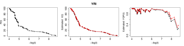
Figure 4: Discovery number $R(t)$, estimated false discovery number $V(t)$ and estimated false discovery proportion $\text{FDP}(t)$ as functions of a threshold on $t$ for populations CEU, JTPCHB and YRI. The $x$-axis is $-\log_{10}(t)$.

In the testing procedure by Fan et al. (2012b), a filtered least absolute deviation regression (LAD) is used to estimate the loading factors with $90\%$ of the cases (SNPs) whose test statistics are small and thus the resulting estimator is statistically biased. We upgrade this step with S.P described in Subsections 3.2 and 5.2 and re-estimate the number of false discoveries $V(t)$ and the false discovery proportion $\text{FDP}(t)$ as functions of $-\log_{10}(t)$, where $t$ is a thresholding value. Figure 4 shows the number of total discoveries $R(t)$, $\hat{V}(t)$ and $\widehat{\text{FDP}}(t)$ from procedures using filtered LAD and S.P. It is clear that $\hat{V}(t)$ and $\widehat{\text{FDP}}(t)$ with S.P are uniformly larger than but reasonably close to those with filtered LAD. Table 4 contains $R(t)$ and $\widehat{\text{FDP}}(t)$ with filtered LAD and S.P for several specific thresholds. The estimated FDPs with S.P for CEU and YRI are slightly larger than those with LAD and $\widehat{\text{FDP}}$ for JPTCHB with S.P is more than double of that with filtered LAD. This suggests that the estimation of FDP with filtered LAD might tend to be optimistic.

Population	$t$	$R(t)$	$\widehat{\text{FDP}}(t)$ with LAD	$\widehat{\text{FDP}}(t)$ with S.P
CEU	$6.12\times 10^{-4}$	4	.810	.845
JPTCHB	$1.51\times 10^{-9}$	5	.153	.373
YRI	$2.54\times 10^{-9}$	2	.227	.308

Table 4: Discovery numbers $R(t)$ and estimated false discover proportions $\hat{\text{FDP}}(t)$s from methods with LAD and S.P for specific values of threshold $t$.

6 Conclusion and Discussion

This paper considers the estimation of structural parameters with a finite or diverging number of covariates in a linear regression model with the presence of high-dimensional sparse incidental parameters. By exploiting the sparsity, we propose an estimation method penalizing the incidental parameters. The penalized estimator of the structural parameters is consistent and asymptotically Gaussian and achieves an oracle property. On the contrary, the penalized estimator of the incidental parameters possesses only partial selection consistency but not consistency. Thus, the structural parameters are consistently estimated while the incidental parameters not, which presents a partial consistency phenomenon. Further, in order to construct better confidence regions for the structural parameters, we propose a two-step estimator, which has fewer possible asymptotic distributions and can be asymptotically even more efficient than the one-step penalized estimator when the size and magnitude of nonzero incidental parameters are substantially large.

Simulation results show that the penalized methods with best regularization parameters achieve significantly smaller mean square errors than the ordinary least squares method which ignores the incidental parameters. Also provided is a data-driven regularization parameter, with which the penalized estimators continue to significantly outperform ordinary least squares when the incidental parameters are too large to be neglected. In terms of average length together with excellent coverage rates, the advantage of the confidence intervals based on the two-step estimator with an alternative data-driven regularization parameter is verified by simulations. A data set on genome-wide association is analyzed with a multiple testing procedure equipped with a data-driven penalized method and false discovery proportions are estimated.

In econometrics, a fixed effect panel data model is given by, for $1\leq i\leq n$ and $1\leq t\leq T$,

$$Y_{it}=\mu_{i}^{\star}+\boldsymbol{X}_{it}^{T}\boldsymbol{\beta}^{\star}+\epsilon_{it},$$ (6.1)

where $\mu_{i}^{\star}$’s are unknown fixed effects. When $T$ diverges, the fixed effects can be consistently estimated. When $T$ is finite and greater than or equal to 2, although the fixed effects can no longer be consistently estimated, they can be removed by a within-group transformation: for each $i$, $Y_{it}-\bar{Y}_{i}=(\boldsymbol{X}_{it}-\bar{\boldsymbol{X}}_{i})^{T}\boldsymbol{\beta}^{\star}+\epsilon_{it}-\bar{\epsilon}_{i}$, where $\bar{Y}_{i}$, $\bar{\boldsymbol{X}}_{i}$ and $\bar{\epsilon}_{i}$ are the averages of $Y_{it}$’s, $\boldsymbol{X}_{it}$’s and $\epsilon_{it}$’s, respectively. When $T$ is equal to 1, however, the within-group transformation fails. Note that, with $T=1$, Model (6.1) becomes Model (1.1) so that the proposed penalized estimations provide a solution under the sparsity assumption on the fixed effects.

Although this paper only illustrates the partial consistency phenomenon of a penalized estimation method for a linear regression model, such a phenomenon shall universally exist for a general parametric model, which contains both a structural parameter and a high-dimensional sparse incidental parameter. For example, consider a panel data logistic regression model: $P(Y_{it}=1|\boldsymbol{X}_{it})=(1+\exp\{-(\mu_{i}^{\star}+\boldsymbol{X}_{it}^{T}\boldsymbol{\beta}^{\star})\})^{-1}$. When $T$ is finite, the fixed effects $\mu_{i}^{\star}$’s cannot be removed by the within-group transformation as in the panel data linear model (6.1). However, the proposed penalized estimations can still provide a solution.

Further, if the structural parameter has a dimension diverging faster than the sample size and is sparse, it is expected that the partial consistency phenomenon will continue to appear when sparsity penalty is imposed on both the structural and incidental parameters.

Appendix A Appendix

In this appendix, we provide the proofs of the theoretical results in Section 4. The proofs of the results in Sections 2 and 3 are in Supplements D and E.

Denote $\mathbb{S}_{k,l}=\mathbb{S}_{\{k,k+1,\cdots,l\}}$ and $\mathbb{S}_{k,l}^{\epsilon}=\mathbb{S}_{\{k,k+1,\cdots,l\}}^{\epsilon}$. Let $\mathcal{B}=\{\max_{s+1\leq i\leq n}\lVert\boldsymbol{X}_{i}\rVert_{2}\leq\kappa_{n}\}$ and $\mathcal{D}=\bigcap_{i=1}^{n}\{-\gamma_{n}\leq\epsilon_{i}\leq\gamma_{n}\}$. Then $P(\mathcal{B})\rightarrow 1$ and $P(\mathcal{D})\rightarrow 1$ by (2.2).

A.1 Proof of Lemma 4.1

Proof of Lemma 4.1.

We first consider $S_{i0}$’s, then $S_{i1}$’s, and finally $S_{i2}$’s with $i=1,2,3$. Consider $S_{10}$, $S_{20}$ and $S_{30}$. Let $\mathcal{\mathcal{A}}=\{S_{10}=S_{10}^{\star}\}$. Note that $P(\mathcal{A})\geq P(\mathcal{A}|\mathcal{B})P(\mathcal{B})$ and $P(\mathcal{B})\rightarrow 1$. It suffices to show that $P(\mathcal{A}|\mathcal{B})\rightarrow 1$. By $\lambda\gg\sqrt{d}\kappa_{n}$, it follows $P(\mathcal{A}|\mathcal{B})\geq P(\{s+1\leq i\leq n:-\lambda+\max_{s+1\leq i\leq n}\lVert\boldsymbol{X}_{i}\rVert_{2}\sqrt{d}C\leq\epsilon_{i}\leq\lambda-\max_{s+1\leq i\leq n}\lVert\boldsymbol{X}_{i}\rVert_{2}\sqrt{d}C\}\supset S_{10}^{\star}|\mathcal{B})\geq P(\{s+1\leq i\leq n:-\lambda+\kappa_{n}\sqrt{d}C\leq\epsilon_{i}\leq\lambda-\kappa_{n}\sqrt{d}C\}\supset S_{10}^{\star})\geq P(\mathcal{D})\rightarrow 1$. Thus, wpg1, $S_{10}=S_{10}^{\star}$. From $S_{10}\cup S_{20}\cup S_{30}=S_{10}^{\star}$, it follows that, wpg1, $S_{20}=S_{30}=\emptyset$. Consider $S_{21}$, $S_{31}$ and $S_{11}$. Recall that $\mu^{\star}=\min\{|\mu_{i}^{\star}|:1\leq i\leq s_{1}\}$ and note that $\lambda-\mu^{\star}+\sqrt{d}C\kappa_{n}<-\gamma_{n}$ when $n$ is large. Let $S_{211}=S_{21}S_{21}^{\star}$ and $S_{212}=S_{21}S_{21}^{\star c}$. We will show $P(S_{211}=S_{21}^{\star})\rightarrow 1$ and $P(S_{212}=\emptyset)\rightarrow 1$. Then $P(S_{21}=S_{21}^{\star})\rightarrow 1$. Denote $\mathcal{A}_{1}=\{S_{211}\supset S_{21}^{\star}\}$. On the event $\mathcal{B}$, $S_{211}\supset\{1\leq i\leq s_{1}:\epsilon_{i}>\lambda-\mu^{\star}+\sqrt{d}C\kappa_{n}\text{ and }\mu_{i}^{\star}>0\}\supset\{1\leq i\leq s_{1}:\epsilon_{i}>-\gamma_{n}\text{ and }\mu_{i}^{\star}>0\}$. Then, $P(\mathcal{A}_{1})\geq P(\mathcal{A}_{1}|\mathcal{B})P(\mathcal{B})\geq P(\{1\leq i\leq s_{1}:\epsilon_{i}>-\gamma_{n}\text{ and }\mu_{i}^{\star}>0\}\supset S_{21}^{\star})P(\mathcal{B})\rightarrow 1\cdot 1=1$. It follows that, wpg1, $S_{211}\supset S_{21}^{\star}$. Note that $S_{211}\subset S_{21}^{\star}$. Then, wpg1, $S_{211}=S_{21}^{\star}$. Denote $\mathcal{A}_{2}=\{S_{212}=\emptyset\}$. On the event $\mathcal{B}$, $S_{212}\subset\{1\leq i\leq s_{1}:\epsilon_{i}>\lambda+\mu^{\star}-\sqrt{d}C\kappa_{n}\text{ and }\mu_{i}^{\star}<0\}$, which contains $\{1\leq i\leq s_{1}:\epsilon_{i}>\gamma_{n}\}$. Then, $P(\mathcal{A}_{2})\geq P(\mathcal{A}_{2}|\mathcal{B})P(\mathcal{B})\geq P(\{1\leq i\leq s_{1}:\epsilon_{i}>\gamma_{n}\}=\emptyset)P(\mathcal{B})\rightarrow=1$. Then, wpg1, $S_{212}=\emptyset$. Thus, $P(S_{21}=S_{21}^{\star})\rightarrow 1$. Similarly, we can show, wpg1, $S_{31}=S_{31}^{\star}$. Note that $S_{11}$, $S_{21}$ and $S_{31}$ are disjoint and their union is $S_{21}^{\star}\cup S_{31}^{\star}$. Then, wpg1, $S_{11}=\emptyset$. Consider $S_{12}$, $S_{22}$ and $S_{32}$. Denote $\mathcal{A}=\{S_{12}=S_{12}^{\star}\}$. Note that $-\lambda-\mu^{\star}_{i}+\sqrt{d}C\kappa_{n}<-\gamma_{n}$ and $\lambda-\mu^{\star}_{i}-\sqrt{d}C\kappa_{n}>\gamma_{n}$ when $n$ is large for $s_{1}+1\leq i\leq s$. On the event $\mathcal{B}$, $S_{12}\supset\{s_{1}+1\leq i\leq s:-\lambda-\mu^{\star}_{i}+\sqrt{d}C\kappa_{n}\leq\epsilon_{i}\leq\lambda-\mu^{\star}_{i}-\sqrt{d}C\kappa_{n}\}$, which contains $\{s_{1}+1\leq i\leq s:-\gamma_{n}\leq\epsilon_{i}\leq\gamma_{n}\}$. Then, $P(\mathcal{A})\geq P(\mathcal{A}|\mathcal{B})P(\mathcal{B})\geq P(\{s_{1}+1\leq i\leq s:-\gamma_{n}\leq\epsilon_{i}\leq\gamma_{n}\}=S_{12}^{\star})P(\mathcal{B})\rightarrow 1$. Thus, wpg1, $S_{12}=S_{12}^{\star}$. Note that $S_{12}$, $S_{22}$ and $S_{32}$ are disjoint and their union is $S_{12}^{\star}$. Then, wpg1, $S_{22}=S_{32}=\emptyset$. ∎

Before proceeding to the proofs of Theorems 4.2 to A.6, we denote $\bar{\sigma}_{X}^{2}=(1/d)\sum_{j=1}^{d}\text{Var}[X_{0j}]$ and $\bar{\sigma}_{XX}^{2}=(1/d^{2})\sum_{k=1}^{d}\sum_{l=1}^{d}\text{Var}[X_{0k}X_{0l}]$ and make the following assumptions.

Assumption (E1):

$\bar{\sigma}_{X}^{2}$ is bounded.

Assumption (E2):

$\bar{\sigma}_{XX}^{2}$ is bounded.

Assumption (E) in Section 4 implies Assumptions (E1) and (E2) by Cauchy-Schwarz inequality. For simplicity, we adopt the notation $\lesssim$, which means the left hand side is bounded by a constant times the right, where the constant does not affect related analysis.

A.2 Lemma A.2

Below are three lemmas needed for proving Theorems 4.2 to A.6. Their proofs are in Supplement F. Suppose that $\boldsymbol{M}$ and $\boldsymbol{E}$ are matrices and $\lVert\cdot\rVert$ is a matrix norm and that $\{\boldsymbol{A}_{n}\}$ is a sequence of random $d\times d$ matrices and $\boldsymbol{A}$ a deterministic $d\times d$ matrix, and denote $\hat{\boldsymbol{\Sigma}}_{n}=(1/n)\mathbb{S}_{n}$, the sample covariance matrix.

Lemma A.1 (Stewart (1969)).

If $\lVert\boldsymbol{I}\rVert=1$ and $\lVert\boldsymbol{M}^{-1}\rVert\lVert\boldsymbol{E}\rVert<1$, then

$$\frac{\lVert(\boldsymbol{M}+\boldsymbol{E})^{-1}-\boldsymbol{M}^{-1}\rVert}{\lVert\boldsymbol{M}^{-1}\rVert}\leq\frac{\lVert\boldsymbol{M}^{-1}\rVert\lVert\boldsymbol{E}\rVert}{1-\lVert\boldsymbol{M}^{-1}\rVert\lVert\boldsymbol{E}\rVert}.$$

Lemma A.2.

If $\lVert\boldsymbol{A}^{-1}\rVert_{F,d}$ is bounded, $\boldsymbol{A}_{n}\overset{P}{\longrightarrow}\boldsymbol{A}$, and $r_{d}\geq 1/\sqrt{d}$, then $\boldsymbol{A}_{n}^{-1}\overset{P}{\longrightarrow}\boldsymbol{A}^{-1}$, where the convergence in probability is wrt $r_{d}\lVert\cdot\rVert_{F}$.

A.3 Lemma A.3

Lemma A.3.

If Assumption (E2) holds and $r_{d}^{2}d^{4}/n\rightarrow 0$, then $\hat{\boldsymbol{\Sigma}}_{n}\overset{P}{\longrightarrow}\boldsymbol{\Sigma}_{X}$ wrt $r_{d}\lVert\cdot\rVert_{F}$.

Long Proof of Lemma A.3.

For any $\delta>0$, we have

$$P(\lVert\hat{\boldsymbol{\Sigma}}_{n}-\boldsymbol{\Sigma}\rVert_{F}>\delta)= P([\sum_{k=1}^{d}\sum_{l=1}^{d}(\frac{1}{n}\sum_{i=1}^{n}X_{ik}X_{il}-\sigma_{kl})^{2}]^{1/2}>\delta)$$

$$\leq \sum_{k=1}^{d}\sum_{l=1}^{d}P((\frac{1}{n}\sum_{i=1}^{n}X_{ik}X_{il}-\sigma_{kl})^{2}>\frac{\delta^{2}}{d^{2}})$$

$$\leq \sum_{k=1}^{d}\sum_{l=1}^{d}\frac{d^{2}}{\delta^{2}}P(\frac{1}{n}\sum_{i=1}^{n}X_{ik}X_{il}-\sigma_{kl})^{2}$$

$$= \sum_{k=1}^{d}\sum_{l=1}^{d}\frac{d^{2}}{\delta^{2}}\frac{1}{n^{2}}\sum_{i=1}^{n}P(X_{ik}X_{il}-\sigma_{kl})^{2}$$

$$= \sum_{k=1}^{d}\sum_{l=1}^{d}\frac{d^{2}}{\delta^{2}}\frac{1}{n^{2}}\sum_{i=1}^{n}P(X_{0k}X_{0l}-\sigma_{kl})^{2}$$

$$= \sum_{k=1}^{d}\sum_{l=1}^{d}\frac{d^{2}}{\delta^{2}}\frac{1}{n}\text{Var}[X_{0k}X_{0l}]$$

$$\leq \frac{d^{4}}{n}\frac{1}{\delta^{2}}\max_{1\leq k,l\leq d}\text{Var}[X_{0k}X_{0l}].$$

Thus, if $d^{4}/n\rightarrow 0$, then $\lVert\hat{\boldsymbol{\Sigma}}_{n}-\boldsymbol{\Sigma}\rVert_{F}\overset{P}{\longrightarrow}0$, which means that $\hat{\boldsymbol{\Sigma}}_{n}$ is a consistent estimator of $\boldsymbol{\Sigma}$ wrt $\lVert\cdot\rVert_{F}$.

Next, change $\delta$ to $\sqrt{d}\delta$. Then,

$$P(\lVert\hat{\boldsymbol{\Sigma}}_{n}-\boldsymbol{\Sigma}\rVert_{F,d}>\delta)\leq \frac{d^{4}}{n}\frac{1}{d\delta^{2}}\max_{1\leq k,l\leq d}\text{Var}[X_{0k}X_{0l}]$$

$$= \frac{d^{3}}{n}\frac{1}{\delta^{2}}\max_{1\leq k,l\leq d}\text{Var}[X_{0k}X_{0l}].$$

Thus, if $d^{3}/n\rightarrow 0$, then $\lVert\hat{\boldsymbol{\Sigma}}_{n}-\boldsymbol{\Sigma}\rVert_{F,d}\overset{P}{\longrightarrow}0$, which means that $\hat{\boldsymbol{\Sigma}}_{n}$ is a consistent estimator of $\boldsymbol{\Sigma}$ wrt $\lVert\cdot\rVert_{F,d}$. ∎

A.4 Proof of Theorem 4.2

Proof of Theorem 4.2.

By the proof of Lemma 4.1, wpg1, the solution $\hat{\boldsymbol{\beta}}_{n}$ to $\varphi_{n}(\boldsymbol{\beta})=0$ on $\mathcal{B}_{C}(\boldsymbol{\beta}^{\star})$ is explicitly given by $\hat{\boldsymbol{\beta}}_{n}=\boldsymbol{\beta}^{\star}+T_{0}^{-1}(T_{1}+T_{2}+T_{3}-T_{4})$, where $T_{0}=(1/n)\mathbb{S}_{s_{1}+1,n}$, $T_{1}=(1/n)\mathbb{S}_{S_{12}^{\star}}^{\mu}$, $T_{2}=(1/n)\mathbb{S}_{s_{1}+1,n}^{\epsilon}$, $T_{3}=(\lambda/n)\mathcal{S}_{S_{21}^{\star}}$ and $T_{4}=(\lambda/n)\mathcal{S}_{S_{31}^{\star}}$. Then, $r_{d}\lVert\hat{\boldsymbol{\beta}}_{n}-\boldsymbol{\beta}^{\star}\rVert_{2}\leq\lVert T_{0}^{-1}\rVert_{F,d}\sum_{i=1}^{4}r_{d}\sqrt{d}\lVert T_{i}\rVert_{2}.$ We will show that $\lVert T_{0}^{-1}\rVert_{F,d}$ is bounded by a positive constant wpg1 and $r_{d}\sqrt{d}\lVert T_{i}\rVert_{2}\overset{P}{\longrightarrow}0$ for $i=1,2,3,4$. Then, $r_{d}\lVert\hat{\boldsymbol{\beta}}_{n}-\boldsymbol{\beta}^{\star}\rVert_{2}=o_{P}(1)$. Consider $T_{0}$. By Lemma A.3, $\lVert T_{0}-\boldsymbol{\Sigma}_{X}\rVert_{F,d}\overset{P}{\longrightarrow}0$ under Assumption (E2) and the condition $d^{3}/n\rightarrow 0$. Then, by Lemma A.2, together with Assumption (D), $\lVert T_{0}^{-1}-\boldsymbol{\Sigma}_{X}^{-1}\rVert_{F,d}\overset{P}{\longrightarrow}0$. This implies that, wpg1, $\lVert T_{0}^{-1}\rVert_{F,d}$ is bounded by a positive constant. Consider $T_{1}$. Wpg1, $r_{d}\sqrt{d}\lVert T_{1}\rVert_{2}\leq r_{d}\sqrt{d}s_{2}\kappa_{n}\gamma_{n}/n=o(1)$ for $s_{2}=o(n/(r_{d}\sqrt{d}\kappa_{n}\gamma_{n}))$. Consider $T_{2}$. For any $\delta>0$, $P(\lVert T_{2}\rVert_{2}>\delta)\leq(1/\delta^{2})P\lVert(1/n)\sum_{i=s_{1}+1}^{n}\boldsymbol{X}_{i}\epsilon_{i}\rVert_{2}^{2}\leq d\sigma^{2}\bar{\sigma}_{X}^{2}/(n\delta^{2})$, where $\bar{\sigma}_{X}^{2}=(1/d)\sum_{j=1}^{d}\sigma_{j}^{2}$. Thus, $P(r_{d}\sqrt{d}\lVert T_{2}\rVert_{2}>\delta)\leq r_{d}^{2}d^{2}\sigma^{2}\bar{\sigma}_{X}^{2}/(n\delta^{2})\rightarrow 0$ by Assumption (E1) and $(r_{d}d)^{2}/n\rightarrow 0$. Consider $T_{3}$ and $T_{4}$. Wpg1, $r_{d}\sqrt{d}\lVert T_{3}\rVert_{2}\leq r_{d}\sqrt{d}\lambda s_{1}\kappa_{n}/n=o(1)$ for $s_{1}=o(n/(r_{d}\sqrt{d}\lambda\kappa_{n}))$. Similarly, $r_{d}\sqrt{d}\lVert T_{4}\rVert_{2}=o_{P}(1)$. ∎

Long Proof of Theorems 4.2.

By the proof of Theorem 3.2 and Lemma 3.1, wpg1, the solution $\hat{\boldsymbol{\beta}}_{n}$ to $\varphi_{n}(\boldsymbol{\beta})=0$ on $\mathcal{B}_{C}(\boldsymbol{\beta}^{\star})$ is explicitly given by

$$\hat{\boldsymbol{\beta}}_{n}=\boldsymbol{\beta}^{\star}+T_{0}^{-1}(T_{1}+T_{2}+T_{3}-T_{4}),$$

where

$$T_{0} =(1/n)\mathbb{S}_{s_{1}+1,n},$$

$$T_{1} =(1/n)\mathbb{S}_{S_{12}^{\star}}^{\mu},$$

$$T_{2} =(1/n)\mathbb{S}_{s_{1}+1,n}^{\epsilon},$$

$$T_{3} =(\lambda/n)\mathcal{S}_{S_{21}^{\star}},$$

$$T_{4} =(\lambda/n)\mathcal{S}_{S_{31}^{\star}}.$$

Then,

$$\lVert\hat{\boldsymbol{\beta}}_{n}-\boldsymbol{\beta}^{\star}\rVert_{2} \leq\lVert T_{0}^{-1}(T_{1}+T_{2}+T_{3}-T_{4})\rVert_{2}$$

$$\leq\lVert T_{0}^{-1}\rVert_{F}\lVert T_{1}+T_{2}+T_{3}-T_{4})\rVert_{2}$$

$$\leq\lVert T_{0}^{-1}\rVert_{F}\sum_{i=1}^{4}\lVert T_{i}\rVert_{2}.$$

Then,

$$r_{d}\lVert\hat{\boldsymbol{\beta}}_{n}-\boldsymbol{\beta}^{\star}\rVert_{2} \leq\frac{1}{\sqrt{d}}\lVert T_{0}^{-1}\rVert_{F}\sum_{i=1}^{4}r_{d}\sqrt{d}\lVert T_{i}\rVert_{2}.$$

We will show the followings:

• $(1/\sqrt{d})\lVert T_{0}^{-1}\rVert_{F}$ is bounded by a constant wpg1.

• $r_{d}\sqrt{d}\lVert T_{i}\rVert_{2}\overset{P}{\longrightarrow}0$ for $i=1,2,3,4$.

Thus, we have the following conclusions:

• $r_{d}\lVert\hat{\boldsymbol{\beta}}_{n}-\boldsymbol{\beta}^{\star}\rVert_{2}=o_{P}(1)$, that is, $\lVert\hat{\boldsymbol{\beta}}_{n}-\boldsymbol{\beta}^{\star}\rVert_{2}=o_{P}(1/r_{d})$.

On $(1/\sqrt{d})\lVert T_{0}^{-1}\rVert_{F}$. We will show that

$$(1/\sqrt{d})\lVert T_{0}^{-1}\rVert_{F}-(1/\sqrt{d})\lVert\boldsymbol{\Sigma}_{X}^{-1}\rVert_{F}\overset{P}{\longrightarrow}0.$$

By the assumption that there exists a constant $C>0$ such that

$$(1/\sqrt{d})\lVert\boldsymbol{\Sigma}_{X}^{-1}\rVert_{F}\leq C,$$

we have, wpg1,

$$(1/\sqrt{d})\lVert T_{0}^{-1}\rVert_{F}\leq 2C.$$

Since

$$|\lVert T_{0}^{-1}\rVert_{F,d}-\lVert\boldsymbol{\Sigma}_{X}^{-1}\rVert_{F,d}|\leq\lVert T_{0}^{-1}-\boldsymbol{\Sigma}_{X}^{-1}\rVert_{F,d},$$

it is sufficient to show that

$$\lVert T_{0}^{-1}-\boldsymbol{\Sigma}_{X}^{-1}\rVert_{F,d}\overset{P}{\longrightarrow}0.$$

By Lemma A.2, it is sufficient to show that

$$\lVert T_{0}-\boldsymbol{\Sigma}_{X}\rVert_{F,d}\overset{P}{\longrightarrow}0.$$

In fact, by Lemma A.3, this holds under the condition that $d^{3}/n\rightarrow 0$.

Thus, wpg1, $\lVert T_{0}^{-1}\rVert_{F,d}$ is bounded by a constant under the conditions

• There exists a constant $C>0$ such that $\lVert\boldsymbol{\Sigma}_{X}^{-1}\rVert_{F,d}\leq C$.

• $d^{3}/n\rightarrow 0$.

On $T_{1}$. We have, wpg1,

$$r_{d}\sqrt{d}\lVert T_{1}\rVert_{2} \leq r_{d}\sqrt{d}\frac{1}{n}\sum_{i=s_{1}+1}^{s}\lVert\boldsymbol{X}_{i}\mu_{i}^{\star}\rVert_{2}$$

$$=r_{d}\sqrt{d}\frac{1}{n}\sum_{i=s_{1}+1}^{s}\lVert\boldsymbol{X}_{i}\rVert_{2}\cdot|\mu_{i}^{\star}|$$

$$\leq r_{d}\sqrt{d}s_{2}\kappa_{n}\gamma_{n}/n.$$

Thus, if $s_{2}=o(n/(r_{d}\sqrt{d}\kappa_{n}\gamma_{n}))$, then $r_{d}\sqrt{d}\lVert T_{1}\rVert_{2}=o_{P}(1)$.

On $T_{2}$. We have

$$T_{2} =(1/n)\mathbb{S}_{s_{1}+1,n}^{\epsilon}=(1/n)\sum_{i=s_{1}+1}^{n}\boldsymbol{X}_{i}^{T}\epsilon_{i}.$$

We have

$$P(\lVert T_{2}\rVert_{2}>\delta) =P(\lVert(1/n)\sum_{i=s_{1}+1}^{n}\boldsymbol{X}_{i}\epsilon_{i}\rVert_{2}>\delta)$$

$$\leq\frac{1}{\delta^{2}}P\lVert(1/n)\sum_{i=s_{1}+1}^{n}\boldsymbol{X}_{i}\epsilon_{i}\rVert_{2}^{2}$$

$$=\frac{1}{\delta^{2}}\frac{1}{n^{2}}P\lVert\sum_{i=s_{1}+1}^{n}\boldsymbol{X}_{i}\epsilon_{i}\rVert_{2}^{2}$$

$$=\frac{1}{\delta^{2}}\frac{1}{n^{2}}P\sum_{i=s_{1}+1}^{n}\sum_{j=s_{1}+1}^{n}\boldsymbol{X}_{i}^{T}\boldsymbol{X}_{j}\epsilon_{i}\epsilon_{j}$$

$$=\frac{1}{\delta^{2}}\frac{1}{n^{2}}\sum_{i=s_{1}+1}^{n}P\lVert\boldsymbol{X}_{i}\rVert_{2}^{2}\epsilon_{i}^{2}$$

$$=\frac{1}{\delta^{2}}\frac{1}{n^{2}}\sum_{i=s_{1}+1}^{n}P\lVert\boldsymbol{X}_{i}\rVert_{2}^{2}P\epsilon_{i}^{2}$$

$$=\frac{1}{\delta^{2}}\frac{1}{n^{2}}(n-s_{1})P\lVert\boldsymbol{X}_{0}\rVert_{2}^{2}P\epsilon_{0}^{2}$$

$$=\frac{1}{\delta^{2}}\frac{1}{n^{2}}(n-s_{1})P\lVert\boldsymbol{X}_{0}\rVert_{2}^{2}\sigma^{2}$$

$$=\frac{1}{\delta^{2}}\frac{1}{n^{2}}(n-s_{1})\sigma^{2}\sum_{j=1}^{d}PX_{0j}^{2}$$

$$=\frac{1}{\delta^{2}}\frac{1}{n^{2}}(n-s_{1})\sigma^{2}\sum_{j=1}^{d}\sigma_{j}^{2}$$

$$=\frac{1}{\delta^{2}}\frac{1}{n^{2}}d(n-s_{1})\sigma^{2}\frac{1}{d}\sum_{j=1}^{d}\sigma_{j}^{2}$$

$$\leq\frac{1}{\delta^{2}}\frac{d}{n}\sigma^{2}\frac{1}{d}\sum_{j=1}^{d}\sigma_{j}^{2}$$

$$\leq\frac{1}{\delta^{2}}\frac{d}{n}\sigma^{2}\sigma_{X}^{2},$$

where $\sigma_{X}^{2}=\max_{1\leq j\leq d}\sigma_{j}^{2}$ is bounded. Thus, we have

$$P(r_{d}\sqrt{d}\lVert T_{2}\rVert_{2}>\delta)\leq\frac{1}{\delta^{2}}\frac{(r_{d}d)^{2}}{n}\sigma^{2}\sigma_{X}^{2}.$$

Thus, if $(r_{d}d)^{2}/n\rightarrow 0$, then $r_{d}\sqrt{d}\lVert T_{2}\rVert_{2}\overset{P}{\longrightarrow}0$.

On $T_{3}$ and $T_{4}$. We have, wpg1,

$$r_{d}\sqrt{d}\lVert T_{3}\rVert_{2} =r_{d}\sqrt{d}\lVert\lambda\frac{1}{n}\mathcal{S}_{S_{21}^{\star}}\rVert_{2}$$

$$=r_{d}\sqrt{d}\lambda\frac{1}{n}\lVert\mathcal{S}_{S_{21}^{\star}}\rVert_{2}$$

$$\leq r_{d}\sqrt{d}\lambda\frac{1}{n}\#(S_{21}^{\star})\kappa_{n}$$

$$\leq r_{d}\sqrt{d}\lambda s_{1}\kappa_{n}/n.$$

Thus, if $s_{1}=o(n/(r_{d}\sqrt{d}\lambda\kappa_{n}))$, then $r_{d}\sqrt{d}\lVert T_{3}\rVert_{2}=o_{P}(1)$. In the same way, we can show that $r_{d}\sqrt{d}\lVert T_{4}\rVert_{2}=o_{P}(1)$ under the condition $s_{1}=o(n/(r_{d}\sqrt{d}\lambda\kappa_{n}))$.

Therefore, $\hat{\boldsymbol{\beta}}_{n}$ is a consistent estimator of $\boldsymbol{\beta}^{\star}$ wrt $r_{d}\lVert\cdot\rVert_{2,d}$.

Next, we show some special cases with $r_{d}=1$ and $r_{d}=1/\sqrt{d}$. We have,

$$\lVert\hat{\boldsymbol{\beta}}_{n}-\boldsymbol{\beta}^{\star}\rVert_{2} \leq\lVert T_{0}^{-1}(T_{1}+T_{2}+T_{3}-T_{4})\rVert_{2}$$

$$\leq\lVert T_{0}^{-1}\rVert_{F}\lVert T_{1}+T_{2}+T_{3}-T_{4})\rVert_{2}$$

$$\leq\lVert T_{0}^{-1}\rVert_{F}\sum_{i=1}^{4}\lVert T_{i}\rVert_{2}.$$

Then,

$$\frac{1}{\sqrt{d}}\lVert\hat{\boldsymbol{\beta}}_{n}-\boldsymbol{\beta}^{\star}\rVert_{2} \leq\frac{1}{\sqrt{d}}\lVert T_{0}^{-1}\rVert_{F}\sum_{i=1}^{4}\lVert T_{i}\rVert_{2}.$$

We will show the followings:

• $(1/\sqrt{d})\lVert T_{0}^{-1}\rVert_{F}$ is bounded by a constant wpg1.

• $\lVert T_{i}\rVert_{2}\overset{P}{\longrightarrow}0$ for $i=1,2,3,4$.

• $\sqrt{d}\lVert T_{i}\rVert_{2}\overset{P}{\longrightarrow}0$ for $i=1,2,3,4$.

Thus, we have the following conclusions:

• $(1/\sqrt{d})\lVert\hat{\boldsymbol{\beta}}_{n}-\boldsymbol{\beta}^{\star}\rVert_{2}=o_{P}(1)$, that is, $\lVert\hat{\boldsymbol{\beta}}_{n}-\boldsymbol{\beta}^{\star}\rVert_{2}=o_{P}(\sqrt{d})$.

• $\lVert\hat{\boldsymbol{\beta}}_{n}-\boldsymbol{\beta}^{\star}\rVert_{2}=o_{P}(1)$, that is, $\lVert\hat{\boldsymbol{\beta}}_{n}-\boldsymbol{\beta}^{\star}\rVert_{2}=o_{P}(1)$.

On $(1/\sqrt{d})\lVert T_{0}^{-1}\rVert_{F}$. We will show that

$$(1/\sqrt{d})\lVert T_{0}^{-1}\rVert_{F}-(1/\sqrt{d})\lVert\boldsymbol{\Sigma}_{X}^{-1}\rVert_{F}\overset{P}{\longrightarrow}0.$$

By the assumption that there exists a constant $C>0$ such that

$$(1/\sqrt{d})\lVert\boldsymbol{\Sigma}_{X}^{-1}\rVert_{F}\leq C,$$

we have, wpg1,

$$(1/\sqrt{d})\lVert T_{0}^{-1}\rVert_{F}\leq 2C.$$

Since

$$|\lVert T_{0}^{-1}\rVert_{F,d}-\lVert\boldsymbol{\Sigma}_{X}^{-1}\rVert_{F,d}|\leq\lVert T_{0}^{-1}-\boldsymbol{\Sigma}_{X}^{-1}\rVert_{F,d},$$

it is sufficient to show that

$$\lVert T_{0}^{-1}-\boldsymbol{\Sigma}_{X}^{-1}\rVert_{F,d}\overset{P}{\longrightarrow}0.$$

By Lemma A.2, it is sufficient to show that

$$\lVert T_{0}-\boldsymbol{\Sigma}_{X}\rVert_{F,d}\overset{P}{\longrightarrow}0.$$

In fact, by Lemma A.3, this holds under the condition that $d^{3}/n\rightarrow 0$.

Thus, wpg1, $\lVert T_{0}^{-1}\rVert_{F,d}$ is bounded by a constant under the conditions

• There exists a constant $C>0$ such that $\lVert\boldsymbol{\Sigma}_{X}^{-1}\rVert_{F,d}\leq C$.

• $d^{3}/n\rightarrow 0$.

On $T_{1}$. We have, wpg1,

$$\lVert T_{1}\rVert_{2} \leq\frac{1}{n}\sum_{i=s_{1}+1}^{s}\lVert\boldsymbol{X}_{i}\mu_{i}^{\star}\rVert_{2}=\frac{1}{n}\sum_{i=s_{1}+1}^{s}\lVert\boldsymbol{X}_{i}\rVert_{2}\cdot|\mu_{i}^{\star}|\leq s_{2}\kappa_{n}\gamma_{n}/n.$$

Thus, if $s_{2}=o(n/(\kappa_{n}\gamma_{n}))$, then $\lVert T_{1}\rVert_{2}=o_{P}(1)$.

Similarly, we have

$$\sqrt{d}\lVert T_{1}\rVert_{2}\leq s_{2}\kappa_{n}\gamma_{n}\sqrt{d}/n.$$

Thus, if $s_{2}=o(n/(\sqrt{d}\kappa_{n}\gamma_{n}))$, then $\sqrt{d}\lVert T_{1}\rVert_{2}=o_{P}(1)$.

On $T_{2}$. We have

$$T_{2} =(1/n)\mathbb{S}_{s_{1}+1,n}^{\epsilon}=(1/n)\sum_{i=s_{1}+1}^{n}\boldsymbol{X}_{i}^{T}\epsilon_{i}.$$

We have

$$P(\lVert T_{2}\rVert_{2}>\delta) =P(\lVert(1/n)\sum_{i=s_{1}+1}^{n}\boldsymbol{X}_{i}\epsilon_{i}\rVert_{2}>\delta)$$

$$\leq\frac{1}{\delta^{2}}P\lVert(1/n)\sum_{i=s_{1}+1}^{n}\boldsymbol{X}_{i}\epsilon_{i}\rVert_{2}^{2}$$

$$=\frac{1}{\delta^{2}}\frac{1}{n^{2}}P\lVert\sum_{i=s_{1}+1}^{n}\boldsymbol{X}_{i}\epsilon_{i}\rVert_{2}^{2}$$

$$=\frac{1}{\delta^{2}}\frac{1}{n^{2}}P\sum_{i=s_{1}+1}^{n}\sum_{j=s_{1}+1}^{n}\boldsymbol{X}_{i}^{T}\boldsymbol{X}_{j}\epsilon_{i}\epsilon_{j}$$

$$=\frac{1}{\delta^{2}}\frac{1}{n^{2}}\sum_{i=s_{1}+1}^{n}P\lVert\boldsymbol{X}_{i}\rVert_{2}^{2}\epsilon_{i}^{2}$$

$$=\frac{1}{\delta^{2}}\frac{1}{n^{2}}\sum_{i=s_{1}+1}^{n}P\lVert\boldsymbol{X}_{i}\rVert_{2}^{2}P\epsilon_{i}^{2}$$

$$=\frac{1}{\delta^{2}}\frac{1}{n^{2}}(n-s_{1})P\lVert\boldsymbol{X}_{0}\rVert_{2}^{2}P\epsilon_{0}^{2}$$

$$=\frac{1}{\delta^{2}}\frac{1}{n^{2}}(n-s_{1})P\lVert\boldsymbol{X}_{0}\rVert_{2}^{2}\sigma^{2}$$

$$=\frac{1}{\delta^{2}}\frac{1}{n^{2}}(n-s_{1})\sigma^{2}\sum_{j=1}^{d}PX_{0j}^{2}$$

$$=\frac{1}{\delta^{2}}\frac{1}{n^{2}}(n-s_{1})\sigma^{2}\sum_{j=1}^{d}\sigma_{j}^{2}$$

$$=\frac{1}{\delta^{2}}\frac{1}{n^{2}}d(n-s_{1})\sigma^{2}\frac{1}{d}\sum_{j=1}^{d}\sigma_{j}^{2}$$

$$\leq\frac{1}{\delta^{2}}\frac{d}{n}\sigma^{2}\frac{1}{d}\sum_{j=1}^{d}\sigma_{j}^{2}$$

$$\leq\frac{1}{\delta^{2}}\frac{d}{n}\sigma^{2}\sigma_{X}^{2},$$

where $\sigma_{X}^{2}=\max_{1\leq j\leq d}\sigma_{j}^{2}$ is bounded. Thus, if $d/n\rightarrow 0$, then $\lVert T_{2}\rVert_{2}\overset{P}{\longrightarrow}0$.

From the above derivation, we have

$$P(\sqrt{d}\lVert T_{2}\rVert_{2}>\delta)\leq\frac{1}{\delta^{2}}\frac{d^{2}}{n}\sigma^{2}\sigma_{X}^{2}.$$

Thus, if $d^{2}/n\rightarrow 0$, then $\sqrt{d}\lVert T_{2}\rVert_{2}\overset{P}{\longrightarrow}0$.

On $T_{3}$ and $T_{4}$. We have, wpg1,

$$\lVert T_{3}\rVert_{2}=\lVert\lambda\frac{1}{n}\mathcal{S}_{S_{21}^{\star}}\rVert_{2}=\lambda\frac{1}{n}\lVert\mathcal{S}_{S_{21}^{\star}}\rVert_{2}\leq\lambda\frac{1}{n}\#(S_{21}^{\star})\kappa_{n}\leq\lambda s_{1}\kappa_{n}/n.$$

Thus, if $s_{1}=o(n/(\lambda\kappa_{n}))$, then $T_{3}=o_{P}(1)$. In the same way, we can show that $T_{4}=o_{P}(1)$ under the condition $s_{1}=o(n/(\lambda\kappa_{n}))$.

From the above derivation, we have

$$\sqrt{d}\lVert T_{3}\rVert_{2}\leq\lambda s_{1}\kappa_{n}\sqrt{d}/n.$$

Thus, if $s_{1}=o(n/(\sqrt{d}\lambda\kappa_{n}))$, then $T_{3}=o_{P}(1)$. In the same way, we can show that $T_{4}=o_{P}(1)$ under the condition $s_{1}=o(n/(\sqrt{d}\lambda\kappa_{n}))$.

Therefore, $\hat{\boldsymbol{\beta}}_{n}$ is a consistent estimator of $\boldsymbol{\beta}^{\star}$ wrt $\lVert\cdot\rVert_{2,d}$. ∎

A.5 Lemma A.4

The next lemma is needed for proving Theorem 4.3 and its proof is in Supplement F. Suppose $\{\boldsymbol{\xi}_{i}\}$ are i.i.d. copies of $\boldsymbol{\xi}_{0}$, a $d$-dimensional random vector with mean zero. Denote $\sigma_{\xi,\max}^{2}=\max_{1\leq j\leq d}\text{Var}[\xi_{0j}]$, $\sigma_{\xi,\min}^{2}=\min_{1\leq j\leq d}\text{Var}[\xi_{0j}]$ and $\gamma_{\xi,\max}=\max_{1\leq j\leq d}\mathbb{E}|\xi_{0j}|^{3}$.

Lemma A.4.

Suppose $\sigma_{\xi,\max}$ and $\gamma_{\xi,\max}$ are bounded from above and $\sigma_{\xi,\max}$ is bounded from zero. If $d=o(\sqrt{n})$, then $(1/\sqrt{n})\sum_{i=1}^{n}\boldsymbol{\xi}_{i}=O_{P}(\sqrt{d\log{d}})$ wrt $\lVert\cdot\rVert_{2}$.

A.6 Proof of Theorem 4.3

Proof of Theorem 4.3.

We reuse the notations $T_{i}$’s in the proof of Theorems 4.2, from which, $\sqrt{n}\boldsymbol{A}_{n}(\hat{\boldsymbol{\beta}}_{n}-\boldsymbol{\beta}^{\star})=V_{1}+V_{2}+V_{3}-V_{4}$, where $V_{i}=\boldsymbol{B}_{n}T_{i}$ for $i=1,2,3,4$ and $\boldsymbol{B}_{n}=\sqrt{n}\boldsymbol{A}_{n}T_{0}^{-1}$. It is sufficient to show that $V_{2}\overset{d}{\longrightarrow}N(0,\sigma^{2}\boldsymbol{G}_{X})$ and other $V_{i}$’s are $o_{P}(1)$. Consider $V_{1}$. We have $\lVert V_{1}\rVert_{2}\leq\sqrt{nd}\lVert\boldsymbol{A}_{n}\rVert_{F}\lVert T_{0}^{-1}\rVert_{F,d}\lVert T_{1}\rVert_{2}.$ By Assumption (F), $\lVert\boldsymbol{A}_{n}\rVert_{F}$ is bounded. By Lemmas A.2 and A.3 and Assumption (D), for $d=o(n^{1/3})$, wpg1, $\lVert T_{0}^{-1}\rVert_{F,d}$ is bounded. We have, wpg1, $\lVert T_{1}\rVert_{2}\leq s_{2}\kappa_{n}\gamma_{n}/n$. Then, $\lVert V_{1}\rVert_{2}\lesssim\sqrt{d/n}s_{2}\kappa_{n}\gamma_{n},$ Thus, $\lVert V_{1}\rVert_{2}=o_{P}(1)$ for $s_{2}=o(\sqrt{n}/(\sqrt{d}\kappa_{n}\gamma_{n}))$. Consider $V_{2}$. We have $V_{2}=V_{21}+V_{22}$, where $V_{21}=\sqrt{n}\boldsymbol{A}_{n}\boldsymbol{\boldsymbol{\Sigma}}_{X}^{-1}T_{2}$ and $V_{22}=\sqrt{n}\boldsymbol{A}_{n}(T_{0}^{-1}-\boldsymbol{\boldsymbol{\Sigma}}_{X}^{-1})T_{2}$. First, note that $V_{21}=\sqrt{(n-s_{1})/n}\sum_{i=s_{1}+1}^{n}\boldsymbol{Z}_{n,i}$, where $\boldsymbol{Z}_{n,i}=(1/\sqrt{n-s_{1}})\boldsymbol{A}_{n}\boldsymbol{\boldsymbol{\Sigma}}_{X}^{-1}\boldsymbol{X}_{i}\epsilon_{i}$. On one hand, for every $\delta>0$, $\sum_{i=s_{1}+1}^{n}\mathbb{E}\lVert\boldsymbol{Z}_{n,i}\rVert_{2}^{2}\{\lVert\boldsymbol{Z}_{n,i}\rVert_{2}>\delta\}\leq(n-s_{1})\mathbb{E}\lVert\boldsymbol{Z}_{n,0}\rVert_{2}^{4}/\delta^{2},$ and $\mathbb{E}\lVert\boldsymbol{Z}_{n,0}\rVert_{2}^{4}=\frac{1}{(n-s_{1})^{2}}\mathbb{E}\epsilon_{0}^{4}\mathbb{E}(\boldsymbol{X}_{0}^{T}\boldsymbol{\boldsymbol{\Sigma}}_{X}^{-1}\boldsymbol{A}_{n}^{T}\boldsymbol{A}_{n}\boldsymbol{\boldsymbol{\Sigma}}_{X}^{-1}\boldsymbol{X}_{0})^{2}$, which is $\leq\frac{d^{2}}{(n-s_{1})^{2}}\mathbb{E}\epsilon_{0}^{4}\lambda_{\max}(\boldsymbol{G}_{n})\lambda_{\min}^{-2}(\boldsymbol{\boldsymbol{\Sigma}}_{X})\kappa_{X}^{2}$. Then, by Assumptions (D’), (E) and (F) and for $d=o(\sqrt{n})$, $\sum_{i=s_{1}+1}^{n}\mathbb{E}\lVert\boldsymbol{Z}_{n,i}\rVert_{2}^{2}\{\lVert\boldsymbol{Z}_{n,i}\rVert_{2}>\delta\}\rightarrow 0$. On the other hand, $\sum_{i=s_{1}+1}^{n}\text{Cov}(\boldsymbol{Z}_{n,i})=\sigma^{2}\boldsymbol{A}_{n}\boldsymbol{\boldsymbol{\Sigma}}_{X}^{-1}\boldsymbol{A}_{n}^{T}\rightarrow\sigma^{2}\boldsymbol{G}_{X}$ by Assumption (F). Thus, by central limit theorem (see Proposition 2.27 in van der Vaart (1998)), $V_{21}\overset{d}{\longrightarrow}N(0,\sigma^{2}\boldsymbol{G}_{X})$. Next, consider $V_{22}$. Note that $\lVert V_{22}\rVert_{2}\leq\lVert\boldsymbol{A}_{n}\rVert_{F}(d\log(d))^{1/2}\lVert T_{0}^{-1}-\boldsymbol{\boldsymbol{\Sigma}}_{X}^{-1}\rVert_{F}(d\log(d))^{-1/2}\lVert\sqrt{n}T_{2}\rVert_{2}$. By Assumption (F), $\lVert\boldsymbol{A}_{n}\rVert_{F}$ is $O(1)$; by Lemmas A.2 and A.3, $(d\log(d))^{1/2}\lVert T_{0}^{-1}-\boldsymbol{\boldsymbol{\Sigma}}_{X}^{-1}\rVert_{F}$ is $o_{P}(1)$ for $d^{5}\log(d)=o(n)$; by Lemma A.4, $(d\log(d))^{-1/2}\lVert\sqrt{n}T_{2}\rVert_{2}=(d\log(d))^{-1/2}\lVert\frac{1}{\sqrt{n}}\mathbb{S}_{s_{1}+1,n}^{\epsilon}\rVert_{2}$ is $O_{P}(1)$ for $d=o(\sqrt{n})$. Then, $V_{22}\overset{P}{\longrightarrow}0$. Thus, by slutsky’s lemma, $V_{2}\overset{d}{\longrightarrow}N(0,\sigma^{2}\boldsymbol{G}_{X})$. Consider $V_{3}$ and $V_{4}$. First consider $V_{3}$. By noting that $s_{1}=o(\sqrt{n}/(\lambda\sqrt{d}\kappa_{n}))$, wpg1, $\lVert V_{3}\rVert_{2}\leq\sqrt{nd}\lVert\boldsymbol{A}_{n}\rVert_{F}\lVert T_{0}^{-1}\rVert_{F,d}\lVert T_{3}\rVert_{2}\lesssim\sqrt{d}\lambda s_{1}\kappa_{n}/\sqrt{n}\rightarrow 0$. Thus, $\lVert V_{3}\rVert_{2}=o_{P}(1)$. In the same way, $\lVert V_{4}\rVert_{2}=o_{P}(1)$. ∎

Long Proof of Theorem 4.3.

We reuse the notations on $T_{i}$’s in the proof of Theorems 4.2, from which,

$$\sqrt{n}\boldsymbol{A}_{n}(\hat{\boldsymbol{\beta}}_{n}-\boldsymbol{\beta}^{\star})=V_{1}+V_{2}+V_{3}-V_{4},$$

where

$$V_{1} =\sqrt{n}\boldsymbol{A}_{n}T_{0}^{-1}T_{1},$$

$$V_{2} =\sqrt{n}\boldsymbol{A}_{n}T_{0}^{-1}T_{2},$$

$$V_{3} =\sqrt{n}\boldsymbol{A}_{n}T_{0}^{-1}T_{3},$$

$$V_{4} =\sqrt{n}\boldsymbol{A}_{n}T_{0}^{-1}T_{4}.$$

Next we derive the asymptotic properties of $V_{i}$’s, from which the desired result follows by applying Slutsky’s lemma.

On $V_{1}$. We have

$$\lVert V_{1}\rVert_{2} =\lVert\sqrt{n}T_{0}^{-1}T_{1}\rVert_{2}$$

$$\leq\sqrt{n}\lVert\boldsymbol{A}_{n}\rVert_{F}\lVert T_{0}^{-1}\rVert_{F}\lVert T_{1}\rVert_{2}$$

$$=\sqrt{nd}\lVert\boldsymbol{A}_{n}\rVert_{F}\lVert T_{0}^{-1}\rVert_{F,d}\lVert T_{1}\rVert_{2}.$$

By Assumption (F) $\lVert\boldsymbol{A}_{n}\rVert_{F}$ is bounded.

By Lemmas A.2 and A.3 and Assumption (D), for $d=o(n^{1/3})$, wpg1, $\lVert T_{0}^{-1}\rVert_{F,d}$ is bounded.

We have, wpg1,

$$\lVert T_{1}\rVert_{2}=\lVert\frac{1}{n}\sum_{i=s_{1}+1}^{s}\boldsymbol{X}_{i}\mu_{i}^{\star}\rVert_{2}\leq\frac{1}{n}s_{2}\kappa_{n}\gamma_{n}.$$

Then,

$$\lVert V_{1}\rVert_{2} \lesssim\sqrt{\frac{d}{n}}s_{2}\kappa_{n}\gamma_{n},$$

where $\lesssim$ means that the left side is bounded by a constant times the right side.

Thus, $\lVert V_{1}\rVert_{2}=o_{P}(1)$ for $s_{2}=o(\sqrt{n}/(\sqrt{d}\kappa_{n}\gamma_{n}))$.

On $V_{2}$. We have $V_{2}=V_{21}+V_{22}$, where

$$V_{21} =\sqrt{n}\boldsymbol{A}_{n}\boldsymbol{\boldsymbol{\Sigma}}_{X}^{-1}T_{2},$$

$$V_{22} =\sqrt{n}\boldsymbol{A}_{n}(T_{0}^{-1}-\boldsymbol{\boldsymbol{\Sigma}}_{X}^{-1})T_{2}.$$

First, consider $V_{21}$. We have

$$V_{21} =\sqrt{n}\boldsymbol{A}_{n}\boldsymbol{\boldsymbol{\Sigma}}_{X}^{-1}T_{2}$$

$$=\sqrt{n}\boldsymbol{A}_{n}\boldsymbol{\boldsymbol{\Sigma}}_{X}^{-1}\frac{1}{n}\sum_{i=s_{1}+1}^{n}\boldsymbol{X}_{i}\epsilon_{i}$$

$$=\frac{\sqrt{n-s_{1}}}{\sqrt{n}}\sum_{i=s_{1}+1}^{n}\boldsymbol{Z}_{n,i},$$

where

$$\boldsymbol{Z}_{n,i}=\frac{1}{\sqrt{n-s_{1}}}\boldsymbol{A}_{n}\boldsymbol{\boldsymbol{\Sigma}}_{X}^{-1}\boldsymbol{X}_{i}\epsilon_{i}.$$

For every $\delta>0$,

$$\sum_{i=s_{1}+1}^{n}\mathbb{E}\lVert\boldsymbol{Z}_{n,i}\rVert_{2}^{2}\{\lVert\boldsymbol{Z}_{n,i}\rVert_{2}>\delta\} \leq\sum_{i=s_{1}+1}^{n}\mathbb{E}\lVert\boldsymbol{Z}_{n,i}\rVert_{2}^{4}/\delta^{2}=(n-s_{1})\mathbb{E}\lVert\boldsymbol{Z}_{n,0}\rVert_{2}^{4}/\delta^{2},$$

and

$$\mathbb{E}\lVert\boldsymbol{Z}_{n,0}\rVert_{2}^{4} =\mathbb{E}(\lVert\boldsymbol{Z}_{n,0}\rVert_{2}^{2})^{2}$$

$$=\mathbb{E}(\frac{1}{n-s_{1}}\epsilon_{0}^{2}\boldsymbol{X}_{0}^{T}\boldsymbol{\boldsymbol{\Sigma}}_{X}^{-1}\boldsymbol{A}_{n}^{T}\boldsymbol{A}_{n}\boldsymbol{\boldsymbol{\Sigma}}_{X}^{-1}\boldsymbol{X}_{0})^{2}$$

$$=\frac{1}{(n-s_{1})^{2}}\mathbb{E}\epsilon_{0}^{4}\mathbb{E}(\boldsymbol{X}_{0}^{T}\boldsymbol{\boldsymbol{\Sigma}}_{X}^{-1}\boldsymbol{A}_{n}^{T}\boldsymbol{A}_{n}\boldsymbol{\boldsymbol{\Sigma}}_{X}^{-1}\boldsymbol{X}_{0})^{2}$$

$$\leq\frac{1}{(n-s_{1})^{2}}\mathbb{E}\epsilon_{0}^{4}\lambda_{\max}(\boldsymbol{G}_{n})\lambda_{\min}(\boldsymbol{\boldsymbol{\Sigma}}_{X})^{-2}\mathbb{E}(\boldsymbol{X}_{0}^{T}\boldsymbol{X}_{0})^{2}$$

$$\leq\frac{d^{2}}{(n-s_{1})^{2}}\mathbb{E}\epsilon_{0}^{4}\lambda_{\max}(\boldsymbol{G}_{n})\lambda_{\min}(\boldsymbol{\boldsymbol{\Sigma}}_{X})^{-2}\frac{1}{d^{2}}\mathbb{E}(\boldsymbol{X}_{0}^{T}\boldsymbol{X}_{0})^{2}$$

$$\leq\frac{d^{2}}{(n-s_{1})^{2}}\mathbb{E}\epsilon_{0}^{4}\lambda_{\max}(\boldsymbol{G}_{n})\lambda_{\min}(\boldsymbol{\boldsymbol{\Sigma}}_{X})^{-2}\frac{1}{d^{2}}\mathbb{E}(\sum_{j=1}^{d}X_{0j}^{2})^{2}$$

$$\leq\frac{d^{2}}{(n-s_{1})^{2}}\mathbb{E}\epsilon_{0}^{4}\lambda_{\max}(\boldsymbol{G}_{n})\lambda_{\min}(\boldsymbol{\boldsymbol{\Sigma}}_{X})^{-2}\frac{1}{d^{2}}\sum_{k=1}^{d}\sum_{l=1}^{d}\mathbb{E}X_{0k}^{2}X_{0l}^{2}$$

$$\leq\frac{d^{2}}{(n-s_{1})^{2}}\mathbb{E}\epsilon_{0}^{4}\lambda_{\max}(\boldsymbol{G}_{n})\lambda_{\min}(\boldsymbol{\boldsymbol{\Sigma}}_{X})^{-2}\frac{1}{d^{2}}\sum_{k=1}^{d}\sum_{l=1}^{d}(\mathbb{E}X_{0k}^{4})^{1/2}(\mathbb{E}X_{0l}^{4})^{1/2}$$

$$\leq\frac{d^{2}}{(n-s_{1})^{2}}\mathbb{E}\epsilon_{0}^{4}\lambda_{\max}(\boldsymbol{G}_{n})\lambda_{\min}(\boldsymbol{\boldsymbol{\Sigma}}_{X})^{-2}(\frac{1}{d}\sum_{j=1}^{d}(\mathbb{E}X_{0j}^{4})^{1/2})^{2}.$$

Then,

$$\sum_{i=s_{1}+1}^{n}\mathbb{E}\lVert\boldsymbol{Z}_{n,i}\rVert_{2}^{2}\{\lVert\boldsymbol{Z}_{n,i}\rVert_{2}>\delta\} \leq\frac{d^{2}}{n-s_{1}}\frac{1}{\delta^{2}}\mathbb{E}\epsilon_{0}^{4}\lambda_{\max}(\boldsymbol{G}_{n})\lambda_{\min}(\boldsymbol{\boldsymbol{\Sigma}}_{X})^{-2}(\frac{1}{d}\sum_{j=1}^{d}(\mathbb{E}X_{0j}^{4})^{1/2})^{2}.$$

Thus, by Assumption (E) and for $d=o(\sqrt{n})$,

$$\sum_{i=s_{1}+1}^{n}\mathbb{E}\lVert\boldsymbol{Z}_{n,i}\rVert_{2}^{2}\{\lVert\boldsymbol{Z}_{n,i}\rVert_{2}>\delta\}\rightarrow 0.$$

On the other hand,

$$\sum_{i=s_{1}+1}^{n}\text{Cov}(\boldsymbol{Z}_{n,i}) =\sum_{i=s_{1}+1}^{n}\frac{1}{\sqrt{n-s_{1}}}\boldsymbol{A}_{n}\boldsymbol{\boldsymbol{\Sigma}}_{X}^{-1}\text{Cov}(\boldsymbol{X}_{i}\epsilon_{i})\boldsymbol{\boldsymbol{\Sigma}}_{X}^{-1}\boldsymbol{A}_{n}^{T}\frac{1}{\sqrt{n-s_{1}}}$$

$$=\sum_{i=s_{1}+1}^{n}\frac{1}{n-s_{1}}\boldsymbol{A}_{n}\boldsymbol{\boldsymbol{\Sigma}}_{X}^{-1}\boldsymbol{\boldsymbol{\Sigma}}_{X}\sigma^{2}\boldsymbol{\boldsymbol{\Sigma}}_{X}^{-1}\boldsymbol{A}_{n}^{T}$$

$$=\sigma^{2}\boldsymbol{A}_{n}\boldsymbol{\boldsymbol{\Sigma}}_{X}^{-1}\boldsymbol{A}_{n}^{T}\rightarrow\sigma^{2}\boldsymbol{G}_{X}.$$

Thus, by central limit theorem (see, for example, Proposition 2.27 in van der Vaart (1998)),

$$V_{21} \overset{d}{\longrightarrow}N(0,\sigma^{2}\boldsymbol{G}_{X}).$$

Next, consider $V_{22}$. We have

$$\lVert V_{22}\rVert_{2} =\lVert\sqrt{n}\boldsymbol{A}_{n}(T_{0}^{-1}-\boldsymbol{\boldsymbol{\Sigma}}_{X}^{-1})T_{2}\rVert_{2}$$

$$\leq\sqrt{n}\lVert\boldsymbol{A}_{n}\rVert_{F}\lVert T_{0}^{-1}-\boldsymbol{\boldsymbol{\Sigma}}_{X}^{-1}\rVert_{F}\lVert T_{2}\rVert_{2}$$

$$=\lVert\boldsymbol{A}_{n}\rVert_{F}(d\log(d))^{1/2}\lVert T_{0}^{-1}-\boldsymbol{\boldsymbol{\Sigma}}_{X}^{-1}\rVert_{F}(d\log(d))^{-1/2}\lVert\sqrt{n}T_{2}\rVert_{2}.$$

Note that

• By Assumption (F), $\lVert\boldsymbol{A}_{n}\rVert_{F}$ is $O(1)$;

• by Lemmas A.2 and A.3, $(d\log(d))^{1/2}\lVert T_{0}^{-1}-\boldsymbol{\boldsymbol{\Sigma}}_{X}^{-1}\rVert_{F}$ is $o_{P}(1)$ for $d^{5}\log(d)=o(n)$;

• by Lemma A.4, $(d\log(d))^{-1/2}\lVert\sqrt{n}T_{2}\rVert_{2}=(d\log(d))^{-1/2}\lVert\frac{1}{\sqrt{n}}\mathbb{S}_{s_{1}+1,n}^{\epsilon}\rVert_{2}$ is $O_{P}(1)$ for $d=o(\sqrt{n})$.

Then, $V_{22}\overset{P}{\longrightarrow}0$.

Thus, by slutsky’s lemma, $V_{2}\overset{d}{\longrightarrow}N(0,\sigma^{2}\boldsymbol{G}_{X})$.

On $V_{3}$ and $V_{4}$. First consider $V_{3}$. By noting that $s_{1}=o(\sqrt{n}/(\lambda\sqrt{d}\kappa_{n}))$, wpg1,

$$\lVert V_{3}\rVert_{2} =\lVert\sqrt{n}\boldsymbol{A}_{n}T_{0}^{-1}T_{3}\rVert_{2}$$

$$\leq\sqrt{n}\lVert\boldsymbol{A}_{n}\rVert_{F}\lVert T_{0}^{-1}\rVert_{F}\lVert T_{3}\rVert_{2}$$

$$=\sqrt{nd}\lVert\boldsymbol{A}_{n}\rVert_{F}\lVert T_{0}^{-1}\rVert_{F,d}\lVert T_{3}\rVert_{2}$$

$$\lesssim\sqrt{nd}\lambda s_{1}\kappa_{n}/n=\sqrt{d}\lambda s_{1}\kappa_{n}/\sqrt{n}\rightarrow 0.$$

Thus, $\lVert V_{3}\rVert_{2}=o_{P}(1)$. In the same way, $\lVert V_{4}\rVert_{2}=o_{P}(1)$.

Therefore, the result of the theorem follows by Slutsky’s lemma. ∎

Proof of Theorem 4.4.

By the definition of $\mathcal{E}$, we have $P(\mathcal{\mathcal{E}})=T_{1}T_{2}T_{3}$, where $T_{1}=P(\bigcap_{i=1}^{s_{1}}\{|\mu_{i}^{\star}+\boldsymbol{X}_{i}^{T}(\boldsymbol{\beta}^{\star}-\hat{\boldsymbol{\beta}})+\epsilon_{i}|>\lambda\})$, $T_{2}=P(\bigcap_{i=s_{1}+1}^{s}\{|\mu_{i}^{\star}+\boldsymbol{X}_{i}^{T}(\boldsymbol{\beta}^{\star}-\hat{\boldsymbol{\beta}})+\epsilon_{i}|\leq\lambda\})$ and $T_{3}=P(\bigcap_{i=s+1}^{n}\{|\boldsymbol{X}_{i}^{T}(\boldsymbol{\beta}^{\star}-\hat{\boldsymbol{\beta}})+\epsilon_{i}|\leq\lambda\})$. We will show that each $T_{i}$ converges to one. Then, $P(\mathcal{\mathcal{E}})\rightarrow 1$. Denote $\mathcal{C}=\{r_{d}\lVert\hat{\boldsymbol{\beta}}-\boldsymbol{\beta}^{\star}\rVert_{2}\leq 1\}$. Then $P(\mathcal{C})\rightarrow 1$ since $\hat{\boldsymbol{\beta}}$ is a consistent estimator of $\boldsymbol{\beta}^{\star}$ wrt $r_{d}\lVert\cdot\rVert_{2}$. Consider $T_{1}$. We have $1-T_{1}\leq T_{11}+T_{12},$ where $T_{11}=P(\bigcup_{i\in S_{21}^{\star}}\{|\mu_{i}^{\star}+\boldsymbol{X}_{i}^{T}(\boldsymbol{\beta}^{\star}-\hat{\boldsymbol{\beta}})+\epsilon_{i}|\leq\lambda\})$ and $T_{12}=P(\bigcup_{i\in S_{31}^{\star}}\{|\mu_{i}^{\star}+\boldsymbol{X}_{i}^{T}(\boldsymbol{\beta}^{\star}-\hat{\boldsymbol{\beta}})+\epsilon_{i}|\leq\lambda\}).$ It is sufficient to show that both $T_{11}$ and $T_{12}$ converge to zero. By $\sqrt{d}\kappa_{n}\ll\lambda\ll\mu^{\star}$, $T_{11}\leq P(\bigcup_{i\in S_{21}^{\star}}\{\epsilon_{i}\leq\lambda-\mu^{\star}+\lVert\boldsymbol{X}_{i}\rVert_{2}\cdot\lVert\hat{\boldsymbol{\beta}}-\boldsymbol{\beta}^{\star}\rVert_{2}\},\mathcal{C})+P(\mathcal{C}^{c})$, which is $\leq P(\bigcup_{i\in S_{21}^{\star}}\{\epsilon_{i}\leq\lambda-\mu^{\star}+\sqrt{d}\kappa_{n}\})+P(\mathcal{C}^{c})\leq s_{1}P\{\epsilon_{0}\leq-\gamma_{n}\}+P(\mathcal{C}^{c})\longrightarrow 0$. Similarly, $T_{12}\rightarrow 0$. Thus $T_{1}\rightarrow 1$. Consider $T_{2}$ and $T_{3}$. By $\alpha\gamma_{n}\leq\lambda$ and $\sqrt{d}\kappa_{n}\ll\lambda$, $T_{2}\geq P(\bigcap_{i=s_{1}}^{s}\{-\lambda-\mu_{i}^{\star}+(1/r_{d})\kappa_{n}\leq\epsilon_{i}\leq\lambda-\mu_{i}^{\star}-(1/r_{d})\kappa_{n}\},\mathcal{C})$, which is $\geq P(\bigcap_{i=s_{1}}^{s}\{-\lambda-\mu_{i}^{\star}+\sqrt{d}\kappa_{n}\leq\epsilon_{i}\leq\lambda-\mu_{i}^{\star}-\sqrt{d}\kappa_{n}\},\mathcal{C})\geq P(\bigcap_{i=s_{1}}^{s}\{-\gamma_{n}\leq\epsilon_{i}\leq\gamma_{n}\},\mathcal{C})\rightarrow 1$. Then $T_{2}\rightarrow 1$. Similarly, $T_{3}\rightarrow 1$. ∎

Long Proof of Theorem 4.4.

By the definition of $\mathcal{E}$, we have

$$P(\mathcal{\mathcal{E}})=T_{1}T_{2}T_{3},$$

where

$$T_{1} =P(\bigcap_{i=1}^{s_{1}}\{|\mu_{i}^{\star}+\boldsymbol{X}_{i}^{T}(\boldsymbol{\beta}^{\star}-\hat{\boldsymbol{\beta}})+\epsilon_{i}|>\lambda\}),$$

$$T_{2} =P(\bigcap_{i=s_{1}+1}^{s}\{|\mu_{i}^{\star}+\boldsymbol{X}_{i}^{T}(\boldsymbol{\beta}^{\star}-\hat{\boldsymbol{\beta}})+\epsilon_{i}|\leq\lambda\}),$$

$$T_{3} =P(\bigcap_{i=s+1}^{n}\{|\boldsymbol{X}_{i}^{T}(\boldsymbol{\beta}^{\star}-\hat{\boldsymbol{\beta}})+\epsilon_{i}|\leq\lambda\}).$$

We will show that each of $T_{1}$, $T_{2}$ and $T_{3}$ converges to one. Then $P(\mathcal{\mathcal{E}})\rightarrow 1$.

Denote $\mathcal{C}=\{r_{d}\lVert\hat{\boldsymbol{\beta}}-\boldsymbol{\beta}^{\star}\rVert_{2}\leq 1\}$. Then $P(\mathcal{C})\rightarrow 1$ since $\hat{\boldsymbol{\beta}}$ is a consistent estimator of $\boldsymbol{\beta}^{\star}$ wrt $r_{d}\lVert\cdot\rVert_{2}$.

On $T_{1}$. We have

$$1-T_{1}\leq T_{11}+T_{12},$$

where

$$T_{11} =P(\bigcup_{i\in S_{21}^{\star}}\{|\mu_{i}^{\star}+\boldsymbol{X}_{i}^{T}(\boldsymbol{\beta}^{\star}-\hat{\boldsymbol{\beta}})+\epsilon_{i}|\leq\lambda\})$$

$$T_{12} =P(\bigcup_{i\in S_{31}^{\star}}\{|\mu_{i}^{\star}+\boldsymbol{X}_{i}^{T}(\boldsymbol{\beta}^{\star}-\hat{\boldsymbol{\beta}})+\epsilon_{i}|\leq\lambda\}).$$

It is sufficient to show that both $T_{11}$ and $T_{12}$ converge to zero.

By noting $\sqrt{d}\kappa_{n}\ll\lambda\ll\mu^{\star}$, we have

$$T_{11} \leq P(\bigcup_{i\in S_{21}^{\star}}\{\epsilon_{i}\leq\lambda-\mu^{\star}+\lVert\boldsymbol{X}_{i}\rVert_{2}\cdot\lVert\hat{\boldsymbol{\beta}}-\boldsymbol{\beta}^{\star}\rVert_{2}\},\mathcal{C})+P(\mathcal{C}^{c})$$

$$\leq P(\bigcup_{i\in S_{21}^{\star}}\{\epsilon_{i}\leq\lambda-\mu^{\star}+(1/r_{d})\kappa_{n}\})+P(\mathcal{C}^{c})$$

$$\leq P(\bigcup_{i\in S_{21}^{\star}}\{\epsilon_{i}\leq\lambda-\mu^{\star}+\sqrt{d}\kappa_{n}\})+P(\mathcal{C}^{c})$$

$$\leq s_{1}P\{\epsilon_{0}\leq-\gamma_{n}\}+P(\mathcal{C}^{c})\longrightarrow 0.$$

Similarly, $T_{12}\rightarrow 0$. Thus $T_{1}\rightarrow 1$.

On $T_{2}$ and $T_{3}$. By noting $\alpha\gamma_{n}\leq\lambda$ and $\sqrt{d}\kappa_{n}\ll\lambda$, we have

$$T_{2} \geq P(\bigcap_{i=s_{1}}^{s}\{-\lambda-\mu_{i}^{\star}+(1/r_{d})\kappa_{n}\leq\epsilon_{i}\leq\lambda-\mu_{i}^{\star}-(1/r_{d})\kappa_{n}\},\mathcal{C})$$

$$\geq P(\bigcap_{i=s_{1}}^{s}\{-\lambda-\mu_{i}^{\star}+\sqrt{d}\kappa_{n}\leq\epsilon_{i}\leq\lambda-\mu_{i}^{\star}-\sqrt{d}\kappa_{n}\},\mathcal{C})$$

$$\geq P(\bigcap_{i=s_{1}}^{s}\{-\gamma_{n}\leq\epsilon_{i}\leq\gamma_{n}\},\mathcal{C})\rightarrow 1.$$

Then $T_{2}\rightarrow 1$. Similarly, $T_{3}\rightarrow 1$. Then, we have $T_{3}\rightarrow 1$. This completes the proof. ∎

A.7 Proof of Theorem 4.5

Proof of Theorem 4.5.

Note that $\sqrt{n}\boldsymbol{A}_{n}\boldsymbol{\boldsymbol{\Sigma}}_{X}^{1/2}(\tilde{\boldsymbol{\beta}}-\boldsymbol{\beta}^{\star})=\tilde{R}_{1}+\tilde{R}_{2}+V_{1}+V_{2}$, where $\tilde{R}_{1}=\sqrt{n}\boldsymbol{A}_{n}R_{1}$, $\tilde{R}_{2}=\sqrt{n}\boldsymbol{A}_{n}R_{2}$, $R_{1}=(\boldsymbol{X}_{\hat{I}_{0}}^{T}\boldsymbol{X}_{\hat{I}_{0}})^{-1}\boldsymbol{X}_{\hat{I}_{0}}^{T}\boldsymbol{Y}_{\hat{I}_{0}}\{\hat{I}_{0}\not=I_{0}\}$, $R_{2}=-(\boldsymbol{X}_{I_{0}}^{T}\boldsymbol{X}_{I_{0}})^{-1}\boldsymbol{X}_{I_{0}}^{T}\boldsymbol{Y}_{I_{0}}\{\hat{I}_{0}\not=I_{0}\}$, and $V_{i}$’s are defined in the proof of Theorem 4.3. Since $P(\lVert\tilde{R}_{1}\rVert_{2}=0)\geq P\{\hat{I}_{0}=I_{0}\}\rightarrow 1$, we have $\tilde{R}_{1}=o_{P}(1)$. Similarly, $\tilde{R}_{2}=o_{P}(1)$. By the proof of Theorem 4.3, $V_{1}=o_{P}(1)$ and $V_{2}\overset{d}{\longrightarrow}N(0,\sigma^{2}\boldsymbol{G}_{X})$. Therefore, the desired result follows by Slutsky’s lemma. ∎

Long Proof of Theorem 4.5.

We reuse the notations on $T_{i}$’s in the proof of Theorems 4.3. We have

$$\tilde{\boldsymbol{\beta}}-\boldsymbol{\beta}^{\star} =R_{1}+R_{2}+T_{0}^{-1}T_{1}+T_{0}^{-1}T_{2},$$

where $R_{1}=(\boldsymbol{X}_{\hat{I}_{0}}^{T}\boldsymbol{X}_{\hat{I}_{0}})^{-1}\boldsymbol{X}_{\hat{I}_{0}}^{T}\boldsymbol{Y}_{\hat{I}_{0}}\{\hat{I}_{0}\not=I_{0}\}$, $R_{2}=-(\boldsymbol{X}_{I_{0}}^{T}\boldsymbol{X}_{I_{0}})^{-1}\boldsymbol{X}_{I_{0}}^{T}\boldsymbol{Y}_{I_{0}}\{\hat{I}_{0}\not=I_{0}\}$, $T_{0}=\mathbb{S}_{s_{1}+1,n}/n$, $T_{1}=\mathbb{S}_{S_{12}^{\star}}^{\mu}/n$ and $T_{2}=\mathbb{S}_{s_{1}+1,n}^{\epsilon}/n$. Thus,

We have

$$\sqrt{n}\boldsymbol{A}_{n}(\tilde{\boldsymbol{\beta}}-\boldsymbol{\beta}^{\star}) =\sqrt{n}\boldsymbol{A}_{n}R_{1}+\sqrt{n}\boldsymbol{A}_{n}R_{2}+\sqrt{n}\boldsymbol{A}_{n}T_{0}^{-1}T_{1}+\sqrt{n}\boldsymbol{A}_{n}T_{0}^{-1}T_{2}$$

$$=:\tilde{R}_{1}+\tilde{R}_{2}+V_{1}+V_{2}.$$

On $\tilde{R}_{1}$ and $\tilde{R}_{2}$. Since $P(\lVert\tilde{R}_{1}\rVert_{2}=0)\geq P\{\hat{I}_{0}=I_{0}\}\rightarrow 1$, we have $\tilde{R}_{1}=o_{P}(1)$. Similarly, $\tilde{R}_{2}=o_{P}(1)$.

On $V_{1}$. See the proof of Theorem F.6.

On $V_{2}$. See the proof of Theorem F.6.

Thus, we obtain the asymptotic distribution of $\tilde{\boldsymbol{\beta}}$ by Slutsky’s lemma.

∎

Lemma A.5 (Consistency on $\hat{\sigma}$).

Suppose the assumptions and conditions of Theorem 4.2 hold with $r_{d}\geq\sqrt{d}$. If $s_{2}=o(n/\gamma_{n}^{2})$, then $\hat{\sigma}\overset{P}{\longrightarrow}\sigma$.

Proof of Lemma A.5.

Since the assumptions and conditions of Theorem 4.2 hold with $r_{d}\geq\sqrt{d}$, the penalized estimators $\hat{\boldsymbol{\beta}}$ and $\tilde{\boldsymbol{\beta}}$ are consistent estimators of $\boldsymbol{\beta}^{\star}$ wrt $\sqrt{d}\lVert\cdot\rVert_{2}$ by Theorems 4.2 and F.5 in Supplement F. Let $\mathcal{\mathcal{A}}=\{\hat{I}_{0}=I_{0}\}$. Then $\mathcal{\mathcal{A}}$ occurs wpg1 by Theorem 4.4.

Note that $\hat{\sigma}^{2}=T\mathcal{\mathcal{A}}+\hat{\sigma}^{2}\mathcal{\mathcal{A}}^{c}$, where $T=(n-s_{1})^{-1}\lVert\boldsymbol{Y}_{I_{0}}-\boldsymbol{X}_{I_{0}}^{T}\tilde{\boldsymbol{\beta}}\rVert_{2}^{2}$. It suffices to show that $T\overset{P}{\longrightarrow}\sigma^{2}$. Note that $T=\sum_{i=1}^{6}T_{i}$, where $T_{1}=(n-s_{1})^{-1}\sum_{i=s_{1}+1}^{n}[\boldsymbol{X}_{i}^{T}(\boldsymbol{\beta}^{\star}-\tilde{\boldsymbol{\beta}})]^{2}$, $T_{2}=(n-s_{1})^{-1}\sum_{i=s_{1}+1}^{n}\epsilon_{i}^{2}$, $T_{3}=2(n-s_{1})^{-1}\sum_{i=s_{1}+1}^{n}\boldsymbol{X}_{i}^{T}(\boldsymbol{\beta}^{\star}-\tilde{\boldsymbol{\beta}})\epsilon_{i}$, $T_{4}=(n-s_{1})^{-1}\sum_{i=s_{1}+1}^{s}\mu_{i}^{\star 2}$, $T_{5}=2(n-s_{1})^{-1}\sum_{i=s_{1}+1}^{s}\mu_{i}\boldsymbol{X}_{i}^{T}(\boldsymbol{\beta}^{\star}-\tilde{\boldsymbol{\beta}})$ and $T_{6}=2(n-s_{1})^{-1}\sum_{i=s_{1}+1}^{s}\mu_{i}^{\star}\epsilon_{i}$. It is clear that $T_{2}\overset{P}{\longrightarrow}\sigma^{2}$. Thus, it is sufficient to show other $T_{i}$’s are $o_{P}(1)$. For every $\eta>0$, wpg1, $\sqrt{d}\lVert\boldsymbol{\beta}^{\star}-\tilde{\boldsymbol{\beta}}\rVert_{2}\leq\eta$. By Assumption (E1), wpg1, $|T_{1}|\leq\frac{1}{d}\frac{1}{n-s_{1}}\sum_{i=s_{1}+1}^{n}\lVert\boldsymbol{X}_{i}^{T}\rVert_{2}^{2}(\sqrt{d}\lVert\boldsymbol{\beta}^{\star}-\tilde{\boldsymbol{\beta}}\rVert_{2})^{2}\leq 2\eta^{2}\frac{1}{d}\mathbb{E}\lVert\boldsymbol{X}_{0}^{T}\rVert_{2}^{2}=2\eta^{2}\bar{\sigma}_{X}^{2}\lesssim\eta^{2}$. For every $\eta>0$, wpg1, $|T_{3}|\leq 2\frac{1}{\sqrt{d}}\frac{1}{n-s_{1}}\sum_{i=s_{1}+1}^{n}\lVert\boldsymbol{X}_{i}^{T}\epsilon_{i}\rVert_{2}\sqrt{d}\lVert\boldsymbol{\beta}^{\star}-\tilde{\boldsymbol{\beta}}\rVert_{2}\leq 4\eta\frac{1}{\sqrt{d}}\mathbb{E}\lVert\boldsymbol{X}_{0}^{T}\epsilon_{0}\rVert_{2}=4\sigma\eta\bar{\sigma}_{X}\lesssim\eta$. For $s_{2}=o(n/\gamma_{n}^{2})$, $|T_{4}|\leq(n-s_{1})^{-1}s_{2}\gamma_{n}^{2}\rightarrow 0$. For $s_{2}=o(\sqrt{d}n/(\gamma_{n}\kappa_{n}))$, $|T_{5}|\leq 2\frac{1}{\sqrt{d}}\frac{1}{n-s_{1}}s_{2}\gamma_{n}\kappa_{n}\sqrt{d}\lVert\boldsymbol{\beta}^{\star}-\tilde{\boldsymbol{\beta}}\rVert_{2}\leq 2\eta\frac{1}{\sqrt{d}}\frac{1}{n-s_{1}}s_{2}\gamma_{n}\kappa_{n}\overset{P}{\longrightarrow}0$. For $s_{2}=o(n/\gamma_{n})$, wpg1, $|T_{6}|\leq 4\frac{1}{n-s_{1}}\gamma_{n}s_{2}\mathbb{E}|\epsilon_{0}|\rightarrow 0.$ ∎

Long Proof of Lemma A.5.

Since the assumptions and conditions of Theorem 4.2 hold with $r_{d}\geq\sqrt{d}$, the penalized estimators $\hat{\boldsymbol{\beta}}$ and $\tilde{\boldsymbol{\beta}}$ are consistent estimators of $\boldsymbol{\beta}^{\star}$ wrt $\sqrt{d}\lVert\cdot\rVert_{2}$ by Theorems 4.2 and F.7. Let $\mathcal{\mathcal{B}}=\{\hat{I}_{0}=I_{0}\}$. Then $\mathcal{\mathcal{B}}$ occurs wpg1 by Theorem 4.4.

We have $\hat{\sigma}^{2}=T\mathcal{\mathcal{B}}+\hat{\sigma}^{2}\mathcal{\mathcal{B}}^{c}$, where

$$T =\frac{1}{\#(I_{0})}\lVert\boldsymbol{Y}_{\hat{I}_{0}}-\boldsymbol{X}_{\hat{I}_{0}}^{T}\tilde{\boldsymbol{\beta}}\rVert_{2}^{2}=\frac{1}{n-s_{1}}\lVert\boldsymbol{Y}_{I_{0}}-\boldsymbol{X}_{I_{0}}^{T}\tilde{\boldsymbol{\beta}}\rVert_{2}^{2}.$$

Since $\hat{\sigma}^{2}\mathcal{\mathcal{B}}^{c}\overset{P}{\longrightarrow}0$, it is sufficient to show that $T\overset{P}{\longrightarrow}\sigma^{2}$.

We have $T=\sum_{i=1}^{6}T_{i}$, where

$$T_{1} =\frac{1}{n-s_{1}}\sum_{i=s_{1}+1}^{n}[\boldsymbol{X}_{i}^{T}(\boldsymbol{\beta}^{\star}-\tilde{\boldsymbol{\beta}})]^{2},$$

$$T_{2} =\frac{1}{n-s_{1}}\sum_{i=s_{1}+1}^{n}\epsilon_{i}^{2},$$

$$T_{3} =2\frac{1}{n-s_{1}}\sum_{i=s_{1}+1}^{n}\boldsymbol{X}_{i}^{T}(\boldsymbol{\beta}^{\star}-\tilde{\boldsymbol{\beta}})\epsilon_{i},$$

$$T_{4} =\frac{1}{n-s_{1}}\sum_{i=s_{1}+1}^{s}\mu_{i}^{\star 2},$$

$$T_{5} =2\frac{1}{n-s_{1}}\sum_{i=s_{1}+1}^{s}\mu_{i}\boldsymbol{X}_{i}^{T}(\boldsymbol{\beta}^{\star}-\tilde{\boldsymbol{\beta}}),$$

$$T_{6} =2\frac{1}{n-s_{1}}\sum_{i=s_{1}+1}^{s}\mu_{i}^{\star}\epsilon_{i}.$$

We will show that. Then, we have the desired result.

On $T_{1}$. For every $\eta>0$, wpg1,

$$|T_{1}| =|\frac{1}{n-s_{1}}\sum_{i=s_{1}+1}^{n}[\boldsymbol{X}_{i}^{T}(\boldsymbol{\beta}^{\star}-\tilde{\boldsymbol{\beta}})]^{2}|$$

$$=\frac{1}{n-s_{1}}\sum_{i=s_{1}+1}^{n}[\boldsymbol{X}_{i}^{T}(\boldsymbol{\beta}^{\star}-\tilde{\boldsymbol{\beta}})]^{2}$$

$$\leq\frac{1}{n-s_{1}}\sum_{i=s_{1}+1}^{n}\lVert\boldsymbol{X}_{i}^{T}\rVert_{2}^{2}\lVert\boldsymbol{\beta}^{\star}-\tilde{\boldsymbol{\beta}}\rVert_{2}^{2}$$

$$\leq\frac{1}{d}\frac{1}{n-s_{1}}\sum_{i=s_{1}+1}^{n}\lVert\boldsymbol{X}_{i}^{T}\rVert_{2}^{2}d\lVert\boldsymbol{\beta}^{\star}-\tilde{\boldsymbol{\beta}}\rVert_{2}^{2}$$

$$(wpg1) \leq\frac{1}{d}\frac{1}{n-s_{1}}\sum_{i=s_{1}+1}^{n}\lVert\boldsymbol{X}_{i}^{T}\rVert_{2}^{2}\eta$$

$$(wpg1) \leq 2\eta\frac{1}{d}\mathbb{E}\lVert\boldsymbol{X}_{0}^{T}\rVert_{2}^{2}$$

$$=2\eta\frac{1}{d}\mathbb{E}\sum_{j=1}^{d}X_{0,j}^{2}$$

$$=2\eta\frac{1}{d}\sum_{j=1}^{d}\sigma_{j}^{2}$$

$$(assumption) \lesssim\eta.$$

Thus, $T_{1}=o_{P}(1)$ under the conditions:

• $\sqrt{d}\lVert\boldsymbol{\beta}^{\star}-\tilde{\boldsymbol{\beta}}\rVert_{2}\overset{P}{\longrightarrow}0$.

• $\frac{1}{d}\sum_{j=1}^{d}\sigma_{j}^{2}$ is bounded.

On $T_{2}$. By law of large number,

$$T_{2} =\frac{1}{n-s_{1}}\sum_{i=s_{1}+1}^{n}\epsilon_{i}^{2}\overset{P}{\longrightarrow}\sigma^{2}.$$

Thus, $T_{2}\overset{P}{\longrightarrow}\sigma^{2}$.

On $T_{3}$. For every $\eta>0$, wpg1,

$$|T_{3}| =|2\frac{1}{n-s_{1}}\sum_{i=s_{1}+1}^{n}\boldsymbol{X}_{i}^{T}(\boldsymbol{\beta}^{\star}-\tilde{\boldsymbol{\beta}})\epsilon_{i}|$$

$$\leq 2\frac{1}{n-s_{1}}\sum_{i=s_{1}+1}^{n}|\boldsymbol{X}_{i}^{T}\epsilon_{i}(\boldsymbol{\beta}^{\star}-\tilde{\boldsymbol{\beta}})|$$

$$\leq 2\frac{1}{n-s_{1}}\sum_{i=s_{1}+1}^{n}\lVert\boldsymbol{X}_{i}^{T}\epsilon_{i}\rVert_{2}\lVert\boldsymbol{\beta}^{\star}-\tilde{\boldsymbol{\beta}}\rVert_{2}$$

$$\leq 2\frac{1}{\sqrt{d}}\frac{1}{n-s_{1}}\sum_{i=s_{1}+1}^{n}\lVert\boldsymbol{X}_{i}^{T}\epsilon_{i}\rVert_{2}\sqrt{d}\lVert\boldsymbol{\beta}^{\star}-\tilde{\boldsymbol{\beta}}\rVert_{2}$$

$$(wpg1) \leq 2\frac{1}{\sqrt{d}}\frac{1}{n-s_{1}}\sum_{i=s_{1}+1}^{n}\lVert\boldsymbol{X}_{i}^{T}\epsilon_{i}\rVert_{2}\eta$$

$$(wpg1) \leq 4\eta\frac{1}{\sqrt{d}}\mathbb{E}\lVert\boldsymbol{X}_{0}^{T}\epsilon_{0}\rVert_{2}$$

$$=4\eta\frac{1}{\sqrt{d}}\mathbb{E}(\sum_{j=1}^{d}X_{0,j}^{2}\epsilon_{0}^{2})^{1/2}$$

$$\leq 4\eta\frac{1}{\sqrt{d}}(\mathbb{E}\sum_{j=1}^{d}X_{0,j}^{2}\epsilon_{0}^{2})^{1/2}$$

$$=4\eta(\frac{1}{d}\sum_{j=1}^{d}\sigma_{j}^{2}\sigma^{2})^{1/2}$$

$$=4\sigma\eta(\frac{1}{d}\sum_{j=1}^{d}\sigma_{j}^{2})^{1/2}$$

$$\lesssim\eta.$$

Thus, $T_{3}=o_{P}(1)$ under the conditions:

• $\sqrt{d}\lVert\boldsymbol{\beta}^{\star}-\tilde{\boldsymbol{\beta}}\rVert_{2}\overset{P}{\longrightarrow}0$.

• $\frac{1}{d}\sum_{j=1}^{d}\sigma_{j}^{2}$ is bounded.

On $T_{4}$. We have

$$|T_{4}| =|\frac{1}{n-s_{1}}\sum_{i=s_{1}+1}^{s}\mu_{i}^{\star 2}|$$

$$=\frac{1}{n-s_{1}}\sum_{i=s_{1}+1}^{s}\mu_{i}^{\star 2}$$

$$\leq\frac{1}{n-s_{1}}\sum_{i=s_{1}+1}^{s}\gamma_{n}^{2}$$

$$=\frac{1}{n-s_{1}}s_{2}\gamma_{n}^{2}\rightarrow 0.$$

Thus, $T_{4}=o(1)$ under the condition:

• $s_{2}=o(n/\gamma_{n}^{2})$.

On $T_{5}$. We have,

$$|T_{5}| =|2\frac{1}{n-s_{1}}\sum_{i=s_{1}+1}^{s}\mu_{i}\boldsymbol{X}_{i}^{T}(\boldsymbol{\beta}^{\star}-\tilde{\boldsymbol{\beta}})|$$

$$=2\frac{1}{n-s_{1}}\sum_{i=s_{1}+1}^{s}|\mu_{i}\boldsymbol{X}_{i}^{T}(\boldsymbol{\beta}^{\star}-\tilde{\boldsymbol{\beta}})|$$

$$\leq 2\frac{1}{n-s_{1}}\sum_{i=s_{1}+1}^{s}|\mu_{i}\|\boldsymbol{X}_{i}^{T}(\boldsymbol{\beta}^{\star}-\tilde{\boldsymbol{\beta}})|$$

$$\leq 2\frac{1}{n-s_{1}}\sum_{i=s_{1}+1}^{s}\gamma_{n}\lVert\boldsymbol{X}_{i}\rVert_{2}\lVert\boldsymbol{\beta}^{\star}-\tilde{\boldsymbol{\beta}}\rVert_{2}$$

$$\leq 2\frac{1}{n-s_{1}}s_{2}\gamma_{n}\kappa_{n}\lVert\boldsymbol{\beta}^{\star}-\tilde{\boldsymbol{\beta}}\rVert_{2}$$

$$\leq 2\frac{1}{\sqrt{d}}\frac{1}{n-s_{1}}s_{2}\gamma_{n}\kappa_{n}\sqrt{d}\lVert\boldsymbol{\beta}^{\star}-\tilde{\boldsymbol{\beta}}\rVert_{2}\overset{P}{\longrightarrow}0.$$

Thus, $T_{5}=o_{P}(1)$ under the conditions:

• $s_{2}=o(\sqrt{d}n/(\gamma_{n}\kappa_{n}))$.

• $\sqrt{d}\lVert\boldsymbol{\beta}^{\star}-\tilde{\boldsymbol{\beta}}\rVert_{2}\overset{P}{\longrightarrow}0$.

On $T_{6}$. We have

$$|T_{6}| =|2\frac{1}{n-s_{1}}\sum_{i=s_{1}+1}^{s}\mu_{i}^{\star}\epsilon_{i}|$$

$$\leq 2\frac{1}{n-s_{1}}\sum_{i=s_{1}+1}^{s}|\mu_{i}^{\star}\epsilon_{i}|$$

$$\leq 2\frac{1}{n-s_{1}}\gamma_{n}\sum_{i=s_{1}+1}^{s}|\epsilon_{i}|$$

$$(wpg1) \leq 2\frac{1}{n-s_{1}}\gamma_{n}s_{2}2\mathbb{E}|\epsilon_{0}|\rightarrow 0.$$

Thus, we have $T_{6}=o_{P}(1)$ under the conditions

• $s_{2}=o(n/\gamma_{n})$.

∎

Theorem A.6 (Asymptotic Distributions on $\hat{\boldsymbol{\beta}}$ and $\tilde{\boldsymbol{\beta}}$ with $\hat{\boldsymbol{G}}_{X,n}$).

Under the assumptions and conditions of Theorem 4.3, if $d^{8}(\log(d))^{2}=o(n)$, then $\sqrt{n}\hat{\boldsymbol{G}}_{X,n}^{-1/2}\boldsymbol{A}_{n}(\hat{\boldsymbol{\beta}}-\boldsymbol{\beta}^{\star})\overset{d}{\longrightarrow}N(0,\sigma^{2}\boldsymbol{I}_{q})$. Similarly, under the assumptions and conditions of Theorem 4.5, If $d^{8}(\log(d))^{2}=o(n)$, then $\sqrt{n}\hat{\boldsymbol{G}}_{X,n}^{-1/2}\boldsymbol{A}_{n}(\tilde{\boldsymbol{\beta}}-\boldsymbol{\beta}^{\star})\overset{d}{\longrightarrow}N(0,\sigma^{2}\boldsymbol{I}_{q})$.

Note that a stronger requirement on $d$ is required to handle $\hat{\boldsymbol{G}}_{X,n}^{-1/2}$ in Theorem A.6.. Below is a lemma needed for proving Theorem A.6.

Lemma A.7 (Wihler (2009)).

Suppose $\boldsymbol{A}$ and $\boldsymbol{B}$ are $m\times m$ symmetric positive-semidefinite matrices. Then, for $p>1$, $\lVert\boldsymbol{A}^{1/p}-\boldsymbol{B}^{1/p}\rVert_{F}^{p}\leq m^{(p-1)/2}\lVert\boldsymbol{A}-\boldsymbol{B}\rVert_{F}$. Specifically, for $p=2$, $\lVert\boldsymbol{A}^{1/2}-\boldsymbol{B}^{1/2}\rVert_{F}\leq(m^{1/2}\lVert\boldsymbol{A}-\boldsymbol{B}\rVert_{F})^{1/2}$.

A.8 Proof of Theorem A.6

Proof of Theorem A.6.

We only show the result on $\hat{\boldsymbol{\beta}}$. since the result on $\tilde{\boldsymbol{\beta}}$ can be obtained in a similar way. We reuse the notations $T_{i}$’s in the proof of Theorems 4.2, from which, $\sqrt{n}\hat{\boldsymbol{G}}_{X,n}^{-1/2}\boldsymbol{A}_{n}(\hat{\boldsymbol{\beta}}_{n}-\boldsymbol{\beta}^{\star})=M+R$, where $M=\sqrt{n}\boldsymbol{G}_{X,n}^{-1/2}\boldsymbol{A}_{n}(\hat{\boldsymbol{\beta}}_{n}-\boldsymbol{\beta}^{\star})$ and $R=\sqrt{n}(\hat{\boldsymbol{G}}_{X,n}^{-1/2}-\boldsymbol{G}_{X,n}^{-1/2})\boldsymbol{A}_{n}(\hat{\boldsymbol{\beta}}_{n}-\boldsymbol{\beta}^{\star})$. By Theorem 4.3, $M\overset{d}{\longrightarrow}N(0,\sigma^{2}\boldsymbol{G}_{X})$. Then, it is sufficient to show that $R\overset{P}{\longrightarrow}0$ wrt $\lVert\cdot\rVert_{2}$. We have $R=R_{1}+R_{2}+R_{3}-R_{4}$, where $R_{i}=\boldsymbol{B}_{n}T_{i}$ for $i=1,2,3,4$ and $\boldsymbol{B}_{n}=\sqrt{n}(\hat{\boldsymbol{G}}_{X,n}^{-1/2}-\boldsymbol{G}_{X,n}^{-1/2})\boldsymbol{A}_{n}T_{0}^{-1}$. We will show each $R_{i}$ converges to zero in probability, which finishes the proof. Before that, we first establish an inequality for $\lVert\hat{\boldsymbol{G}}_{X,n}^{-1/2}-\boldsymbol{G}_{X,n}^{-1/2}\rVert_{F}$. By Lemma A.7, $\lVert\hat{\boldsymbol{G}}_{X,n}^{-1/2}-\boldsymbol{G}_{X,n}^{-1/2}\rVert_{F}\leq(\sqrt{q}\lVert\hat{\boldsymbol{G}}_{X,n}^{-1}-\boldsymbol{G}_{X,n}^{-1}\rVert_{F})^{1/2}$. Note that, by Lemma A.3, $\lVert\hat{\boldsymbol{\Sigma}}_{n}-\boldsymbol{\Sigma}_{X}\rVert_{F}\overset{P}{\longrightarrow}0$ for $d^{4}=o(n)$. Then, by Lemma A.2, $\lVert\hat{\boldsymbol{G}}_{X,n}-\boldsymbol{G}_{X,n}\rVert_{F}\leq\lVert\boldsymbol{A}_{n}\rVert_{F}^{2}\lVert\hat{\boldsymbol{\Sigma}}_{n}^{-1}-\boldsymbol{\Sigma}_{X}^{-1}\rVert_{F}\lesssim\lVert\boldsymbol{A}_{n}\rVert_{F}^{2}\lVert\hat{\boldsymbol{\Sigma}}_{n}-\boldsymbol{\Sigma}_{X}\rVert_{F}\overset{P}{\longrightarrow}0$. Thus, by Lemma A.2, $\lVert\hat{\boldsymbol{G}}_{X,n}^{-1}-\boldsymbol{G}_{X,n}^{-1}\rVert_{F}\lesssim\lVert\hat{\boldsymbol{G}}_{X,n}-\boldsymbol{G}_{X,n}\rVert_{F}\lesssim\lVert\boldsymbol{A}_{n}\rVert_{F}^{2}\lVert\hat{\boldsymbol{\Sigma}}_{n}-\boldsymbol{\Sigma}_{X}\rVert_{F}$. Since $q$ is a fixed integer, it follows $\lVert\hat{\boldsymbol{G}}_{X,n}^{-1/2}-\boldsymbol{G}_{X,n}^{-1/2}\rVert_{F}\lesssim\lVert\boldsymbol{A}_{n}\rVert_{F}(\sqrt{q}\lVert\hat{\boldsymbol{\Sigma}}_{n}-\boldsymbol{\Sigma}_{X}\rVert_{F})^{1/2}\lesssim\lVert\boldsymbol{A}_{n}\rVert_{F}(\lVert\hat{\boldsymbol{\Sigma}}_{n}-\boldsymbol{\Sigma}_{X}\rVert_{F})^{1/2}$. Consider $R_{1}$. Note that $\lVert R_{1}\rVert_{2}\leq\sqrt{n}\sqrt{d}\lVert\hat{\boldsymbol{G}}_{X,n}^{-1/2}-\boldsymbol{G}_{X,n}^{-1/2}\rVert_{F}\lVert\boldsymbol{A}_{n}\rVert_{F}\lVert T_{0}^{-1}\rVert_{F,d}\lVert T_{1}\rVert_{2}$, which is $\lesssim\sqrt{n}(d\lVert\hat{\boldsymbol{\Sigma}}_{n}-\boldsymbol{\Sigma}_{X}\rVert_{F})^{1/2}\lVert\boldsymbol{A}_{n}\rVert_{F}^{2}\lVert T_{0}^{-1}\rVert_{F,d}\lVert T_{1}\rVert_{2}$. By Lemmas A.2 and A.3, $d\lVert\hat{\boldsymbol{\Sigma}}_{n}-\boldsymbol{\Sigma}_{X}\rVert_{F}=o_{P}(1)$ for $d^{6}=o(n)$. By Assumption (F), $\lVert\boldsymbol{A}_{n}\rVert_{F}$ is bounded. By Lemmas A.2 and A.3 and Assumption (D), for $d=o(n^{1/3})$, wpg1, $\lVert T_{0}^{-1}\rVert_{F,d}$ is bounded. Also note that, wpg1, $\lVert T_{1}\rVert_{2}\leq s_{2}\kappa_{n}\gamma_{n}/n$. Then, $\lVert R_{1}\rVert_{2}\lesssim s_{2}\kappa_{n}\gamma_{n}/\sqrt{n}$. Thus, $\lVert R_{1}\rVert_{2}=o_{P}(1)$ for $s_{2}=o(\sqrt{n}/(\kappa_{n}\gamma_{n}))$. Consider $R_{2}$. Note that $\lVert R_{2}\rVert_{2}\leq\lVert\hat{\boldsymbol{G}}_{X,n}^{-1/2}-\boldsymbol{G}_{X,n}^{-1/2}\rVert_{F}\lVert\boldsymbol{A}_{n}\rVert_{F}\lVert T_{0}^{-1}\rVert_{F}\lVert\sqrt{n}T_{2}\rVert_{2}$, which is $\lesssim(d^{2}\log(d)\lVert\hat{\boldsymbol{\Sigma}}_{n}-\boldsymbol{\Sigma}_{X}\rVert_{F})^{1/2}\lVert\boldsymbol{A}_{n}\rVert_{F}^{2}\lVert T_{0}^{-1}\rVert_{F,d}(d\log(d))^{-1/2}\lVert\sqrt{n}T_{2}\rVert_{2}$. By Lemmas A.2 and A.3, $d^{2}\log(d)\lVert\hat{\boldsymbol{\Sigma}}_{n}-\boldsymbol{\Sigma}_{X}\rVert_{F}$ is $o_{P}(1)$ for $d^{8}(\log(d))^{2}=o(n)$. By Assumption (F), $\lVert\boldsymbol{A}_{n}\rVert_{F}$ is $O(1)$. By Lemmas A.2 and A.3 and Assumption (D), for $d=o(n^{1/3})$, wpg1, $\lVert T_{0}^{-1}\rVert_{F,d}$ is bounded. By Lemma A.4, $(d\log(d))^{-1/2}\lVert\sqrt{n}T_{2}\rVert_{2}=(d\log(d))^{-1/2}\lVert\frac{1}{\sqrt{n}}\mathbb{S}_{s_{1}+1,n}^{\epsilon}\rVert_{2}$ is $O_{P}(1)$ for $d=o(\sqrt{n})$. Thus, $R_{2}\overset{P}{\longrightarrow}0$. Consider $R_{3}$ and $R_{4}$. By $s_{1}=o(\sqrt{n}/(\lambda\kappa_{n}))$, wpg1, $\lVert R_{3}\rVert_{2}\leq\sqrt{n}\lVert\hat{\boldsymbol{G}}_{X,n}^{-1/2}-\boldsymbol{G}_{X,n}^{-1/2}\rVert_{F}\lVert\boldsymbol{A}_{n}\rVert_{F}\lVert T_{0}^{-1}\rVert_{F}\lVert T_{3}\rVert_{2}$, which is $\lesssim\sqrt{n}(d\lVert\hat{\boldsymbol{\Sigma}}_{n}-\boldsymbol{\Sigma}_{X}\rVert_{F})^{1/2}\lVert\boldsymbol{A}_{n}\rVert_{F}^{2}\lVert T_{0}^{-1}\rVert_{F,d}\lVert T_{3}\rVert_{2}\lesssim\lambda s_{1}\kappa_{n}/\sqrt{n}\rightarrow 0$. Thus, $\lVert R_{3}\rVert_{2}=o_{P}(1)$. In the same way, $\lVert R_{4}\rVert_{2}=o_{P}(1)$. ∎

Long Proof of Corollary A.6.

We reuse the notations on $T_{i}$’s in the proof of Theorems 4.2, from which,

$$\sqrt{n}\hat{\boldsymbol{G}}_{X,n}^{-1/2}\boldsymbol{A}_{n}(\hat{\boldsymbol{\beta}}_{n}-\boldsymbol{\beta}^{\star})=M+R,$$

where

$$M =\sqrt{n}\boldsymbol{G}_{X,n}^{-1/2}\boldsymbol{A}_{n}(\hat{\boldsymbol{\beta}}_{n}-\boldsymbol{\beta}^{\star}),$$

$$R =\sqrt{n}(\hat{\boldsymbol{G}}_{X,n}^{-1/2}-\boldsymbol{G}_{X,n}^{-1/2})\boldsymbol{A}_{n}(\hat{\boldsymbol{\beta}}_{n}-\boldsymbol{\beta}^{\star}).$$

By Theorem 4.3, $M\overset{d}{\longrightarrow}N(0,\sigma^{2}\boldsymbol{G}_{X})$. Then, it is sufficient to show that $R\overset{P}{\longrightarrow}0$ wrt $\lVert\cdot\rVert_{2}$. We have

$$R=R_{1}+R_{2}+R_{3}-R_{4},$$

where

$$R_{1} =\sqrt{n}(\hat{\boldsymbol{G}}_{X,n}^{-1/2}-\boldsymbol{G}_{X,n}^{-1/2})\boldsymbol{A}_{n}T_{0}^{-1}T_{1},$$

$$R_{2} =\sqrt{n}(\hat{\boldsymbol{G}}_{X,n}^{-1/2}-\boldsymbol{G}_{X,n}^{-1/2})\boldsymbol{A}_{n}T_{0}^{-1}T_{2},$$

$$R_{3} =\sqrt{n}(\hat{\boldsymbol{G}}_{X,n}^{-1/2}-\boldsymbol{G}_{X,n}^{-1/2})\boldsymbol{A}_{n}T_{0}^{-1}T_{3},$$

$$R_{4} =\sqrt{n}(\hat{\boldsymbol{G}}_{X,n}^{-1/2}-\boldsymbol{G}_{X,n}^{-1/2})\boldsymbol{A}_{n}T_{0}^{-1}T_{4}.$$

Next we show each $R_{i}$ converges to zero in probability.

By Lemma A.7,

$$\lVert\hat{\boldsymbol{G}}_{X,n}^{-1/2}-\boldsymbol{G}_{X,n}^{-1/2}\rVert_{F} =\lVert(\hat{\boldsymbol{G}}_{X,n}^{-1})^{1/2}-(\boldsymbol{G}_{X,n}^{-1})^{1/2}\rVert_{F}$$

$$\leq(\sqrt{q}\lVert\hat{\boldsymbol{G}}_{X,n}^{-1}-\boldsymbol{G}_{X,n}^{-1}\rVert_{F})^{1/2}.$$

Note that, by Lemma A.3, $\lVert\hat{\boldsymbol{\Sigma}}_{n}-\boldsymbol{\Sigma}_{X}\rVert_{F}\overset{P}{\longrightarrow}0$ for $d^{4}=o(n)$. Then,

$$\lVert\hat{\boldsymbol{G}}_{X,n}-\boldsymbol{G}_{X,n}\rVert_{F} =\lVert\boldsymbol{A}_{n}(\hat{\boldsymbol{\Sigma}}_{n}^{-1}-\boldsymbol{\Sigma}_{X}^{-1})\boldsymbol{A}_{n}^{T}\rVert_{F}$$

$$\leq\lVert\boldsymbol{A}_{n}\rVert_{F}^{2}\lVert\hat{\boldsymbol{\Sigma}}_{n}^{-1}-\boldsymbol{\Sigma}_{X}^{-1}\rVert_{F}$$

$$\lesssim\lVert\boldsymbol{A}_{n}\rVert_{F}^{2}\lVert\hat{\boldsymbol{\Sigma}}_{n}-\boldsymbol{\Sigma}_{X}\rVert_{F}\overset{P}{\longrightarrow}0.$$

Thus, by Lemma A.2,

$$\lVert\hat{\boldsymbol{G}}_{X,n}^{-1}-\boldsymbol{G}_{X,n}^{-1}\rVert_{F} \lesssim\lVert\hat{\boldsymbol{G}}_{X,n}-\boldsymbol{G}_{X,n}\rVert_{F}$$

$$\lesssim\lVert\boldsymbol{A}_{n}\rVert_{F}^{2}\lVert\hat{\boldsymbol{\Sigma}}_{n}-\boldsymbol{\Sigma}_{X}\rVert_{F}.$$

Thus,

$$\lVert\hat{\boldsymbol{G}}_{X,n}^{-1/2}-\boldsymbol{G}_{X,n}^{-1/2}\rVert_{F} \lesssim\lVert\boldsymbol{A}_{n}\rVert_{F}(\sqrt{q}\lVert\hat{\boldsymbol{\Sigma}}_{n}-\boldsymbol{\Sigma}_{X}\rVert_{F})^{1/2}\lesssim\lVert\boldsymbol{A}_{n}\rVert_{F}(\lVert\hat{\boldsymbol{\Sigma}}_{n}-\boldsymbol{\Sigma}_{X}\rVert_{F})^{1/2}.$$

On $R_{1}$. We have

$$\lVert R_{1}\rVert_{2} =\lVert\sqrt{n}(\hat{\boldsymbol{G}}_{X,n}^{-1/2}-\boldsymbol{G}_{X,n}^{-1/2})\boldsymbol{A}_{n}T_{0}^{-1}T_{1}\rVert_{2}$$

$$\leq\sqrt{n}\lVert\hat{\boldsymbol{G}}_{X,n}^{-1/2}-\boldsymbol{G}_{X,n}^{-1/2}\rVert_{F}\lVert\boldsymbol{A}_{n}\rVert_{F}\lVert T_{0}^{-1}\rVert_{F}\lVert T_{1}\rVert_{2}$$

$$=\sqrt{n}\sqrt{d}\lVert\hat{\boldsymbol{G}}_{X,n}^{-1/2}-\boldsymbol{G}_{X,n}^{-1/2}\rVert_{F}\lVert\boldsymbol{A}_{n}\rVert_{F}\lVert T_{0}^{-1}\rVert_{F,d}\lVert T_{1}\rVert_{2}$$

$$\lesssim\sqrt{n}(d\lVert\hat{\boldsymbol{\Sigma}}_{n}-\boldsymbol{\Sigma}_{X}\rVert_{F})^{1/2}\lVert\boldsymbol{A}_{n}\rVert_{F}^{2}\lVert T_{0}^{-1}\rVert_{F,d}\lVert T_{1}\rVert_{2}.$$

By Lemmas A.2 and A.3, $d\lVert\hat{\boldsymbol{\Sigma}}_{n}^{-1}-\boldsymbol{\Sigma}_{X}^{-1}\rVert_{F}=o_{P}(1)$ for $d^{6}=o(n)$.

By Assumption (F) $\lVert\boldsymbol{A}_{n}\rVert_{F}$ is bounded.

By Lemmas A.2 and A.3 and Assumption (D), for $d=o(n^{1/3})$, wpg1, $\lVert T_{0}^{-1}\rVert_{F,d}$ is bounded.

We have, wpg1,

$$\lVert T_{1}\rVert_{2}=\lVert\frac{1}{n}\sum_{i=s_{1}+1}^{s}\boldsymbol{X}_{i}\mu_{i}^{\star}\rVert_{2}\leq\frac{1}{n}s_{2}\kappa_{n}\gamma_{n}.$$

Then,

$$\lVert R_{1}\rVert_{2} \lesssim\frac{1}{\sqrt{n}}s_{2}\kappa_{n}\gamma_{n},$$

where $\lesssim$ means that the left side is bounded by a constant times the right side.

Thus, $\lVert R_{1}\rVert_{2}=o_{P}(1)$ for $s_{2}=o(\sqrt{n}/(\kappa_{n}\gamma_{n}))$.

On $R_{2}$. We have

$$\lVert R_{2}\rVert_{2} =\lVert\sqrt{n}(\hat{\boldsymbol{G}}_{X,n}^{-1/2}-\boldsymbol{G}_{X,n}^{-1/2})\boldsymbol{A}_{n}T_{0}^{-1}T_{2}\rVert_{2}$$

$$\leq\lVert\hat{\boldsymbol{G}}_{X,n}^{-1/2}-\boldsymbol{G}_{X,n}^{-1/2}\rVert_{F}\lVert\boldsymbol{A}_{n}\rVert_{F}\lVert T_{0}^{-1}\rVert_{F}\lVert\sqrt{n}T_{2}\rVert_{2}$$

$$\lesssim d(\log(d))^{1/2}(\lVert\hat{\boldsymbol{\Sigma}}_{n}-\boldsymbol{\Sigma}_{X}\rVert_{F})^{1/2}\lVert\boldsymbol{A}_{n}\rVert_{F}^{2}\lVert T_{0}^{-1}\rVert_{F,d}(d\log(d))^{-1/2}\lVert\sqrt{n}T_{2}\rVert_{2}$$

$$=(d^{2}\log(d)\lVert\hat{\boldsymbol{\Sigma}}_{n}-\boldsymbol{\Sigma}_{X}\rVert_{F})^{1/2}\lVert\boldsymbol{A}_{n}\rVert_{F}^{2}\lVert T_{0}^{-1}\rVert_{F,d}(d\log(d))^{-1/2}\lVert\sqrt{n}T_{2}\rVert_{2}.$$

Note that

• by Lemmas A.2 and A.3, $d^{2}\log(d)\lVert\hat{\boldsymbol{\Sigma}}_{n}-\boldsymbol{\Sigma}_{X}\rVert_{F}$ is $o_{P}(1)$ for $d^{8}(\log(d))^{2}=o(n)$;

• By Assumption (F), $\lVert\boldsymbol{A}_{n}\rVert_{F}$ is $O(1)$;

• By Lemmas A.2 and A.3 and Assumption (D), for $d=o(n^{1/3})$, wpg1, $\lVert T_{0}^{-1}\rVert_{F,d}$ is bounded.

• by Lemma A.4, $(d\log(d))^{-1/2}\lVert\sqrt{n}T_{2}\rVert_{2}=(d\log(d))^{-1/2}\lVert\frac{1}{\sqrt{n}}\mathbb{S}_{s_{1}+1,n}^{\epsilon}\rVert_{2}$ is $O_{P}(1)$ for $d=o(\sqrt{n})$.

Thus, $R_{2}\overset{P}{\longrightarrow}0$.

On $R_{3}$ and $R_{4}$. First consider $V_{3}$. By noting that $s_{1}=o(\sqrt{n}/(\lambda\kappa_{n}))$, wpg1,

$$\lVert R_{3}\rVert_{2} =\lVert\sqrt{n}(\hat{\boldsymbol{G}}_{X,n}^{-1/2}-\boldsymbol{G}_{X,n}^{-1/2})\boldsymbol{A}_{n}T_{0}^{-1}T_{3}\rVert_{2}$$

$$\leq\sqrt{n}\lVert\hat{\boldsymbol{G}}_{X,n}^{-1/2}-\boldsymbol{G}_{X,n}^{-1/2}\rVert_{F}\lVert\boldsymbol{A}_{n}\rVert_{F}\lVert T_{0}^{-1}\rVert_{F}\lVert T_{3}\rVert_{2}$$

$$\lesssim\sqrt{n}(\lVert\hat{\boldsymbol{\Sigma}}_{n}-\boldsymbol{\Sigma}_{X}\rVert_{F})^{1/2}\lVert\boldsymbol{A}_{n}\rVert_{F}^{2}\lVert T_{0}^{-1}\rVert_{F}\lVert T_{3}\rVert_{2}$$

$$=\sqrt{n}(d\lVert\hat{\boldsymbol{\Sigma}}_{n}-\boldsymbol{\Sigma}_{X}\rVert_{F})^{1/2}\lVert\boldsymbol{A}_{n}\rVert_{F}^{2}\lVert T_{0}^{-1}\rVert_{F,d}\lVert T_{3}\rVert_{2}$$

$$\lesssim\sqrt{n}\lambda s_{1}\kappa_{n}/n=\lambda s_{1}\kappa_{n}/\sqrt{n}\rightarrow 0.$$

Thus, $\lVert R_{3}\rVert_{2}=o_{P}(1)$. In the same way, $\lVert R_{4}\rVert_{2}=o_{P}(1)$.

Therefore, the result of the theorem follows by Slutsky’s lemma. ∎

Appendix B Supplementary Materials

Additional materials for Sections 1 to 4 can be found in the file of supplementary materials.

Appendix C Supplement for Section 1

In this supplement, we first show the method proposed by Neyman and Scott (1948) does not work for model (1.1) and then explain which assumptions or conditions for the consistent results of the penalized methods in Zhao and Yu (2006), Fan and Peng (2004) and Fan and Lv (2011) are not satisfied for model (1.1).

Although the modified equations of maximum likelihood method proposed by Neyman and Scott (1948) could handle “a number of important cases” with incidental parameters, unfortunately, it does not work for model (1.1). More specifically, consider the simplest case of model (1.1) with $d=1$:

$$Y_{i}=\mu_{i}^{\star}+{X}_{i}\beta^{\star}+\epsilon_{i},\text{ for }i=1,2,\cdots,n,$$

where $\{\epsilon_{i}\}$ are i.i.d. copies of $N(0,\sigma^{2})$. Using the notations of Neyman and Scott (1948), the likelihood function for $({X}_{i},Y_{i})$ is $p_{i}=p_{i}(\beta,\sigma,\mu_{i}|{X}_{i},Y_{i})=(\sqrt{2\pi}\sigma)^{-1}\exp\{-(2\sigma^{2})^{-1}(Y_{i}-\mu_{i}^{\star}-{X}_{i}\beta)^{2}\},$ and the log-likelihood function is $\log p_{i}=-\log(\sqrt{2\pi}\sigma)-(2\sigma^{2})^{-1}(Y_{i}-\mu_{i}^{\star}-{X}_{i}\beta)^{2}.$ Then, the score functions are

$$\phi_{i1} =\frac{\partial\log p_{i}}{\partial\beta}=\frac{1}{\sigma^{2}}(Y_{i}-\mu_{i}^{\star}-{X}_{i}\beta){X}_{i},$$

$$\phi_{i2} =\frac{\partial\log p_{i}}{\partial\sigma}=\frac{1}{\sigma}+\frac{1}{\sigma^{3}}(Y_{i}-\mu_{i}^{\star}-{X}_{i}\beta)^{2},$$

$$\omega_{i} =\frac{\partial\log p_{i}}{\partial\mu_{i}}=\frac{1}{\sigma^{2}}(Y_{i}-\mu_{i}^{\star}-{X}_{i}\beta).$$

From the equation $\omega_{i}=0$, we have $\hat{\mu}_{i}=Y_{i}-{X}_{i}\beta.$ Plugging this $\hat{\mu}_{i}$ into $\phi_{i1}$ and $\phi_{i2}$ (replacing $\mu_{i}$ with $\hat{\mu}_{i}$), we obtain $\phi_{i1}=0$ and $\phi_{i2}=1/\sigma$. Then, $E_{i1}=\mathbb{E}\phi_{i1}=0$ and $E_{i2}=\mathbb{E}\phi_{i1}=1/\sigma$. Thus, $E_{i1}$ and $E_{i2}$ do only depend on the structural parameters ($\boldsymbol{\beta}^{\star}$ and $\sigma$). However, we then have $\Phi_{i1}=\phi_{i1}-E_{i1}=0$ and $\Phi_{i2}=\phi_{i2}-E_{i2}=0$. This means $F_{n1}=F_{n2}=0$, independent of structural parameters! Consequently, the estimation equations degenerate to two $0=0$ equations, which means the modified equation of maximum likelihood method does not work for model (1.1).

Next, we explicitly explain which assumptions or conditions for the consistent results of the penalized methods in Zhao and Yu (2006), Fan and Peng (2004) and Fan and Lv (2011) are not valid for model (1.1).

Zhao and Yu (2006) derive strong sign consistency for lasso estimator. However, their consistency results Theorems 3 and 4 do not apply to model (1.1), since the above specific design matrix $\boldsymbol{X}$ does not satisfy their regularity condition (6) on page 2546. More specifically, with model (1.1),

$$C_{11}^{n}=\frac{1}{n}\begin{pmatrix}\boldsymbol{I}_{s}&\boldsymbol{X}_{1,s}\\ \boldsymbol{X}_{1,s}^{T}&\sum_{i=1}^{n}\boldsymbol{X}_{i}\boldsymbol{X}_{i}^{T}\\ \end{pmatrix}\overset{a.s.}{\longrightarrow}\begin{pmatrix}\boldsymbol{0}&\boldsymbol{0}\\ \boldsymbol{0}&\boldsymbol{\boldsymbol{\Sigma}}_{X}\\ \end{pmatrix},$$

where $\boldsymbol{\boldsymbol{\Sigma}}_{X}$ is the covariance matrix of the covariates. This means that some of the eigenvalues of $C_{11}^{n}$ goes to $0$ as $n\rightarrow\infty$. Then the regularity condition (6), which is

$$\alpha^{T}C_{11}^{n}\alpha\geq\text{ a positive constant },\text{ for all }\alpha\in\mathbb{R}^{s+d}\text{ such that }\|\alpha\|_{2}^{2}=1,$$

does not hold any more. Thus the consistency results Theorems 3 and 4 in Zhao and Yu (2006) is not applicable for model (1.1).

Fan and Peng (2004) show the consistency with Euclidean metric of a penalized likelihood estimator when the dimension of the sparse parameter increases with the sample size in Theorem 1 on Page 935. Under their framework, the log-likelihood function of the data point $V_{i}=(\boldsymbol{X}_{i},Y_{i})$ for each $i$ from model (1.1) with random errors being i.i.d. copies of $N(0,\sigma^{2})$ is given by

$$\log f_{n}(V_{i},\mu_{i},\boldsymbol{\beta})\propto-\frac{1}{2\sigma^{2}}(Y_{i}-\mu_{i}-\boldsymbol{X}_{i}^{T}\boldsymbol{\beta})^{2},$$

where $\propto$ means “proportional to”. As we can see that log-likelihood functions with different $i$’s might different since $\mu_{i}$’s might be different for different $i$’s. This violates a condition that all the data points are i.i.d. from a structural density in Assumption (G) on Page 934.

This violation might not be essential, however, since we could consider the log-likelihood function for all the data directly. That is, we consider

$$L_{n}(\boldsymbol{\mu},\boldsymbol{\beta})=\sum_{i=1}^{n}\log f_{n}(V_{i},\mu_{i},\boldsymbol{\beta})\propto-\frac{1}{2\sigma^{2}}\sum_{i=1}^{n}(Y_{i}-\mu_{i}-\boldsymbol{X}_{i}^{T}\boldsymbol{\beta})^{2}.$$

Then, the Fisher information matrix for $(\boldsymbol{\mu},\boldsymbol{\beta})$ is given by

$$I_{n+d}(\boldsymbol{\mu},\boldsymbol{\beta})=\begin{pmatrix}\sigma^{-2}\boldsymbol{I}_{n}&0\\ 0&n\sigma^{-2}\boldsymbol{\boldsymbol{\Sigma}}_{X}^{2}\\ \end{pmatrix},$$

where $I_{n}$ is the $n\times n$ identity matrix. Then, the Fisher information for one data point is

$$\frac{1}{n}I_{n+d}(\boldsymbol{\mu},\boldsymbol{\beta})=\begin{pmatrix}n^{-1}\sigma^{-2}\boldsymbol{I}_{n}&0\\ 0&\sigma^{-2}\boldsymbol{\boldsymbol{\Sigma}}_{X}^{2}\\ \end{pmatrix}.$$

It is clear that the minimal eigenvalue $\lambda_{\min}(I_{n+d}(\boldsymbol{\mu},\boldsymbol{\beta})/n)=n^{-1}\sigma^{2}\rightarrow 0$ as $n\rightarrow\infty$. This violates the condition that the minimal eigenvalue should be lower bounded from $0$ in Assumption (F) on Page 934. Thus, the consistency result Theorem 1 in Fan and Peng (2004) can not be applied to model (1.1).

Fan and Lv (2011) “consider the variable selection problem of nonpolynomial dimensionality in the context of generalized linear models” by taking the penalized likelihood approach with folded-concave penalties. Theorem 3 on page 5472 of Fan and Lv (2011) shows that there exists a consistent estimator of the unknown parameters with the Euclidean metric under certain conditions. In Condition 4 on page 5472, there is a condition on a minimal eigenvalue

$$\underset{\boldsymbol{\delta}\in N_{0}}{\min}\lambda_{\min}[\boldsymbol{X}_{I}^{T}\boldsymbol{\boldsymbol{\Sigma}(\boldsymbol{X_{I}\boldsymbol{\delta}})}\boldsymbol{X}_{I}]\geq cn,$$

where $\boldsymbol{X}_{I}$ consists of the first $s+d$ columns of the design matrix $\boldsymbol{X}$. With model (1.1), this condition becomes

$$\lambda_{\min}[\boldsymbol{X}_{I}^{T}\boldsymbol{X}_{I}]\geq cn,$$

which is

$$\lambda_{\min}[(1/n)\boldsymbol{X}_{I}^{T}\boldsymbol{X}_{I}]=\lambda_{\min}[C_{11}^{n}]\geq c,$$

where $C_{11}^{n}$ is the matrix defined in Zhao and Yu (2006) and $c$ is a positive constant. Since the minimal eigenvalue $\lambda_{\min}[C_{11}^{n}]$ converges to 0, the above condition does not hold. Thus, the consistency result Theorem 3 of Fan and Lv (2011) is not applicable for model (1.1).

Appendix D Supplement for Section 2

In this supplement, we provide Lemmas D.1 and D.3, Proposition D.2 and their proofs. Before that, there are two graphs, Figures 5 and 6, illustrating the incidental parameters and the step of updating the responses in the iteration algorithm with $d=1$.

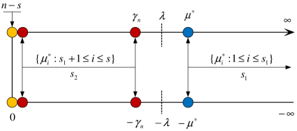
Figure 5: An illustration of three types of $\mu_{i}^{\star}$’s, that is, large $\boldsymbol{\mu}_{1}^{\star}$, bounded $\boldsymbol{\mu}_{2}^{\star}$ and zero $\boldsymbol{\mu}_{3}^{\star}$. The negative half of the real line is folded at 0 under the positive half for convenience. For the penalized least square method with a soft penalty function and under the assumption of fixed $d$, the specification of the regularization parameter $\lambda$ is that $\kappa_{n}\ll\lambda,~{}\alpha\gamma_{n}\leq\lambda,\text{ and }\lambda\ll\min\{\mu^{\star},\sqrt{n}\}$.

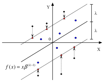
Figure 6: An illustration for the updating of responses with $d=1$. The solid black line is a fitted regression line. The dashed black lines are the corresponding shifted regression lines. The circle and diamond points are the original data points. The circle and triangle points are the updated data points. That is, the diamond points are drawn onto the shifted regression lines.

Lemma D.1.

A necessary and sufficient condition for $(\hat{\boldsymbol{\mu}},\hat{\boldsymbol{\beta}})$ to be a minimizer of $L(\boldsymbol{\mu},\boldsymbol{\beta})$ is that

$$\hat{\boldsymbol{\beta}}=(\boldsymbol{X}^{T}\boldsymbol{X})^{-1}\boldsymbol{X}^{T}(\boldsymbol{Y}-\hat{\boldsymbol{\mu}}),$$

$$Y_{i}-\hat{\mu}_{i}-\boldsymbol{X}_{i}^{T}\hat{\boldsymbol{\beta}}=\lambda\text{Sign}(\hat{\mu}_{i}),~{}~{}\text{ for }i\in\hat{I}_{0}^{c},$$

$$|Y_{i}-\boldsymbol{X}_{i}^{T}\hat{\boldsymbol{\beta}}|\leq\lambda,~{}~{}\text{ for }i\in\hat{I}_{0},$$

where $\text{Sign}(\cdot)$ is a sign function and $\hat{I}_{0}=\{1\leq i\leq n:\hat{\mu}_{i}=0\}$.

D.1 Proof of Lemma D.1

Proof of Lemma D.1.

By subdifferential calculus (see, for example, Theorem 3.27 in Jahn (2007)), a necessary and sufficient condition for $(\hat{\boldsymbol{\mu}},\hat{\boldsymbol{\beta}})$ to be a minimizer of $L(\boldsymbol{\mu},\boldsymbol{\beta})$ is that zero is in the subdifferential of $L$ at $(\hat{\boldsymbol{\mu}},\hat{\boldsymbol{\beta}})$, which means that, for each $i$,

$$\hat{\boldsymbol{\beta}}=(\boldsymbol{X}^{T}\boldsymbol{X})^{-1}\boldsymbol{X}^{T}(\boldsymbol{Y}-\hat{\boldsymbol{\mu}}),$$

$$Y_{i}-\hat{\mu}_{i}-\boldsymbol{X}_{i}^{T}\hat{\boldsymbol{\beta}}=\lambda\text{Sign}(\hat{\mu}_{i}),~{}~{}\text{ if }\hat{\mu}_{i}\not=0,$$

$$|Y_{i}-\boldsymbol{X}_{i}^{T}\hat{\boldsymbol{\beta}}|\leq\lambda,~{}~{}\text{ if }\hat{\mu}_{i}=0.$$

Thus, the conclusion of Lemma D.1 follows. ∎

Proposition D.2.

Suppose Assumptions (A) and (B) hold and there exist positive constants $C_{1}$ and $C_{2}$ such that $\lVert\boldsymbol{\beta}^{\star}\rVert_{2}<C_{1}$ and $\lVert\boldsymbol{\beta}^{(0)}\rVert_{2}<C_{2}$ wpg1. If $s_{1}\lambda/n=O(1)$ and $s_{2}\gamma_{n}/n=o(1)$, then, for every $K\geq 1$ and $k\leq K$, wpg1 as $n\rightarrow\infty$,

$$\lVert\boldsymbol{\beta}^{(K+1)}-\boldsymbol{\beta}^{(K)}\rVert_{2}\leq O((s_{1}/n)^{K}),\quad\mbox{and}\quad\lVert\boldsymbol{\beta}^{(k)}\rVert_{2}\leq 2\sqrt{d}C_{1}+C_{2}.$$

Remark 2.

For any prespecified critical value in the stopping rule, Proposition D.2 implies that the algorithm stops at the second iteration wpg1. In practice, the sample size $n$ might not be large enough for the two-iteration estimator to have a decent performance so that more iterations are usually needed to activate the stopping rule. By Proposition D.2, $K$ iterations will make the distance $\lVert\boldsymbol{\beta}^{(K+1)}-\boldsymbol{\beta}^{(K)}\rVert_{2}$ of the small order $(s_{1}/n)^{K}$. When $s_{1}/n$ is small, the algorithm converges quickly, which has been verified by our simulations.

D.2 Proof of Proposition D.2

Proof of Proposition D.2.

First, we show that, wpg1, $\lVert\boldsymbol{\beta}^{(1)}\rVert_{2}$ is bounded by $2\sqrt{d}C_{1}+C_{2}$. For each $k\geq 1$, we have

$$\mathbb{S}\boldsymbol{\beta}^{(k)} =\mathbb{S}_{S_{11}}^{\mu}+\mathbb{S}_{S_{12}}^{\mu}+\mathbb{S}_{S_{1}}\boldsymbol{\beta}^{\star}+\mathbb{S}_{S_{1}}^{\epsilon}+\mathbb{S}_{S_{2}\cup S_{3}}\boldsymbol{\beta}^{(k-1)}+\lambda(\mathcal{S}_{S_{2}}-\mathcal{S}_{S_{3}}),$$

where $S_{i}=\cup_{j=1}^{3}S_{ij}(\boldsymbol{\beta}^{(k-1)})$ for $i=1,2,3$ and $S_{ij}$’s are defined at the end of Section 2. Denote $\mathcal{A}_{k-1}$ as the event

$$\{S_{11}(\boldsymbol{\beta}^{(k-1)})=\emptyset,S_{12}(\boldsymbol{\beta}^{(k-1)})=S_{12}^{\star},S_{1}(\boldsymbol{\beta}^{(k-1)})=S_{10}^{\star}\cup S_{12}^{\star};S_{2}(\boldsymbol{\beta}^{(k-1)})=S_{21}^{\star};S_{3}(\boldsymbol{\beta}^{(k-1)})=S_{31}^{\star}\},$$

where $S_{ij}^{\star}$’s are defined at the beginning of Section 3.

By Lemma 3.1, $P(\mathcal{A}_{0})\rightarrow 1$. Thus, wpg1,

$$\boldsymbol{\beta}^{(1)}=T_{0}^{-1}T_{1}+T_{0}^{-1}T_{2}+T_{0}^{-1}T_{3}+T_{0}^{-1}T_{4}(\boldsymbol{\beta}^{(0)})+T_{0}^{-1}T_{5},$$

where $T_{0}=\mathbb{S}/n$, $T_{1}=\mathbb{S}_{S_{12}^{\star}}^{\mu}/n$, $T_{2}=\mathbb{S}_{s_{1}+1,n}\boldsymbol{\beta}^{\star}/n$, $T_{3}=\mathbb{S}_{s_{1}+1,n}^{\epsilon}/n$, $T_{4}(\boldsymbol{\beta}^{(0)})=\mathbb{S}_{1,s_{1}}\boldsymbol{\beta}^{(0)}/n$ and $T_{5}=(\mathbb{S}_{S_{21}^{\star}}-\mathbb{S}_{S_{31}^{\star}})\lambda/n$. We will show that, wpg1, $\lVert T_{0}^{-1}T_{1}\rVert_{2}\leq C_{2}/4$, $\lVert T_{0}^{-1}T_{2}\rVert_{2}\leq 2\sqrt{d}C_{1}$, $\lVert T_{0}^{-1}T_{3}\rVert_{2}\leq C_{2}/4$, $\lVert T_{0}^{-1}T_{4}(\boldsymbol{\beta}^{(0)})\rVert_{2}\leq C_{2}/4$ and $\lVert T_{0}^{-1}T_{5}\rVert_{2}\leq C_{2}/4$. Then, wpg1,

$$\lVert\boldsymbol{\beta}^{(1)}\rVert_{2}\leq\sum_{i=1}^{5}\lVert T_{0}^{-1}T_{i}\rVert_{2}\leq 2\sqrt{d}C_{1}+C_{2}.$$

On $T_{0}^{-1}T_{1}$. For $s_{2}\gamma_{n}/n=o(1)$, wpg1,

$$\lVert T_{0}^{-1}T_{1}\rVert_{2} \leq\lVert(\frac{1}{n}\mathbb{S})^{-1}\rVert_{F}\lVert\frac{1}{n}\mathbb{S}_{S_{12}^{\star}}^{\mu}\rVert_{2}\leq 4\lVert\boldsymbol{\Sigma}_{X}^{-1}\rVert_{F}\mathbb{E}\lVert\boldsymbol{X}_{0}\rVert_{2}\frac{s_{2}}{n}\gamma_{n}\rightarrow 0.$$

Thus, wpg1, $\lVert T_{0}^{-1}T_{1}\rVert_{2}\leq C_{2}/4$.

On $T_{0}^{-1}T_{2}$. Wpg1,

$$\lVert T_{0}^{-1}T_{2}\rVert_{2} \leq\lVert(\frac{1}{n}\mathbb{S})^{-1}\frac{1}{n}\mathbb{S}_{s_{1}+1,n}\rVert_{F}\lVert\boldsymbol{\beta}^{\star}\rVert_{2}\leq 2\lVert\boldsymbol{I}_{d}\rVert_{F}C_{1}=2\sqrt{d}C_{1}.$$

On $T_{0}^{-1}T_{3}$. Wpg1,

$$\lVert T_{0}^{-1}T_{3}\rVert_{2} \leq 2\lVert\boldsymbol{\Sigma}_{X}^{-1}\rVert_{F}\lVert\frac{1}{n}\mathbb{S}_{s_{1}+1,n}^{\epsilon}\rVert_{2}\overset{P}{\longrightarrow}0.$$

Thus, wpg1, $\lVert T_{0}^{-1}T_{3}\rVert_{2}\leq C_{2}/4$.

On $T_{0}^{-1}T_{4}(\boldsymbol{\beta}^{(0)})$. For $s_{1}/n=o(1)$,

$$\lVert T_{0}^{-1}T_{4}(\boldsymbol{\beta}^{(0)})\rVert_{2} \leq\frac{s_{1}}{n}\lVert(\frac{1}{n}\mathbb{S})^{-1}\frac{1}{s_{1}}\mathbb{S}_{1,s_{1}}\rVert_{F}\lVert\boldsymbol{\beta}^{(0)}\rVert_{2}\leq\frac{s_{1}}{n}2\sqrt{d}C_{2}\overset{P}{\longrightarrow}0.$$

Thus, wpg1, $\lVert T_{0}^{-1}T_{4}(\boldsymbol{\beta}^{(0)})\rVert_{2}\leq C_{2}/4$.

On $T_{0}^{-1}T_{5}$. For $s_{1}\lambda/n=O(1)$, wpg1,

$$\lVert T_{0}^{-1}T_{5}\rVert_{2} \leq 2\lVert\boldsymbol{\Sigma}_{X}^{-1}\rVert_{F}\frac{s_{1}\lambda}{n}(\lVert\frac{1}{s_{1}}\mathcal{S}_{S_{21}^{\star}}\rVert_{2}+\lVert\frac{1}{s_{1}}\mathcal{S}_{S_{31}^{\star}}\rVert_{2})\overset{P}{\longrightarrow}0.$$

Thus, wpg1, $\lVert T_{0}^{-1}T_{5}\rVert_{2}\leq C_{2}/4$.

Next, consider $\lVert\boldsymbol{\beta}_{2}-\boldsymbol{\beta}_{1}\rVert_{2}$. Since $\boldsymbol{\beta}^{(1)}$ is bounded wpg1, by Lemma 3.1, $\mathcal{A}_{1}$ occurs wpg1. Then,

$$\boldsymbol{\beta}^{(2)}=T_{0}^{-1}T_{1}+T_{0}^{-1}T_{2}+T_{0}^{-1}T_{3}+T_{0}^{-1}T_{4}(\boldsymbol{\beta}^{(1)})+T_{0}^{-1}T_{5},$$

where $T_{4}(\boldsymbol{\beta}^{(1)})=(1/n)\mathbb{S}_{1,s_{1}}\boldsymbol{\beta}^{(1)}.$ Thus, wpg1,

$$\boldsymbol{\beta}^{(2)}-\boldsymbol{\beta}^{(1)}=\mathbb{S}^{-1}\mathbb{S}_{1,s_{1}}(\boldsymbol{\beta}^{(1)}-\boldsymbol{\beta}^{(0)}).$$

It follows that, for $s_{1}=o(n)$, wpg1,

$$\lVert\boldsymbol{\beta}^{(2)}-\boldsymbol{\beta}^{(1)}\rVert_{2}\leq\lVert\mathbb{S}^{-1}\mathbb{S}_{1,s_{1}}\rVert_{F}\lVert\boldsymbol{\beta}^{(1)}-\boldsymbol{\beta}^{(0)}\rVert_{2}\leq(2\sqrt{d}s_{1}/n)(4\sqrt{d}C_{1}+2C_{2})\rightarrow 0.$$

Then, wpg1, $\boldsymbol{\beta}^{(2)}=\boldsymbol{\beta}^{(1)}$, which means that, wpg1, the iteration algorithm stops at the second iteration.

Finally, for any $K\geq 1$, repeat the above arguments. Then, with at least probability $p_{n,K}=P(\bigcap_{k=0}^{K}\mathcal{A}_{k})$, which increases to one by Lemma 3.1, we have

$$\lVert\boldsymbol{\beta}^{(K+1)}-\boldsymbol{\beta}^{(K)}\rVert_{2}\leq(2\sqrt{d}s_{1}/n)^{K}(4\sqrt{d}C_{1}+2C_{2})=O((s_{1}/n)^{K})\rightarrow 0,$$

and $\lVert\boldsymbol{\beta}^{(k)}\rVert_{2}\leq 2\sqrt{d}C_{1}+C_{2}$ for all $k\leq K$. ∎

Long Proof of Lemma D.2.

First, we show that, wpg1, $\lVert\boldsymbol{\beta}^{(1)}\rVert_{2}$ is bounded by $2\sqrt{d}C_{1}+C_{2}$. For each $k\geq 1$, we have

$$\mathbb{S}\boldsymbol{\beta}^{(k)} =\sum_{i\in S_{1}}\boldsymbol{X}_{i}Y_{i}+\sum_{i\in S_{2}}\boldsymbol{X}_{i}(\boldsymbol{X}_{i}^{T}\boldsymbol{\beta}^{(k-1)}+\lambda)+\sum_{i\in S_{3}}\boldsymbol{X}_{i}(\boldsymbol{X}_{i}^{T}\boldsymbol{\beta}^{(k-1)}-\lambda)$$

$$=\sum_{i\in S_{1}}\boldsymbol{X}_{i}(\mu_{i}^{\star}+\boldsymbol{X}_{i}^{T}\boldsymbol{\beta}^{\star}+\epsilon_{i})+\sum_{i\in S_{2}}\boldsymbol{X}_{i}(\boldsymbol{X}_{i}^{T}\boldsymbol{\beta}^{(k-1)}+\lambda)+\sum_{i\in S_{3}}\boldsymbol{X}_{i}(\boldsymbol{X}_{i}^{T}\boldsymbol{\beta}^{(k-1)}-\lambda)$$

$$=\sum_{i\in S_{1}}\boldsymbol{X}_{i}\mu_{i}^{\star}+\sum_{i\in S_{1}}\boldsymbol{X}_{i}\boldsymbol{X}_{i}^{T}\boldsymbol{\beta}^{\star}+\sum_{i\in S_{1}}\boldsymbol{X}_{i}\epsilon_{i}+\sum_{i\in S_{2}\cup S_{3}}\boldsymbol{X}_{i}\boldsymbol{X}_{i}^{T}\boldsymbol{\beta}^{(k-1)}+\lambda(\sum_{i\in S_{2}}\boldsymbol{X}_{i}-\sum_{i\in S_{3}}\boldsymbol{X}_{i})$$

$$=\sum_{i\in S_{11}}\boldsymbol{X}_{i}\mu_{i}^{\star}+\sum_{i\in S_{12}}\boldsymbol{X}_{i}\mu_{i}^{\star}+\sum_{i\in S_{1}}\boldsymbol{X}_{i}\boldsymbol{X}_{i}^{T}\boldsymbol{\beta}^{\star}+\sum_{i\in S_{1}}\boldsymbol{X}_{i}\epsilon_{i}+\sum_{i\in S_{2}\cup S_{3}}\boldsymbol{X}_{i}\boldsymbol{X}_{i}^{T}\boldsymbol{\beta}^{(k-1)}+\lambda(\sum_{i\in S_{2}}\boldsymbol{X}_{i}-\sum_{i\in S_{3}}\boldsymbol{X}_{i}),$$

where the index sets all depend on $\boldsymbol{\beta}^{(k-1)}$. Specifically,

$$S_{1}=S_{1}(\boldsymbol{\beta}^{(k-1)}) =\{1\leq i\leq n:|Y_{i}-\boldsymbol{X}_{i}^{T}\boldsymbol{\beta}^{(k-1)}|\leq\lambda\},$$

$$S_{2}=S_{2}(\boldsymbol{\beta}^{(k-1)}) =\{1\leq i\leq n:Y_{i}-\boldsymbol{X}_{i}^{T}\boldsymbol{\beta}^{(k-1)}>\lambda\},$$

$$S_{3}=S_{3}(\boldsymbol{\beta}^{(k-1)}) =\{1\leq i\leq n:Y_{i}-\boldsymbol{X}_{i}^{T}\boldsymbol{\beta}^{(k-1)}<-\lambda\},$$

$$S_{11}=S_{11}(\boldsymbol{\beta}^{(k-1)}) =\{1\leq i\leq s_{1}:|Y_{i}-\boldsymbol{X}_{i}^{T}\boldsymbol{\beta}^{(k-1)}|\leq\lambda\},$$

$$S_{12}=S_{11}(\boldsymbol{\beta}^{(k-1)}) =\{s_{1}+1\leq i\leq s:|Y_{i}-\boldsymbol{X}_{i}^{T}\boldsymbol{\beta}^{(k-1)}|\leq\lambda\}.$$

Denote an event

$$\mathcal{A}_{k-1}=\{S_{11}(\boldsymbol{\beta}^{(k-1)})=\emptyset,S_{12}(\boldsymbol{\beta}^{(k-1)})=S_{12}^{\star},S_{1}(\boldsymbol{\beta}^{(k-1)})=S_{10}^{\star}\cup S_{12}^{\star};S_{2}(\boldsymbol{\beta}^{(k-1)})=S_{21}^{\star};S_{3}(\boldsymbol{\beta}^{(k-1)})=S_{31}^{\star}\}.$$

By Lemma 3.1, $P(\mathcal{A}_{0})\rightarrow 1$.

Thus, wpg1, we have

$$\boldsymbol{\beta}^{(1)}=T_{0}^{-1}T_{1}+T_{0}^{-1}T_{2}+T_{0}^{-1}T_{3}+T_{0}^{-1}T_{4}(\boldsymbol{\beta}^{(0)})+T_{0}^{-1}T_{5},$$

where

$$T_{0} =\frac{1}{n}\mathbb{S},$$

$$T_{1} =\frac{1}{n}\mathbb{S}_{S_{12}^{\star}}^{\mu},$$

$$T_{2} =\frac{1}{n}\mathbb{S}_{s_{1}+1,n}\boldsymbol{\beta}^{\star},$$

$$T_{3} =\frac{1}{n}\mathbb{S}_{s_{1}+1,n}^{\epsilon},$$

$$T_{4}(\boldsymbol{\beta}^{(0)}) =\frac{1}{n}\mathbb{S}_{1,s_{1}}\boldsymbol{\beta}^{(0)},$$

$$T_{5} =\frac{1}{n}(\mathbb{S}_{S_{21}^{\star}}-\mathbb{S}_{S_{31}^{\star}})\lambda.$$

We will show that, wpg1,

$$\lVert T_{0}^{-1}T_{1}\rVert_{2}\leq C_{2}/4,$$

$$\lVert T_{0}^{-1}T_{2}\rVert_{2}\leq 2\sqrt{d}C_{1},$$

$$\lVert T_{0}^{-1}T_{3}\rVert_{2}\leq C_{2}/4,$$

$$\lVert T_{0}^{-1}T_{4}(\boldsymbol{\beta}^{(0)})\rVert_{2}\leq C_{2}/4,$$

$$\lVert T_{0}^{-1}T_{5}\rVert_{2}\leq C_{2}/4.$$

Thus, we have, wpg1,

$$\lVert\boldsymbol{\beta}^{(1)}\rVert_{2}\leq\sum_{i=1}^{5}\lVert T_{0}^{-1}T_{i}\rVert_{2}\leq 2\sqrt{d}C_{1}+C_{2}.$$

On $T_{0}^{-1}T_{1}$. We have, for $s_{2}\gamma_{n}/n=o(1)$, wpg1,

$$\lVert T_{0}^{-1}T_{1}\rVert_{2} =\lVert(\frac{1}{n}\mathbb{S})^{-1}\frac{1}{n}\mathbb{S}_{S_{12}^{\star}}^{\mu}\rVert_{2}$$

$$\leq\lVert(\frac{1}{n}\mathbb{S})^{-1}\rVert_{F}\lVert\frac{1}{n}\mathbb{S}_{S_{12}^{\star}}^{\mu}\rVert_{2}$$

$$\leq\lVert(\frac{1}{n}\mathbb{S})^{-1}\rVert_{F}\lVert\frac{1}{n}\sum_{i=s_{1}+1}^{s}\boldsymbol{X}_{i}\mu_{i}\rVert_{2}$$

$$=\lVert(\frac{1}{n}\mathbb{S})^{-1}\rVert_{F}\frac{s_{2}}{n}\lVert\frac{1}{s_{2}}\sum_{i=s_{1}+1}^{s}\boldsymbol{X}_{i}\mu_{i}\rVert_{2}$$

$$\leq\lVert(\frac{1}{n}\mathbb{S})^{-1}\rVert_{F}\frac{s_{2}}{n}\gamma_{n}\frac{1}{s_{2}}\sum_{i=s_{1}+1}^{s}\lVert\boldsymbol{X}_{i}\rVert_{2}$$

$$(wpg1) \leq 2\lVert\boldsymbol{\Sigma}_{X}^{-1}\rVert_{F}\frac{s_{2}}{n}\gamma_{n}2\mathbb{E}\lVert\boldsymbol{X}_{0}\rVert_{2}$$

$$=4\lVert\boldsymbol{\Sigma}_{X}^{-1}\rVert_{F}\mathbb{E}\lVert\boldsymbol{X}_{0}\rVert_{2}\frac{s_{2}}{n}\gamma_{n}\rightarrow 0.$$

Thus, we have, wpg1, $\lVert T_{0}^{-1}T_{1}\rVert_{2}\leq C_{2}/4$.

On $T_{0}^{-1}T_{2}$. We have, wpg1,

$$\lVert T_{0}^{-1}T_{2}\rVert_{2} =\lVert(\frac{1}{n}\mathbb{S})^{-1}\frac{1}{n}\mathbb{S}_{s_{1}+1,n}\boldsymbol{\beta}^{\star}\rVert_{2}$$

$$\leq\lVert(\frac{1}{n}\mathbb{S})^{-1}\frac{1}{n}\mathbb{S}_{s_{1}+1,n}\rVert_{F}\lVert\boldsymbol{\beta}^{\star}\rVert_{2}$$

$$\leq\lVert(\frac{1}{n}\mathbb{S})^{-1}\frac{1}{n}\mathbb{S}_{s_{1}+1,n}\rVert_{F}C_{1}$$

$$(wpg1) \leq 2\lVert\boldsymbol{\Sigma}_{X}^{-1}\boldsymbol{\Sigma}_{X}\rVert_{F}C_{1}$$

$$=2\lVert\boldsymbol{I}_{d}\rVert_{F}C_{1}$$

$$=2\sqrt{d}C_{1}.$$

On $T_{0}^{-1}T_{3}$. We have, wpg1,

$$\lVert T_{0}^{-1}T_{3}\rVert_{2} =\lVert(\frac{1}{n}\mathbb{S})^{-1}\frac{1}{n}\mathbb{S}_{s_{1}+1,n}^{\epsilon}\rVert_{2}$$

$$=\lVert(\frac{1}{n}\mathbb{S})^{-1}\rVert_{F}\lVert\frac{1}{n}\mathbb{S}_{s_{1}+1,n}^{\epsilon}\rVert_{2}$$

$$(wpg1) \leq 2\lVert\boldsymbol{\Sigma}_{X}^{-1}\rVert_{F}\lVert\frac{1}{n}\mathbb{S}_{s_{1}+1,n}^{\epsilon}\rVert_{2}\overset{P}{\longrightarrow}0.$$

Thus, wpg1, $\lVert T_{0}^{-1}T_{3}\rVert_{2}\leq C_{2}/4$.

On $T_{0}^{-1}T_{4}(\boldsymbol{\beta}^{(0)})$. We have,

$$\lVert T_{0}^{-1}T_{4}(\boldsymbol{\beta}^{(0)})\rVert_{2} =\lVert(\frac{1}{n}\mathbb{S})^{-1}\frac{1}{n}\mathbb{S}_{1,s_{1}}\boldsymbol{\beta}^{(0)}\rVert_{2}$$

$$\leq\lVert(\frac{1}{n}\mathbb{S})^{-1}\rVert_{F}\lVert\frac{1}{n}\mathbb{S}_{1,s_{1}}\boldsymbol{\beta}^{(0)}\rVert_{2}$$

$$\leq\lVert(\frac{1}{n}\mathbb{S})^{-1}\rVert_{F}\lVert\frac{1}{n}\mathbb{S}_{1,s_{1}}\rVert_{2}\lVert\boldsymbol{\beta}^{(0)}\rVert_{2}$$

$$(wpg1) \leq 2\lVert\boldsymbol{\Sigma}_{X}^{-1}\rVert_{F}\lVert\frac{1}{n}\mathbb{S}_{1,s_{1}}\rVert_{2}C_{2}\overset{P}{\longrightarrow}0.$$

Thus, wpg1, $\lVert T_{0}^{-1}T_{4}(\boldsymbol{\beta}^{(0)})\rVert_{2}\leq C_{2}/4$.

On $T_{0}^{-1}T_{5}$. For $s_{1}\lambda/n=O(1)$, wpg1,

$$\lVert T_{0}^{-1}T_{5}\rVert_{2} =\lVert(\frac{1}{n}\mathbb{S})^{-1}\frac{1}{n}(\mathcal{S}_{S_{21}^{\star}}-\mathcal{S}_{S_{31}^{\star}})\lambda\rVert_{2}$$

$$\leq\lVert(\frac{1}{n}\mathbb{S})^{-1}\rVert_{F}\frac{s_{1}\lambda}{n}(\lVert\frac{1}{s_{1}}\mathcal{S}_{S_{21}^{\star}}-\frac{1}{s_{1}}\mathcal{S}_{S_{31}^{\star}}\rVert_{2})$$

$$\leq\lVert(\frac{1}{n}\mathbb{S})^{-1}\rVert_{F}\frac{s_{1}\lambda}{n}(\lVert\frac{1}{s_{1}}\mathcal{S}_{S_{21}^{\star}}\rVert_{2}+\lVert\frac{1}{s_{1}}\mathcal{S}_{S_{31}^{\star}}\rVert_{2})$$

$$(wpg1) \leq 2\lVert\boldsymbol{\Sigma}_{X}^{-1}\rVert_{F}\frac{s_{1}\lambda}{n}(\lVert\frac{1}{s_{1}}\mathcal{S}_{S_{21}^{\star}}\rVert_{2}+\lVert\frac{1}{s_{1}}\mathcal{S}_{S_{31}^{\star}}\rVert_{2})\overset{P}{\longrightarrow}0.$$

Thus, wpg1, $\lVert T_{0}^{-1}T_{5}\rVert_{2}\leq C_{2}/4$.

Next, consider $\lVert\boldsymbol{\beta}_{2}-\boldsymbol{\beta}_{1}\rVert_{2}$. Since $\boldsymbol{\beta}^{(1)}$ is bounded wpg1, by Lemma 3.1, $\mathcal{A}_{1}$ occurs wpg1.

Then,

$$\boldsymbol{\beta}^{(2)}=T_{0}^{-1}T_{1}+T_{0}^{-1}T_{2}+T_{0}^{-1}T_{3}+T_{0}^{-1}T_{4}(\boldsymbol{\beta}^{(1)})+T_{0}^{-1}T_{5},$$

where

$$T_{4}(\boldsymbol{\beta}^{(1)}) =\frac{1}{n}\mathbb{S}_{1,s_{1}}\boldsymbol{\beta}^{(1)}.$$

Thus, wpg1,

$$\boldsymbol{\beta}^{(2)}-\boldsymbol{\beta}^{(1)}=\mathbb{S}^{-1}\mathbb{S}_{1,s_{1}}(\boldsymbol{\beta}^{(1)}-\boldsymbol{\beta}^{(0)}).$$

Thus, for $s_{1}=o(n)$,

$$\lVert\boldsymbol{\beta}^{(2)}-\boldsymbol{\beta}^{(1)}\rVert_{2}\leq\lVert\mathbb{S}^{-1}\mathbb{S}_{1,s_{1}}\rVert_{F}\lVert\boldsymbol{\beta}^{(1)}-\boldsymbol{\beta}^{(0)}\rVert_{2}\leq(2\sqrt{d}s_{1}/n)(4\sqrt{d}C_{1}+2C_{2})\rightarrow 0.$$

Thus, wpg1, $\boldsymbol{\beta}^{(2)}=\boldsymbol{\beta}^{(1)}$, which means that, wpg1, the iteration algorithm converges at the first iteration.

For any $K\geq 1$, Repeat the above arguments, with at least probability $p_{n,K}=P(\bigcap_{k=0}^{K}\mathcal{A}_{k})$, we have

$$\lVert\boldsymbol{\beta}^{(K+1)}-\boldsymbol{\beta}^{(K)}\rVert_{2}\leq(2\sqrt{d}s_{1}/n)^{K}(4\sqrt{d}C_{1}+2C_{2})=O((s_{1}/n)^{K})\rightarrow 0,$$

and $\lVert\boldsymbol{\beta}^{(K+1)}-\boldsymbol{\beta}^{(K)}\rVert_{2}\leq O((s_{1}/n)^{K})$. ∎

Lemma D.3.

A necessary and sufficient condition for $(\hat{\boldsymbol{\mu}},\hat{\boldsymbol{\beta}})$ to be a minimizer of $L(\boldsymbol{\mu},\boldsymbol{\beta})$ is that it is a solution to equations (2.5) and (2.6).

D.3 Proof of Lemma D.3

Proof of Lemma D.3.

First, we show a solution of (2.5) and (2.6) satisfies the necessary and sufficient condition in Lemma D.1. Denote a solution of (2.5) and (2.6) as $(\hat{\boldsymbol{\mu}},\hat{\boldsymbol{\beta}})$. Then $\hat{\boldsymbol{\beta}}=(\boldsymbol{X}^{T}\boldsymbol{X})^{-1}\boldsymbol{X}^{T}(\boldsymbol{Y}-\hat{\boldsymbol{\mu}})$, which is exactly the first condition in Lemma D.1, and, for each $i=1,2,\cdots,n$, $(\hat{\boldsymbol{\mu}},\hat{\boldsymbol{\beta}})$ satisfies one of three cases: $|Y_{i}-\boldsymbol{X}_{i}^{T}\hat{\boldsymbol{\beta}}|\leq\lambda$ and $\hat{\mu}_{i}=0$; $Y_{i}-\boldsymbol{X}_{i}^{T}\hat{\boldsymbol{\beta}}>\lambda$ and $\hat{\mu}_{i}=Y_{i}-\boldsymbol{X}_{i}^{T}\hat{\boldsymbol{\beta}}-\lambda$; $Y_{i}-\boldsymbol{X}_{i}^{T}\hat{\boldsymbol{\beta}}<-\lambda$ and $\hat{\mu}_{i}=Y_{i}-\boldsymbol{X}_{i}^{T}\hat{\boldsymbol{\beta}}+\lambda$. If $(\hat{\boldsymbol{\mu}},\hat{\boldsymbol{\beta}})$ satisfies the first case, it satisfies the third condition in Lemma D.1. If $(\hat{\boldsymbol{\mu}},\hat{\boldsymbol{\beta}})$ satisfies the second case, then $\hat{\mu}_{i}>0$ and $Y_{i}-\hat{\mu}_{i}-\boldsymbol{X}_{i}^{T}\hat{\boldsymbol{\beta}}=\lambda=\lambda\text{Sign}(\hat{\mu}_{i})$, which means that the second case satisfies the second condition in Lemma D.1. Similarly, the third case also satisfies the second condition in Lemma D.1. Thus $(\hat{\boldsymbol{\mu}},\hat{\boldsymbol{\beta}})$ satisfies the necessary and sufficient condition in Lemma D.1.

In the other direction, suppose $(\hat{\boldsymbol{\mu}},\hat{\boldsymbol{\beta}})$ satisfies the necessary and sufficient condition in Lemma D.1. Then, the first condition in Lemma D.1 exactly $(\ref{eq2.4})$. For each $i$, $(\hat{\boldsymbol{\mu}},\hat{\boldsymbol{\beta}})$ satisfies one of three cases: $\hat{\mu}_{i}=0$ and $|Y_{i}-\boldsymbol{X}_{i}^{T}\hat{\boldsymbol{\beta}}|\leq\lambda$; $\hat{\mu}_{i}>0$ and $Y_{i}-\hat{\mu}_{i}-\boldsymbol{X}_{i}^{T}\hat{\boldsymbol{\beta}}=\lambda$; $\hat{\mu}_{i}<0$ and $Y_{i}-\hat{\mu}_{i}-\boldsymbol{X}_{i}^{T}\hat{\boldsymbol{\beta}}=-\lambda$. If $(\hat{\boldsymbol{\mu}},\hat{\boldsymbol{\beta}})$ satisfies the first case, it satisfies the first case in (2.6). If $(\hat{\boldsymbol{\mu}},\hat{\boldsymbol{\beta}})$ satisfies the second case, then $\hat{\mu}_{i}=Y_{i}-\boldsymbol{X}_{i}^{T}\hat{\boldsymbol{\beta}}-\lambda$ and $Y_{i}-\boldsymbol{X}_{i}^{T}\hat{\boldsymbol{\beta}}>\lambda$, which means that $(\hat{\boldsymbol{\mu}},\hat{\boldsymbol{\beta}})$ satisfies the second case of (2.6). Similarly, If $(\hat{\boldsymbol{\mu}},\hat{\boldsymbol{\beta}})$ satisfies the third case, then it satisfies the third case of (2.6). Thus, $(\hat{\boldsymbol{\mu}},\hat{\boldsymbol{\beta}})$ satisfies (2.5) and (2.6). ∎

Appendix E Supplement for Section 3

In this supplement, we provide the proofs of the theoretical results in Section 3. Before that, we point out that those two different sufficient conditions in Theorem 3.2 come from the different analysis on the term $\mathbb{S}_{S_{12}^{\star}}^{\mu}$. Each of the two different sufficient conditions does not imply the other. Specifically, on one hand, suppose the absolute values of $\mu_{i}^{\star}$’s are all equal for $i=s_{1}+1,s_{2}+2,\cdots,s$. Then, $\lVert\boldsymbol{\mu}_{2}^{\star}\rVert_{2}^{2+\delta}=s_{2}^{(2+\delta)/2}|\mu_{s}^{\star}|^{2+\delta}$ and $\sum_{i=s_{1}+1}^{s}|\mu^{\star}_{i}|^{2+\delta}=s_{2}|\mu_{s}^{\star}|^{2+\delta}$. Thus Assumption (C) holds automatically since $s_{2}\rightarrow\infty$. This means that Assumption (C) holds at least when the absolute magnitudes of $\mu_{i}^{\star}$’s are similar to each other. For this case, there still exists a consistent estimator even if $n/(\kappa_{n}\gamma_{n})\ll s_{2}\ll n$. On the other hand, suppose $\mu_{s}^{\star}=\gamma_{n}$ and the other $\mu_{i}^{\star}$’s are all equal to a constant $c>0$. Then, $\lVert\boldsymbol{\mu}_{2}^{\star}\rVert_{2}^{2+\delta}=[\gamma_{n}^{2}+(s_{2}-1)c^{2}]^{(2+\delta)/2}$ and $\sum_{i=s_{1}+1}^{s}|\mu^{\star}_{i}|^{2+\delta}=\gamma_{n}^{2+\delta}+(s_{2}-1)c^{2+\delta}$. If $s_{2}\ll\gamma_{n}^{2}\ll n/(\kappa_{n}\gamma_{n})$, the previous two terms are both asymptotically equivalent to $\gamma_{n}^{2+\delta}$. Thus Assumption (C) fails but the other sufficient condition holds.

E.1 Proof of Lemma 3.1

Proof of Lemma 3.1.

The proof is the similar to that of Lemma 4.1 and omitted. ∎

E.2 Proof of Theorems 3.2

Proof of Theorems 3.2.

By Lemma 3.1, wpg1, the solution $\hat{\boldsymbol{\beta}}_{n}$ to $\varphi_{n}(\boldsymbol{\beta})=0$ on $\mathcal{B}_{C}(\boldsymbol{\beta}^{\star})$ is explicitly given by

$$\hat{\boldsymbol{\beta}}_{n}=\boldsymbol{\beta}^{\star}+T_{0}^{-1}(T_{1}+T_{2}+T_{3}-T_{4}),$$

where $T_{0}=(1/n)\mathbb{S}_{s_{1}+1,n}$, $T_{1}=(1/n)\mathbb{S}_{S_{12}^{\star}}^{\mu}$, $T_{2}=(1/n)\mathbb{S}_{s_{1}+1,n}^{\epsilon}$, $T_{3}=(\lambda/n)\mathcal{S}_{S_{21}^{\star}}$ and $T_{4}=(\lambda/n)\mathcal{S}_{S_{31}^{\star}}$. We will show that $T_{0}\overset{P}{\longrightarrow}\boldsymbol{\boldsymbol{\Sigma}}_{X}^{-1}>0$ with the Frobenius norm and $T_{i}\overset{P}{\longrightarrow}0$ with the Euclidean norm for $i=1,2,3,4$. Thus, by Slutsky’s lemma (see, for example, Lemma 2.8 on page 11 of van der Vaart (1998)), $\hat{\boldsymbol{\beta}}_{n}$ is a consistent estimator of $\boldsymbol{\beta}^{\star}$.

On $T_{0}^{-1}$. By law of large number, $T_{0}\overset{P}{\longrightarrow}\boldsymbol{\boldsymbol{\Sigma}}_{X}>0$. Then, by continuous mapping theorem, $T_{0}^{-1}\overset{P}{\longrightarrow}\boldsymbol{\boldsymbol{\Sigma}}_{X}^{-1}>0$.

On $T_{1}$: Approach One. Suppose $s_{2}=o(n/(\kappa_{n}\gamma_{n}))$. Then,

$$\lVert T_{1}\rVert_{2} \leq\frac{1}{n}\sum_{i=s_{1}+1}^{s}\lVert\boldsymbol{X}_{i}\mu_{i}^{\star}\rVert_{2}=\frac{1}{n}\sum_{i=s_{1}+1}^{s}\lVert\boldsymbol{X}_{i}\rVert_{2}\cdot|\mu_{i}^{\star}|\leq s_{2}\kappa_{n}\gamma_{n}/n=o(1).$$

On $T_{1}$: Approach Two. Under Assumption (C), it follows $(\boldsymbol{\boldsymbol{\Sigma}}_{X}\sum_{i=s_{1}+1}^{s}\mu^{\star 2}_{i})^{-1/2}\mathbb{S}_{S_{12}^{\star}}^{\mu}\overset{d}{\longrightarrow}N(0,I_{d})$. In fact, Assumption (C) implies the Lyapunov condition for sequence of random vectors (see, e.g. Proposition 2.27 on page 332 of (van der Vaart, 1998)). More specifically, recall the Lyapunov condition is that there exists some constant $\delta>0$ such that

$$\sum_{i=s_{1}+1}^{s}\mathbb{E}\lVert(\boldsymbol{\boldsymbol{\Sigma}}_{X}\sum_{j=s_{1}+1}^{s}\mu^{\star 2}_{j})^{-1/2}\boldsymbol{X}_{i}\mu_{i}^{\star}\rVert_{2}^{2+\delta}\rightarrow 0.$$

Then, by Assumption (C),

$$\sum_{i=s_{1}+1}^{s}\mathbb{E}\lVert(\boldsymbol{\boldsymbol{\Sigma}}_{X}\sum_{j=s_{1}+1}^{s}\mu^{\star 2}_{j})^{-\frac{1}{2}}\boldsymbol{X}_{i}\mu_{i}^{\star}\rVert_{2}^{2+\delta}\leq(\sum_{j=s_{1}+1}^{s}\mu^{\star 2}_{j})^{-\frac{2+\delta}{2}}\sum_{i=s_{1}+1}^{s}|\mu_{i}^{\star}|^{2+\delta}\lambda_{\min}^{-\frac{2+\delta}{2}}\mathbb{E}\lVert X_{0}\rVert_{2}^{2+\delta}\longrightarrow 0,$$

where $\lambda_{\min}>0$ is the minimum eigenvalue of $\boldsymbol{\boldsymbol{\Sigma}}_{X}$. Then,

$$\lVert T_{1}\rVert_{2} =\lVert\frac{1}{n}\mathbb{S}_{S_{12}^{\star}}^{\mu}\rVert_{2}\leq\frac{1}{n}\lVert(\boldsymbol{\boldsymbol{\Sigma}}_{X}\sum_{i=s_{1}+1}^{s}\mu^{\star 2}_{i})^{1/2}\rVert_{F}\lVert(\boldsymbol{\boldsymbol{\Sigma}}_{X}\sum_{i=s_{1}+1}^{s}\mu^{\star 2}_{i})^{-1/2}\mathbb{S}_{S_{12}^{\star}}^{\mu}\rVert_{2}$$

$$=\frac{1}{n}(\sum_{i=s_{1}+1}^{s}\mu^{\star 2}_{i})^{1/2}\lVert\boldsymbol{\boldsymbol{\Sigma}}_{X}^{1/2}\rVert_{F}O_{P}(1)\leq\frac{1}{n}(s_{2}\gamma_{n}^{2})^{1/2}O_{P}(1)\leq\frac{1}{\sqrt{n}}\gamma_{n}O_{P}(1)=o_{P}(1).$$

On $T_{2}$. By law of large number, $T_{2}=o_{P}(1)$.

On $T_{3}$ and $T_{4}$. By noting $\lambda\ll\sqrt{n}$,

$$\lVert T_{3}\rVert_{2}=\lVert\lambda\frac{1}{n}\mathcal{S}_{S_{21}^{\star}}\rVert_{2}=\lambda\frac{\sqrt{s_{1}}}{n}\lVert\frac{1}{\sqrt{s_{1}}}\mathcal{S}_{S_{21}^{\star}}\rVert_{2}\leq\frac{\lambda}{\sqrt{n}}O_{P}(1)=o_{P}(1).$$

Thus $T_{3}=o_{P}(1)$. In the same way, we can show that $T_{4}=o_{P}(1)$ holds. ∎

In Theorem, one condition is $D_{n}/n=o(1)$. It turns out we can consider other conditions on $D_{n}$ and derive more possible asymptotic distributions for $\hat{\boldsymbol{\beta}}_{n}$.

Theorem E.1 (Asymptotic Distributions on $\hat{\boldsymbol{\beta}}_{n}$: more cases).

Under Assumptions (A), (B) and (C), for all constants $b,c\in\mathbb{R}^{+}$,

1. when $s_{1}\ll n/\lambda^{2}$ and $D_{n}^{2}/n=o(1)$, $\sqrt{n}(\hat{\boldsymbol{\beta}}_{n}-\boldsymbol{\beta}^{\star})\overset{d}{\longrightarrow}N(0,\sigma^{2}\boldsymbol{\boldsymbol{\Sigma}}_{X}^{-1})$; [main case]

2. when $s_{1}\ll n/\lambda^{2}$ and $D_{n}^{2}/n\sim c$, $\sqrt{n}(\hat{\boldsymbol{\beta}}_{n}-\boldsymbol{\beta}^{\star})\overset{d}{\longrightarrow}N(0,(c+\sigma^{2})\boldsymbol{\boldsymbol{\Sigma}}_{X}^{-1});$

3. when $s_{1}\ll n/\lambda^{2}$ and $D_{n}^{2}/n\rightarrow\infty$, $r_{n}(\hat{\boldsymbol{\beta}}_{n}-\boldsymbol{\beta}^{\star})\overset{d}{\longrightarrow}N(0,\boldsymbol{\boldsymbol{\Sigma}}_{X}^{-1}),$ where $r_{n}\sim n/D_{n}\ll\sqrt{n}$;

4. when $s_{1}\sim bn/\lambda^{2}$ and $D_{n}^{2}/n=o(1)$, $\sqrt{n}(\hat{\boldsymbol{\beta}}_{n}-\boldsymbol{\beta}^{\star})\overset{d}{\longrightarrow}N(0,(b+\sigma^{2})\boldsymbol{\boldsymbol{\Sigma}}_{X}^{-1});$

5. when $s_{1}\sim bn/\lambda^{2}$ and $D_{n}^{2}/n\sim c$, $\sqrt{n}(\hat{\boldsymbol{\beta}}_{n}-\boldsymbol{\beta}^{\star})\overset{d}{\longrightarrow}N(0,(b+c+\sigma^{2})\boldsymbol{\boldsymbol{\Sigma}}_{X}^{-1});$

6. when $s_{1}\sim bn/\lambda^{2}$ and $D_{n}^{2}/n\rightarrow\infty$, $r_{n}(\hat{\boldsymbol{\beta}}_{n}-\boldsymbol{\beta}^{\star})\overset{d}{\longrightarrow}N(0,\boldsymbol{\boldsymbol{\Sigma}}_{X}^{-1}),$ where $r_{n}\sim n/D_{n}\ll\sqrt{n}$;

7. when $s_{1}\gg n/\lambda^{2}$ and $D_{n}^{2}/n=o(1)$ or $D_{n}^{2}/n\sim c$, $r_{n}(\hat{\boldsymbol{\beta}}_{n}-\boldsymbol{\beta}^{\star})\overset{d}{\longrightarrow}N(0,\boldsymbol{\boldsymbol{\Sigma}}_{X}^{-1}),$ where $r_{n}\sim n/(\lambda\sqrt{s_{1}})\ll\sqrt{n}$;

8. when $s_{1}\gg n/\lambda^{2}$ and $D_{n}^{2}/n\rightarrow\infty$, letting $r_{n}\sim\min\{\sqrt{b}n/(\lambda\sqrt{s_{1}}),n/D_{n}\}\ll\sqrt{n}$,

   1. if $\sqrt{b}n/(\lambda\sqrt{s_{1}})\gg n/D_{n}$, then $r_{n}(\hat{\boldsymbol{\beta}}_{n}-\boldsymbol{\beta}^{\star})\overset{d}{\longrightarrow}N(0,\boldsymbol{\boldsymbol{\Sigma}}_{X}^{-1});$

   2. if $\sqrt{b}n/(\lambda\sqrt{s_{1}})\sim n/D_{n}$, then $r_{n}(\hat{\boldsymbol{\beta}}_{n}-\boldsymbol{\beta}^{\star})\overset{d}{\longrightarrow}N(0,(1+b)\boldsymbol{\boldsymbol{\Sigma}}_{X}^{-1});$

   3. if $\sqrt{b}n/(\lambda\sqrt{s_{1}})\ll n/D_{n}$, then $r_{n}(\hat{\boldsymbol{\beta}}_{n}-\boldsymbol{\beta}^{\star})\overset{d}{\longrightarrow}N(0,b\boldsymbol{\boldsymbol{\Sigma}}_{X}^{-1}).$

Theorem 3.3 groups the results according to the asymptotic magnitude of $s_{1}$ given an upper bound of the diverging speed of $s_{2}$. Alternatively, Theorem E.1 groups the results according to the asymptotic magnitudes of $s_{1}$ and $D_{n}^{2}$. Since both $s_{1}$ and $D_{n}^{2}$ have three cases, Theorem E.1 basically contains nine cases. For the last case, there are further three cases on the relationship between $\sqrt{b}n/(\lambda\sqrt{s_{1}})$ and $n/D_{n}$. As in Theorem 3.3, the first case of Theorem E.1 is denoted as the main case since for this case the incidental parameters are sparse in the sense that the size and magnitude of the nonzero incidental parameters $\boldsymbol{\mu}_{1}^{\star}$ and $\boldsymbol{\mu}_{2}^{\star}$ are well controlled. Note that $s_{2}=o(\sqrt{n}/(\kappa_{n}\gamma_{n}))$ implies $D_{n}^{2}/n=o(1)$. which means that, under Assumption (C), the cases (1), (4) and (7) of Theorem E.1 actually imply the three results of Theorem 3.3. As in Theorem 3.3, the convergence rate of $\hat{\boldsymbol{\beta}}_{n}$ becomes less than $\sqrt{n}$ when $s_{1}\gg n/\lambda^{2}$ or $D_{n}^{2}/n\rightarrow\infty$, that is, when the size and magnitude of the nonzero incidental parameters are large; the boundary phenomenon also appears.

E.3 Proof of Theorems 3.3 and E.1

Proof of Theorems 3.3 and E.1.

It is sufficient to provide the proof for the case where the sizes of index sets $S_{21}^{\star}=\{1\leq i\leq s_{1}:\mu_{i}^{\star}>0\}$ and $S_{31}^{\star}=\{1\leq i\leq s_{1}:\mu_{i}^{\star}<0\}$ are both asymptotically $s_{1}/2$ and $b=2$.

From the proof of Theorems 3.2, wpg1,

$$\hat{\boldsymbol{\beta}}=\boldsymbol{\beta}^{\star}+\mathbb{S}_{s_{1}+1,n}^{-1}[\mathbb{S}_{S_{12}^{\star}}^{\mu}+\mathbb{S}_{s_{1}+1,n}^{\epsilon}+\lambda(\mathcal{S}_{S_{21}^{\star}}-\mathcal{S}_{S_{31}^{\star}})].$$

Let $r_{n}$ be a sequence going to infinity. Then, $r_{n}(\hat{\boldsymbol{\beta}}_{n}-\boldsymbol{\beta}^{\star})=T_{0}^{-1}(V_{1}+V_{2}+V_{3}-V_{4})$, where $V_{1}=r_{n}T_{1}$, $V_{2}=r_{n}T_{2}$, $V_{3}=r_{n}T_{3}$, $V_{4}=r_{n}T_{4}$ and $T_{i}$’s are defined in the proof of Theorem 3.2. Next we derive the asymptotic properties of $T_{0}$ and $V_{i}$’s, from which the desired results follow by Slutsky’s lemma.

On $T_{0}$. By the proof of Theorem 3.2, $T_{0}^{-1}\overset{P}{\longrightarrow}\boldsymbol{\boldsymbol{\Sigma}}_{X}^{-1}$

On $V_{1}$: Approach One. If $r_{n}=\sqrt{n}$ and $s_{2}=o(\sqrt{n}/(\kappa_{n}\gamma_{n}))$, then

$$\lVert T_{1}\rVert_{2}=\lVert r_{n}\frac{1}{n}\mathbb{S}_{S_{12}^{\star}}^{\mu}\rVert_{2}\leq r_{n}\frac{1}{n}\sum_{i=s_{1}+1}^{s}\lVert\boldsymbol{X}_{i}\rVert_{2}\cdot|\mu_{i}^{\star}|\leq r_{n}\frac{1}{n}s_{2}\kappa_{n}\gamma_{n}=\frac{1}{\sqrt{n}}s_{2}\kappa_{n}\gamma_{n}=o(1).$$

Thus, if $r_{n}=\sqrt{n}$ or $r_{n}\ll\sqrt{n}$ and $s_{2}=o(\sqrt{n}/(\kappa_{n}\gamma_{n}))$, then $T_{1}=o_{P}(1)$.

On $V_{1}$: Approach Two. If $r_{n}=\sqrt{n}$, then

$$T_{1} =r_{n}\frac{1}{n}\mathbb{S}_{S_{12}^{\star}}^{\mu}=r_{n}\frac{D_{n}}{n}\frac{1}{D_{n}}\mathbb{S}_{S_{12}^{\star}}^{\mu}=\frac{D_{n}}{\sqrt{n}}\frac{1}{D_{n}}\mathbb{S}_{S_{12}^{\star}}^{\mu},$$

where $D_{n}=\lVert\boldsymbol{\mu}_{2}^{\star}\rVert_{2}=(\sum_{i=s_{1}+1}^{s}\mu^{\star 2}_{i})^{1/2}.$ There are three cases on $D_{n}/\sqrt{n}$ or $D_{n}^{2}/n$. If $D_{n}^{2}/n\rightarrow 0$, then $T_{1}\overset{P}{\longrightarrow}0$. If $D_{n}^{2}/n\rightarrow 1$, then $T_{1}\overset{d}{\longrightarrow}N(0,\boldsymbol{\boldsymbol{\Sigma}}_{X})$. If $D_{n}^{2}/n\rightarrow\infty$, it means that $r_{n}=\sqrt{n}$ is too fast. Let $r_{n}\sim n/D_{n}=\sqrt{n}\sqrt{n/D_{n}^{2}}\ll\sqrt{n}$. Then $T_{1}\overset{d}{\longrightarrow}N(0,\boldsymbol{\boldsymbol{\Sigma}}_{X})$;

On $V_{2}$. If $r_{n}=\sqrt{n}$, then $T_{2}\overset{d}{\longrightarrow}N(0,\sigma^{2}\boldsymbol{\boldsymbol{\Sigma}}_{X})$. Thus, if $r_{n}\ll\sqrt{n}$, $T_{2}\overset{P}{\longrightarrow}0$; if $r_{n}\gg\sqrt{n}$; $T_{2}\overset{P}{\longrightarrow}\infty$.

On $V_{3}$ and $V_{4}$. First consider $T_{3}$. Denote $\#(\cdot)$ as the size function. If $r_{n}=\sqrt{n}$, then

$$T_{3} =\lambda r_{n}\frac{1}{n}\mathcal{S}_{S_{21}^{\star}}=\lambda\sqrt{\frac{s_{1}/2}{n}}\frac{1}{\sqrt{\#(S_{21}^{\star})}}\mathcal{S}_{S_{21}^{\star}}.$$

Note that $\#(S_{21}^{\star})=s_{1}/2$. There are three cases on $\lambda\sqrt{s_{1}/(2n)}$. If $\lambda\sqrt{s_{1}/(2n)}\rightarrow 0$, then $T_{3}\overset{P}{\longrightarrow}0$. Note that $\lambda\sqrt{s_{1}/(2n)}\rightarrow 0$ is equivalent to $s_{1}=o(2n/\lambda^{2})$. If $\lambda\sqrt{s_{1}/(2n)}\rightarrow 1$, then $T_{3}\overset{d}{\longrightarrow}N(0,\boldsymbol{\boldsymbol{\Sigma}}_{X})$. Note that $\lambda\sqrt{s_{1}/(2n)}\rightarrow 1$ is equivalent to $s_{1}\sim 2n/\lambda^{2}$. If $\lambda\sqrt{s_{1}/(2n)}\rightarrow\infty$, it means $r_{n}=\sqrt{n}$ is too large. Let $r_{n}\sim n/(\lambda\sqrt{(s_{1}/2)})=\sqrt{n}\sqrt{2n}/(\lambda\sqrt{s_{1}})\ll\sqrt{n}$. With this rate $r_{n}$, $T_{3}\overset{d}{\longrightarrow}N(0,\boldsymbol{\boldsymbol{\Sigma}}_{X})$. Note that $\lambda\sqrt{s_{1}/2n}\rightarrow\infty$ is equivalent to $s_{1}\gg O(2n/\lambda^{2})$. In the same way, $T_{4}$ can be analyzed and parallel results can be obtained. ∎

E.4 Proof of Theorem 3.4

Proof of Theorem 3.4.

The proof is similar to that of Theorem 4.4 and omitted. ∎

Long Proof of Theorem 3.4.

By the definition of $\mathcal{E}$, we have $P(\mathcal{\mathcal{E}})=T_{1}T_{2}T_{3}$, where $T_{1}=P(\bigcap_{i=1}^{s_{1}}\{|\mu_{i}^{\star}+\boldsymbol{X}_{i}^{T}(\boldsymbol{\beta}^{\star}-\hat{\boldsymbol{\beta}})+\epsilon_{i}|>\lambda\})$, $T_{2}=P(\bigcap_{i=s_{1}+1}^{s}\{|\mu_{i}^{\star}+\boldsymbol{X}_{i}^{T}(\boldsymbol{\beta}^{\star}-\hat{\boldsymbol{\beta}})+\epsilon_{i}|\leq\lambda\})$, and $T_{3}=P(\bigcap_{i=s+1}^{n}\{|\boldsymbol{X}_{i}^{T}(\boldsymbol{\beta}^{\star}-\hat{\boldsymbol{\beta}})+\epsilon_{i}|\leq\lambda\}).$ We will show that each of $T_{1}$, $T_{2}$ and $T_{3}$ converges to one. Then $P(\mathcal{\mathcal{E}})\rightarrow 1$.

Denote $\mathcal{C}=\{\lVert\hat{\boldsymbol{\beta}}-\boldsymbol{\beta}^{\star}\rVert_{2}\leq 1\}$. Then $P(\mathcal{C})\rightarrow 1$ since $\hat{\boldsymbol{\beta}}$ is a consistent estimator of $\boldsymbol{\beta}^{\star}$.

On $T_{1}$. Note that $s_{1}/n\rightarrow 0$, $\mu^{\star}=\min\{|\mu_{i}^{\star}|:1\leq i\leq s_{1}\}$ and $\alpha\gamma_{n}\leq\lambda$ and $\kappa_{n}\ll\lambda\ll\sqrt{n}$. Then $1-T_{1}\leq T_{11}+T_{12}$, where

$$T_{11}=P(\bigcup_{i\in S_{21}^{\star}}\{|\mu_{i}^{\star}+\boldsymbol{X}_{i}^{T}(\boldsymbol{\beta}^{\star}-\hat{\boldsymbol{\beta}})+\epsilon_{i}|\leq\lambda\})\text{ and }T_{12}=P(\bigcup_{i\in S_{31}^{\star}}\{|\mu_{i}^{\star}+\boldsymbol{X}_{i}^{T}(\boldsymbol{\beta}^{\star}-\hat{\boldsymbol{\beta}})+\epsilon_{i}|\leq\lambda\}).$$

For $T_{11}$, we have

$$T_{11} \leq P(\bigcup_{i\in S_{21}^{\star}}\{\epsilon_{i}\leq\lambda-\mu^{\star}+\lVert\boldsymbol{X}_{i}\rVert_{2}\cdot\lVert\hat{\boldsymbol{\beta}}-\boldsymbol{\beta}^{\star}\rVert_{2}\},\mathcal{C})+P(\mathcal{C}^{c})\leq P(\bigcup_{i\in S_{21}^{\star}}\{\epsilon_{i}\leq\lambda-\mu^{\star}+\kappa_{n}\})+P(\mathcal{C}^{c})$$

$$\leq s_{1}P\{\epsilon_{0}\leq-\gamma_{n}\}+P(\mathcal{C}^{c})\longrightarrow 0.$$

Similarly, $T_{12}\rightarrow 0$. Thus $T_{1}\rightarrow 1$.

On $T_{2}$ and $T_{3}$. By noting that $s_{2}/n\rightarrow 0$, $|\mu_{i}^{\star}|\leq\gamma_{n}$ for $s_{1}+1\leq i\leq s$ and $\lambda\geq 3\gamma_{n}$, we have

$$T_{2}\geq P(\bigcap_{i=s_{1}}^{s}\{-\lambda-\mu_{i}^{\star}+\kappa_{n}\leq\epsilon_{i}\leq\lambda-\mu_{i}^{\star}-\kappa_{n}\},\mathcal{C})\geq P(\bigcap_{i=s_{1}}^{s}\{-\gamma_{n}\leq\epsilon_{i}\leq\gamma_{n}\},\mathcal{C})\rightarrow 1.$$

Then $T_{2}\rightarrow 1$. Similarly, $T_{3}\rightarrow 1$. This completes the proof. ∎

E.5 Supplement for Subsection 3.1

The following Theorem implies Theorem 3.5 since it contains more details.

Theorem E.2 (Consistency and Asymptotic Normality on $\tilde{\boldsymbol{\beta}}$).

Suppose Assumptions (A) and (B) hold. If either $s_{2}=o(n/(\kappa_{n}\gamma_{n}))$ or Assumption (C) holds, then $\tilde{\boldsymbol{\beta}}\overset{P}{\longrightarrow}\boldsymbol{\beta}^{\star}$. If $s_{2}=o(\sqrt{n}/(\kappa_{n}\gamma_{n}))$, then $\sqrt{n}(\tilde{\boldsymbol{\beta}}-\boldsymbol{\beta}^{\star})\overset{d}{\longrightarrow}N(0,\sigma^{2}\boldsymbol{\boldsymbol{\Sigma}}_{X}^{-1}).$ On the other hand, under Assumption (C),

1. if $D_{n}^{2}/n=o(1)$, then $\sqrt{n}(\tilde{\boldsymbol{\beta}}-\boldsymbol{\beta}^{\star})\overset{d}{\longrightarrow}N(0,\sigma^{2}\boldsymbol{\boldsymbol{\Sigma}}_{X}^{-1});$ [main case]

2. if $D_{n}^{2}/n\sim c$, then $\sqrt{n}(\tilde{\boldsymbol{\beta}}-\boldsymbol{\beta}^{\star})\overset{d}{\longrightarrow}N(0,(c+\sigma^{2})\boldsymbol{\boldsymbol{\Sigma}}_{X}^{-1})$, for every constant $c\in\mathbb{R}^{+}$;

3. if $D_{n}^{2}/n\rightarrow\infty$, then $r_{n}(\tilde{\boldsymbol{\beta}}-\boldsymbol{\beta}^{\star})\overset{d}{\longrightarrow}N(0,\boldsymbol{\boldsymbol{\Sigma}}_{X}^{-1})$ where $r_{n}\sim n/D_{n}\ll\sqrt{n}$.

Proof of Theorem E.2.

Denote $I_{0}=\{s_{1}+1,s_{1}+2,\cdots,s=s_{1}+s_{2},s+1,\cdots,n\}$. Note that $s_{2}=o(\sqrt{n}/(\kappa_{n}\gamma_{n}))$ ensures that $\hat{\boldsymbol{\beta}}$ is consistent by Theorem 3.2. By Theorem 3.4, $P\{\hat{I}_{0}=I_{0}\}$ goes to 1. Then,

$$\tilde{\boldsymbol{\beta}}=R_{1}+R_{2}+T_{0}^{-1}(T_{1}+T_{2}),$$

where $R_{1}=(\boldsymbol{X}_{\hat{I}_{0}}^{T}\boldsymbol{X}_{\hat{I}_{0}})^{-1}\boldsymbol{X}_{\hat{I}_{0}}^{T}\boldsymbol{Y}_{\hat{I}_{0}}\{\hat{I}_{0}\not=I_{0}\}$ and $R_{2}=-(\boldsymbol{X}_{I_{0}}^{T}\boldsymbol{X}_{I_{0}})^{-1}\boldsymbol{X}_{I_{0}}^{T}\boldsymbol{Y}_{I_{0}}\{\hat{I}_{0}\not=I_{0}\}$ and $T_{i}$’s are defined in the proof of Theorem 3.2. The proof for the consistency is similar to that of Theorem 3.2 and is omitted. Next we show the asymptotic normality. We have,

$$r_{n}(\tilde{\boldsymbol{\beta}}-\boldsymbol{\beta}^{\star})=r_{n}R_{1}+r_{n}R_{2}+T_{0}^{-1}(V_{1}+V_{2}),$$

where $V_{i}$’s are defined in the proof of Theorem E.1. Since $P(\sqrt{n}R_{1}=0)\geq P\{\hat{I}_{0}=I_{0}\}\rightarrow 1$, we have $\sqrt{n}R_{1}=o_{P}(1)$. Similarly, $\sqrt{n}R_{2}=o_{P}(1)$. From the analysis on $V_{i}$’s in the proof of Theorem E.1, the asymptotic distributions follows by Slutsky’s lemma. ∎

Long Proof of Theorem 3.5.

First, we provide a decomposition of $\tilde{\boldsymbol{\beta}}$. Denote $I_{0}=\{s_{1}+1,s_{1}+2,\cdots,s=s_{1}+s_{2},s+1,\cdots,n\}$. By Theorems 3.2 and 3.4, $P\{\hat{I}_{0}=I_{0}\}\rightarrow 1$ if Assumption (A) holds or $s_{2}=o(n/(\kappa_{n}\gamma_{n}))$. Then,

$$\tilde{\boldsymbol{\beta}}=(\boldsymbol{X}_{\hat{I}_{0}}^{T}\boldsymbol{X}_{\hat{I}_{0}})^{-1}\boldsymbol{X}_{\hat{I}_{0}}^{T}\boldsymbol{Y}_{\hat{I}_{0}}=(\boldsymbol{X}_{I_{0}}^{T}\boldsymbol{X}_{I_{0}})^{-1}\boldsymbol{X}_{I_{0}}^{T}\boldsymbol{Y}_{I_{0}}+T_{1}+T_{2},$$

where $T_{1}=(\boldsymbol{X}_{\hat{I}_{0}}^{T}\boldsymbol{X}_{\hat{I}_{0}})^{-1}\boldsymbol{X}_{\hat{I}_{0}}^{T}\boldsymbol{Y}_{\hat{I}_{0}}\{\hat{I}_{0}\not=I_{0}\}$ and $T_{2}=-(\boldsymbol{X}_{I_{0}}^{T}\boldsymbol{X}_{I_{0}})^{-1}\boldsymbol{X}_{I_{0}}^{T}\boldsymbol{Y}_{I_{0}}\{\hat{I}_{0}\not=I_{0}\}$. Note that

$$(\boldsymbol{X}_{I_{0}}^{T}\boldsymbol{X}_{I_{0}})^{-1}\boldsymbol{X}_{I_{0}}^{T}\boldsymbol{Y}_{I_{0}} =\boldsymbol{\beta}^{\star}+T_{0}^{-1}T_{3}+T_{0}^{-1}T_{4},$$

where $T_{0}=\mathbb{S}_{s_{1}+1,n}/n$, $T_{3}=\mathbb{S}_{s_{1}+1,n}^{\epsilon}/n$ and $T_{4}=\mathbb{S}_{S_{12}^{\star}}^{\mu}/n$. Thus,

$$\tilde{\boldsymbol{\beta}}-\boldsymbol{\beta}^{\star}=T_{1}+T_{2}+T_{0}^{-1}T_{3}+T_{0}^{-1}T_{4}.$$

Next, we consider the consistency of $\tilde{\boldsymbol{\beta}}$. We will show that $T_{0}^{-1}\overset{P}{\longrightarrow}\boldsymbol{\boldsymbol{\Sigma}}_{X}^{-1}$ and $T_{i}=o_{P}(1)$ for $i=1,2,3,4$. Then, $\tilde{\boldsymbol{\beta}}\overset{P}{\longrightarrow}\boldsymbol{\beta}^{\star}$.

On $T_{0}$. See the proof of Theorem 3.2.

On $T_{1}$ and $T_{2}$. Since $P(T_{1}=0)\geq P\{\hat{I}_{0}=I_{0}\}\rightarrow 1$, we have $T_{1}=o_{P}(1)$. Similarly, $T_{2}=o_{P}(1)$.

On $T_{3}$. See the proof of Theorem 3.2.

On $T_{4}$. See the proof of Theorem 3.2. (Condition: Assumption (A) holds or $s_{2}=o(n/(\kappa_{n}\gamma_{n}))$.)

Thus, if Assumption (A) holds or $s_{2}=o(n/(\kappa_{n}\gamma_{n}))$, then $\tilde{\boldsymbol{\beta}}$ is a consistent estimator of $\boldsymbol{\beta}^{\star}$.

Next we show the asymptotic normality. Let $r_{n}$ be a sequence diverging to infinity. We have

$$r_{n}(\tilde{\boldsymbol{\beta}}-\boldsymbol{\beta}^{\star})=r_{n}T_{1}+r_{n}T_{2}+T_{0}^{-1}r_{n}T_{3}+T_{0}^{-1}r_{n}T_{4}.$$

First, we analyze $r_{n}T_{i}$ individually.

On $r_{n}T_{1}$ and $r_{n}T_{2}$. Since $P(r_{n}T_{1}=0)\geq P\{\hat{I}_{0}=I_{0}\}\rightarrow 1$, we have $r_{n}T_{1}=o_{P}(1)$. Similarly, $\sqrt{n}T_{2}=o_{P}(1)$.

On $r_{n}T_{3}$. See the proof of Theorems 3.3 and E.1.

On $r_{n}T_{4}$. See the proof of Theorems 3.3 and E.1.

Then we obtain asymptotic distributions of $\tilde{\boldsymbol{\beta}}$ by Slutsky’s lemma.

∎

Lemma E.3 (Consistency on $\hat{\sigma}$).

Suppose Assumptions (A) and (B) hold and either $s_{2}=o(n/(\kappa_{n}\gamma_{n}))$ or Assumption (C) holds. If $s_{2}=o(n/\gamma_{n}^{2})$, then $\hat{\sigma}\overset{P}{\longrightarrow}\sigma$.

E.6 Proof of Lemma E.3

Proof of Lemma E.3.

When Assumption (C) or $s_{2}=o(n/(\kappa_{n}\gamma_{n}))$ holds, the penalized estimators $\hat{\boldsymbol{\beta}}$ and $\tilde{\boldsymbol{\beta}}$ are consistent estimators of $\boldsymbol{\beta}^{\star}$ by Theorems 3.2 and 3.5. Denote $\mathcal{\mathcal{C}}=\{\hat{I}_{0}=I_{0}\}$. By Theorem 3.4, $\mathcal{\mathcal{C}}$ occurs wpg1. Then, $\hat{\sigma}^{2}=T\mathcal{\mathcal{C}}+\hat{\sigma}^{2}\mathcal{\mathcal{C}}^{c}$, where $T=a_{n}\lVert\boldsymbol{Y}_{I_{0}}-\boldsymbol{X}_{I_{0}}^{T}\tilde{\boldsymbol{\beta}}\rVert_{2}^{2}$ and $a_{n}=1/(n-s_{1})$. It is sufficient to show $T\overset{P}{\longrightarrow}\sigma^{2}$. We have $T=\sum_{i=1}^{6}T_{i}$, where $T_{1}=a_{n}\sum_{i=s_{1}+1}^{n}[\boldsymbol{X}_{i}^{T}(\boldsymbol{\beta}^{\star}-\tilde{\boldsymbol{\beta}})]^{2}$, $T_{2}=a_{n}\sum_{i=s_{1}+1}^{n}\epsilon_{i}^{2}$, $T_{3}=2a_{n}\sum_{i=s_{1}+1}^{n}\boldsymbol{X}_{i}^{T}(\boldsymbol{\beta}^{\star}-\tilde{\boldsymbol{\beta}})\epsilon_{i}$, $T_{4}=a_{n}\sum_{i=s_{1}+1}^{s}\mu_{i}^{\star 2}$, $T_{5}=2a_{n}\sum_{i=s_{1}+1}^{s}\mu_{i}\boldsymbol{X}_{i}^{T}(\boldsymbol{\beta}^{\star}-\tilde{\boldsymbol{\beta}})$ and $T_{6}=2a_{n}\sum_{i=s_{1}+1}^{s}\mu_{i}^{\star}\epsilon_{i}$. It is straightforward to show that $T_{2}\overset{P}{\longrightarrow}\sigma^{2}$ and each other $T_{i}\overset{P}{\longrightarrow}0$ under the condition $s_{2}=o(n/\gamma_{n}^{2})$ and by noting that $\tilde{\boldsymbol{\beta}}\overset{P}{\longrightarrow}\boldsymbol{\beta}^{\star}$. Then $\hat{\sigma}$ is a consistent estimator of $\sigma$. ∎

Long Proof of Lemma E.3.

Under the condition that Assumption (A) holds or $s_{2}=o(n/(\kappa_{n}\gamma_{n}))$, the penalized estimators $\hat{\boldsymbol{\beta}}$ and $\tilde{\boldsymbol{\beta}}$ are consistent estimators of $\boldsymbol{\beta}^{\star}$ by Theorems 3.2 and 3.5. Denote $\mathcal{\mathcal{B}}=\{\hat{I}_{0}=I_{0}\}$. Then $\mathcal{\mathcal{B}}$ occurs wpg1 by Theorem 3.4.

We have

$$\hat{\sigma}^{2} =\frac{1}{\#(\hat{I}_{0})}\lVert\boldsymbol{Y}_{\hat{I}_{0}}-\boldsymbol{X}_{\hat{I}_{0}}^{T}\tilde{\boldsymbol{\beta}}\rVert_{2}^{2}\mathcal{\mathcal{B}}+\frac{1}{\#(\hat{I}_{0})}\lVert\boldsymbol{Y}_{\hat{I}_{0}}-\boldsymbol{X}_{\hat{I}_{0}}^{T}\tilde{\boldsymbol{\beta}}\rVert_{2}^{2}\mathcal{\mathcal{B}}^{c}$$

$$=\frac{1}{\#(I_{0})}\lVert\boldsymbol{Y}_{I_{0}}-\boldsymbol{X}_{I_{0}}^{T}\tilde{\boldsymbol{\beta}}\rVert_{2}^{2}\mathcal{\mathcal{B}}+\frac{1}{\#(\hat{I}_{0})}\lVert\boldsymbol{Y}_{\hat{I}_{0}}-\boldsymbol{X}_{\hat{I}_{0}}^{T}\tilde{\boldsymbol{\beta}}\rVert_{2}^{2}\mathcal{\mathcal{B}}^{c}.$$

Then, it is sufficient to show that

$$T:=\frac{1}{\#(I_{0})}\lVert\boldsymbol{Y}_{I_{0}}-\boldsymbol{X}_{I_{0}}^{T}\tilde{\boldsymbol{\beta}}\rVert_{2}^{2}=\frac{1}{n-s_{1}}\lVert\boldsymbol{Y}_{I_{0}}-\boldsymbol{X}_{I_{0}}^{T}\tilde{\boldsymbol{\beta}}\rVert_{2}^{2}\overset{P}{\longrightarrow}\sigma^{2}.$$

We have $T=\sum_{i=1}^{6}T_{i}$, where

$$T_{1} =\frac{1}{n-s_{1}}\sum_{i=s_{1}+1}^{n}[\boldsymbol{X}_{i}^{T}(\boldsymbol{\beta}^{\star}-\tilde{\boldsymbol{\beta}})]^{2},$$

$$T_{2} =\frac{1}{n-s_{1}}\sum_{i=s_{1}+1}^{n}\epsilon_{i}^{2},$$

$$T_{3} =2\frac{1}{n-s_{1}}\sum_{i=s_{1}+1}^{n}\boldsymbol{X}_{i}^{T}(\boldsymbol{\beta}^{\star}-\tilde{\boldsymbol{\beta}})\epsilon_{i},$$

$$T_{4} =\frac{1}{n-s_{1}}\sum_{i=s_{1}+1}^{s}\mu_{i}^{\star 2},$$

$$T_{5} =2\frac{1}{n-s_{1}}\sum_{i=s_{1}+1}^{s}\mu_{i}\boldsymbol{X}_{i}^{T}(\boldsymbol{\beta}^{\star}-\tilde{\boldsymbol{\beta}}),$$

$$T_{6} =2\frac{1}{n-s_{1}}\sum_{i=s_{1}+1}^{s}\mu_{i}^{\star}\epsilon_{i}.$$

On $T_{1}$. We have

$$|T_{1}| =|\frac{1}{n-s_{1}}\sum_{i=s_{1}+1}^{n}[\boldsymbol{X}_{i}^{T}(\boldsymbol{\beta}^{\star}-\tilde{\boldsymbol{\beta}})]^{2}|$$

$$=\frac{1}{n-s_{1}}\sum_{i=s_{1}+1}^{n}[\boldsymbol{X}_{i}^{T}(\boldsymbol{\beta}^{\star}-\tilde{\boldsymbol{\beta}})]^{2}$$

$$\leq\frac{1}{n-s_{1}}\sum_{i=s_{1}+1}^{n}\lVert\boldsymbol{X}_{i}^{T}\rVert_{2}^{2}\lVert\boldsymbol{\beta}^{\star}-\tilde{\boldsymbol{\beta}}\rVert_{2}^{2}$$

$$(wpg1) \leq 2\mathbb{E}\lVert\boldsymbol{X}_{0}^{T}\rVert_{2}^{2}\lVert\boldsymbol{\beta}^{\star}-\tilde{\boldsymbol{\beta}}\rVert_{2}^{2}\overset{P}{\longrightarrow}0.$$

Thus, $T_{1}=o_{P}(1)$ under the conditions:

• $\lVert\boldsymbol{\beta}^{\star}-\tilde{\boldsymbol{\beta}}\rVert_{2}\overset{P}{\longrightarrow}0$.

On $T_{2}$. We have

$$T_{2} =\frac{1}{n-s_{1}}\sum_{i=s_{1}+1}^{n}\epsilon_{i}^{2}\overset{P}{\longrightarrow}\sigma^{2}.$$

Thus, $T_{2}\overset{P}{\longrightarrow}\sigma^{2}$.

On $T_{3}$. We have

$$|T_{3}| =|2\frac{1}{n-s_{1}}\sum_{i=s_{1}+1}^{n}\boldsymbol{X}_{i}^{T}(\boldsymbol{\beta}^{\star}-\tilde{\boldsymbol{\beta}})\epsilon_{i}|$$

$$\leq 2\frac{1}{n-s_{1}}\sum_{i=s_{1}+1}^{n}|\boldsymbol{X}_{i}^{T}\epsilon_{i}(\boldsymbol{\beta}^{\star}-\tilde{\boldsymbol{\beta}})|$$

$$\leq 2\frac{1}{n-s_{1}}\sum_{i=s_{1}+1}^{n}\lVert\boldsymbol{X}_{i}^{T}\epsilon_{i}\rVert_{2}\lVert\boldsymbol{\beta}^{\star}-\tilde{\boldsymbol{\beta}}\rVert_{2}$$

$$(wpg1) \leq 4\mathbb{E}\lVert\boldsymbol{X}_{0}^{T}\epsilon_{0}\rVert_{2}\lVert\boldsymbol{\beta}^{\star}-\tilde{\boldsymbol{\beta}}\rVert_{2}\overset{P}{\longrightarrow}0.$$

Thus, $T_{3}=o_{P}(1)$ under the conditions:

• $\lVert\boldsymbol{\beta}^{\star}-\tilde{\boldsymbol{\beta}}\rVert_{2}\overset{P}{\longrightarrow}0$.

On $T_{4}$. We have

$$|T_{4}| =|\frac{1}{n-s_{1}}\sum_{i=s_{1}+1}^{s}\mu_{i}^{\star 2}|$$

$$=\frac{1}{n-s_{1}}\sum_{i=s_{1}+1}^{s}\mu_{i}^{\star 2}$$

$$\leq\frac{1}{n-s_{1}}\sum_{i=s_{1}+1}^{s}\gamma_{n}^{2}$$

$$=\frac{1}{n-s_{1}}s_{2}\gamma_{n}^{2}\rightarrow 0.$$

Thus, $T_{4}=o(1)$ under the condition:

• $s_{2}=o(n/\gamma_{n}^{2})$.

On $T_{5}$. We have

$$|T_{5}| =|2\frac{1}{n-s_{1}}\sum_{i=s_{1}+1}^{s}\mu_{i}\boldsymbol{X}_{i}^{T}(\boldsymbol{\beta}^{\star}-\tilde{\boldsymbol{\beta}})|$$

$$=2\frac{1}{n-s_{1}}\sum_{i=s_{1}+1}^{s}|\mu_{i}\boldsymbol{X}_{i}^{T}(\boldsymbol{\beta}^{\star}-\tilde{\boldsymbol{\beta}})|$$

$$\leq 2\frac{1}{n-s_{1}}\sum_{i=s_{1}+1}^{s}|\mu_{i}\|\boldsymbol{X}_{i}^{T}(\boldsymbol{\beta}^{\star}-\tilde{\boldsymbol{\beta}})|$$

$$\leq 2\frac{1}{n-s_{1}}\sum_{i=s_{1}+1}^{s}\gamma_{n}\lVert\boldsymbol{X}_{i}\rVert_{2}\lVert\boldsymbol{\beta}^{\star}-\tilde{\boldsymbol{\beta}}\rVert_{2}$$

$$(wpg1) \leq 2\frac{1}{n-s_{1}}\gamma_{n}s_{2}2\mathbb{E}\lVert\boldsymbol{X}_{0}\rVert_{2}\lVert\boldsymbol{\beta}^{\star}-\tilde{\boldsymbol{\beta}}\rVert_{2}\overset{P}{\longrightarrow}0.$$

Thus, $T_{5}=o_{P}(1)$ under the conditions.

• $s_{2}=o(n/\gamma_{n})$.

On $T_{6}$. We have

$$|T_{6}| =|2\frac{1}{n-s_{1}}\sum_{i=s_{1}+1}^{s}\mu_{i}^{\star}\epsilon_{i}|$$

$$\leq 2\frac{1}{n-s_{1}}\sum_{i=s_{1}+1}^{s}|\mu_{i}^{\star}\epsilon_{i}|$$

$$\leq 2\frac{1}{n-s_{1}}\gamma_{n}\sum_{i=s_{1}+1}^{s}|\epsilon_{i}|$$

$$(wpg1) \leq 2\frac{1}{n-s_{1}}\gamma_{n}s_{2}2\mathbb{E}|\epsilon_{0}|\rightarrow 0.$$

Thus, we have $T_{6}=o_{P}(1)$ under the conditions

• $s_{2}=o(n/\gamma_{n})$.

∎

E.7 Supplement for Subsection 3.2

In this supplement, we consider a special case with exponentially tailed covariates and errors. For convenience, we first introduce the definition of Orlicz norm and related inequalities. For a strictly increasing and convex function $\psi$ with $\psi(0)=0$, the Orlicz norm of a random variable $Z$ with respect to $\psi$ is defined as

$$\|Z\|_{\psi}=\inf\{C>0:\mathbb{E}\psi(|Z|/C)\leq 1\}.$$

Then, for each $x>0$,

$$P(|Z|>x)\leq{1}/{\psi(x/\|Z\|_{\psi})}.$$ (E.1)

(See Page 96 of van der Vaart and Wellner (1996)). Next, we introduce a lemma on Orlicz norm with $\psi_{1}$. Suppose $\{Z_{i}\}_{i=1}^{n}$ is a sequence of random variables and $\{\boldsymbol{Z}_{i}\}_{i=1}^{n}$ is a sequence of $d$-dimensional random vectors with $\boldsymbol{Z}_{i}=(Z_{i1},Z_{i2},\cdots,Z_{id})^{T}$. From Lemma 8.3 on Page 131 of Kosorok (2008), we have the following extension.

Lemma E.4.

If for each $1\leq i\leq n$ and $1\leq j\leq d$,

$$P(|Z_{i}|>x)\leq c\exp\{-\frac{1}{2}\cdot\frac{x^{2}}{ax+b}\}\text{ and }P(|Z_{ij}|>x)\leq c\exp\{-\frac{1}{2}\cdot\frac{x^{2}}{ax+b}\},$$

with $a,b\geq 0$ and $c>0$, then

$$\|\max_{1\leq i\leq n}|Z_{i}\||_{\psi_{1}}\leq K\{a(1+c)\log(1+n)+\sqrt{b(1+c)}\sqrt{\log(1+n)}\},$$

$$\|\max_{1\leq i\leq n}\lVert\boldsymbol{Z}_{i}\rVert_{2}\|_{\psi_{1}}\leq K\{a\sqrt{d}(1+cd)\log(1+n)+\sqrt{bd(1+cd)}\sqrt{\log(1+n)}\}.$$

where $K$ is a universal constant which is independent of $a,b,c$, $\{Z_{i}\}$ and $\{\boldsymbol{Z}_{i}\}$.

E.8 Proof of Lemma E.4

Proof of Lemma E.4.

The proof for random variables $\{Z_{i}\}$ is the same to the proof of Lemma 8.3 on Page 131 of Kosorok (2008). For random vectors $\{\boldsymbol{Z}_{i}\}$,

$$P(\lVert\boldsymbol{Z}_{i}\rVert_{2}\geq x)\leq P(\max_{1\leq j\leq d}|Z_{ij}|>x/\sqrt{d})\leq\sum_{j=1}^{d}P(|Z_{ij}|>x/\sqrt{d})\leq c^{\prime}\exp\{-\frac{1}{2}\frac{x^{2}}{a^{\prime}x+b^{\prime}}\},$$

where $a^{\prime}=a\sqrt{d}$, $b^{\prime}=bd$ and $c^{\prime}=cd$. Then, by the result on random variables, the desired result on random vectors follows. ∎

Now, suppose, for every $x>0$,

$$P(|\epsilon_{i}|>x)\leq c_{1}\exp\{-\frac{1}{2}\cdot\frac{x^{2}}{a_{1}x+b_{1}}\}\text{ and }P(|X_{ij}|>x)\leq c_{2}\exp\{-\frac{1}{2}\cdot\frac{x^{2}}{a_{2}x+b_{2}}\},$$ (E.2)

with $a_{i},b_{i}\geq 0$ and $c_{i}>0$ for $i=1,2$. By Lemma E.4, it follows

$$\|\max_{1\leq i\leq n}|\epsilon_{i}\||_{\psi_{1}}\leq K\{a_{1}(1+c_{2})\log(1+n)+\sqrt{b_{1}(1+c_{1})}\sqrt{\log(1+n)}\},$$

$$\|\max_{1\leq i\leq n}\lVert\boldsymbol{X}_{i}\rVert_{2}\|_{\psi_{1}}\leq K\{a_{2}\sqrt{d}(1+c_{2}d)\log(1+n)+\sqrt{b_{2}d(1+c_{2}d)}\sqrt{\log(1+n)}\}.$$

Thus, from the inequality (E.1), if $a_{1}>0$, let $\gamma_{n}\gg\log(n)$; otherwise, let $\gamma_{n}\gg\sqrt{\log(n)}$. Similarly, if $a_{2}>0$, let $\kappa_{n}\gg\log(n)$; otherwise, let $\kappa_{n}\gg\sqrt{\log(n)}$. Then, such $\gamma_{n}$ and $\kappa_{n}$ satisfy the condition (2.2). Suppose both $a_{1}$ and $a_{2}$ are positive, which means both $\epsilon_{i}$ and $X_{ij}$’s have exponential tails. As before, set $\kappa_{n}=\gamma_{n}=\log(n)\tau_{n}$. For this case, the regularization parameter specification (2.4) becomes $\log(n)\tau_{n}\ll\lambda\ll\min\{\mu^{\star},\sqrt{n}\}.$

At the end of this supplement, we simply list explicit expressions of $\kappa_{n}$ under different assumptions on the covariates for the case with a diverging number of covariates, which are the extension of the results in Section 3.2. The magnitude of $\kappa_{n}$ becomes larger than that for the case with $d$ fixed while $\gamma_{n}$ keeps the same. Specifically, if $\boldsymbol{X}_{0}$ is bounded with $C_{X}>0$, then $\kappa_{n}=\sqrt{d}C_{X}$. If $\boldsymbol{X}_{0}$ follows a Gaussian distribution $N(0,\boldsymbol{\Sigma}_{X})$, then $\kappa_{n}=\sqrt{2d\sigma_{X}^{2}[(3/2)\log(d)+\log(n)]}$. If the Orlicz norm $\lVert X_{0j}\rVert_{\psi}$ exists for $1\leq j\leq d$ and their average $(1/d)\sum_{j=1}^{d}\lVert X_{0j}\rVert_{\psi}$ is bounded, then $\kappa_{n}\gg d\psi^{-1}(n)$; for instance, if $\psi=\psi_{p}$ with $p\geq 1$, then $\kappa_{n}\gg d(\log(n))^{1/p}$. Finally, if the data $\{\boldsymbol{X}_{i}\}$ satisfies the right inequality of (E.2) with $a_{2}>0$, that is, each component of $\boldsymbol{X}_{i}$ is sub-exponentially tailed, then $\kappa_{n}\gg d^{3/2}\log(n)$. It is worthwhile to note that these expressions of $\kappa_{n}$ depend on a factor involving the diverging number of covariates $d$, which will influence the specification of the regularization parameter and the sufficient conditions of all the theoretical results in Section 4.

Appendix F Supplement for Section 4

In this supplement, we provide Proposition D.2 and its proof, the proofs of the lemmas in the appendix and some additional results.

We first extend Proposition D.2 to the case with $d\rightarrow\infty$ and $d\ll n$. Before that, we list two simple lemmas for a diverging $d$. Suppose $\{\boldsymbol{\xi}_{i}\}$ is a sequence of i.i.d. copies of $\boldsymbol{\xi}_{0}$, a $d$-dimensional random vector with mean zero. Denote $\bar{\sigma}_{\xi}^{2}=(1/d)\sum_{j=1}^{d}\text{Var}[\xi_{0j}]$.

Lemma F.1.

Suppose $\bar{\sigma}_{\xi}^{2}$ is bounded. If $d/n=o(1)$, then

$$\lVert\frac{1}{n}\sum_{i=1}^{n}\boldsymbol{\xi}_{i}\rVert_{2}\overset{P}{\longrightarrow}0.$$

Proof.

For every $\delta>0$,

$$P(\lVert\frac{1}{n}\sum_{i=1}^{n}\boldsymbol{\xi}_{i}\rVert_{2}>\delta) \leq\frac{1}{\delta^{2}}P\lVert\frac{1}{n}\sum_{i=1}^{n}\boldsymbol{\xi}_{i}\rVert_{2}^{2}$$

$$=\frac{1}{\delta^{2}}\frac{1}{n^{2}}\sum_{i=1}^{n}P\lVert\boldsymbol{\xi}_{i}\rVert_{2}^{2}$$

$$=\frac{1}{\delta^{2}}\frac{1}{n}P\lVert\boldsymbol{\xi}_{0}\rVert_{2}^{2}$$

$$=\frac{1}{\delta^{2}}\frac{d}{n}\frac{1}{d}\sum_{j=1}^{d}P\boldsymbol{\xi}_{0j}^{2}$$

$$=\frac{1}{\delta^{2}}\frac{d}{n}\bar{\sigma}_{\xi}^{2}$$

$$(d/n=o(1)) \rightarrow 0.$$

∎

F.1 Lemma F.2

Lemma F.2.

Suppose $\bar{\sigma}_{\xi}^{2}$ is bounded. If $d/n=o(1)$, then

$$\frac{1}{n}\sum_{i=1}^{n}\lVert\boldsymbol{\xi}_{i}\rVert_{2}-P\lVert\boldsymbol{\xi}_{0}\rVert_{2}\overset{P}{\longrightarrow}0.$$

Long Proof of Lemma F.2.

For every $\delta>0$,

$$P(\lvert\frac{1}{n}\sum_{i=1}^{n}\lVert\boldsymbol{\xi}_{i}\rVert_{2}-P\lVert\boldsymbol{\xi}_{0}\rVert_{2}\rvert>\delta) =P(\lvert\frac{1}{n}\sum_{i=1}^{n}(\lVert\boldsymbol{\xi}_{i}\rVert_{2}-P\lVert\boldsymbol{\xi}_{0}\rVert_{2})\rvert>\delta)$$

$$\leq P(\lvert\frac{1}{n}\sum_{i=1}^{n}(\lVert\boldsymbol{\xi}_{i}\rVert_{2}-P\lVert\boldsymbol{\xi}_{0}\rVert_{2})\rvert>\delta)$$

$$\leq\frac{1}{\delta^{2}}P\lvert\frac{1}{n}\sum_{i=1}^{n}(\lVert\boldsymbol{\xi}_{i}\rVert_{2}-P\lVert\boldsymbol{\xi}_{0}\rVert_{2})\rvert^{2}$$

$$\leq\frac{1}{\delta^{2}}\frac{1}{n}P(\lVert\boldsymbol{\xi}_{0}\rVert_{2}-P\lVert\boldsymbol{\xi}_{0}\rVert_{2})^{2}$$

$$=\frac{1}{\delta^{2}}\frac{1}{n}(P\lVert\boldsymbol{\xi}_{0}\rVert_{2}^{2}-(P\lVert\boldsymbol{\xi}_{0}\rVert_{2})^{2})$$

$$\leq\frac{1}{\delta^{2}}\frac{1}{n}P\lVert\boldsymbol{\xi}_{0}\rVert_{2}^{2}$$

$$=\frac{1}{\delta^{2}}\frac{d}{n}\bar{\sigma}_{\xi}^{2}\rightarrow 0.$$

∎

F.2 Lemma F.3

Lemma F.3.

Suppose $\boldsymbol{a}$ is a vector. Then

$$\lVert\boldsymbol{a}\boldsymbol{a}^{T}\rVert_{F}=\lVert\boldsymbol{a}\rVert_{2}^{2}.$$

Proof.

We have

$$\lVert\boldsymbol{a}\boldsymbol{a}^{T}\rVert_{F} =(\sum_{i=1}^{d}\sum_{j=1}^{d}a_{i}^{2}a_{j}^{2})^{1/2}$$

$$=(\sum_{i=1}^{d}a_{i}^{2})^{1/2}(\sum_{j=1}^{d}a_{j}^{2})^{1/2}$$

$$=\sum_{i=1}^{d}a_{i}^{2}$$

$$=\lVert\boldsymbol{a}\rVert_{2}^{2}.$$

∎

F.3 Proposition F.4

Suppose the specification of the regularization parameter is given by

$$d\kappa_{n}\ll\lambda,~{}\alpha\gamma_{n}\leq\lambda,\text{ and }\lambda\ll\mu^{\star},$$ (F.1)

where $\alpha$ is a constant greater than 2.

Proposition F.4.

Suppose assumptions (D) and (G) hold and the regularization parameter satisfies (F.1). Suppose there exist constants $C_{1}$ and $C_{2}$ such that $\lVert\boldsymbol{\beta}^{\star}\rVert_{2}<C_{1}\sqrt{d}$ and $\lVert\boldsymbol{\beta}^{(0)}\rVert_{2}<C_{2}\sqrt{d}$ wpg1. If the regularization parameter satisfies (2.4), $s_{1}\lambda\kappa_{n}/(n\sqrt{d})=o(1)$ and $s_{2}\kappa_{n}\gamma_{n}/(n\sqrt{d})=o(1)$, then, for every $K\geq 1$, with at least probability $p_{n,K}$ which increases to one as $n\rightarrow\infty$, $\lVert\boldsymbol{\beta}^{(K+1)}-\boldsymbol{\beta}^{(K)}\rVert_{2}\leq O((\sqrt{d}s_{1}\kappa_{n}^{2}/n)^{K}d)$ and $\lVert\boldsymbol{\beta}^{(k)}\rVert_{2}\leq(2C_{1}+C_{2})d$ for all $k\leq K$. Specifically, wpg1, the iterative algorithm stops at the second iteration.

Proof of Proposition F.4.

Reuse the notations in the proof of Lemma D.2. First, we show that, wpg1, $\lVert\boldsymbol{\beta}^{(1)}\rVert_{2}\leq(2C_{1}+C_{2})d$. For each $k\geq 1$,

$$\mathbb{S}\boldsymbol{\beta}^{(k)} =\mathbb{S}_{S_{11}}^{\mu}+\mathbb{S}_{S_{12}}^{\mu}+\mathbb{S}_{S_{1}}\boldsymbol{\beta}^{\star}+\mathbb{S}_{S_{1}}^{\epsilon}+\mathbb{S}_{S_{2}\cup S_{3}}\boldsymbol{\beta}^{(k-1)}+\lambda(\mathcal{S}_{S_{2}}-\mathcal{S}_{S_{3}}),$$

Since the regularization parameter satisfies (F.1), it is easy to check that the conclusion of Lemma 4.1 continues to hold, which implies $P(\mathcal{A}_{0})\rightarrow 1$.

Thus, wpg1,

$$\boldsymbol{\beta}^{(1)}=T_{0}^{-1}T_{1}+T_{0}^{-1}T_{2}+T_{0}^{-1}T_{3}+T_{0}^{-1}T_{4}(\boldsymbol{\beta}^{(0)})+T_{0}^{-1}T_{5}.$$

We will show that, wpg1,

$$\lVert T_{0}^{-1}T_{1}\rVert_{2}\leq(C_{2}/4)d,$$

$$\lVert T_{0}^{-1}T_{2}\rVert_{2}\leq 2C_{1}d,$$

$$\lVert T_{0}^{-1}T_{3}\rVert_{2}\leq(C_{2}/4)d,$$

$$\lVert T_{0}^{-1}T_{4}(\boldsymbol{\beta}^{(0)})\rVert_{2}\leq(C_{2}/4)d,$$

$$\lVert T_{0}^{-1}T_{5}\rVert_{2}\leq(C_{2}/4)d.$$

Thus, wpg1,

$$\lVert\boldsymbol{\beta}^{(1)}\rVert_{2}\leq\sum_{i=1}^{5}\lVert T_{0}^{-1}T_{i}\rVert_{2}\leq(2C_{1}+C_{2})d.$$

On $T_{0}^{-1}T_{1}$. Under Assumption (D), for $s_{2}\kappa_{n}\gamma_{n}/(n\sqrt{d})=o(1)$, wpg1,

$$\lVert T_{0}^{-1}T_{1}\rVert_{2} \leq\lVert(\frac{1}{n}\mathbb{S})^{-1}\rVert_{F}\lVert\frac{1}{n}\mathbb{S}_{S_{12}^{\star}}^{\mu}\rVert_{2}\leq 2\lVert\boldsymbol{\Sigma}_{X}^{-1}\rVert_{F,d}\frac{s_{2}}{n\sqrt{d}}\kappa_{n}\gamma_{n}d\rightarrow 0.$$

Thus, wpg1, $\lVert T_{0}^{-1}T_{1}\rVert_{2}\leq C_{2}d/4$.

On $T_{0}^{-1}T_{2}$. Wpg1,

$$\lVert T_{0}^{-1}T_{2}\rVert_{2} \leq\lVert(\frac{1}{n}\mathbb{S})^{-1}\frac{1}{n}\mathbb{S}_{s_{1}+1,n}\rVert_{F}\lVert\boldsymbol{\beta}^{\star}\rVert_{2}$$

$$\leq\lVert\boldsymbol{I}_{d}\rVert_{F}C_{1}\sqrt{d}+\lVert(\frac{1}{n}\mathbb{S})^{-1}\frac{1}{n}\mathbb{S}_{1,s_{1}}\rVert_{F}C_{1}\sqrt{d}$$

$$\leq C_{1}d+\lVert(\frac{1}{n}\mathbb{S})^{-1}\rVert_{F}\lVert\frac{1}{n}\mathbb{S}_{1,s_{1}}\rVert_{F}C_{1}\sqrt{d},$$

and

$$\lVert\frac{1}{n}\mathbb{S}_{1,s_{1}}\rVert_{F} =\frac{1}{n}\sum_{i=1}^{s_{1}}\lVert\boldsymbol{X}_{i}\rVert_{2}^{2}\leq\frac{s_{1}}{n}\kappa_{n}^{2}.$$

Thus, Under Assumption (D), for $s_{1}\kappa_{n}^{2}/n=o(1)$, wpg1,

$$\lVert T_{0}^{-1}T_{2}\rVert_{2} \leq C_{1}d+2\lVert\boldsymbol{\Sigma}_{X}^{-1}\rVert_{F,d}\frac{\sqrt{d}s_{1}}{n}\kappa_{n}^{2}C_{1}\sqrt{d}\leq 2C_{1}d.$$

On $T_{0}^{-1}T_{3}$. Under assumptions (D) and (G), for $\log(d)/n=o(1)$, wpg1,

$$\lVert T_{0}^{-1}T_{3}\rVert_{2} =\sqrt{d}\frac{1}{\sqrt{n}}\sqrt{d\log(d)}\lVert(\frac{1}{n}\mathbb{S})^{-1}\rVert_{F,d}(d\log(d))^{-1/2}\lVert\frac{1}{\sqrt{n}}\mathbb{S}_{s_{1}+1,n}^{\epsilon}\rVert_{2}$$

$$\leq\frac{d\sqrt{\log(d)}}{\sqrt{n}}2\lVert\boldsymbol{\Sigma}_{X}^{-1}\rVert_{F,d}O_{P}(1)\overset{P}{\longrightarrow}0.$$

Thus, wpg1, $\lVert T_{0}^{-1}T_{3}\rVert_{2}\leq C_{2}d/4$.

On $T_{0}^{-1}T_{4}(\boldsymbol{\beta}^{(0)})$. Under Assumption (D), for $s_{1}\kappa_{n}^{2}/n$, wpg1,

$$\lVert T_{0}^{-1}T_{4}(\boldsymbol{\beta}^{(0)})\rVert_{2} \leq\sqrt{d}\lVert(\frac{1}{n}\mathbb{S})^{-1}\rVert_{F,d}\lVert\frac{1}{n}\mathbb{S}_{1,s_{1}}\rVert_{F}\lVert\boldsymbol{\beta}^{(0)}\rVert_{2}$$

$$\leq\sqrt{d}2\lVert\boldsymbol{\Sigma}_{X}^{-1}\rVert_{F,d}\frac{s_{1}}{n}\kappa_{n}^{2}C_{2}\sqrt{d}\overset{P}{\longrightarrow}0.$$

Thus, wpg1, $\lVert T_{0}^{-1}T_{4}(\boldsymbol{\beta}^{(0)})\rVert_{2}\leq C_{2}d/4$.

On $T_{0}^{-1}T_{5}$. Under Assumption (D), for $s_{1}\kappa_{n}\lambda/(n\sqrt{d})=o(1)$, wpg1,

$$\lVert T_{0}^{-1}T_{5}\rVert_{2} \leq\sqrt{d}\lVert(\frac{1}{n}\mathbb{S})^{-1}\rVert_{F,d}\frac{\lambda}{n}(\lVert\mathcal{S}_{S_{21}^{\star}}\rVert_{2}+\lVert\mathcal{S}_{S_{31}^{\star}}\rVert_{2})$$

$$\leq\sqrt{d}2\lVert\boldsymbol{\Sigma}_{X}^{-1}\rVert_{F,d}\frac{\lambda}{n}s_{1}\kappa_{n}\leq C_{2}d/4.$$

Next, consider $\lVert\boldsymbol{\beta}_{2}-\boldsymbol{\beta}_{1}\rVert_{2}$. Since $\boldsymbol{\beta}^{(1)}\leq(2C_{1}+C_{2})d$ wpg1, the conclusion of Lemma 4.1 holds, which implies $\mathcal{A}_{1}$ occurs wpg1.

Then,

$$\boldsymbol{\beta}^{(2)}=T_{0}^{-1}T_{1}+T_{0}^{-1}T_{2}+T_{0}^{-1}T_{3}+T_{0}^{-1}T_{4}(\boldsymbol{\beta}^{(1)})+T_{0}^{-1}T_{5},$$

where

$$T_{4}(\boldsymbol{\beta}^{(1)}) =\frac{1}{n}\mathbb{S}_{1,s_{1}}\boldsymbol{\beta}^{(1)}.$$

Thus, wpg1,

$$\boldsymbol{\beta}^{(2)}-\boldsymbol{\beta}^{(1)}=\mathbb{S}^{-1}\mathbb{S}_{1,s_{1}}(\boldsymbol{\beta}^{(1)}-\boldsymbol{\beta}^{(0)}).$$

Thus, for $d^{3/2}s_{1}\kappa_{n}^{2}/n=o(1)$, wpg1,

$$\lVert\boldsymbol{\beta}^{(2)}-\boldsymbol{\beta}^{(1)}\rVert_{2} \leq\sqrt{d}\lVert\frac{1}{n}\mathbb{S}^{-1}\rVert_{F,d}\lVert\frac{1}{n}\mathbb{S}_{1,s_{1}}\rVert_{F}\lVert\boldsymbol{\beta}^{(1)}-\boldsymbol{\beta}^{(0)}\rVert_{2}$$

$$\leq 2\lVert\boldsymbol{\Sigma}_{X}^{-1}\rVert_{F,d}\sqrt{d}\frac{s_{1}}{n}\kappa_{n}^{2}(2C_{1}+C_{2})d\lesssim d^{3/2}s_{1}\kappa_{n}^{2}/n\rightarrow 0.$$

Thus, wpg1, $\boldsymbol{\beta}^{(2)}=\boldsymbol{\beta}^{(1)}$, which means that, wpg1, the iteration algorithm stops at the second iteration.

For any $K\geq 1$, repeating the above arguments, with at least probability $p_{n,K}=P(\bigcap_{k=0}^{K}\mathcal{A}_{k})$, which increases to one, we have $\boldsymbol{\beta}^{(k)}\leq(2C_{1}+C_{2})d$ for $k\leq K$ and

$$\lVert\boldsymbol{\beta}^{(K+1)}-\boldsymbol{\beta}^{(K)}\rVert_{2} \leq(2\lVert\boldsymbol{\Sigma}_{X}^{-1}\rVert_{F,d}\sqrt{d}\frac{s_{1}}{n}\kappa_{n}^{2})^{K}(2C_{1}+C_{2})d\lesssim(\sqrt{d}s_{1}\kappa_{n}^{2}/n)^{K}d\rightarrow 0.$$

This completes the proof. ∎

Long Proof of Lemma F.4.

First, we show that, wpg1, $\lVert\boldsymbol{\beta}^{(1)}\rVert_{2}\lesssim d$. For each $k\geq 1$, we have

$$\mathbb{S}\boldsymbol{\beta}^{(k)} =\sum_{i\in S_{1}}\boldsymbol{X}_{i}Y_{i}+\sum_{i\in S_{2}}\boldsymbol{X}_{i}(\boldsymbol{X}_{i}^{T}\boldsymbol{\beta}^{(k-1)}+\lambda)+\sum_{i\in S_{3}}\boldsymbol{X}_{i}(\boldsymbol{X}_{i}^{T}\boldsymbol{\beta}^{(k-1)}-\lambda)$$

$$=\sum_{i\in S_{1}}\boldsymbol{X}_{i}(\mu_{i}^{\star}+\boldsymbol{X}_{i}^{T}\boldsymbol{\beta}^{\star}+\epsilon_{i})+\sum_{i\in S_{2}}\boldsymbol{X}_{i}(\boldsymbol{X}_{i}^{T}\boldsymbol{\beta}^{(k-1)}+\lambda)+\sum_{i\in S_{3}}\boldsymbol{X}_{i}(\boldsymbol{X}_{i}^{T}\boldsymbol{\beta}^{(k-1)}-\lambda)$$

$$=\sum_{i\in S_{1}}\boldsymbol{X}_{i}\mu_{i}^{\star}+\sum_{i\in S_{1}}\boldsymbol{X}_{i}\boldsymbol{X}_{i}^{T}\boldsymbol{\beta}^{\star}+\sum_{i\in S_{1}}\boldsymbol{X}_{i}\epsilon_{i}+\sum_{i\in S_{2}\cup S_{3}}\boldsymbol{X}_{i}\boldsymbol{X}_{i}^{T}\boldsymbol{\beta}^{(k-1)}+\lambda(\sum_{i\in S_{2}}\boldsymbol{X}_{i}-\sum_{i\in S_{3}}\boldsymbol{X}_{i})$$

$$=\sum_{i\in S_{11}}\boldsymbol{X}_{i}\mu_{i}^{\star}+\sum_{i\in S_{12}}\boldsymbol{X}_{i}\mu_{i}^{\star}+\sum_{i\in S_{1}}\boldsymbol{X}_{i}\boldsymbol{X}_{i}^{T}\boldsymbol{\beta}^{\star}+\sum_{i\in S_{1}}\boldsymbol{X}_{i}\epsilon_{i}+\sum_{i\in S_{2}\cup S_{3}}\boldsymbol{X}_{i}\boldsymbol{X}_{i}^{T}\boldsymbol{\beta}^{(k-1)}+\lambda(\sum_{i\in S_{2}}\boldsymbol{X}_{i}-\sum_{i\in S_{3}}\boldsymbol{X}_{i}),$$

where the index sets all depend on $\boldsymbol{\beta}^{(k-1)}$. Specifically,

$$S_{1}=S_{1}(\boldsymbol{\beta}^{(k-1)}) =\{1\leq i\leq n:|Y_{i}-\boldsymbol{X}_{i}^{T}\boldsymbol{\beta}^{(k-1)}|\leq\lambda\},$$

$$S_{2}=S_{2}(\boldsymbol{\beta}^{(k-1)}) =\{1\leq i\leq n:Y_{i}-\boldsymbol{X}_{i}^{T}\boldsymbol{\beta}^{(k-1)}>\lambda\},$$

$$S_{3}=S_{3}(\boldsymbol{\beta}^{(k-1)}) =\{1\leq i\leq n:Y_{i}-\boldsymbol{X}_{i}^{T}\boldsymbol{\beta}^{(k-1)}<-\lambda\},$$

$$S_{11}=S_{11}(\boldsymbol{\beta}^{(k-1)}) =\{1\leq i\leq s_{1}:|Y_{i}-\boldsymbol{X}_{i}^{T}\boldsymbol{\beta}^{(k-1)}|\leq\lambda\},$$

$$S_{12}=S_{11}(\boldsymbol{\beta}^{(k-1)}) =\{s_{1}+1\leq i\leq s:|Y_{i}-\boldsymbol{X}_{i}^{T}\boldsymbol{\beta}^{(k-1)}|\leq\lambda\}.$$

Denote an event

$$\mathcal{A}_{k-1}=\{S_{11}(\boldsymbol{\beta}^{(k-1)})=\emptyset,S_{12}(\boldsymbol{\beta}^{(k-1)})=S_{12}^{\star},S_{1}(\boldsymbol{\beta}^{(k-1)})=S_{10}^{\star}\cup S_{12}^{\star};S_{2}(\boldsymbol{\beta}^{(k-1)})=S_{21}^{\star};S_{3}(\boldsymbol{\beta}^{(k-1)})=S_{31}^{\star}\}.$$

Since the regularization parameter satisfies (F.1), it is easy to check that the conclusion of Lemma 4.1 continues to hold, which implies $P(\mathcal{A}_{0})\rightarrow 1$.

Thus, wpg1, we have

$$\boldsymbol{\beta}^{(1)}=T_{0}^{-1}T_{1}+T_{0}^{-1}T_{2}+T_{0}^{-1}T_{3}+T_{0}^{-1}T_{4}(\boldsymbol{\beta}^{(0)})+T_{0}^{-1}T_{5},$$

where

$$T_{0} =\frac{1}{n}\mathbb{S},$$

$$T_{1} =\frac{1}{n}\mathbb{S}_{S_{12}^{\star}}^{\mu},$$

$$T_{2} =\frac{1}{n}\mathbb{S}_{s_{1}+1,n}\boldsymbol{\beta}^{\star},$$

$$T_{3} =\frac{1}{n}\mathbb{S}_{s_{1}+1,n}^{\epsilon},$$

$$T_{4}(\boldsymbol{\beta}^{(0)}) =\frac{1}{n}\mathbb{S}_{1,s_{1}}\boldsymbol{\beta}^{(0)},$$

$$T_{5} =\frac{1}{n}(\mathbb{S}_{S_{21}^{\star}}-\mathbb{S}_{S_{31}^{\star}})\lambda.$$

We will show that, wpg1,

$$\lVert T_{0}^{-1}T_{1}\rVert_{2}\leq(C_{2}/4)d,$$

$$\lVert T_{0}^{-1}T_{2}\rVert_{2}\leq 2C_{1}d,$$

$$\lVert T_{0}^{-1}T_{3}\rVert_{2}\leq(C_{2}/4)d,$$

$$\lVert T_{0}^{-1}T_{4}(\boldsymbol{\beta}^{(0)})\rVert_{2}\leq(C_{2}/4)d,$$

$$\lVert T_{0}^{-1}T_{5}\rVert_{2}\leq(C_{2}/4)d.$$

Thus, we have, wpg1,

$$\lVert\boldsymbol{\beta}^{(1)}\rVert_{2}\leq\sum_{i=1}^{5}\lVert T_{0}^{-1}T_{i}\rVert_{2}\leq(2C_{1}+C_{2})d.$$

On $T_{0}^{-1}T_{1}$. Under Assumption (D), for $s_{2}\kappa_{n}\gamma_{n}/(n\sqrt{d})=o(1)$, wpg1,

$$\lVert T_{0}^{-1}T_{1}\rVert_{2} =\lVert(\frac{1}{n}\mathbb{S})^{-1}\frac{1}{n}\mathbb{S}_{S_{12}^{\star}}^{\mu}\rVert_{2}$$

$$\leq\lVert(\frac{1}{n}\mathbb{S})^{-1}\rVert_{F}\lVert\frac{1}{n}\mathbb{S}_{S_{12}^{\star}}^{\mu}\rVert_{2}$$

$$\leq\lVert(\frac{1}{n}\mathbb{S})^{-1}\rVert_{F}\lVert\frac{1}{n}\sum_{i=s_{1}+1}^{s}\boldsymbol{X}_{i}\mu_{i}\rVert_{2}$$

$$\leq\lVert(\frac{1}{n}\mathbb{S})^{-1}\rVert_{F}\frac{s_{2}}{n}\kappa_{n}\gamma_{n}$$

$$\leq\lVert(\frac{1}{n}\mathbb{S})^{-1}\rVert_{F,d}\frac{s_{2}\sqrt{d}}{n}\kappa_{n}\gamma_{n}$$

$$(wpg1) \leq 2\lVert\boldsymbol{\Sigma}_{X}^{-1}\rVert_{F,d}\frac{s_{2}}{n\sqrt{d}}\kappa_{n}\gamma_{n}d\rightarrow 0.$$

Thus, we have, wpg1, $\lVert T_{0}^{-1}T_{1}\rVert_{2}\leq C_{2}d/4$.

On $T_{0}^{-1}T_{2}$. We have, wpg1,

$$\lVert T_{0}^{-1}T_{2}\rVert_{2} =\lVert(\frac{1}{n}\mathbb{S})^{-1}\frac{1}{n}\mathbb{S}_{s_{1}+1,n}\boldsymbol{\beta}^{\star}\rVert_{2}$$

$$\leq\lVert(\frac{1}{n}\mathbb{S})^{-1}\frac{1}{n}\mathbb{S}_{s_{1}+1,n}\rVert_{F}\lVert\boldsymbol{\beta}^{\star}\rVert_{2}$$

$$\leq\lVert(\frac{1}{n}\mathbb{S})^{-1}\frac{1}{n}\mathbb{S}_{s_{1}+1,n}\rVert_{F}C_{1}\sqrt{d}$$

$$=\lVert\boldsymbol{I}_{d}-(\frac{1}{n}\mathbb{S})^{-1}\frac{1}{n}\mathbb{S}_{1,s_{1}}\rVert_{F}C_{1}\sqrt{d}$$

$$\leq\lVert\boldsymbol{I}_{d}\rVert_{F}C_{1}\sqrt{d}+\lVert(\frac{1}{n}\mathbb{S})^{-1}\frac{1}{n}\mathbb{S}_{1,s_{1}}\rVert_{F}C_{1}\sqrt{d}$$

$$\leq C_{1}d+\lVert(\frac{1}{n}\mathbb{S})^{-1}\rVert_{F}\lVert\frac{1}{n}\mathbb{S}_{1,s_{1}}\rVert_{F}C_{1}\sqrt{d},$$

and

$$\lVert\frac{1}{n}\mathbb{S}_{1,s_{1}}\rVert_{F} =\frac{1}{n}\lVert\mathbb{S}_{1,s_{1}}\rVert_{F}$$

$$=\frac{1}{n}\sum_{i=1}^{s_{1}}\lVert\boldsymbol{X}_{i}\boldsymbol{X}_{i}^{T}\rVert_{F}$$

$$=\frac{1}{n}\sum_{i=1}^{s_{1}}\lVert\boldsymbol{X}_{i}\rVert_{2}^{2}$$

$$(wpg1) \leq\frac{s_{1}}{n}\kappa_{n}^{2}.$$

Thus, Under Assumption (D), for $s_{1}\kappa_{n}^{2}/n=o(1)$, wpg1,

$$\lVert T_{0}^{-1}T_{2}\rVert_{2} \leq C_{1}d+2\lVert\boldsymbol{\Sigma}_{X}^{-1}\rVert_{F,d}\frac{\sqrt{d}s_{1}}{n}\kappa_{n}^{2}C_{1}\sqrt{d}$$

$$\leq 2C_{1}d.$$

On $T_{0}^{-1}T_{3}$. Under assumptions (D) and (G), for $\log(d)/n=o(1)$, wpg1,

$$\lVert T_{0}^{-1}T_{3}\rVert_{2} =\lVert(\frac{1}{n}\mathbb{S})^{-1}\frac{1}{n}\mathbb{S}_{s_{1}+1,n}^{\epsilon}\rVert_{2}$$

$$=\lVert(\frac{1}{n}\mathbb{S})^{-1}\rVert_{F}\lVert\frac{1}{n}\mathbb{S}_{s_{1}+1,n}^{\epsilon}\rVert_{2}$$

$$=\sqrt{d}\frac{1}{\sqrt{n}}\sqrt{d\log(d)}\lVert(\frac{1}{n}\mathbb{S})^{-1}\rVert_{F,d}(d\log(d))^{-1/2}\lVert\frac{1}{\sqrt{n}}\mathbb{S}_{s_{1}+1,n}^{\epsilon}\rVert_{2}$$

$$(wpg1) \leq\frac{d\sqrt{\log(d)}}{\sqrt{n}}2\lVert\boldsymbol{\Sigma}_{X}^{-1}\rVert_{F,d}O_{P}(1)\overset{P}{\longrightarrow}0.$$

Thus, wpg1, $\lVert T_{0}^{-1}T_{3}\rVert_{2}\leq C_{2}d/4$.

On $T_{0}^{-1}T_{4}(\boldsymbol{\beta}^{(0)})$. Under Assumption (D), for $s_{1}\kappa_{n}^{2}/n$, wpg1,

$$\lVert T_{0}^{-1}T_{4}(\boldsymbol{\beta}^{(0)})\rVert_{2} =\lVert(\frac{1}{n}\mathbb{S})^{-1}\frac{1}{n}\mathbb{S}_{1,s_{1}}\boldsymbol{\beta}^{(0)}\rVert_{2}$$

$$\leq\lVert(\frac{1}{n}\mathbb{S})^{-1}\rVert_{F}\lVert\frac{1}{n}\mathbb{S}_{1,s_{1}}\boldsymbol{\beta}^{(0)}\rVert_{2}$$

$$\leq\lVert(\frac{1}{n}\mathbb{S})^{-1}\rVert_{F}\lVert\frac{1}{n}\mathbb{S}_{1,s_{1}}\rVert_{F}\lVert\boldsymbol{\beta}^{(0)}\rVert_{2}$$

$$=\sqrt{d}\lVert(\frac{1}{n}\mathbb{S})^{-1}\rVert_{F,d}\lVert\frac{1}{n}\mathbb{S}_{1,s_{1}}\rVert_{F}\lVert\boldsymbol{\beta}^{(0)}\rVert_{2}$$

$$(wpg1) \leq\sqrt{d}2\lVert\boldsymbol{\Sigma}_{X}^{-1}\rVert_{F,d}\frac{s_{1}}{n}\kappa_{n}^{2}C_{2}\sqrt{d}$$

$$=\frac{s_{1}}{n}\kappa_{n}^{2}2\lVert\boldsymbol{\Sigma}_{X}^{-1}\rVert_{F,d}C_{2}d\overset{P}{\longrightarrow}0.$$

Thus, wpg1, $\lVert T_{0}^{-1}T_{4}(\boldsymbol{\beta}^{(0)})\rVert_{2}\leq C_{2}d/4$.

On $T_{0}^{-1}T_{5}$. Under Assumption (D), for $s_{1}\kappa_{n}\lambda/(n\sqrt{d})=o(1)$, wpg1,

$$\lVert T_{0}^{-1}T_{5}\rVert_{2} =\lVert(\frac{1}{n}\mathbb{S})^{-1}\frac{1}{n}(\mathcal{S}_{S_{21}^{\star}}-\mathcal{S}_{S_{31}^{\star}})\lambda\rVert_{2}$$

$$\leq\lVert(\frac{1}{n}\mathbb{S})^{-1}\rVert_{F}\frac{\lambda}{n}(\lVert\mathcal{S}_{S_{21}^{\star}}-\mathcal{S}_{S_{31}^{\star}}\rVert_{2})$$

$$\leq\lVert(\frac{1}{n}\mathbb{S})^{-1}\rVert_{F}\frac{\lambda}{n}(\lVert\mathcal{S}_{S_{21}^{\star}}\rVert_{2}+\lVert\mathcal{S}_{S_{31}^{\star}}\rVert_{2})$$

$$\leq\sqrt{d}\lVert(\frac{1}{n}\mathbb{S})^{-1}\rVert_{F,d}\frac{\lambda}{n}(\lVert\mathcal{S}_{S_{21}^{\star}}\rVert_{2}+\lVert\mathcal{S}_{S_{31}^{\star}}\rVert_{2})$$

$$(wpg1) \leq\sqrt{d}2\lVert\boldsymbol{\Sigma}_{X}^{-1}\rVert_{F,d}\frac{\lambda}{n}s_{1}\kappa_{n}$$

$$=d\frac{s_{1}\kappa_{n}\lambda}{n\sqrt{d}}2\lVert\boldsymbol{\Sigma}_{X}^{-1}\rVert_{F,d}.$$

Thus, wpg1, $\lVert T_{0}^{-1}T_{5}\rVert_{2}\leq C_{2}d/4$.

Next, consider $\lVert\boldsymbol{\beta}_{2}-\boldsymbol{\beta}_{1}\rVert_{2}$. Since $\boldsymbol{\beta}^{(1)}\leq(2C_{1}+C_{2})d$ wpg1, the conclusion of Lemma 4.1 holds, which implies $\mathcal{A}_{1}$ occurs wpg1.

Then,

$$\boldsymbol{\beta}^{(2)}=T_{0}^{-1}T_{1}+T_{0}^{-1}T_{2}+T_{0}^{-1}T_{3}+T_{0}^{-1}T_{4}(\boldsymbol{\beta}^{(1)})+T_{0}^{-1}T_{5},$$

where

$$T_{4}(\boldsymbol{\beta}^{(1)}) =\frac{1}{n}\mathbb{S}_{1,s_{1}}\boldsymbol{\beta}^{(1)}.$$

Thus, wpg1,

$$\boldsymbol{\beta}^{(2)}-\boldsymbol{\beta}^{(1)}=\mathbb{S}^{-1}\mathbb{S}_{1,s_{1}}(\boldsymbol{\beta}^{(1)}-\boldsymbol{\beta}^{(0)}).$$

Thus, for $d^{3/2}s_{1}\kappa_{n}^{2}/n=o(1)$,

$$\lVert\boldsymbol{\beta}^{(2)}-\boldsymbol{\beta}^{(1)}\rVert_{2} \leq\lVert\mathbb{S}^{-1}\mathbb{S}_{1,s_{1}}\rVert_{F}\lVert\boldsymbol{\beta}^{(1)}-\boldsymbol{\beta}^{(0)}\rVert_{2}$$

$$\leq\lVert\mathbb{S}^{-1}\rVert_{F}\lVert\mathbb{S}_{1,s_{1}}\rVert_{F}\lVert\boldsymbol{\beta}^{(1)}-\boldsymbol{\beta}^{(0)}\rVert_{2}$$

$$=\sqrt{d}\lVert\frac{1}{n}\mathbb{S}^{-1}\rVert_{F,d}\lVert\frac{1}{n}\mathbb{S}_{1,s_{1}}\rVert_{F}\lVert\boldsymbol{\beta}^{(1)}-\boldsymbol{\beta}^{(0)}\rVert_{2}$$

$$(wpg1) \leq 2\lVert\boldsymbol{\Sigma}_{X}^{-1}\rVert_{F,d}\sqrt{d}\frac{s_{1}}{n}\kappa_{n}^{2}\lVert\boldsymbol{\beta}^{(1)}-\boldsymbol{\beta}^{(0)}\rVert_{2}$$

$$\leq 2\lVert\boldsymbol{\Sigma}_{X}^{-1}\rVert_{F,d}\sqrt{d}\frac{s_{1}}{n}\kappa_{n}^{2}(2C_{1}+C_{2})d$$

$$\lesssim d^{3/2}s_{1}\kappa_{n}^{2}/n\rightarrow 0.$$

Thus, wpg1, $\boldsymbol{\beta}^{(2)}=\boldsymbol{\beta}^{(1)}$, which means that, wpg1, the iteration algorithm converges at the first iteration.

For any $K\geq 1$, repeating the above arguments, with at least probability $p_{n,K}=P(\bigcap_{k=0}^{K}\mathcal{A}_{k})$, we have $\boldsymbol{\beta}^{(k)}\leq(2C_{1}+C_{2})d$ for $k\leq K$ and

$$\lVert\boldsymbol{\beta}^{(K+1)}-\boldsymbol{\beta}^{(K)}\rVert_{2} \leq(2\lVert\boldsymbol{\Sigma}_{X}^{-1}\rVert_{F,d}\sqrt{d}\frac{s_{1}}{n}\kappa_{n}^{2})^{K}(2C_{1}+C_{2})d$$

$$\lesssim(\sqrt{d}s_{1}\kappa_{n}^{2}/n)^{K}d\rightarrow 0.$$

∎

Next, we provide the proofs of Lemmas A.2, A.3 and A.4 in the appendix.

F.4 Lemma A.2

Proof of Lemma A.2.

Let $\boldsymbol{E}=\boldsymbol{A}_{n}-\boldsymbol{A}$. Note that $r_{d}\geq 1/\sqrt{d}$. Then, $r_{d}\lVert\boldsymbol{E}\rVert_{F}\overset{P}{\longrightarrow}0$ implies $\lVert\boldsymbol{E}\rVert_{F,d}\overset{P}{\longrightarrow}0$. Thus, wpg1, $\lVert\boldsymbol{E}\rVert_{F,d}$ is bounded by a constant $C>0$. By Lemma A.1,

$$\lVert\boldsymbol{A}_{n}^{-1}-\boldsymbol{A}^{-1}\rVert_{F,d}\leq\lVert\boldsymbol{A}^{-1}\rVert_{F,d}\frac{\lVert\boldsymbol{A}^{-1}\rVert_{F,d}\lVert\boldsymbol{E}\rVert_{F,d}}{1-\lVert\boldsymbol{A}^{-1}\rVert_{F,d}\lVert\boldsymbol{E}\rVert_{F,d}}\leq C^{2}\frac{\lVert\boldsymbol{E}\rVert_{F,d}}{1-C\lVert\boldsymbol{E}\rVert_{F,d}}.$$

Therefore,

$$r_{d}\lVert\boldsymbol{A}_{n}^{-1}-\boldsymbol{A}^{-1}\rVert_{F}\leq C^{2}\frac{r_{d}\lVert\boldsymbol{E}\rVert_{F}}{1-C\lVert\boldsymbol{E}\rVert_{F,d}}\overset{P}{\longrightarrow}0.$$

This completes the proof. ∎

F.5 Lemma A.3

Proof of Lemma A.3.

For any $\delta>0$, we have

$$P(\lVert\hat{\boldsymbol{\Sigma}}_{n}-\boldsymbol{\Sigma}_{X}\rVert_{F}>\delta)\leq \sum_{k=1}^{d}\sum_{l=1}^{d}\frac{d^{2}}{\delta^{2}}P(\frac{1}{n}\sum_{i=1}^{n}X_{ik}X_{il}-\sigma_{kl})^{2}\leq\frac{d^{4}}{n}\frac{1}{\delta^{2}}\bar{\sigma}_{XX}^{2}.$$

Thus, $P(r_{d}\lVert\hat{\boldsymbol{\Sigma}}_{n}-\boldsymbol{\Sigma}_{X}\rVert_{F}>\delta)\leq\bar{\sigma}_{XX}^{2}r_{d}^{2}d^{4}/(n\delta^{2})=o(1)$ by Assumption (E2) and for $r_{d}^{2}d^{4}/n\rightarrow 0$. Thus, $\hat{\boldsymbol{\Sigma}}_{n}$ is a consistent estimator of $\boldsymbol{\Sigma}_{X}$ wrt $r_{d}\lVert\cdot\rVert_{F}$. ∎

F.6 Lemma A.4

Proof of Lemma A.4.

Let $\alpha_{d}=\sqrt{d\log{d}}$ and $C_{1}\geq\sqrt{2}\sigma_{\xi,\max}$. Then

$$P(\lVert\frac{1}{\sqrt{n}}\sum_{i=1}^{n}\boldsymbol{\xi}_{i}\rVert_{2}>\alpha_{d}C_{1})\leq \sum_{j=1}^{d}P(|\frac{1}{\sqrt{n}}\sum_{i=1}^{n}\frac{\xi_{ij}}{\sigma_{j}}|>\frac{\alpha_{d}C_{1}}{\sigma_{j}\sqrt{d}}),$$

where $\sigma_{j}$ is the standard deviation of $\xi_{0j}$. By Berry and Esseen Theorem (see, for example, P375 in Shiryaev (1995)), there exists a constant $C_{2}>0$ such that $P(\lVert(1/\sqrt{n})\sum_{i=1}^{n}\boldsymbol{\xi}_{i}\rVert_{2}>\alpha_{d}C_{1})\leq T_{1}+2T_{2},$ where

$$T_{1}=\sum_{j=1}^{d}P(|N(0,1)|>\frac{\alpha_{d}C_{1}}{\sigma_{j}\sqrt{d}}),~{}~{}~{}T_{2}=\sum_{j=1}^{d}\frac{C_{2}\mathbb{E}|\xi_{0j}|^{3}}{\sigma_{j}^{3}\sqrt{n}}.$$

By noting $d^{2}=o(n)$,

$$T_{1}\leq \sum_{j=1}^{d}P(|N(0,1)|>\frac{\alpha_{d}C_{1}}{\sigma_{\xi,\max}\sqrt{d}})<2d\frac{\sigma_{\xi,\max}\sqrt{d}}{\alpha_{d}C_{1}}\phi(\frac{\alpha_{d}C_{1}}{\sigma_{\xi,\max}\sqrt{d}})\rightarrow 0,$$

$$T_{2}\leq \sum_{j=1}^{d}\frac{C_{2}\gamma_{\xi,\max}}{\sigma_{\xi,\min}^{3}\sqrt{n}}=d\frac{C_{2}\gamma_{\xi,\max}}{\sigma_{\min}^{3}\sqrt{n}}\rightarrow 0.$$

Therefore, $\lVert(1/\sqrt{n})\sum_{i=1}^{n}\boldsymbol{\xi}_{i}\rVert_{2}=O_{P}(\alpha_{d})$. ∎

Long Proof of Lemma A.4.

Let $C_{1}\geq\sqrt{2}\sigma_{\xi,\max}$. Then

$$P(\lVert\frac{1}{\sqrt{n}}\sum_{i=1}^{n}\boldsymbol{\xi}_{i}\rVert_{2}>\alpha_{d}C_{1})= P((\frac{1}{\sqrt{n}}\sum_{i=1}\xi_{i1})^{2}+(\frac{1}{\sqrt{n}}\sum_{i=1}^{n}\xi_{i1})^{2}+\cdots+(\frac{1}{\sqrt{n}}\sum_{i=1}^{n}\xi_{id})^{2}>\alpha_{d}^{2}C_{1}^{2})$$

$$\leq \sum_{j=1}^{d}P((\frac{1}{\sqrt{n}}\sum_{i=1}^{n}\xi_{ij})^{2}>\frac{\alpha_{d}^{2}C_{1}^{2}}{d})$$

$$= \sum_{j=1}^{d}P(|\frac{1}{\sqrt{n}}\sum_{i=1}^{n}\xi_{ij}|>\frac{\alpha_{d}C_{1}}{\sqrt{d}})$$

$$= \sum_{j=1}^{d}P(|\frac{1}{\sqrt{n}}\sum_{i=1}^{n}\frac{\xi_{ij}}{\sigma_{j}}|>\frac{\alpha_{d}C_{1}}{\sigma_{j}\sqrt{d}}),$$

where $\sigma_{j}$ is the standard deviation of $\xi_{0j}$. By Berry and Esseen Theorem (see, for example, P375 in Shiryaev (1995)), there exists a constant $C_{2}>0$ such that

$$P(|\frac{1}{\sqrt{n}}\sum_{i=1}^{n}\frac{\xi_{ij}}{\sigma_{j}}|>\frac{\alpha_{d}C_{1}}{\sigma_{j}\sqrt{d}}) \leq P(|N(0,1)|>\frac{\alpha_{d}C_{1}}{\sigma_{j}\sqrt{d}})+2\frac{C_{2}\mathbb{E}|\xi_{0j}|^{3}}{\sigma_{j}^{3}\sqrt{n}}.$$

Then,

$$P(\lVert\frac{1}{\sqrt{n}}\sum_{i=1}^{n}\boldsymbol{\xi}_{i}\rVert_{2}>\alpha_{d}C_{1})\leq \sum_{j=1}^{d}P(|N(0,1)|>\frac{\alpha_{d}C_{1}}{\sigma_{j}\sqrt{d}})+2\sum_{j=1}^{d}\frac{C_{2}\mathbb{E}|\xi_{0j}|^{3}}{\sigma_{j}^{3}\sqrt{n}}.$$

On one hand,

$$\sum_{j=1}^{d}P(|N(0,1)|>\frac{\alpha_{d}C_{1}}{\sigma_{j}\sqrt{d}})\leq \sum_{j=1}^{d}P(|N(0,1)|>\frac{\alpha_{d}C_{1}}{\sigma_{\xi,\max}\sqrt{d}})$$

$$= dP(|N(0,1)|>\frac{\alpha_{d}C_{1}}{\sigma_{\xi,\max}\sqrt{d}})$$

$$< 2d\frac{\sigma_{\xi,\max}\sqrt{d}}{\alpha_{d}C_{1}}\phi(\frac{\alpha_{d}C_{1}}{\sigma_{\xi,\max}\sqrt{d}})$$

$$= 2d\frac{\sigma_{\xi,\max}\sqrt{d}}{\alpha_{d}C_{1}}\frac{1}{\sqrt{2\pi}}\exp\{-\frac{1}{2}\frac{\alpha_{d}^{2}C_{1}^{2}}{d\sigma_{\xi,\max}^{2}}\}$$

$$= 2d\frac{\sigma_{\xi,\max}}{C_{1}\sqrt{\log(d)}}\frac{1}{\sqrt{2\pi}}\exp\{-\frac{1}{2}\frac{C_{1}^{2}\log(d)}{\sigma_{\xi,\max}^{2}}\}$$

$$= 2d\frac{\sigma_{\xi,\max}}{C_{1}\sqrt{\log(d)}}\frac{1}{\sqrt{2\pi}}d^{-\frac{1}{2}\frac{C_{1}^{2}}{\sigma_{\xi,\max}^{2}}}$$

$$= 2\frac{\sigma_{\xi,\max}}{C_{1}\sqrt{\log(d)}}\frac{1}{\sqrt{2\pi}}d^{1-\frac{1}{2}\frac{C_{1}^{2}}{\sigma_{\xi,\max}^{2}}}$$

$$\leq 2\frac{\sigma_{\xi,\max}}{C_{1}\sqrt{\log(d)}}\frac{1}{\sqrt{2\pi}}\rightarrow 0.$$

On the other hand, for $d^{2}=o(n)$,

$$\sum_{j=1}^{d}\frac{C_{2}\mathbb{E}|\xi_{0j}|^{3}}{\sigma_{j}^{3}\sqrt{n}}\leq \sum_{j=1}^{d}\frac{C_{2}\gamma_{\xi,\max}}{\sigma_{\xi,\min}^{3}\sqrt{n}}$$

$$= d\frac{C_{2}\gamma_{\xi,\max}}{\sigma_{\min}^{3}\sqrt{n}}\rightarrow 0.$$

Therefore, $\lVert(1/\sqrt{n})\sum_{i=1}^{n}\boldsymbol{\xi}_{i}\rVert_{2}=O_{P}(\alpha_{d})$. ∎

Next result is on the consistency of the penalized two-step estimator $\tilde{\boldsymbol{\beta}}$.

Theorem F.5 (Consistency on $\tilde{\boldsymbol{\beta}}$).

Suppose the assumptions and conditions of Theorem 4.2 hold. If $r_{d}\geq 1/\sqrt{d}$, then $\tilde{\boldsymbol{\beta}}\overset{P}{\longrightarrow}\boldsymbol{\beta}^{\star}$ wrt $r_{d}\lVert\cdot\rVert_{2}$.

F.7 Proof of Theorem F.5

Proof of Theorems F.5.

By Theorem 4.2, $\hat{\boldsymbol{\beta}}\overset{P}{\longrightarrow}\boldsymbol{\beta}^{\star}$ wrt $r_{d}\lVert\cdot\rVert_{2}$. By Theorem 4.4, $P\{\hat{I}_{0}=I_{0}\}\rightarrow 1$ for $r_{d}\geq 1/\sqrt{d}$, where $I_{0}=\{s_{1}+1,s_{1}+2,\cdots,s=s_{1}+s_{2},s+1,\cdots,n\}$. Then, wpg1,

$$\tilde{\boldsymbol{\beta}}-\boldsymbol{\beta}^{\star} =R_{1}+R_{2}+T_{0}^{-1}T_{1}+T_{0}^{-1}T_{2},$$

where $R_{1}=(\boldsymbol{X}_{\hat{I}_{0}}^{T}\boldsymbol{X}_{\hat{I}_{0}})^{-1}\boldsymbol{X}_{\hat{I}_{0}}^{T}\boldsymbol{Y}_{\hat{I}_{0}}\{\hat{I}_{0}\not=I_{0}\}$, $R_{2}=-(\boldsymbol{X}_{I_{0}}^{T}\boldsymbol{X}_{I_{0}})^{-1}\boldsymbol{X}_{I_{0}}^{T}\boldsymbol{Y}_{I_{0}}\{\hat{I}_{0}\not=I_{0}\}$ and $T_{i}$’s are defined in the proof of Theorem 4.2. Then,

$$r_{d}\lVert\tilde{\boldsymbol{\beta}}-\boldsymbol{\beta}^{\star}\rVert_{2} \leq r_{d}\lVert R_{1}\rVert_{2}+r_{d}\lVert R_{2}\rVert_{2}+\lVert T_{0}^{-1}\rVert_{F,d}r_{d}\sqrt{d}\lVert T_{1}\rVert_{2}+\lVert T_{0}^{-1}\rVert_{F,d}r_{d}\sqrt{d}\lVert T_{2}\rVert_{2}.$$

Since $P(\lVert R_{1}\rVert_{2,d}=0)\geq P\{\hat{I}_{0}=I_{0}\}\rightarrow 1$, we have $R_{1}=o_{P}(1)$. Similarly, $R_{2}=o_{P}(1)$. By the proof of Theorem 4.2, $\lVert T_{0}^{-1}\rVert_{F,d}$ is bounded and $r_{d}\sqrt{d}\lVert T_{i}\rVert_{2}\overset{P}{\longrightarrow}0$ for $i=1,2$. Thus, $\tilde{\boldsymbol{\beta}}\overset{P}{\longrightarrow}\boldsymbol{\beta}^{\star}$ wrt $r_{d}\lVert\cdot\rVert_{2}$ and $r_{d}\geq 1/\sqrt{d}$. ∎

Finally, we provide some additional results on the asymptotic distributions of $\hat{\boldsymbol{\beta}}$ and $\tilde{\boldsymbol{\beta}}$ with a different scaling. Specifically, the scaling in Section 4 is $\sqrt{n}\boldsymbol{A}_{n}$. Next, we consider another natural scaling $\sqrt{n}\boldsymbol{A}_{n}\boldsymbol{\Sigma}_{X}^{1/2}$.

Theorem F.6 (Asymptotic Distribution on $\hat{\boldsymbol{\beta}}$).

Suppose assumptions (D’), (D”), (E), (F) and (G) hold. If $d^{6}\log d=o(n)$, $s_{1}=o(\sqrt{n}/(\lambda d\kappa_{n}))$ and $s_{2}=o(\sqrt{n}/(d\kappa_{n}\gamma_{n}))$, then

$$\sqrt{n}\boldsymbol{A}_{n}\boldsymbol{\Sigma}_{X}^{1/2}(\hat{\boldsymbol{\beta}}_{n}-\boldsymbol{\beta}^{\star})\overset{d}{\longrightarrow}N(0,\sigma^{2}\boldsymbol{G}).$$

Theorem F.7 (Asymptotic Distribution on $\tilde{\boldsymbol{\beta}}$).

Suppose the assumptions and conditions of Theorem F.6 hold except the condition $s_{1}=o(\sqrt{n}/(\lambda d\kappa_{n}))$. Then

$$\sqrt{n}\boldsymbol{A}_{n}\boldsymbol{\boldsymbol{\Sigma}}_{X}^{1/2}(\tilde{\boldsymbol{\beta}}-\boldsymbol{\beta}^{\star})\overset{d}{\longrightarrow}N(0,\sigma^{2}\boldsymbol{G}).$$

By Theorems F.6 and F.7, Wald-type confidence regions can be constructed. In order to validate these confidence regions with estimated $\sigma$ and $\boldsymbol{\Sigma}_{X}$, we need Lemma A.5 and the following result.

Theorem F.8 (Asymptotic Distributions on $\hat{\boldsymbol{\beta}}$ and $\tilde{\boldsymbol{\beta}}$ with $\hat{\boldsymbol{\Sigma}}_{n}$).

Suppose the assumptions and conditions of Theorem F.6 hold. If $d^{9}(\log(d))^{2}=o(n)$, then

$$\sqrt{n}\boldsymbol{A}_{n}\hat{\boldsymbol{\Sigma}}_{n}^{1/2}(\hat{\boldsymbol{\beta}}-\boldsymbol{\beta}^{\star})\overset{d}{\longrightarrow}N(0,\sigma^{2}\boldsymbol{G}).$$

Similarly, suppose the assumptions and conditions of Theorem F.7 hold. If $d^{9}(\log(d))^{2}=o(n)$, then

$$\sqrt{n}\boldsymbol{A}_{n}\hat{\boldsymbol{\Sigma}}_{n}^{1/2}(\tilde{\boldsymbol{\beta}}-\boldsymbol{\beta}^{\star})\overset{d}{\longrightarrow}N(0,\sigma^{2}\boldsymbol{G}).$$

Remark 3.

A comparison of the assumptions and conditions of Theorem F.8 with those of Theorems F.6 and F.7 reveals that a much stronger requirement on $d$ is needed to ensure $\hat{\boldsymbol{\Sigma}}_{n}$ is a good estimator of $\boldsymbol{\Sigma}_{X}$. Precisely, the former require that $d^{9}(\log(d))^{2}=o(n)$ and the latter $d^{6}\log(d)=o(n)$. This stronger requirement on $d$ is a price paid for estimating $\boldsymbol{\Sigma}_{X}$.

Remark 4.

The condition on the dimension $d$ in Theorems 4.3 and 4.5 is $d^{5}\log(d)=o(n)$, slightly weaker than the condition $d^{6}\log(d)=o(n)$ in Theorems F.6 and F.7. Accordingly, The condition on the dimension $d$ in Theorem A.6 is $d^{8}(\log(d))^{2}=o(n)$, slightly weaker than the condition $d^{9}(\log(d))^{2}=o(n)$ in Theorem F.8. This means that the scaling $\sqrt{n}\boldsymbol{A}_{n}$ is slightly better than the scaling $\sqrt{n}\boldsymbol{A}_{n}\boldsymbol{\Sigma}_{X}^{1/2}$ in terms of the condition on $d$. Further, the former scaling is more suitable for constructing confidence regions for some entries of $\boldsymbol{\beta}^{\star}$.

At the end of this supplement, we provide the proofs of the above theorems.

F.8 Proof of Theorem F.6

Proof of Theorems F.6.

Reuse the notations $T_{i}$’s in the proof of Theorems 4.2, from which,

$$\sqrt{n}\boldsymbol{A}_{n}\boldsymbol{\Sigma}_{X}^{1/2}(\hat{\boldsymbol{\beta}}_{n}-\boldsymbol{\beta}^{\star})=V_{1}+V_{2}+V_{3}-V_{4},$$

where $V_{i}=\boldsymbol{B}_{n}T_{i}$ for $i=1,2,3,4$ and $\boldsymbol{B}_{n}=\sqrt{n}\boldsymbol{A}_{n}\boldsymbol{\Sigma}_{X}^{1/2}T_{0}^{-1}$. We will show $V_{2}\overset{d}{\longrightarrow}N(0,\sigma^{2}\boldsymbol{G})$ and other $V_{i}$’s are $o_{P}(1)$, from which the desired result follows by applying Slutsky’s lemma.

On $V_{1}$. We have $\lVert V_{1}\rVert_{2}\leq\sqrt{n}d\lVert\boldsymbol{A}_{n}\rVert_{F}\lVert\boldsymbol{\Sigma}_{X}^{1/2}\rVert_{F,d}\lVert T_{0}^{-1}\rVert_{F,d}\lVert T_{1}\rVert_{2}$. By Assumption (F), $\lVert\boldsymbol{A}_{n}\rVert_{F}$ is bounded. By Assumption (D”), $\lVert\boldsymbol{\Sigma}_{X}^{1/2}\rVert_{F,d}$ is bounded. By Lemmas A.2 and A.3 and Assumption (D), for $d=o(n^{1/3})$, wpg1, $\lVert T_{0}^{-1}\rVert_{F,d}$ is bounded. Further, wpg1, $\lVert T_{1}\rVert_{2}\leq\frac{1}{n}s_{2}\kappa_{n}\gamma_{n}$. Then, $\lVert V_{1}\rVert_{2}\lesssim\frac{1}{\sqrt{n}}s_{2}d\kappa_{n}\gamma_{n},$ where $\lesssim$ means that the left side is bounded by a constant times the right side, as noted at the beginning of the appendix. Thus, $\lVert V_{1}\rVert_{2}=o_{P}(1)$ for $s_{2}=o(\sqrt{n}/(d\kappa_{n}\gamma_{n}))$.

On $V_{2}$. We have $V_{2}=V_{21}+V_{22}$, where

$$V_{21} =\sqrt{n}\boldsymbol{A}_{n}\boldsymbol{\boldsymbol{\Sigma}}_{X}^{-1/2}T_{2},~{}~{}~{}V_{22}=\sqrt{n}\boldsymbol{A}_{n}\boldsymbol{\boldsymbol{\Sigma}}_{X}^{1/2}(T_{0}^{-1}-\boldsymbol{\boldsymbol{\Sigma}}_{X}^{-1})T_{2}.$$

First, consider $V_{21}$. We have $V_{21}=\sqrt{(n-s_{1})/n}\sum_{i=s_{1}+1}^{n}\boldsymbol{Z}_{n,i}$, where

$$\boldsymbol{Z}_{n,i}=\frac{1}{\sqrt{n-s_{1}}}\boldsymbol{A}_{n}\boldsymbol{\boldsymbol{\Sigma}}_{X}^{-1/2}\boldsymbol{X}_{i}\epsilon_{i}.$$

On one hand, for every $\delta>0$, $\sum_{i=s_{1}+1}^{n}\mathbb{E}\lVert\boldsymbol{Z}_{n,i}\rVert_{2}^{2}\{\lVert\boldsymbol{Z}_{n,i}\rVert_{2}>\delta\}\leq(n-s_{1})\mathbb{E}\lVert\boldsymbol{Z}_{n,0}\rVert_{2}^{4}/\delta^{2}$ and

$$\mathbb{E}\lVert\boldsymbol{Z}_{n,0}\rVert_{2}^{4} =\frac{1}{(n-s_{1})^{2}}\mathbb{E}\epsilon_{0}^{4}\mathbb{E}(\boldsymbol{X}_{0}^{T}\boldsymbol{\boldsymbol{\Sigma}}_{X}^{-1/2}\boldsymbol{A}_{n}^{T}\boldsymbol{A}_{n}\boldsymbol{\boldsymbol{\Sigma}}_{X}^{-1/2}\boldsymbol{X}_{0})^{2}$$

$$\leq\frac{1}{(n-s_{1})^{2}}\mathbb{E}\epsilon_{0}^{4}\lambda_{\max}(\boldsymbol{G}_{n})\lambda_{\min}(\boldsymbol{\boldsymbol{\Sigma}}_{X})^{-1}\mathbb{E}(\boldsymbol{X}_{0}^{T}\boldsymbol{X}_{0})^{2}$$

$$\leq\frac{d^{2}}{(n-s_{1})^{2}}\mathbb{E}\epsilon_{0}^{4}\lambda_{\max}(\boldsymbol{G}_{n})\lambda_{\min}(\boldsymbol{\boldsymbol{\Sigma}}_{X})^{-1}(\frac{1}{d}\sum_{j=1}^{d}(\mathbb{E}X_{0j}^{4})^{1/2})^{2}.$$

Thus, by assumptions (D’), (E) and (F), $\sum_{i=s_{1}+1}^{n}\mathbb{E}\lVert\boldsymbol{Z}_{n,i}\rVert_{2}^{2}\{\lVert\boldsymbol{Z}_{n,i}\rVert_{2}>\delta\}\rightarrow 0$ for $d=o(\sqrt{n})$. On the other hand, $\sum_{i=s_{1}+1}^{n}\text{Cov}(\boldsymbol{Z}_{n,i})=\sigma^{2}\boldsymbol{A}_{n}\boldsymbol{A}_{n}^{T}\rightarrow\sigma^{2}\boldsymbol{G}.$ Thus, by central limit theorem (see, for example, Proposition 2.27 in van der Vaart (1998)), $V_{21}\overset{d}{\longrightarrow}N(0,\sigma^{2}\boldsymbol{G})$. Next, consider $V_{22}$. We have

$$\lVert V_{22}\rVert_{2}\leq\lVert\boldsymbol{A}_{n}\rVert_{F}\lVert\boldsymbol{\boldsymbol{\Sigma}}_{X}^{1/2}\rVert_{F,d}d(\log(d))^{1/2}\lVert T_{0}^{-1}-\boldsymbol{\boldsymbol{\Sigma}}_{X}^{-1}\rVert_{F}(d\log(d))^{-1/2}\lVert\sqrt{n}T_{2}\rVert_{2}.$$

By Assumption (F), $\lVert\boldsymbol{A}_{n}\rVert_{F}$ is $O(1)$; By Assumption (D”), $\lVert\boldsymbol{\boldsymbol{\Sigma}}_{X}^{1/2}\rVert_{F,d}$ is $O(1)$; by Lemmas A.2 and A.3, $d(\log(d))^{1/2}\lVert T_{0}^{-1}-\boldsymbol{\boldsymbol{\Sigma}}_{X}^{-1}\rVert_{F}$ is $o_{P}(1)$ for $d^{6}\log(d)=o(n)$; By Lemma A.4, together with Assumption (G), $(d\log(d))^{-1/2}\lVert\sqrt{n}T_{2}\rVert_{2}=(d\log(d))^{-1/2}\lVert\frac{1}{\sqrt{n}}\mathbb{S}_{s_{1}+1,n}^{\epsilon}\rVert_{2}$ is $O_{P}(1)$ for $d=o(\sqrt{n})$. Thus, $V_{22}\overset{P}{\longrightarrow}0$. By slutsky’s lemma, $V_{2}\overset{d}{\longrightarrow}N(0,\sigma^{2}\boldsymbol{G})$.

On $V_{3}$ and $V_{4}$. First consider $V_{3}$. By noting that $s_{1}=o(\sqrt{n}/(\lambda d\kappa_{n}))$, wpg1, $\lVert V_{3}\rVert_{2}\leq d\sqrt{n}\lVert\boldsymbol{A}_{n}\rVert_{F}\lVert\boldsymbol{\Sigma}_{X}^{1/2}\rVert_{F,d}\lVert T_{0}^{-1}\rVert_{F,d}\lVert T_{3}\rVert_{2}\lesssim d\lambda s_{1}\kappa_{n}/\sqrt{n}\rightarrow 0.$ Thus, $\lVert V_{3}\rVert_{2}=o_{P}(1)$. In the same way, $\lVert V_{4}\rVert_{2}=o_{P}(1)$. This completes the proof. ∎

Long Proof of Theorems F.6.

We reuse the notations on $T_{i}$’s in the proof of Theorems 4.2, from which,

$$\sqrt{n}\boldsymbol{A}_{n}\boldsymbol{\Sigma}_{X}^{1/2}(\hat{\boldsymbol{\beta}}_{n}-\boldsymbol{\beta}^{\star})=V_{1}+V_{2}+V_{3}-V_{4},$$

where

$$V_{1} =\sqrt{n}\boldsymbol{A}_{n}\boldsymbol{\Sigma}_{X}^{1/2}T_{0}^{-1}T_{1},$$

$$V_{2} =\sqrt{n}\boldsymbol{A}_{n}\boldsymbol{\Sigma}_{X}^{1/2}T_{0}^{-1}T_{2},$$

$$V_{3} =\sqrt{n}\boldsymbol{A}_{n}\boldsymbol{\Sigma}_{X}^{1/2}T_{0}^{-1}T_{3},$$

$$V_{4} =\sqrt{n}\boldsymbol{A}_{n}\boldsymbol{\Sigma}_{X}^{1/2}T_{0}^{-1}T_{4}.$$

Next we derive the asymptotic properties of $V_{i}$’s, from which the desired result follows by applying Slutsky’s lemma.

On $V_{1}$. We have

$$\lVert V_{1}\rVert_{2} =\lVert\sqrt{n}\boldsymbol{A}_{n}\boldsymbol{\Sigma}_{X}^{1/2}T_{0}^{-1}T_{1}\rVert_{2}$$

$$\leq\sqrt{n}\lVert\boldsymbol{A}_{n}\rVert_{F}\lVert\boldsymbol{\Sigma}_{X}^{1/2}\rVert_{F}\lVert T_{0}^{-1}\rVert_{F}\lVert T_{1}\rVert_{2}$$

$$=\sqrt{n}d\lVert\boldsymbol{A}_{n}\rVert_{F}\lVert\boldsymbol{\Sigma}_{X}^{1/2}\rVert_{F,d}\lVert T_{0}^{-1}\rVert_{F,d}\lVert T_{1}\rVert_{2}.$$

By Assumption (F), $\lVert\boldsymbol{A}_{n}\rVert_{F}$ is bounded.

By Assumption (D”), $\lVert\boldsymbol{\Sigma}_{X}^{1/2}\rVert_{F,d}$ is bounded.

By Lemmas A.2 and A.3 and Assumption (D), for $d=o(n^{1/3})$, wpg1, $\lVert T_{0}^{-1}\rVert_{F,d}$ is bounded.

We have, wpg1,

$$\lVert T_{1}\rVert_{2}=\lVert\frac{1}{n}\sum_{i=s_{1}+1}^{s}\boldsymbol{X}_{i}\mu_{i}^{\star}\rVert_{2}\leq\frac{1}{n}s_{2}\kappa_{n}\gamma_{n}.$$

Then,

$$\lVert V_{1}\rVert_{2} \lesssim\frac{1}{\sqrt{n}}s_{2}d\kappa_{n}\gamma_{n},$$

where $\lesssim$ means that the left side is bounded by a constant times the right side.

Thus, $\lVert V_{1}\rVert_{2}=o_{P}(1)$ for $s_{2}=o(\sqrt{n}/(d\kappa_{n}\gamma_{n}))$.

On $V_{2}$. We have $V_{2}=V_{21}+V_{22}$, where

$$V_{21} =\sqrt{n}\boldsymbol{A}_{n}\boldsymbol{\boldsymbol{\Sigma}}_{X}^{-1/2}T_{2},$$

$$V_{22} =\sqrt{n}\boldsymbol{A}_{n}\boldsymbol{\boldsymbol{\Sigma}}_{X}^{1/2}(T_{0}^{-1}-\boldsymbol{\boldsymbol{\Sigma}}_{X}^{-1})T_{2}.$$

First, consider $V_{21}$. We have

$$V_{21} =\sqrt{n}\boldsymbol{A}_{n}\boldsymbol{\boldsymbol{\Sigma}}_{X}^{-1/2}T_{2}$$

$$=\sqrt{n}\boldsymbol{A}_{n}\boldsymbol{\boldsymbol{\Sigma}}_{X}^{-1/2}\frac{1}{n}\sum_{i=s_{1}+1}^{n}\boldsymbol{X}_{i}\epsilon_{i}$$

$$=\frac{\sqrt{n-s_{1}}}{\sqrt{n}}\sum_{i=s_{1}+1}^{n}\boldsymbol{Z}_{n,i},$$

where

$$\boldsymbol{Z}_{n,i}=\frac{1}{\sqrt{n-s_{1}}}\boldsymbol{A}_{n}\boldsymbol{\boldsymbol{\Sigma}}_{X}^{-1/2}\boldsymbol{X}_{i}\epsilon_{i}.$$

For every $\delta>0$,

$$\sum_{i=s_{1}+1}^{n}\mathbb{E}\lVert\boldsymbol{Z}_{n,i}\rVert_{2}^{2}\{\lVert\boldsymbol{Z}_{n,i}\rVert_{2}>\delta\} \leq\sum_{i=s_{1}+1}^{n}\mathbb{E}\lVert\boldsymbol{Z}_{n,i}\rVert_{2}^{4}/\delta^{2}=(n-s_{1})\mathbb{E}\lVert\boldsymbol{Z}_{n,0}\rVert_{2}^{4}/\delta^{2},$$

and

$$\mathbb{E}\lVert\boldsymbol{Z}_{n,0}\rVert_{2}^{4} =\mathbb{E}(\lVert\boldsymbol{Z}_{n,0}\rVert_{2}^{2})^{2}$$

$$=\mathbb{E}(\frac{1}{n-s_{1}}\epsilon_{0}^{2}\boldsymbol{X}_{0}^{T}\boldsymbol{\boldsymbol{\Sigma}}_{X}^{-1/2}\boldsymbol{A}_{n}^{T}\boldsymbol{A}_{n}\boldsymbol{\boldsymbol{\Sigma}}_{X}^{-1/2}\boldsymbol{X}_{0})^{2}$$

$$=\frac{1}{(n-s_{1})^{2}}\mathbb{E}\epsilon_{0}^{4}\mathbb{E}(\boldsymbol{X}_{0}^{T}\boldsymbol{\boldsymbol{\Sigma}}_{X}^{-1/2}\boldsymbol{A}_{n}^{T}\boldsymbol{A}_{n}\boldsymbol{\boldsymbol{\Sigma}}_{X}^{-1/2}\boldsymbol{X}_{0})^{2}$$

$$\leq\frac{1}{(n-s_{1})^{2}}\mathbb{E}\epsilon_{0}^{4}\lambda_{\max}(\boldsymbol{G}_{n})\lambda_{\min}(\boldsymbol{\boldsymbol{\Sigma}}_{X})^{-1}\mathbb{E}(\boldsymbol{X}_{0}^{T}\boldsymbol{X}_{0})^{2}$$

$$\leq\frac{d^{2}}{(n-s_{1})^{2}}\mathbb{E}\epsilon_{0}^{4}\lambda_{\max}(\boldsymbol{G}_{n})\lambda_{\min}(\boldsymbol{\boldsymbol{\Sigma}}_{X})^{-1}\frac{1}{d^{2}}\mathbb{E}(\boldsymbol{X}_{0}^{T}\boldsymbol{X}_{0})^{2}$$

$$\leq\frac{d^{2}}{(n-s_{1})^{2}}\mathbb{E}\epsilon_{0}^{4}\lambda_{\max}(\boldsymbol{G}_{n})\lambda_{\min}(\boldsymbol{\boldsymbol{\Sigma}}_{X})^{-1}\frac{1}{d^{2}}\mathbb{E}(\sum_{j=1}^{d}X_{0j}^{2})^{2}$$

$$\leq\frac{d^{2}}{(n-s_{1})^{2}}\mathbb{E}\epsilon_{0}^{4}\lambda_{\max}(\boldsymbol{G}_{n})\lambda_{\min}(\boldsymbol{\boldsymbol{\Sigma}}_{X})^{-1}\frac{1}{d^{2}}\sum_{k=1}^{d}\sum_{l=1}^{d}\mathbb{E}X_{0k}^{2}X_{0l}^{2}$$

$$\leq\frac{d^{2}}{(n-s_{1})^{2}}\mathbb{E}\epsilon_{0}^{4}\lambda_{\max}(\boldsymbol{G}_{n})\lambda_{\min}(\boldsymbol{\boldsymbol{\Sigma}}_{X})^{-1}\frac{1}{d^{2}}\sum_{k=1}^{d}\sum_{l=1}^{d}(\mathbb{E}X_{0k}^{4})^{1/2}(\mathbb{E}X_{0l}^{4})^{1/2}$$

$$\leq\frac{d^{2}}{(n-s_{1})^{2}}\mathbb{E}\epsilon_{0}^{4}\lambda_{\max}(\boldsymbol{G}_{n})\lambda_{\min}(\boldsymbol{\boldsymbol{\Sigma}}_{X})^{-1}(\frac{1}{d}\sum_{j=1}^{d}(\mathbb{E}X_{0j}^{4})^{1/2})^{2}.$$

Then,

$$\sum_{i=s_{1}+1}^{n}\mathbb{E}\lVert\boldsymbol{Z}_{n,i}\rVert_{2}^{2}\{\lVert\boldsymbol{Z}_{n,i}\rVert_{2}>\delta\} \leq\frac{d^{2}}{n-s_{1}}\frac{1}{\delta^{2}}\mathbb{E}\epsilon_{0}^{4}\lambda_{\max}(\boldsymbol{G}_{n})\lambda_{\min}(\boldsymbol{\boldsymbol{\Sigma}}_{X})^{-1}(\frac{1}{d}\sum_{j=1}^{d}(\mathbb{E}X_{0j}^{4})^{1/2})^{2}.$$

Thus, by assumptions (D’), (E) and (F) and for $d=o(\sqrt{n})$,

$$\sum_{i=s_{1}+1}^{n}\mathbb{E}\lVert\boldsymbol{Z}_{n,i}\rVert_{2}^{2}\{\lVert\boldsymbol{Z}_{n,i}\rVert_{2}>\delta\}\rightarrow 0.$$

On the other hand,

$$\sum_{i=s_{1}+1}^{n}\text{Cov}(\boldsymbol{Z}_{n,i}) =\sum_{i=s_{1}+1}^{n}\frac{1}{\sqrt{n-s_{1}}}\boldsymbol{A}_{n}\boldsymbol{\boldsymbol{\Sigma}}_{X}^{-1/2}\text{Cov}(\boldsymbol{X}_{i}\epsilon_{i})\boldsymbol{\boldsymbol{\Sigma}}_{X}^{-1/2}\boldsymbol{A}_{n}^{T}\frac{1}{\sqrt{n-s_{1}}}$$

$$=\sum_{i=s_{1}+1}^{n}\frac{1}{n-s_{1}}\boldsymbol{A}_{n}\boldsymbol{\boldsymbol{\Sigma}}_{X}^{-1/2}\boldsymbol{\boldsymbol{\Sigma}}_{X}\sigma^{2}\boldsymbol{\boldsymbol{\Sigma}}_{X}^{-1/2}\boldsymbol{A}_{n}^{T}$$

$$=\sigma^{2}\boldsymbol{A}_{n}\boldsymbol{A}_{n}^{T}\rightarrow\sigma^{2}\boldsymbol{G}.$$

Thus, by central limit theorem (see, for example, Proposition 2.27 in van der Vaart (1998)),

$$V_{21} \overset{d}{\longrightarrow}N(0,\sigma^{2}\boldsymbol{G}).$$

Next, consider $V_{22}$. We have

$$\lVert V_{22}\rVert_{2} =\lVert\sqrt{n}\boldsymbol{A}_{n}\boldsymbol{\boldsymbol{\Sigma}}_{X}^{1/2}(T_{0}^{-1}-\boldsymbol{\boldsymbol{\Sigma}}_{X}^{-1})T_{2}\rVert_{2}$$

$$\leq\sqrt{n}\lVert\boldsymbol{A}_{n}\rVert_{F}\lVert\boldsymbol{\boldsymbol{\Sigma}}_{X}^{1/2}\rVert_{F}\lVert T_{0}^{-1}-\boldsymbol{\boldsymbol{\Sigma}}_{X}^{-1}\rVert_{F}\lVert T_{2}\rVert_{2}$$

$$=\lVert\boldsymbol{A}_{n}\rVert_{F}d^{1/2}d^{-1/2}\lVert\boldsymbol{\boldsymbol{\Sigma}}_{X}^{1/2}\rVert_{F}d^{-1}(\log(d))^{-1/2}d(\log(d))^{1/2}\lVert T_{0}^{-1}-\boldsymbol{\boldsymbol{\Sigma}}_{X}^{-1}\rVert_{F}(d\log(d))^{1/2}(d\log(d))^{-1/2}\lVert\sqrt{n}T_{2}\rVert_{2}$$

$$=\lVert\boldsymbol{A}_{n}\rVert_{F}d^{-1/2}\lVert\boldsymbol{\boldsymbol{\Sigma}}_{X}^{1/2}\rVert_{F}d(\log(d))^{1/2}\lVert T_{0}^{-1}-\boldsymbol{\boldsymbol{\Sigma}}_{X}^{-1}\rVert_{F}(d\log(d))^{-1/2}\lVert\sqrt{n}T_{2}\rVert_{2}$$

$$=\lVert\boldsymbol{A}_{n}\rVert_{F}\lVert\boldsymbol{\boldsymbol{\Sigma}}_{X}^{1/2}\rVert_{F,d}d(\log(d))^{1/2}\lVert T_{0}^{-1}-\boldsymbol{\boldsymbol{\Sigma}}_{X}^{-1}\rVert_{F}(d\log(d))^{-1/2}\lVert\sqrt{n}T_{2}\rVert_{2}.$$

Note that

• By Assumption (F), $\lVert\boldsymbol{A}_{n}\rVert_{F}$ is $O(1)$;

• By Assumption (D”), $\lVert\boldsymbol{\boldsymbol{\Sigma}}_{X}^{1/2}\rVert_{F,d}$ is $O(1)$;

• by Lemmas A.2 and A.3, $d(\log(d))^{1/2}\lVert T_{0}^{-1}-\boldsymbol{\boldsymbol{\Sigma}}_{X}^{-1}\rVert_{F}$ is $o_{P}(1)$ for $d^{6}\log(d)=o(n)$;

• by Lemma A.4, together with Assumption (G), $(d\log(d))^{-1/2}\lVert\sqrt{n}T_{2}\rVert_{2}=(d\log(d))^{-1/2}\lVert\frac{1}{\sqrt{n}}\mathbb{S}_{s_{1}+1,n}^{\epsilon}\rVert_{2}$ is $O_{P}(1)$ for $d=o(\sqrt{n})$.

Then, $V_{22}\overset{P}{\longrightarrow}0$.

Thus, by slutsky’s lemma, $V_{2}\overset{d}{\longrightarrow}N(0,\sigma^{2}\boldsymbol{G})$.

On $V_{3}$ and $V_{4}$. First consider $V_{3}$. By noting that $s_{1}=o(\sqrt{n}/(\lambda d\kappa_{n}))$, wpg1,

$$\lVert V_{3}\rVert_{2} =\lVert\sqrt{n}\boldsymbol{A}_{n}\boldsymbol{\Sigma}_{X}^{1/2}T_{0}^{-1}T_{3}\rVert_{2}$$

$$\leq\sqrt{n}\lVert\boldsymbol{A}_{n}\rVert_{F}\lVert\boldsymbol{\Sigma}_{X}^{1/2}\rVert_{F}\lVert T_{0}^{-1}\rVert_{F}\lVert T_{3}\rVert_{2}$$

$$=d\sqrt{n}\lVert\boldsymbol{A}_{n}\rVert_{F}\lVert\boldsymbol{\Sigma}_{X}^{1/2}\rVert_{F,d}\lVert T_{0}^{-1}\rVert_{F,d}\lVert T_{3}\rVert_{2}$$

$$\lesssim d\sqrt{n}\lambda s_{1}\kappa_{n}/n=d\lambda s_{1}\kappa_{n}/\sqrt{n}\rightarrow 0.$$

Thus, $\lVert V_{3}\rVert_{2}=o_{P}(1)$. In the same way, $\lVert V_{4}\rVert_{2}=o_{P}(1)$.

Therefore, the result of the theorem follows by Slutsky’s lemma. ∎

F.9 Proof of Theorem 4.4

F.10 Proof of Theorem F.7

Proof of Theorem F.7.

From the proof of Theorem F.5, we have $\sqrt{n}\boldsymbol{A}_{n}\boldsymbol{\boldsymbol{\Sigma}}_{X}^{1/2}(\tilde{\boldsymbol{\beta}}-\boldsymbol{\beta}^{\star})=\tilde{R}_{1}+\tilde{R}_{2}+V_{1}+V_{2}$, where $\tilde{R}_{1}=\sqrt{n}\boldsymbol{A}_{n}\boldsymbol{\boldsymbol{\Sigma}}_{X}^{1/2}R_{1}$, $\tilde{R}_{2}=\sqrt{n}\boldsymbol{A}_{n}\boldsymbol{\boldsymbol{\Sigma}}_{X}^{1/2}R_{2}$, and $R_{i}$’s and $V_{i}$’s are defined in the proofs of Theorems F.5 and F.6. Since $P(\lVert\tilde{R}_{1}\rVert_{2}=0)\geq P\{\hat{I}_{0}=I_{0}\}\rightarrow 1$, we have $\tilde{R}_{1}=o_{P}(1)$. Similarly, $\tilde{R}_{2}=o_{P}(1)$. By the proof of Theorem F.6, $V_{1}=o_{P}(1)$ and $V_{2}\overset{d}{\longrightarrow}N(0,\sigma^{2}\boldsymbol{G})$. Thus, the asymptotic distribution of $\tilde{\boldsymbol{\beta}}$ is Gaussian by Slutsky’s lemma. ∎

Proof of Theorems F.5 and F.7.

By Theorem 4.2, $\hat{\boldsymbol{\beta}}\overset{P}{\longrightarrow}\boldsymbol{\beta}^{\star}$ wrt $r_{d}\lVert\cdot\rVert_{2}$. By Theorem 4.4, $P\{\hat{I}_{0}=I_{0}\}\rightarrow 1$ for $r_{d}\geq 1/\sqrt{d}$, where $I_{0}=\{s_{1}+1,s_{1}+2,\cdots,s=s_{1}+s_{2},s+1,\cdots,n\}$. Then,

$$\tilde{\boldsymbol{\beta}}=(\boldsymbol{X}_{\hat{I}_{0}}^{T}\boldsymbol{X}_{\hat{I}_{0}})^{-1}\boldsymbol{X}_{\hat{I}_{0}}^{T}\boldsymbol{Y}_{\hat{I}_{0}}=(\boldsymbol{X}_{I_{0}}^{T}\boldsymbol{X}_{I_{0}})^{-1}\boldsymbol{X}_{I_{0}}^{T}\boldsymbol{Y}_{I_{0}}+R_{1}+R_{2},$$

where $R_{1}=(\boldsymbol{X}_{\hat{I}_{0}}^{T}\boldsymbol{X}_{\hat{I}_{0}})^{-1}\boldsymbol{X}_{\hat{I}_{0}}^{T}\boldsymbol{Y}_{\hat{I}_{0}}\{\hat{I}_{0}\not=I_{0}\}$ and $R_{2}=-(\boldsymbol{X}_{I_{0}}^{T}\boldsymbol{X}_{I_{0}})^{-1}\boldsymbol{X}_{I_{0}}^{T}\boldsymbol{Y}_{I_{0}}\{\hat{I}_{0}\not=I_{0}\}$. Note that

$$(\boldsymbol{X}_{I_{0}}^{T}\boldsymbol{X}_{I_{0}})^{-1}\boldsymbol{X}_{I_{0}}^{T}\boldsymbol{Y}_{I_{0}} =\boldsymbol{\beta}^{\star}+T_{0}^{-1}T_{1}+T_{0}^{-1}T_{2},$$

where $T_{0}=\mathbb{S}_{s_{1}+1,n}/n$, $T_{1}=\mathbb{S}_{S_{12}^{\star}}^{\mu}/n$ and $T_{2}=\mathbb{S}_{s_{1}+1,n}^{\epsilon}/n$. Thus,

$$\tilde{\boldsymbol{\beta}}-\boldsymbol{\beta}^{\star} =R_{1}+R_{2}+T_{0}^{-1}T_{1}+T_{0}^{-1}T_{2}.$$

Next, we consider the consistency of $\tilde{\boldsymbol{\beta}}$. We have

$$\lVert\tilde{\boldsymbol{\beta}}-\boldsymbol{\beta}^{\star}\rVert_{2} \leq\lVert R_{1}\rVert_{2}+\lVert R_{2}\rVert_{2}+\lVert(d^{1/2}T_{0})^{-1}\rVert_{F}\lVert d^{1/2}T_{1}\rVert_{2}+\lVert(d^{1/2}T_{0})^{-1}\rVert_{F}\lVert d^{1/2}T_{2}\rVert_{2},$$

which implies

$$r_{d}\lVert\tilde{\boldsymbol{\beta}}-\boldsymbol{\beta}^{\star}\rVert_{2} \leq r_{d}\lVert R_{1}\rVert_{2}+r_{d}\lVert R_{2}\rVert_{2}+\lVert T_{0}^{-1}\rVert_{F,d}r_{d}\sqrt{d}\lVert T_{1}\rVert_{2}+\lVert T_{0}^{-1}\rVert_{F,d}r_{d}\sqrt{d}\lVert T_{2}\rVert_{2}.$$

We will show that $r_{d}\lVert R_{1}\rVert_{2,d}\overset{P}{\longrightarrow}0$, $r_{d}\lVert R_{2}\rVert_{2,d}\overset{P}{\longrightarrow}0$, $\lVert T_{0}^{-1}\rVert_{F,d}$ is bounded, $r_{d}\sqrt{d}\lVert T_{1}\rVert_{2}\overset{P}{\longrightarrow}0$ and $r_{d}\sqrt{d}\lVert T_{2}\rVert_{2}\overset{P}{\longrightarrow}0$. Then, $\tilde{\boldsymbol{\beta}}\overset{P}{\longrightarrow}\boldsymbol{\beta}^{\star}$ wrt $r_{d}\lVert\cdot\rVert_{2}$.

On $R_{1}$ and $R_{2}$. Since $P(\lVert R_{1}\rVert_{2,d}=0)\geq P\{\hat{I}_{0}=I_{0}\}\rightarrow 1$, we have $R_{1}=o_{P}(1)$. Similarly, $R_{2}=o_{P}(1)$.

On $T_{0}$. See the proof of Theorem 4.2.

On $T_{1}$. See the proof of Theorem 4.2.

On $T_{2}$. See the proof of Theorem 4.2.

Thus, $\tilde{\boldsymbol{\beta}}$ is a consistent estimator of $\boldsymbol{\beta}^{\star}$ wrt $r_{d}\lVert\cdot\rVert_{2}$ and $r_{d}\geq 1/\sqrt{d}$.

Next we show the asymptotic normality. We have

$$\sqrt{n}\boldsymbol{A}_{n}\boldsymbol{\boldsymbol{\Sigma}}_{X}^{1/2}(\tilde{\boldsymbol{\beta}}-\boldsymbol{\beta}^{\star}) =\sqrt{n}\boldsymbol{A}_{n}\boldsymbol{\boldsymbol{\Sigma}}_{X}^{1/2}R_{1}+\sqrt{n}\boldsymbol{A}_{n}\boldsymbol{\boldsymbol{\Sigma}}_{X}^{1/2}R_{2}+\sqrt{n}\boldsymbol{A}_{n}\boldsymbol{\boldsymbol{\Sigma}}_{X}^{1/2}T_{0}^{-1}T_{1}+\sqrt{n}\boldsymbol{A}_{n}\boldsymbol{\boldsymbol{\Sigma}}_{X}^{1/2}T_{0}^{-1}T_{2}$$

$$=:\tilde{R}_{1}+\tilde{R}_{2}+V_{1}+V_{2}.$$

On $\tilde{R}_{1}$ and $\tilde{R}_{2}$. Since $P(\lVert\tilde{R}_{1}\rVert_{2}=0)\geq P\{\hat{I}_{0}=I_{0}\}\rightarrow 1$, we have $\tilde{R}_{1}=o_{P}(1)$. Similarly, $\tilde{R}_{2}=o_{P}(1)$.

On $V_{1}$. See the proof of Theorem F.6.

On $V_{2}$. See the proof of Theorem F.6.

Thus, we obtain the asymptotic distribution of $\tilde{\boldsymbol{\beta}}$ by Slutsky’s lemma. ∎

F.11 Proof of Theorem F.8

Proof of Theorem F.8.

We only show the result on $\hat{\boldsymbol{\beta}}$. since the result on $\tilde{\boldsymbol{\beta}}$ can be obtained in a similar way. We reuse the definitions of $T_{i}$’s in the proof of Theorems 4.2, from which,

$$\sqrt{n}\boldsymbol{A}_{n}\hat{\boldsymbol{\Sigma}}_{n}^{1/2}(\hat{\boldsymbol{\beta}}_{n}-\boldsymbol{\beta}^{\star})=M+R,$$

where $M=\sqrt{n}\boldsymbol{A}_{n}\boldsymbol{\Sigma}_{X}^{1/2}(\hat{\boldsymbol{\beta}}_{n}-\boldsymbol{\beta}^{\star})$ and $R=\sqrt{n}\boldsymbol{A}_{n}(\hat{\boldsymbol{\Sigma}}_{n}^{1/2}-\boldsymbol{\Sigma}_{X}^{1/2})(\hat{\boldsymbol{\beta}}_{n}-\boldsymbol{\beta}^{\star})$. By Theorem F.6, $M\overset{d}{\longrightarrow}N(0,\sigma^{2}\boldsymbol{G})$. Then, it is sufficient to show that $R\overset{P}{\longrightarrow}0$ wrt $\lVert\cdot\rVert_{2}$. We have

$$R=R_{1}+R_{2}+R_{3}-R_{4},$$

where $R_{i}=\boldsymbol{B}_{n}T_{i}$ for $i=1,2,3,4$ and $\boldsymbol{B}_{n}=\sqrt{n}\boldsymbol{A}_{n}(\hat{\boldsymbol{\Sigma}}_{n}^{1/2}-\boldsymbol{\Sigma}_{X}^{1/2})T_{0}^{-1}$. We will show each $R_{i}$ converges to zero in probability, which finishes the proof.

On $R_{1}$. By Lemma A.7, $\lVert\hat{\boldsymbol{\Sigma}}_{n}^{1/2}-\boldsymbol{\Sigma}_{X}^{1/2}\rVert_{F}\leq(d^{1/2}\lVert\hat{\boldsymbol{\Sigma}}_{n}-\boldsymbol{\Sigma}_{X}\rVert_{F})^{1/2}$. Then,

$$\lVert R_{1}\rVert_{2} \leq\sqrt{n}\lVert\boldsymbol{A}_{n}\rVert_{F}\lVert\hat{\boldsymbol{\Sigma}}_{n}^{1/2}-\boldsymbol{\Sigma}_{X}^{1/2}\rVert_{F}\lVert T_{0}^{-1}\rVert_{F}\lVert T_{1}\rVert_{2}$$

$$\leq\sqrt{n}d\lVert\boldsymbol{A}_{n}\rVert_{F}(\lVert\hat{\boldsymbol{\Sigma}}_{n}-\boldsymbol{\Sigma}_{X}\rVert_{F,d})^{1/2}\lVert T_{0}^{-1}\rVert_{F,d}\lVert T_{1}\rVert_{2}.$$

By Assumption (F), $\lVert\boldsymbol{A}_{n}\rVert_{F}$ is bounded. By Lemma A.3, $\lVert\hat{\boldsymbol{\Sigma}}_{n}-\boldsymbol{\Sigma}_{X}\rVert_{F,d}=o_{P}(1)$ for $d=o(n^{1/3})$. By Lemmas A.2 and A.3 and Assumption (D), for $d=o(n^{1/3})$, wpg1, $\lVert T_{0}^{-1}\rVert_{F,d}$ is bounded. We have, wpg1, $\lVert T_{1}\rVert_{2}\leq\frac{1}{n}s_{2}\kappa_{n}\gamma_{n}.$ Then, $\lVert R_{1}\rVert_{2}\lesssim\frac{1}{\sqrt{n}}s_{2}d\kappa_{n}\gamma_{n}$. Thus, $\lVert R_{1}\rVert_{2}=o_{P}(1)$ for $s_{2}=o(\sqrt{n}/(d\kappa_{n}\gamma_{n}))$.

On $R_{2}$. We have

$$\lVert R_{2}\rVert_{2}\leq\lVert\boldsymbol{A}_{n}\rVert_{F}d(\log(d))^{1/2}\lVert\hat{\boldsymbol{\Sigma}}_{n}^{1/2}-\boldsymbol{\Sigma}_{X}^{1/2}\rVert_{F}\lVert T_{0}^{-1}\rVert_{F,d}(d\log(d))^{-1/2}\lVert\sqrt{n}T_{2}\rVert_{2},$$

and

$$d(\log(d))^{1/2}\lVert\hat{\boldsymbol{\Sigma}}_{n}^{1/2}-\boldsymbol{\Sigma}_{X}^{1/2}\rVert_{F} \leq(d^{5/2}\log(d)\lVert\hat{\boldsymbol{\Sigma}}_{n}-\boldsymbol{\Sigma}_{X}\rVert_{F})^{1/2}.$$

By Assumption (F), $\lVert\boldsymbol{A}_{n}\rVert_{F}$ is $O(1)$; by Lemma A.3, $d^{5/2}\log(d)\lVert\hat{\boldsymbol{\Sigma}}_{n}-\boldsymbol{\Sigma}_{X}\rVert_{F}=o_{P}(1)$ for $d^{9}(\log(d))^{2}=o(n)$; by Lemmas A.2 and A.3, $d(\log(d))^{1/2}\lVert T_{0}^{-1}-\boldsymbol{\boldsymbol{\Sigma}}_{X}^{-1}\rVert_{F}$ is $o_{P}(1)$ for $d^{6}\log(d)=o(n)$; by Lemma A.4, $(d\log(d))^{-1/2}\lVert\sqrt{n}T_{2}\rVert_{2}=(d\log(d))^{-1/2}\lVert\frac{1}{\sqrt{n}}\mathbb{S}_{s_{1}+1,n}^{\epsilon}\rVert_{2}$ is $O_{P}(1)$ for $d=o(\sqrt{n})$. Thus, $R_{2}\overset{P}{\longrightarrow}0$.

On $R_{3}$ and $R_{4}$. First consider $R_{3}$. By noting that $s_{1}=o(\sqrt{n}/(\lambda d\kappa_{n}))$, wpg1,

$$\lVert R_{3}\rVert_{2} \leq d\sqrt{n}\lVert\boldsymbol{A}_{n}\rVert_{F}(\lVert\hat{\boldsymbol{\Sigma}}_{n}^{1/2}-\boldsymbol{\Sigma}_{X}^{1/2}\rVert_{F,d})^{1/2}\lVert T_{0}^{-1}\rVert_{F,d}\lVert T_{3}\rVert_{2}\lesssim d\lambda s_{1}\kappa_{n}/\sqrt{n}\rightarrow 0.$$

Thus, $\lVert R_{3}\rVert_{2}=o_{P}(1)$. In the same way, $\lVert R_{4}\rVert_{2}=o_{P}(1)$. ∎

Long Proof of Corollary F.8.

We reuse the notations on $T_{i}$’s in the proof of Theorems 4.2, from which,

$$\sqrt{n}\boldsymbol{A}_{n}\hat{\boldsymbol{\Sigma}}_{n}^{1/2}(\hat{\boldsymbol{\beta}}_{n}-\boldsymbol{\beta}^{\star})=M+R,$$

where

$$M =\sqrt{n}\boldsymbol{A}_{n}\boldsymbol{\Sigma}_{X}^{1/2}(\hat{\boldsymbol{\beta}}_{n}-\boldsymbol{\beta}^{\star}),$$

$$R =\sqrt{n}\boldsymbol{A}_{n}(\hat{\boldsymbol{\Sigma}}_{n}^{1/2}-\boldsymbol{\Sigma}_{X}^{1/2})(\hat{\boldsymbol{\beta}}_{n}-\boldsymbol{\beta}^{\star}).$$

By Theorem F.6, $M\overset{d}{\longrightarrow}N(0,\sigma^{2}\boldsymbol{G})$. Then, it is sufficient to show that $R\overset{P}{\longrightarrow}0$ wrt $\lVert\cdot\rVert_{2}$. We have

$$R=R_{1}+R_{2}+R_{3}-R_{4},$$

where

$$R_{1} =\sqrt{n}\boldsymbol{A}_{n}(\hat{\boldsymbol{\Sigma}}_{n}^{1/2}-\boldsymbol{\Sigma}_{X}^{1/2})T_{0}^{-1}T_{1},$$

$$R_{2} =\sqrt{n}\boldsymbol{A}_{n}(\hat{\boldsymbol{\Sigma}}_{n}^{1/2}-\boldsymbol{\Sigma}_{X}^{1/2})T_{0}^{-1}T_{2},$$

$$R_{3} =\sqrt{n}\boldsymbol{A}_{n}(\hat{\boldsymbol{\Sigma}}_{n}^{1/2}-\boldsymbol{\Sigma}_{X}^{1/2})T_{0}^{-1}T_{3},$$

$$R_{4} =\sqrt{n}\boldsymbol{A}_{n}(\hat{\boldsymbol{\Sigma}}_{n}^{1/2}-\boldsymbol{\Sigma}_{X}^{1/2})T_{0}^{-1}T_{4}.$$

Next we show each $R_{i}$ converges to zero in probability.

On $R_{1}$. We have

$$\lVert R_{1}\rVert_{2} =\lVert\sqrt{n}\boldsymbol{A}_{n}(\hat{\boldsymbol{\Sigma}}_{n}^{1/2}-\boldsymbol{\Sigma}_{X}^{1/2})T_{0}^{-1}T_{1}\rVert_{2}$$

$$\leq\sqrt{n}\lVert\boldsymbol{A}_{n}\rVert_{F}\lVert\hat{\boldsymbol{\Sigma}}_{n}^{1/2}-\boldsymbol{\Sigma}_{X}^{1/2}\rVert_{F}\lVert T_{0}^{-1}\rVert_{F}\lVert T_{1}\rVert_{2}.$$

By Lemma,

$$\lVert\hat{\boldsymbol{\Sigma}}_{n}^{1/2}-\boldsymbol{\Sigma}_{X}^{1/2}\rVert_{F}\leq(d^{1/2}\lVert\hat{\boldsymbol{\Sigma}}_{n}-\boldsymbol{\Sigma}_{X}\rVert_{F})^{1/2}.$$

Thus,

$$\lVert R_{1}\rVert_{2} \leq\sqrt{n}\lVert\boldsymbol{A}_{n}\rVert_{F}(d^{1/2}\lVert\hat{\boldsymbol{\Sigma}}_{n}-\boldsymbol{\Sigma}_{X}\rVert_{F})^{1/2}\lVert T_{0}^{-1}\rVert_{F}\lVert T_{1}\rVert_{2}$$

$$=\sqrt{n}d\lVert\boldsymbol{A}_{n}\rVert_{F}(\lVert\hat{\boldsymbol{\Sigma}}_{n}-\boldsymbol{\Sigma}_{X}\rVert_{F,d})^{1/2}\lVert T_{0}^{-1}\rVert_{F,d}\lVert T_{1}\rVert_{2}.$$

By Assumption (F) $\lVert\boldsymbol{A}_{n}\rVert_{F}$ is bounded.

By Lemma A.3, $\lVert\hat{\boldsymbol{\Sigma}}_{n}-\boldsymbol{\Sigma}_{X}\rVert_{F,d}=o_{P}(1)$ for $d=o(n^{1/3})$.

By Lemmas A.2 and A.3 and Assumption (D), for $d=o(n^{1/3})$, wpg1, $\lVert T_{0}^{-1}\rVert_{F,d}$ is bounded.

We have, wpg1,

$$\lVert T_{1}\rVert_{2}=\lVert\frac{1}{n}\sum_{i=s_{1}+1}^{s}\boldsymbol{X}_{i}\mu_{i}^{\star}\rVert_{2}\leq\frac{1}{n}s_{2}\kappa_{n}\gamma_{n}.$$

Then,

$$\lVert V_{1}\rVert_{2} \lesssim\frac{1}{\sqrt{n}}s_{2}d\kappa_{n}\gamma_{n},$$

where $\lesssim$ means that the left side is bounded by a constant times the right side.

Thus, $\lVert R_{1}\rVert_{2}=o_{P}(1)$ for $s_{2}=o(\sqrt{n}/(d\kappa_{n}\gamma_{n}))$.

On $R_{2}$. We have

$$\lVert R_{2}\rVert_{2} =\lVert\sqrt{n}\boldsymbol{A}_{n}(\hat{\boldsymbol{\Sigma}}_{n}^{1/2}-\boldsymbol{\Sigma}_{X}^{1/2})T_{0}^{-1}T_{2}\rVert_{2}$$

$$\leq\lVert\boldsymbol{A}_{n}\rVert_{F}\lVert\hat{\boldsymbol{\Sigma}}_{n}^{1/2}-\boldsymbol{\Sigma}_{X}^{1/2}\rVert_{F}\lVert T_{0}^{-1}\rVert_{F}\lVert\sqrt{n}T_{2}\rVert_{2}$$

$$=\lVert\boldsymbol{A}_{n}\rVert_{F}d(\log(d))^{1/2}\lVert\hat{\boldsymbol{\Sigma}}_{n}^{1/2}-\boldsymbol{\Sigma}_{X}^{1/2}\rVert_{F}\lVert T_{0}^{-1}\rVert_{F,d}(d\log(d))^{-1/2}\lVert\sqrt{n}T_{2}\rVert_{2},$$

and

$$d(\log(d))^{1/2}\lVert\hat{\boldsymbol{\Sigma}}_{n}^{1/2}-\boldsymbol{\Sigma}_{X}^{1/2}\rVert_{F} \leq d(\log(d))^{1/2}(d^{1/2}\lVert\hat{\boldsymbol{\Sigma}}_{n}-\boldsymbol{\Sigma}_{X}\rVert_{F})^{1/2}$$

$$=(d^{5/2}\log(d)\lVert\hat{\boldsymbol{\Sigma}}_{n}-\boldsymbol{\Sigma}_{X}\rVert_{F})^{1/2}.$$

Note that

• By Assumption (F), $\lVert\boldsymbol{A}_{n}\rVert_{F}$ is $O(1)$;

• By Lemma A.3, $d^{5/2}\log(d)\lVert\hat{\boldsymbol{\Sigma}}_{n}-\boldsymbol{\Sigma}_{X}\rVert_{F}=o_{P}(1)$ for $d^{9}(\log(d))^{2}=o(n)$;

• by Lemmas A.2 and A.3, $d(\log(d))^{1/2}\lVert T_{0}^{-1}-\boldsymbol{\boldsymbol{\Sigma}}_{X}^{-1}\rVert_{F}$ is $o_{P}(1)$ for $d^{6}\log(d)=o(n)$;

• by Lemma A.4, $(d\log(d))^{-1/2}\lVert\sqrt{n}T_{2}\rVert_{2}=(d\log(d))^{-1/2}\lVert\frac{1}{\sqrt{n}}\mathbb{S}_{s_{1}+1,n}^{\epsilon}\rVert_{2}$ is $O_{P}(1)$ for $d=o(\sqrt{n})$.

Thus, $R_{2}\overset{P}{\longrightarrow}0$.

On $R_{3}$ and $R_{4}$. First consider $V_{3}$. By noting that $s_{1}=o(\sqrt{n}/(\lambda d\kappa_{n}))$, wpg1,

$$\lVert R_{3}\rVert_{2} =\lVert\sqrt{n}\boldsymbol{A}_{n}(\hat{\boldsymbol{\Sigma}}_{n}^{1/2}-\boldsymbol{\Sigma}_{X}^{1/2})T_{0}^{-1}T_{3}\rVert_{2}$$

$$\leq\sqrt{n}\lVert\boldsymbol{A}_{n}\rVert_{F}\lVert\hat{\boldsymbol{\Sigma}}_{n}^{1/2}-\boldsymbol{\Sigma}_{X}^{1/2}\rVert_{F}\lVert T_{0}^{-1}\rVert_{F}\lVert T_{3}\rVert_{2}$$

$$\leq\sqrt{n}\lVert\boldsymbol{A}_{n}\rVert_{F}(d^{1/2}\lVert\hat{\boldsymbol{\Sigma}}_{n}-\boldsymbol{\Sigma}_{X}\rVert_{F})^{1/2}\lVert T_{0}^{-1}\rVert_{F}\lVert T_{3}\rVert_{2}$$

$$=d\sqrt{n}\lVert\boldsymbol{A}_{n}\rVert_{F}(\lVert\hat{\boldsymbol{\Sigma}}_{n}^{1/2}-\boldsymbol{\Sigma}_{X}^{1/2}\rVert_{F,d})^{1/2}\lVert T_{0}^{-1}\rVert_{F,d}\lVert T_{3}\rVert_{2}$$

$$\lesssim d\sqrt{n}\lambda s_{1}\kappa_{n}/n=d\lambda s_{1}\kappa_{n}/\sqrt{n}\rightarrow 0.$$

Thus, $\lVert R_{3}\rVert_{2}=o_{P}(1)$. In the same way, $\lVert R_{4}\rVert_{2}=o_{P}(1)$.

Therefore, the result of the theorem follows by Slutsky’s lemma. ∎

References

- Basu (1977) Debabrata Basu. On the elimination of nuisance parameters. Journal of the American Statistical Association, 72:355–366, 1977.
- Bean et al. (2012) Derek Bean, Peter Bickel, Noureddine El Karoui, Chinghway Lim, and Bin Yu. Penalized robust regression in high-dimension. 2012.
- Chen et al. (2010) Louis H.Y. Chen, Larry Goldstein, and Qi-Man Shao. Normal Approximation by Stein’s Method. Springer-Verlag, 2010.
- Fan and Li (2001) Jianqing Fan and Runze Li. Variable selection via nonconcave penalized likelihood and its oracle properties. Journal of the American Statistical Association, 96(456):1348–1360, Dec 2001. ISSN 0162-1459.
- Fan and Lv (2010) Jianqing Fan and Jinchi Lv. A selective overview of variable selection in high dimensional feature space. Statistica Sinica, 20:101–148, 2010.
- Fan and Peng (2004) Jianqing Fan and Heng Peng. On non-concave penalized likelihood with diverging number of parameters. The Annals of Statistics, 32:928–961, 2004.
- Fan et al. (2011) Jianqing Fan, Yuan Liao, and Martina Mincheva. High dimensional covariance matrix estimation in approximate factor models. 2011.
- Fan et al. (2012a) Jianqing Fan, Yingying Fan, and Emre Barut. Adaptive robust variable selection. 2012a.
- Fan et al. (2012b) Jianqing Fan, Yang Feng, and Xin Tong. A road to classification in high dimensional space: the regularized optimal affine discriminant. Journal of the Royal Statistical Society Series B, 2012b.
- Huber (1964) Peter J. Huber. Robust estimation of a location parameter. The Annals of Mathematical Statistics, 35:73–101, 1964.
- Huber (1973) Peter J. Huber. Robust regression: Asymptotics, conjectures and monte carlo. The Annals of Statistics, 1:799–821, 1973.
- Jahn (2007) Johannes Jahn. Introduction to the Theory of Nonlinear Optimization. Springer Berlin Heidelberg, 2007.
- Kiefer and Wolfowitz (1956) J. Kiefer and J. Wolfowitz. Consistency of the maximum likelihood estimator in the presence of infinitely many incidental parameters. The Annals of Mathematical Statistics, 27:887–906, 1956.
- Kosorok (2008) Michael R. Kosorok. Bootstrapping the grenander estimator. In Beyond Parametrics in Interdisciplinary Research: Festschrift in Honor of Professor Pranab K. Sen, pages 282–292. Institute of Mathematical Statistics: Hayward, CA., 2008.
- Lambert-Lacroix and Zwald (2011) S. Lambert-Lacroix and L. Zwald. Robust regression through the huber’s criterion and adaptive lasso penalty. Electronic Journal of Statistics, 5:1015–1053, 2011. ISSN 1935-7524.
- Lancaster (2000) Tony Lancaster. The incidental parameter problem since 1948. Journal of Econometrics, 95:391–413, 2000.
- Moreira (2009) Marcelo J. Moreira. A maximum likelihood method for the incidental parameter problem. The Annals of Statistics, 37(6A):3660–3696, 2009. ISSN 0090-5364.
- Neyman and Scott (1948) Jerzy Neyman and Elizabeth L. Scott. Consistent estimates based on partially consistent observations. Econometrica, 16:1–32, 1948.
- Portnoy and He (2000) Stephen Portnoy and Xuming He. A robust journey in the new millennium. Journal of the American Statistical Association, 95:1331–1335, 2000.
- Shiryaev (1995) Albert N. Shiryaev. Probability. Springer-Verlag, second edition, 1995.
- Stewart (1969) G. W. Stewart. On the continuity of the generalized inverse. SIAM Journal on Applied Mathematics, 17:33–45, 1969.
- Tang et al. (2012) Runlong Tang, Moulinath Banerjee, and Michael R. Kosorok. Likelihood based inference for current status data on a grid: A boundary phenomenon and an adaptive inference procedure. The Annals of Statistics, 40(1):45–72, 2012.
- Tibshirani (1996) Robert Tibshirani. Regression shrinkage and selection via the lasso. J. Royal. Statist. Soc B, 58:267–288, 1996.
- van der Vaart (1998) Aad W. van der Vaart. Asymptotic Statistics. Cambridge University Press, 1998.
- van der Vaart and Wellner (1996) Aad W. van der Vaart and Jon A. Wellner. Weak Convergence and Empirical Processes. Springer, 1996.
- Wihler (2009) Thomas P. Wihler. On the holder continuity of matrix functions for normal matrices. Journal of inequalities in pure and applied mathematics, 10, 2009.
- Zhao and Yu (2006) Peng Zhao and Bin Yu. On model selection consistency of lasso. The Journal of Machine Learning Research, 7(Nov):2541–2563, 2006.
Supplementary Materials for Paper:

References

- Fan and Lv (2011) Jianqing Fan and Jinchi Lv. Non-concave penalized likelihood with np-dimensionality. IEEE Transactions On Information Theory, 57:5467–5484, 2011.
- Fan and Peng (2004) Jianqing Fan and Heng Peng. On non-concave penalized likelihood with diverging number of parameters. The Annals of Statistics, 32:928–961, 2004.
- Kosorok (2008) Michael R. Kosorok. Introduction to Empirical Processes and Semiparametric Inference. Springer New York, 2008.
- Neyman and Scott (1948) Jerzy Neyman and Elizabeth L. Scott. Consistent estimates based on partially consistent observations. Econometrica, 16:1–32, 1948.
- Shiryaev (1995) Albert N. Shiryaev. Probability. Springer-Verlag, second edition, 1995.
- van der Vaart (1998) Aad W. van der Vaart. Asymptotic Statistics. Cambridge University Press, 1998.
- Zhao and Yu (2006) Peng Zhao and Bin Yu. On model selection consistency of lasso. The Journal of Machine Learning Research, 7(Nov):2541–2563, 2006.