Polyfolds: A First and Second Look

Abstract.

Polyfold theory was developed by Hofer-Wysocki-Zehnder by finding commonalities in the analytic framework for a variety of geometric elliptic PDEs, in particular moduli spaces of pseudoholomorphic curves. It aims to systematically address the common difficulties of “compactification” and “transversality” with a new notion of smoothness on Banach spaces, new local models for differential geometry, and a nonlinear Fredholm theory in the new context. We shine meta-mathematical light on the bigger picture and core ideas of this theory. In addition, we compiled and condensed the core definitions and theorems of polyfold theory into a streamlined exposition, and outline their application at the example of Morse theory.

1. Introduction

One of the main tools in symplectic topology is the study of moduli spaces of pseudo-holomorphic curves. Roughly speaking, one thinks of such a moduli space $\mathcal{M}$ as a set of equivalence classes of smooth maps which satisfy the Cauchy-Riemann equation, $\bar{\partial}_{J}u:=\frac{1}{2}(du+J\circ du\circ j)=0$, where two maps $u$ and $v$ are equivalent provided there exists a holomorphic automorphism $\phi$ of the domain such that $u=v\circ\phi$. Additionally, one may wish to consider one or more standard modifications, like considering an inhomogeneous Hamiltonian term, Lagrangian boundary conditions, point constraints, or punctures with specified asymptotics. In most applications, one would like to associate to such a moduli space a “compact regularization,” denoted $\overline{\mathcal{M}}\,\!^{\prime}$, that is a compact manifold/orbifold, possibly with boundary and corners, and that is unique up to the appropriate notion of cobordism. Indeed, such a rich geometric structure, in which boundary strata are related to lower dimensional components of other moduli spaces, is precisely what gives rise to the rich algebraic structures appearing in applications such as Floer complexes [F1] and Symplectic Field Theory [EGH].

The current constructions of such regularized moduli spaces $\overline{\mathcal{M}}\,\!^{\prime}$ all use essentially similar ingredients: The Cauchy-Riemann equation is cast as a Fredholm problem, a compactness theorem is proven in which the description of convergence to a “broken” or “nodal” curve is provided, a gluing theorem is proven in which smooth curves are constructed from the broken or nodal curves, and the issue of transversality is resolved in order to obtain a smooth structure. Due to the length and technical complications that arise in such a program, very few moduli space constructions in the literature are technically complete. In fact, such completeness is often undesirable since it would lead to countless repetitions of “standard techniques” in slightly different settings, which would hide the main ideas. On the other hand, subtle problems are easily overlooked when proofs merely refer to techniques of other papers which are not complete either.

The polyfold theory, developed by H. Hofer, K. Wysocki, and E. Zehnder, aims to provide an analytic framework within which technically complete proofs can be given in a compact and instructive way. Additionally, the theory comes with a collection of “building block” results which allow the theory to rapidly extend from a few model cases to a large variety of different setups. The most important pair of features, perhaps, is the abstract perturbation scheme and implicit function theorem which together resolve the transversality problem at a completely abstract functional-analytic level: Any compact moduli space that admits a description as the zero set of a “Fredholm section of a polyfold bundle” can be perturbed within this ambient space as if it was the zero set of a smooth section in a finite dimensional bundle. Such a perturbation scheme then yields a natural representation of the moduli space as a cobordism class of smooth, finite dimensional, closed manifolds – in the case of trivial isotropy and empty boundary. In the case of nontrivial isotropy, which is analogous to perturbing a section of an orbi-bundle, a multi-valued perturbation scheme yields a cobordism class of weighted branched orbifolds. In cases involving boundary (and corners), polyfold theory offers a relative perturbation scheme that allows one to restrict the support of perturbations to a neighbourhood of the non-transverse part of the moduli space (in practice often a complement of the boundary). This essentially reduces the challenge of constructing “coherent perturbations” to ensuring that the combinatorics of the gluing operations would allow for coherent perturbations if all involved moduli spaces were cut out by smooth sections of finite dimensional bundles.

Let us briefly sketch the two core analysis issues for achieving such a powerful abstract perturbation scheme, and how polyfold theory arises naturally as a means to resolve these issues directly rather than circumvent them. Firstly, the reparametrization action $(\phi,u)\mapsto u\circ\phi$ by nondiscrete families of automorphisms $\phi$ on an infinite dimensional space of maps $u$ is not classically differentiable in any usual Banach topology. (See e.g. Example 2.1.4 and [MW] for discussions of this phenomenon.) Hence a moduli space of pseudoholomorphic curves is classically described by first giving the space of pseudoholomorphic maps a smooth structure by finding an equivariant (!) transverse perturbation, and then quotienting this finite dimensional space by the – then smoothly acting – reparametrizations. Such perturbations exist in many cases, e.g. by variation of the almost complex structure $J$, but in general transversality and equivariance are contradictory requirements. These requirments can be achieved simultaneously for pseudoholomorphic maps only under significant geometric control of the maps – usually some type of injectivity.

The novel approach of polyfold theory to this issue is to replace the classical notion of differentiability with a new notion of scale differentiability. This allows one to give a scale smooth structure to the infinite dimensional space of reparametrization-equivalence-classes of maps, and it also allows one to express the Cauchy-Riemann operator as a section over this space in such a way that the zero set of this section is precisely the moduli space. Perturbations of this section then only need to be scale differentiable rather than equivariant. On the other hand, this yields a new notion of smoothness that is sufficiently strong for zero sets of transverse scale smooth sections to inherit a smooth structure in the classical sense.

Secondly, almost all moduli spaces of pseudoholomorphic curves with regular domains require a compactification by “nodal” or “broken” curves, which are described as pseudoholomorphic maps from singular domains. This precludes any description of the compactified moduli space as a subset of a single Banach manifold of maps. Classically, this compactification is constructed by gluing theorems after transversality is achieved. This raises nontrivial difficulties for each new moduli space problem – in particular, when families of curves must be glued to form the boundary of moduli spaces of dimension two or more. Here the novel notion of an sc-retract or splicing core (which formalize the pregluing construction) allows polyfold theory to build ambient spaces of (equivalence classes of) maps in which maps with singular domains have neighborhoods of maps with both singular and regular domains. In fact, nodal curves in Gromov-Witten theory become smooth interior points of an ambient space that consists of nodal and non-nodal equivalence classes of maps that may or may not satisfy the PDE. Then part of the gluing analysis is formalized as a Fredholm condition on the Cauchy-Riemann operator at nodal curves, and other parts are replaced by an abstract implicit function theorem for Fredholm sections over sc-retracts.

Together, these two ideas generate a fundamentally new version of nonlinear Fredholm theory, which is stronger than the classical theory in that it includes an abstract perturbation scheme in addition to an implicit function theorem. Furthermore, it is more flexible in that it is expected to admit a description of any compactified moduli space $\overline{\mathcal{M}}$ of pseudoholomorphic curves as the zero set of a single “scale smooth Fredholm section” $\tilde{\sigma}:\widetilde{{\mathcal{B}}}\to\widetilde{{\mathcal{E}}}$ in a “polyfold bundle” $\widetilde{{\mathcal{E}}}\to\widetilde{{\mathcal{B}}}$. Once such a description is given, the abstract transversality package is a direct generalization of finite dimensional differential geometry. More specifically, after verifying that $\tilde{\sigma}^{-1}(0)$ is compact, one knows that there exist arbitrarily small perturbations $p:\widetilde{\mathcal{B}}\to\widetilde{\mathcal{E}}$ such that $\tilde{\sigma}+p$ is transverse to the zero section; the zero set of such a perturbed section $\overline{\mathcal{M}}\,\!^{\prime}:=(\tilde{s}+p)^{-1}(0)$ is a compact, finite dimensional manifold (or orbifold, and possibly with boundary and corners); and the zero sets for any two such perturbations are cobordant in the appropriate sense.

Hence one benefit of the polyfold approach is that the perturbation theorem sketched above does not depend on specific properties of the moduli problem under study, but rather it holds abstractly in the category of polyfolds. Consequently, the resolution of the difficult transversality problem for moduli spaces is reduced to the simpler task of showing that the moduli problem fits into the polyfold framework. On the other hand, a drawback of the polyfold approach is that one must become at least minimally familiar with the language, the new differentiable structures, and the basic results of the theory, which are dispersed across many articles and hundreds (if not yet thousands) of pages written by H. Hofer, K. Wysocki and E. Zehnder ([H1], [H2], [HWZ0], [HWZ1], [HWZ2], [HWZ3], [HWZ4], [HWZ5], [HWZ6], [HWZ7], [HWZ8], [HWZ9], [HWZ11], [HWZ12]).

As such, the goal of this paper is to distill the theory down to a few essential elements, and to present these core ideas and suggested applications to any reader who wonders how a moduli space is constructed from a differential equation and who knows what a Banach space is. Furthermore, this should empower such a reader to evaluate the benefits and applicability of polyfold theory, and provide the basics for dealing with this theory. More specifically, those who do not usually touch a differential operator themselves should be enabled to make sense of moduli space constructions written in polyfold language. Readers who are considering applying polyfold theory in their own work should obtain a road map, which should allow them to efficiently compile details from the large body of work of Hofer–Wysocki–Zehnder – henceforth abbreviated by HWZ – with little additional technical work. For that purpose this article is divided into the following two parts, which are mostly independent of each other and may be of interest to different readers.

I) Meta-mathematics: This section provides some polyfold philosophy. We loosely describe the key elements of the theory, and we compare the polyfold approach to other currently used approaches (namely “geometric” and “virtual”) by providing a road map for each.

II) Mathematics: This section provides the core definitions which are presented in a streamlined fashion so that we may state the abstract transversality result as quickly as possible. For several key ideas we present companion examples to illustrate either the concept or its necessity in the theory.

For the sake of brevity, we restrict our presentation to the theory of M-polyfolds, which deals with the case of the automorphism group acting freely (i.e. the case of trivial isotropy) and yields solution spaces which have the structure of a manifold. The most essential new concepts of polyfold theory are already contained in this part and are best presented without the algebraic distraction of additional discrete group actions (i.e. nontrivial isotropy). In cases of nontrivial discrete stablizers, the ambient space can then be described as a polyfold – a groupoid whose spaces of objects and morphisms are M-polyfolds – and transverse multisections of a polyfold bundle give the moduli spaces the structure of a branched weighted orbifold. The latter ideas for dealing with discrete symmetries have already been well established in the literature. The crucial new input is the transversality package for M-polyfolds, which can be directly applied to polyfolds; see Remark 2.1.7.

The approaches and technical ingredients for moduli space problems discussed here build on the shoulders of many researchers, in particular Donaldson, Floer, Fukaya, Gromov, Hofer, Joyce, Li, Liu, McDuff, Oh, Ohta, Ono, Ruan, Salamon, Siebert, Taubes, Tian, Wysocki, Zehnder. In order to neither offend nor misrepresent, we have decided to not attempt to provide systematic citations except for elements of polyfold theory.

Acknowledgements: These notes grew out of a working group organized by the first three authors at MSRI in fall 2009. We would like to thank this working group as well as Helmut Hofer for their great help and stimulating discussions. Further useful comments were provided by Sonja Hohloch, Urs Fuchs, Chris Wendl, participants of the 2014 “ECH & Polyfolds” seminar at UC Berkeley, and the referee.

Part I Traversing Transversality Troubles

In this meta-mathematical part, we will share our insights on the approaches to the regularization of moduli spaces that are currently present in the literature. The main goal here is to clarify the origin and novelty of the polyfold approach and show how a different ordering of basic ingredients (implicit function theorem, quotient, gluing) results in a more organized and automated theory of transversality. While we will not explicitly discuss any concrete constructions, we encourage the readers to interpret all general discussions in their favorite specific setting and then make appropriate adjustments to our vague formulations. For instance, the discussion that follows can be adapted to Gromov-Witten theory, various versions of Floer homology, various versions of contact homology, Symplectic Field Theory, and other moduli space problems as well. In order to maximize accessibility of the discussion that follows, we will use Morse theory as a common ground. Of course, polyfolds are not needed to resolve transversality issues that arise in Morse theory, however polyfolds do indeed apply to Morse theory, and the simplicity of such an analytic setup will help to illuminate the core ideas arising in the polyfold theory.

Example 1.0.1 (Compactified Morse moduli space).

The Morse moduli space ${\mathcal{M}}$ consists of trajectories between any pair of critical points of the gradient vector field of a Morse function $f:X\to\mathbb{R}$ on a Riemannian manifold $(X,g)$. That is, ${\mathcal{M}}$ is made up of gradient flow lines, i.e. maps $\gamma:\mathbb{R}\to X$ satisfying the gradient flow equation $\frac{{\rm d}}{{\rm d}t}\gamma-\nabla f=0$ modulo the automorphism group $\mathbb{R}$ which acts by shifts $(s,\gamma)\mapsto\gamma(s+\cdot)$. The compactification $\overline{\mathcal{M}}$ of this moduli space consists of broken trajectories, which are tuples $[\gamma_{1}],\ldots,[\gamma_{k}]\in{\mathcal{M}}$ of any length $k\geq 1$ with matching limits $\lim_{t\to-\infty}\gamma_{i-1}(t)=\lim_{t\to\infty}\gamma_{i}(t)$.

Remark 1.0.2 (Terminology).

We will use the following terminology: A trajectory $[\gamma]$ is an equivalence class of maps $\gamma:\mathbb{R}\to X$, where $[\gamma_{1}]=[\gamma_{2}]$ iff $\gamma_{1}(\cdot)=\gamma_{2}(s_{0}+\cdot)$ for some $s_{0}\in\mathbb{R}$; a gradient trajectory or a flow line is a trajectory for which each representative solves the gradient equation $\frac{{\rm d}}{{\rm d}t}\gamma=\nabla f(\gamma)$. Similarly, a curve is an equivalence class of triples $(\Sigma,j,u)$, where $u:(\Sigma,j)\to X$, and $[u_{1}]=[u_{2}]$ iff $u_{2}\circ\phi=u_{1}$ for a biholomorphism $\phi:(\Sigma_{1},j_{1})\to(\Sigma_{2},j_{2})$; a pseudoholomorphic curve with respect to some almost complex structure $J$ on $X$ is then a curve such that each representative solves the Cauchy-Riemann equation $\bar{\partial}_{J}u=0$.

Remark 1.0.3 (Conventions).

It will be convenient to distinguish between $\mathbb{N}=\{1,2,3,\ldots\}$ and $\mathbb{N}_{0}:=\{0\}\cup\mathbb{N}$. More importantly, ${\mathcal{C}}^{k}(\Omega,\mathbb{R}^{N})$ for a Riemannian manifold $\Omega$ will always denote the Banach space of $k$-fold continuously differentiable maps $u:\Omega\to\mathbb{R}^{N}$. In particular, if $\Omega$ is noncompact, then we explicitly require any $u\in{\mathcal{C}}^{k}(\Omega,\mathbb{R}^{N})$ to have bounded derivatives up to order $k$, and we equip this space with the ${\mathcal{C}}^{k}$-norm rather than the ${\mathcal{C}}^{k}_{\rm loc}$-topology. Similarly, for a Riemannian manifold $X$, we denote by ${\mathcal{C}}^{k}(\Omega,X)$ the Banach manifold of maps $u:\Omega\to X$ whose derivatives are bounded up to order $k$, and whose image is precompact. It is equipped with the ${\mathcal{C}}^{k}$-topology and modeled on the Banach space ${\mathcal{C}}^{k}(\Omega,\mathbb{R}^{N})$ for $N=\dim X$.

2. The essence of polyfolds

In this section we discuss some of the foundational issues that arise in attempts to regularize moduli spaces, and we provide a broad picture of polyfold theory via comparison to a finite dimensional regularization theorem. In Sections 2.2 and 2.3 we then provide an overview of the two fundamentally new concepts of scale calculus and sc-retractions on which polyfold theory builds.

2.1. Some broad strokes

We begin by comparing the analytic framework of a typical moduli space problem to a familiar problem in finite dimensions. In order to obtain an efficient transversality theory for a given moduli space ${\mathcal{M}}$, we aim to build an ambient space $\mathcal{B}$, a vector bundle over this space $\mathcal{E}\to\mathcal{B}$, and a section $\sigma:\mathcal{B}\to\mathcal{E}$ so that the zero set $\sigma^{-1}(0)\cong{\mathcal{M}}$ represents the moduli space as a subset of the ambient space $\mathcal{B}$.

Given such a description, we intuitively expect an implicit function theorem to equip ${\mathcal{M}}$ with a smooth structure whenever the section $\sigma$ is transverse to the zero section of $\mathcal{E}$; and we hope to achieve this transversality by some dense set of perturbations of $\sigma$, with the resulting regularized moduli space essentially independent of this choice. In finite dimensions, this intuition is in fact valid and it can easily be made precise:

Theorem 2.1.1 (Finite dimensional regularization).

Let $E\to B$ be a smooth finite dimensional vector bundle, and let $s:B\to E$ be a smooth section such that $s^{-1}(0)\subset B$ is compact. Then there exist arbitrarily small, compactly supported, smooth perturbation sections $p:B\to E$ such that $s+p$ is transverse to the zero section, and hence $(s+p)^{-1}(0)$ is a smooth manifold. Moreover, the perturbed zero sets $(s+p^{\prime})^{-1}(0)$ and $(s+p)^{-1}(0)$ of any two such perturbations $p,p^{\prime}:B\to E$ are cobordant.

Remark 2.1.2.

At this point we can explain our notions of regularization and transversality. The latter is a fixed and rigorous mathematical notion, and in this case it is the assertion that at any solution $x\in(s+p)^{-1}(0)$ the image of the differential ${\rm d}_{x}(s+p)$ projects surjectively to the fiber $E_{x}$. By the implicit function theorem, this equips $(s+p)^{-1}(0)$ with a smooth structure, and it is customary to refer to the existence of a class of such transverse perturbations $p$ as transversality. However, transversality does not yet guarantee compactness of $(s+p)^{-1}(0)$ or its uniqueness up to cobordism. It is this package – the existence of a class of perturbations $p\in{\mathcal{P}}$, whose compact smooth zero sets $\overline{\mathcal{M}}_{p}:=(s+p)^{-1}(0)$ are unique up to cobordism – which we call the regularization of the solution space $s^{-1}(0)$. More precisely, this allows us to associates to a possibly rather singular space $s^{-1}(0)=\overline{\mathcal{M}}$ (in practice this is the moduli space) the more regular object of a cobordism class $[\overline{\mathcal{M}}]:=[\overline{\mathcal{M}}_{p}]$. This regularization of $\overline{\mathcal{M}}$ is independent of the choice of perturbation $p\in{\mathcal{P}}$ due to the existence of cobordisms $\overline{\mathcal{M}}_{p}\sim\overline{\mathcal{M}}_{q}$ for any other $q\in{\mathcal{P}}$.

The aim of this section can then be stated as the discussion of possible generalizations of Theorem 2.1.1 that could provide an efficient regularization theory for moduli spaces. Before doing this however, let us highlight two limitations of the finite dimensional regularization theorem.

• Neither Theorem 2.1.1, nor any direct generalization of it provides equivariant transversality. That is, if the section $\sigma$ is equivariant under a group action, then one generally cannot require the transverse perturbation $p$ to be equivariant as well. One notable exception is the case of a finite group action, in which case one can generally find transverse equivariant multisections. For nondiscrete groups, equivariance and transversality are – except for rather special circumstances – nearly contradictory requirements.

• While transversality for perturbed sections can still be achieved if $\sigma^{-1}(0)$ is non-compact, one cannot expect regularization. More specifically, our notion of regularization demands not just transverality, but also uniqueness of the cobordism class of the zero set of the perturbed moduli space, and such uniqueness is not obtained in general if the unperturbed solution set is not compact.

For the application to moduli spaces, it is crucially important that the perturbed zero set be regularized in the above manner because the topological invariants arising from the moduli spaces are usually obtained by counting elements in the perturbed solution space. For example, one counts gradient flow lines modulo translation to define the differential in Morse homology, and a count of closed pseudoholomorphic curves (i.e. pseudoholomorphic maps modulo reparametrization) defines the Gromov-Witten invariants. This also points to the significance of equivariance: A generalization of Theorem 2.1.1 would have to provide equivariant transversality if it was to be applicable to the classical description of these moduli spaces in terms of equivariant sections. In order to demonstrate this in an example, we return to Morse theory as a common ground and recall its classical equivariant setup.

Example 2.1.3 (Equivariant setup for Morse theory ).

Let $X$ be a closed smooth manifold of positive dimension, let $f:X\to\mathbb{R}$ be a Morse function, and let $g$ be a Riemannian metric on $X$. The flow lines of the gradient vector field $\nabla f$ on $X$ are the solutions $\gamma:\mathbb{R}\to X$ of $\dot{\gamma}-\nabla f(\gamma)=0$. Since these solutions are automatically smooth, there are many choices of bundles $\mathcal{E}\to\mathcal{B}$ so that $\sigma(\gamma):=\dot{\gamma}-\nabla f(\gamma)$ defines a section $\sigma:\mathcal{B}\to\mathcal{E}$ whose zeros are the gradient flow lines. The regularization approaches discussed in §3 all require a Fredholm setup – i.e. a choice of Banach manifold $\mathcal{B}$ and Banach bundle $\mathcal{E}\to\mathcal{B}$ so that the linearizations $D_{\gamma}\sigma:{\rm T}_{\gamma}{\mathcal{B}}\to{\mathcal{E}}_{\gamma}$ at solutions $\sigma(\gamma)=0$ are Fredholm operators. This is generally achieved by working in suitable Sobolev spaces, but the expository purposes of this section are better served by considering the simplified setup

$${\mathcal{B}}=\{\gamma\in{\mathcal{C}}^{1}(\mathbb{R},X)\>\big{|}\>\lim_{s\to\pm\infty}\gamma(s)\in{\rm Crit}(f)\},\qquad{\mathcal{E}}={\textstyle\bigcup_{\gamma\in{\mathcal{B}}}}\,{\mathcal{E}}_{\gamma},\qquad{\mathcal{E}}_{\gamma}={\mathcal{C}}^{0}(\mathbb{R},\gamma^{*}TX).$$

Observe that if $\gamma\in\mathcal{B}$ and $\sigma(\gamma)=0$, then for each $s\in\mathbb{R}$ we also have $\sigma(\tau(s,\gamma))=0$, where $\tau$ is the translation action (often also called shift map)

(1) $$\tau:\mathbb{R}\times\mathcal{C}^{1}(\mathbb{R},X)\to\mathcal{C}^{1}(\mathbb{R},X)\qquad\text{given by}\qquad\tau(s,\gamma):=\gamma(s+\cdot).$$

Since the automorphism group ${\rm Aut}=\mathbb{R}$ is non-compact, we must conclude that $\sigma^{-1}(0)$ is non-compact, unless it only consists of fixed points of the action, i.e. constant maps. The moduli space of unbroken Morse trajectories is then defined as the quotient ${\mathcal{M}}:=\sigma^{-1}(0)/{\rm Aut}$ of the zero set by this reparametrization action.

Similar to the above example, most (not yet compactified) moduli spaces of pseudoholomorphic curves have a description as quotient ${\mathcal{M}}:=\sigma^{-1}(0)/{\rm Aut}$ of an ${\rm Aut}$-equivariant section $\sigma:\mathcal{B}\to\mathcal{E}$ over a Banach manifold ${\mathcal{B}}$ of maps (and often additional parameters describing a variation of domain or equation), on which a Lie group ${\rm Aut}$ acts by reparametrizations. We cannot expect any general regularization theory such as Theorem 2.1.1 to apply to this type of setup for two reasons related to the limitations discussed above:

• We are ultimately interested in the space ${\mathcal{M}}=\sigma^{-1}(0)/{\rm Aut}$ of solutions modulo reparametrization, so in order to be able to quotient the perturbed zero set by ${\rm Aut}$, the perturbation $p$ in Theorem 2.1.1 would have to be ${\rm Aut}$-equivariant.

• The automorphism group ${\rm Aut}$, such as ${\rm Aut}=\mathbb{R}$ in the above example, is usually non-compact, and the moduli space does not just consist of fixed points of ${\rm Aut}$, hence $\sigma^{-1}(0)$ must be non-compact. Furthermore, even if ${\rm Aut}$ was compact, then in all nontrivial examples the appearance of nodal (or broken) curves (or trajectories) is an additional source of non-compactness.

However, in any general setup, even the finite dimensional theory provides neither equivariant transverse perturbations nor a regularization of non-compact zero sets. As such, approaches to regularize moduli spaces split into several basic types:

• The geometric approach, discussed further in Section 3.1, makes use of special geometric properties of a given moduli problem to find transverse equivariant perturbations of a section with noncompact zero set. However, this only yields transversality; that is, one still must construct a compactification and prove uniqueness up to cobordism, and this additional work may require new ideas and substantial effort. The only major abstract theorem used in this approach is the classical Sard-Smale theorem (where regular points yield transversality) applied to manifolds of maps of a fixed domain, and hence it cannot regularize moduli spaces in which the topology of the domain changes abruptly. Consequently, such geometric approaches are not analagous to Theorem  2.1.1, since the latter simultaneously yields transversality, compactness, and uniqueness.

• Any abstract approach via some type of generalization of Theorem 2.1.1 must work in a setting where the unperturbed solution space is compact and no further nondiscrete symmetry of the perturbation is required. We roughly classify such approaches by the dimensionality of the bundles involved:

  • Several types of virtual approaches, which we discuss further in Section 3.2, work with a highly generalized version of Theorem 2.1.1 for finite dimensional bundles over groupoid-like structures or topological spaces with merely local smooth structures.

  • The polyfold approach works with a direct generalization of Theorem 2.1.1 to infinite dimensional bundle-like linear structures over infinite dimensional manifold-like spaces with a global smooth structure.

Since the polyfold approach aims to be a unified perturbation theory for a broad class of moduli problems, it must develop a regularization theory that directly applies to sections of a bundle over the space $\mathcal{B}/{\rm Aut}$, and, in so doing, it removes the requirement that perturbations must be equivariant (since ${\rm Aut}$ does not act on $\mathcal{B}/{\rm Aut}$). This is then one step closer to a setting in which the unperturbed solution space $\sigma^{-1}(0)$ is compact, and hence a full regularization theory can be hoped for, however doing analysis directly on the space $\mathcal{B}/{\rm Aut}$ raises a serious difficulty. We take a moment to highlight the failure of differentiability of the action of reparametrization in the example of Morse theory.

Example 2.1.4 (Differentiability of translation action).

In the notation of Example 2.1.3, the development of a regularization theory would require some type of smooth structure on the space $\mathcal{B}/{\rm Aut}$ of $\mathcal{C}^{1}$-paths $\gamma:\mathbb{R}\to X$ between two critical points, modulo the reparametrization action of ${\rm Aut}=\mathbb{R}$. However, the translation action of $\mathbb{R}$ on ${\mathcal{C}}^{1}(\mathbb{R},X)$, given by $\tau$ in equation (1), is nowhere differentiable with respect to the $\mathcal{C}^{1}$-norms. At first, one might think that $\tau$ is differentiable at points $(s_{0},\gamma_{0})\in\mathbb{R}\times{\mathcal{C}}^{2}(\mathbb{R})$; for example, at $(0,\gamma_{0})$ the differential, were it to exist, would necessarily be given by

$$``{\rm D}_{(s_{0},\gamma_{0})}\tau``:\;\mathbb{R}\times{\mathcal{C}}^{1}(\mathbb{R},\gamma_{0}^{*}{\rm T}X) \;\longrightarrow\;{\mathcal{C}}^{1}(\mathbb{R},\gamma_{0}^{*}{\rm T}X)$$

$$(S,\Gamma)\quad \;\longmapsto\;S\tfrac{{\rm d}}{{\rm d}t}\gamma_{0}+\Gamma.$$

Note here that the right hand side takes values in ${\mathcal{C}}^{1}$ only if $\gamma_{0}$ is ${\mathcal{C}}^{2}$, so that this linear operator is not even defined for $\gamma_{0}\in{\mathcal{C}}^{1}(\mathbb{R})\setminus{\mathcal{C}}^{2}(\mathbb{R})$. Moreover, the definition of the directional derivative in a fixed direction $(S,\Gamma)\in\mathbb{R}\times{\mathcal{C}}^{1}(\mathbb{R})$ requires a linear approximation estimate, which holds only if $\max_{s\in\mathbb{R}}\bigl{|}\dot{\Gamma}(s+h)-\dot{\Gamma}(s)\bigr{|}\to 0$ as $h\to 0$. Consequently, directional derivatives only exist in directions $\Gamma$ whose derivative is uniformly continuous, e.g. $\Gamma\in{\mathcal{C}}^{2}(\mathbb{R})$. Similarly, the linear estimate required for differentiability, $\max_{\|\Gamma\|_{{\mathcal{C}}^{1}}=1}\bigl{\|}\dot{\Gamma}(\cdot+h)-\dot{\Gamma}(\cdot)\bigr{\|}_{\infty}\to 0$ as $h\to 0$ fails at any $(s_{0},\gamma_{0})$, so that the above linear operator only provides directional derivatives in certain directions, and can never be viewed as differential of $\tau$. Hence the best that can be said about differentiability of $\tau$ is that it is continuously differentiable as map $\mathbb{R}\times{\mathcal{C}}^{2}\to{\mathcal{C}}^{1}$, and generally $k$-fold continuously differentiable as map $\mathbb{R}\times{\mathcal{C}}^{k+\ell}\to{\mathcal{C}}^{\ell}$. For more details see Section 2.2.

Another idea might be to restrict $\tau$ to the space of smooth paths and use a different Banach topology. Note however that the restricted shift map is still not continuously differentiable in any standard Banach norm, since, for example, the potential differential

$$\mathbb{R}\times{\mathcal{C}}^{\infty}(\mathbb{R},X) \;\longrightarrow\;\operatorname{Hom}\bigl{(}\mathbb{R}\times{\mathcal{C}}^{\infty}(\mathbb{R},\gamma_{0}^{*}{\rm T}X),{\mathcal{C}}^{\infty}(\mathbb{R},\gamma_{0}^{*}{\rm T}X)\bigr{)}$$

$$(s_{0},\gamma_{0})\quad \;\longmapsto\;\quad``{\rm D}_{(s_{0},\gamma_{0})}\tau``$$

is not continuous in the operator topology with respect to any fixed Hölder or Sobolev norms on the spaces ${\mathcal{C}}^{\infty}(\mathbb{R},X)$ and ${\mathcal{C}}^{\infty}(\mathbb{R},\gamma_{0}^{*}{\rm T}X)$. In fact, this would in particular require continuity of the map $\gamma_{0}\mapsto\tfrac{{\rm d}}{{\rm d}t}\gamma_{0}$, which – with the Arzelà–Ascoli theorem in mind – is plausible only on finite dimensional subspaces of ${\mathcal{C}}^{\infty}(\mathbb{R},X)$.

Other moduli problems share this same difficulty: The reparametrization action of a smooth family of automorphisms on a Hölder or Sobolev space of maps is not smooth in a classical sense. The general consequence of this failure is that one cannot appeal to an abstract slice theorem to obtain a Banach manifold structure on $\mathcal{B}/{\rm Aut}$.

Remark 2.1.5 (Local slices for maps modulo reparametrization).

One may argue that, despite its differentiability failure, the translation action in Example 2.1.3 of ${\rm Aut}=\mathbb{R}$ on ${\mathcal{B}}\subset{\mathcal{C}}^{1}(\mathbb{R},X)$ nevertheless has local slices: for any hypersurface $H\subset X$, let ${\mathcal{U}}_{H}\subset{\mathcal{B}}$ be the open set of maps $\gamma\in{\mathcal{B}}$ which intersect $H$ both transversely and exactly once. Then ${\mathcal{B}}_{H}=\{\gamma\in{\mathcal{U}}_{H}\>\big{|}\>\gamma(0)\in H\}$ is a Banach manifold homeomorphic to ${\mathcal{U}}_{H}/{\rm Aut}$. This yields Banach manifold charts for ${\mathcal{B}}/{\rm Aut}$ in the Morse theory example and similarly for all other reparametrization actions encountered in moduli spaces of holomorphic curves. However, the transition maps between these charts are generally only continuous. Indeed, for any other hypersurface $H^{\prime}\subset X$, the transition map ${\mathcal{B}}_{H}\cap{\mathcal{U}}_{H^{\prime}}\to{\mathcal{B}}_{H^{\prime}}$ is of the form $\gamma\mapsto\tau(s_{\gamma},\gamma)$, where $s_{\gamma}\in\mathbb{R}$ is determined by $\gamma(s_{\gamma})\in H^{\prime}$. Example 2.1.4 shows that maps of this type are not continuously differentiable unless $s_{\gamma}$ is constant.

For Morse theory, one can avoid transition maps by reducing ${\mathcal{B}}$ to a small neighborhood of the gradient flow lines. Then a regular level set of the Morse function can serve as global hypersurface, since any map ${\mathcal{C}}^{1}$-close to a gradient flow line will have a unique, transverse intersection with it. In general, however, such global hypersurfaces are rare, and new methods would be needed to show that the resulting algebraic invariant is independent of their choice.

We conclude from the preceeding discussion that $\mathcal{B}/{\rm Aut}$ usually has geometrically constructed local slices, but the differentiability failure of the reparametrization action of ${\rm Aut}$ obstructs the construction of a global smooth structure. The manner in which polyfold theory resolves this difficulty constitutes one of the fundamentally new concepts of the theory: A scale calculus of scale differentiable maps between scale Banach spaces; we introduce this notion in more detail in Section 2.2. It has several crucial properties:

1. In finite dimensions the scale calculus agrees with the classical calculus.

2. The chain rule holds.

3. It provides a framework in which reparametrization actions on infinite dimensional function spaces, such as the translation action (1), are scale smooth.

At this point polyfold theory gives $\mathcal{B}/{\rm Aut}$ the structure of a scale manifold. This is essentially achieved in two steps, the first of which is to enrich the smooth structure on the local slices ${\mathcal{B}}_{H}$ to a scale structure. Roughly speaking, this scale structure is a sequence of Banach spaces (e.g. Sobolev or Hölder spaces of increasing regularity) that are compactly and densely embedded into nested subspaces of ${\mathcal{B}}_{H}$. The second step is then to modify the notion of smoothness for the transition maps between the local slices by weakening it to scale smoothness, which requires only slightly more than $k$-fold differentiability between the Banach topologies in the scale sequence of distance $k$. Nevertheless, the resulting scale calculus for scale manifolds is rich enough to establish a regularization theorem along the lines of Theorem 2.1.1 for suitably defined scale smooth Fredholm sections with compact zero set.

We note however, that this scale regularization still does not even apply to our Morse theory example. Indeed, the trouble is that the space of Morse trajectories is non-compact due to trajectory breaking. Similarly, most pseudoholomorphic curve moduli spaces are compactified by adding nodal or broken curves. In either case, the ambient space ${\mathcal{B}}/{\rm Aut}$ has to be enlarged by fiber products of similar spaces in order to obtain an ambient space $\widetilde{\mathcal{B}}$ on which a generalized Cauchy-Riemann operator can provide a section $\widetilde{\sigma}$ whose zero set $\widetilde{\sigma}^{-1}(0)=\overline{\mathcal{M}}$ is the compactified moduli space. The topology on these enlarged ambient spaces is given by the images of open sets under a pregluing map, which roughly has the form

$$\oplus\,:\;(R_{0},\infty]\times{\mathcal{B}}\times{\mathcal{B}}\;\longrightarrow\;\widetilde{\mathcal{B}}\,.$$

In the Morse theory example this map joins the two domains $\mathbb{R}\sqcup\mathbb{R}$ into a single domain $\mathbb{R}$, and it interpolates between shifts of the two maps that are determined by the gluing parameter in $(R_{0},\infty]$; here a gluing parameter equal to $\infty$ corresponds to the broken trajectories in $\widetilde{\mathcal{B}}$. At this point, the natural expectation is to also use this pregluing map (after fixing local slices ${\mathcal{B}}_{H}\subset{\mathcal{B}}$ of the $\rm Aut$-action) as a chart map for the ambient space $\widetilde{\mathcal{B}}$ near a broken trajectory. However, such pregluing maps are never injective. In fact, their kernel varies with the gluing parameter, and only the broken trajectories are parametrized uniquely. Polyfold theory resolves this issue by the second fundamentally new concept of the theory: a differential geometry based on charts from retraction images, which we introduce in more detail in Section 2.3. Roughly speaking, this allows one to view the pregluing map as a chart map for an M-polyfold by enriching it with a scale smooth retraction $\rho$ on its domain so that the pregluing map $\oplus|_{\operatorname{im}\rho}$ restricted to the retraction image is a homeomorphism to an open subset of $\widetilde{\mathcal{B}}$. Diagrammatically we have

where

• $(R_{0},\infty]$ is the space in which the gluing parameter is allowed to vary;

• $\mathcal{B}_{H}$ is a local model for the unbroken trajectories; i.e. $\mathcal{B}/{\rm Aut}$;

• $\widetilde{\mathcal{B}}$ is the space of broken and unbroken trajectories;

• $\oplus$ is the pregluing map;

• $\rho$ is the sc-smooth retraction mapping to and from $(R_{0},\infty]\times\mathcal{B}_{H}\times\mathcal{B}_{H}$;

• ${\rm im}\rho$ is the image of $\rho$ which is contained in $(R_{0},\infty]\times\mathcal{B}_{H}\times\mathcal{B}_{H}$, and it serves as local model for an M-polyfold;

• $\oplus\big{|}_{{\rm im}\rho}$ is the pregluing map restricted to the image of the retraction, and it serves as chart map; in other words it is a homeomorphism from the local M-polyfold model to an open subset of $\widetilde{\mathcal{B}}$.

Note that this is a drastically weaker notion of chart than that of a Banach manifold chart. The strength of the M-polyfold notion is in the requirements of transition maps, which involve the ambient space of the retraction and not just its image. For example, the compatibility requirement for two charts, as above, which arise from different local slices (i.e. ${\mathcal{B}}_{H}$ and ${\mathcal{B}}_{H^{\prime}}$ of ${\mathcal{B}}/\rm Aut$) is that the induced map $\iota_{\rho^{\prime}}\circ(\oplus|_{\operatorname{im}\rho^{\prime}})^{-1}\circ\oplus|_{\operatorname{im}\rho}\circ\rho$ (shown in the following diagram) is scale smooth between open subsets of the ambient scale manifolds.

This provides the notion of an M-polyfold atlas for a topological space such as $\widetilde{\mathcal{B}}$. Given the notions of scale smoothness and M-polyfolds, HWZ then follow a relatively straightfoward path to defining compatible notions of bundles and Fredholm sections, and they then establish the following M-polyfold regularization theorem, which is a direct generalization of the finite dimensional regularization Theorem 2.1.1.

Theorem 2.1.6 (M-polyfold regularization).

Let $\widetilde{{\mathcal{E}}}\to\widetilde{{\mathcal{B}}}$ be an M-polyfold bundle, and let $\tilde{\sigma}:\widetilde{{\mathcal{B}}}\to\widetilde{{\mathcal{E}}}$ be a scale smooth Fredholm section such that $\tilde{\sigma}^{-1}(0)\subset\widetilde{{\mathcal{B}}}$ is compact. Then there exists a class of perturbation sections $p:\widetilde{{\mathcal{B}}}\to\widetilde{{\mathcal{E}}}$ supported near $\tilde{\sigma}^{-1}(0)$ such that $\tilde{\sigma}+p$ is transverse to the zero section and $(\tilde{\sigma}+p)^{-1}(0)$ carries the structure of a smooth compact manifold. Moreover, for any other such perturbation $p^{\prime}:\widetilde{{\mathcal{B}}}\to\widetilde{{\mathcal{E}}}$ there exists a smooth cobordism between $(\tilde{\sigma}+p^{\prime})^{-1}(0)$ and $(\tilde{\sigma}+p)^{-1}(0)$.

Remark 2.1.7 (Regularization for moduli spaces with nontrivial isotropy).

Beyond Morse theory, almost all moduli spaces that one may want to apply an abstract regularization scheme to – in particular those consisting of pseudholomorphic curves in general symplectic manifolds – require a further generalization of Theorem 2.1.6 to sections of a polyfold bundle. This is because the analogue of the action in Example 2.1.3 (in particular when functions on spheres are reparametrized) may have nontrivial discrete stablizers (also called isotropy groups). Then local slices as in Remark 2.1.5 still exist, but have to be viewed modulo an action of the local isotropy group. This generalization is achieved by the same principles as the generalization of Theorem 2.1.1 to sections of orbi-bundles. In particular, the notion of a polyfold is obtained from the notion of an M-polyfold just like the notion of an orbifold is obtained from the notion of a manifold.

More precisely, an atlas of a manifold can be described as a groupoid (a category with invertible morphisms) whose space of objects is given by the disjoint union of the charts, and with morphisms induced by the transition maps. Some further properties are required in order for the realization of this category (the space of objects modulo morphisms) to form a manifold, in particular the isotropy groups (given by the morphisms from an object to itself) must be trivial. Dropping this last condition yields the notion of an atlas for an orbifold; see e.g. [Mo]. In complete analogy, a polyfold is the realization of a groupoid whose object and morphism spaces are M-polyfolds; see [HWZ3, §3].

Next, a section of an orbi-bundle can be described as a functor between groupoids, i.e. a section of a vector bundle over the object space that is compatible with morphisms. Since the object space is a manifold, the notions of smoothness and transversality directly transfer to sections of orbi-bundles. It is only in the perturbation of sections that some new considerations are needed to achieve compatibility with morphisms. In fact, transversality is generally only achieved by multi-valued perturbations, as described in e.g. [CMS, FO]. However, this just adds an algebraic layer of more complicated book-keeping (best done in categorical terms) to the analysis of smooth sections of vector bundles. Hence the same categorical constructions can be based on the analysis of scale-smooth Fredholm sections of M-polyfold bundles to yield a regularization theorem for scale-smooth Fredholm sections of polyfold bundles: There exists a class of multiperturbation sections so that the perturbed zero sets are compact weighted branched orbifolds, and unique up to cobordism. In particular, they carry fundamental classes (with rational coefficients), whose inverse limit (constructed as in [MW, Thm.7.5.4]) provides a well defined virtual fundamental class on the moduli space.

With this frame of reference in place, we now introduce the two core ideas of polyfold theory in more detail.

2.2. Scale Calculus

In order to motivate sc-Banach spaces and sc-calculus, we begin with a crucial observation: in almost all cases, the procedure to regularize a moduli space of Morse trajectories or pseudoholmorphic curves will, at some point, quotient by an action of a reparametrization group. Furthermore, unless a geometric perturbation provides a smooth finite dimensional space of (smooth) solutions that is invariant under this action, the reparametrizations will need to be considered on an infinite dimensional space of maps. However, as discussed in Example 2.1.4, such actions are not continuously differentiable in the classical sense. To explore this failure, we simplify the Morse theoretic example further to a compact domain $S^{1}\cong\mathbb{R}/{\mathbb{Z}}$ and the target $\mathbb{R}$, so that we consider the modified shift map

(2) $$\tau:\mathbb{R}\times\mathcal{C}^{1}(S^{1})\to\mathcal{C}^{1}(S^{1})\qquad\text{given by}\qquad\tau(s,\gamma):=\gamma(s+\cdot).$$

The original motivation behind the development of scale calculus was to find a notion of differentiability in which the map given in (2) was smooth, and this was essentially be achieved by formalizing the weaker differentiability properties that the map $\tau$ does satisfy. To see this, we abbreviate ${\mathcal{C}}^{k}:={\mathcal{C}}^{k}(S^{1},\mathbb{R})$, and note that one can verify the following:

1. the map $\tau:\mathbb{R}\times\mathcal{C}^{k}\to\mathcal{C}^{k}$ is continuous for each $k\in\mathbb{N}$;

2. the map $\tau:\mathbb{R}\times\mathcal{C}^{k+1}\to\mathcal{C}^{k}$ is differentiable for each $k\in\mathbb{N}$, with differential

   $${\rm D}\tau:(\mathbb{R}\times\mathcal{C}^{k+1})\times(\mathbb{R}\times\mathcal{C}^{k+1})\to\mathcal{C}^{k}\quad\text{given by}\quad{\rm D}_{(s,\gamma)}\tau\;(S,\Gamma)=S\tau(s,\gamma^{\prime})+\tau(s,\Gamma);$$

3. for each $k\in\mathbb{N}$ and $(s_{0},\gamma_{0})\in\mathbb{R}\times\mathcal{C}^{k+1}$, the differential ${\rm D}_{(s_{0},\gamma_{0})}\tau$ extends to a bounded linear operator

   $${\rm D}_{(s_{0},\gamma_{0})}\tau:\mathbb{R}\times\mathcal{C}^{k}\to\mathcal{C}^{k};$$

4. the map $(\mathbb{R}\times\mathcal{C}^{k+1})\times(\mathbb{R}\times\mathcal{C}^{k})\to\mathcal{C}^{k}$, given by $(s,\gamma,S,\Gamma)\mapsto{\rm D}_{(s,\gamma)}\tau(S,\Gamma)$ is continuous for each $k\in\mathbb{N}$.

In particular, note that while the map $\tau:\mathbb{R}\times\mathcal{C}^{k}\to\mathcal{C}^{k}$ fails to be differentiable for any $k\in\mathbb{N}$, it nevertheless is continuous for each $k\in\mathbb{N}$, and it gains regularity when we lower the regularity of the target space as in (ii). This suggests that it is undesireable to consider $\tau$ as a map to and from a fixed function space like $\mathcal{C}^{k}$. On the other hand, the various regularity properties of $\tau$ and ${\rm D}\tau$ hold for each $k\in\mathbb{N}$. This suggests that instead of thinking of $\tau$ as a map $\mathbb{R}\times\mathcal{C}^{k}\to\mathcal{C}^{k}$ for a fixed $k\in\mathbb{N}$, we should instead regard it as a map between scales of spaces $\tau:(\mathbb{R}\times\mathcal{C}^{k})_{k\in\mathbb{N}}\to(\mathcal{C}^{k})_{k\in\mathbb{N}}$.

This collection of weaker differentiability properties then motivates the precise notion of a scale Banach space (see Definition 4.1.5) which consists of a nested sequence of Banach spaces, such as

$$E_{1}=\mathcal{C}^{1}(S^{1})\;\supset\;E_{2}=\mathcal{C}^{2}(S^{1})\;\supset\;E_{3}=\mathcal{C}^{3}(S^{1})\;\supset\;\cdots,$$

which satisfy the following two properties:

• the inclusion of higher levels to lower levels is compact; e.g. for each $\ell>k$, the inclusions $E_{\ell}=\mathcal{C}^{\ell}(S^{1})\to\mathcal{C}^{k}(S^{1})=E_{k}$ are compact (and hence continuous).

• the intersection of all spaces is dense in each level; e.g. the space of smooth functions $E_{\infty}:=\mathcal{C}^{\infty}(S^{1})=\cap_{\ell\in\mathbb{N}}\mathcal{C}^{\ell}(S^{1})=\cap_{\ell\in\mathbb{N}}E_{\ell}$ is dense in each level $\mathcal{C}^{k}(S^{1})=E_{k}$.

Given two scale Banach spaces, such as $(E_{k}=\mathbb{R}\times\mathcal{C}^{k})_{k\in\mathbb{N}}$ and $(F_{k}=\mathcal{C}^{k})_{k\in\mathbb{N}}$ as above, the notion of continuous scale differentiability (sc¹) of a map $\tau:{\mathbb{E}}\to{\mathbb{F}}$ is now given by formalizing the properties of the translation action (2) above. More specifically, we require:

1. the map $\tau:E_{k}\to F_{k}$ is continuous for each $k\in\mathbb{N}$;

2. the map $\tau:E_{k+1}\to F_{k}$ is differentiable for each $k\in\mathbb{N}$;

3. for each $k\in\mathbb{N}$ and $e\in E_{k+1}$, the differential ${\rm D}_{e}\tau$ extends to a bounded linear operator ${\rm D}_{e}\tau:E_{k}\to F_{k}$;

4. the map $E_{k+1}\times E_{k}\to F_{k}$, given by $(e,h)\mapsto{\rm D}_{e}\tau(h)$ is continuous for each $k\in\mathbb{N}$.

In particular, property (i) is used as notion of scale continuity (sc⁰) and properties (iii) and (iv) can be reformulated as scale continuity of the differential ${\rm D}\tau$; for further details see Definition 4.2.4.

Taking the above as definition of sc¹, the notions of higher scale regularity, namely sc^k for $k>1$, can be defined iteratively. One can furthermore verify that the translation action $\tau$ is scale smooth; in other words $\tau$ is sc^k for all $k\in{\mathbb{N}}_{0}$. See Example 4.2.8 for further details. That $\tau$ is scale smooth should not be surprising, since such regularity was exactly what motivated this new definition of differentiability. A more surprising fact is that the chain rule holds for sc¹ maps. In other words, the composition of two maps of sc¹-regularity is again sc¹, and the derivative of the composition is the composition of derivatives. We note that this chain rule is not obvious from the above definition, and its validity is somewhat surprising since the classical differentiability in (ii) is achieved at only at the expense of a shift of 1 in scale level, and so it would seem that the composition of two such maps should only be classically differentiable with a shift of 2 in scale level. Nevertheless, the chain rule does hold; see Theorem 4.2.7 for further details.

Based on this new notion of differentiability which satisfies the chain rule, the further notions of calculus and differential geometry generalize more or less naturally to a scale calculus and scale differential geometry. The next remark spells out why in finite dimensions these coincide with the classical notions and why they cannot coincide with Banach space notions in infinite dimensions.

Remark 2.2.1.

• The general definition of a scale Banach space requires compactness of the inclusions $E_{k+1}\subset E_{k}$ such as ${\mathcal{C}}^{k+1}(S^{1})\subset{\mathcal{C}}^{k}(S^{1})$, and this axiom is crucial for the proof of the chain rule.

• Due to the compactness requirement, the only scale Banach spaces of the form $E_{0}\supset E_{0}\supset\cdots\supset E_{\infty}=E_{0}$ (i.e. all levels are identical) are those for which $E_{0}$ is a finite dimensional vector space. In such a case, all norms on $E_{0}$ are equivalent. Hence the notion of scale differentiability differs from the notion of classical differentiability on any infinite dimensional Banach space.

• Due to the density requirement, the only scale structure on a finite dimensional vector space $E_{0}$ is the trivial sequence $E_{0}\supset E_{0}\supset\ldots\supset E_{\infty}=E_{0}$, and thus scale calculus in finite dimensions coincides with classical calculus; e.g. functions are $sc^{k}$ iff they are ${\mathcal{C}}^{k}$.

• The density condition requires that the intersection of all scales (i.e. the infinity level $E_{\infty}$) is dense in each $E_{k}$. This means in particular that one can often make arguments on $E_{\infty}$ and use continuous extension to the completions $E_{k}$ with respect to different norms. Moreover, this reflects the philosophy that we ultimately study the “smooth” points in $E_{\infty}$, whose topology is defined by a sequence of norms. The scales $E_{k}$ then arise as completions in these norms.

As previously noted, scale calculus is still insufficient to describe spaces of trajectories in which a sequence of unbroken gradient trajectories is allowed to converge to a broken gradient trajectory. However, before moving on to the notion of sc-retracts and M-polyfolds, which deal with these issues, we will first discuss how (uncompactified) moduli spaces of flow lines – i.e. solutions of a flow ODE modulo reparametrizations – can be described as the zero set of a scale smooth Fredholm section. This will also exhibit the fact that the notions of scale Banach spaces and scale continuity are natural from yet another point of view, namely that of elliptic operators. (In fact, scale structures did appear before in this context, e.g. in [T], though not involving a new notion of differentiability.)

In the above simplification of the Morse example from paths to loops, let $\mathcal{C}^{1}(S^{1},\mathbb{R}^{n})^{*}$ be the subset of ${\mathcal{C}}^{1}$-loops $\gamma:S^{1}\to\mathbb{R}^{n}$ such that $\gamma(s+\cdot)\neq\gamma$ for all $s\neq 0$; i.e. $S^{1}$ acts freely on $\mathcal{C}^{1}(S^{1},\mathbb{R}^{n})^{*}$. Then one can give $\mathcal{C}^{1}(S^{1},\mathbb{R}^{n})^{*}/S^{1}$, which is the space of non-constant loops in $\mathbb{R}^{n}$ modulo the reparametrization given in equation(2), a scale smooth structure even though this action was not even classically differentiable. Furthermore, given a vector field, denoted $X:\mathbb{R}^{n}\to\mathbb{R}^{n}$, the flow lines (more precisely, the unparametrized orbits of period $1$) are the zeros of the scale smooth map

(3) $$\sigma\,:\;\text{\raise 4.30554pt\hbox{$\mathcal{C}^{1}(S^{1},\mathbb{R}^{n})^{*}\!$}\big{/}\lower 4.30554pt\hbox{$\!S^{1}$}}\;\longrightarrow\;\text{\raise 4.30554pt\hbox{$\mathcal{C}^{1}(S^{1},\mathbb{R}^{n})^{*}\times\mathcal{C}^{0}(S^{1},\mathbb{R}^{n})\!$}\big{/}\lower 4.30554pt\hbox{$\!S^{1}$}},\qquad\gamma\;\longmapsto\;\big{(}\gamma,\tfrac{{\rm d}}{{\rm d}t}\gamma-X(\gamma)\big{)}.$$

In the Morse theory case, we study $\mathcal{C}^{1}(\mathbb{R},\mathbb{R}^{n})^{*}/\mathbb{R}$ rather than $\mathcal{C}^{1}(S^{1},\mathbb{R}^{n})^{*}/S^{1}$, and we consider a gradient vector field $X=\nabla f$ induced by a Morse function $f$ and metric on $\mathbb{R}^{n}$. It is also necessary to restrict to a space of paths $\gamma:\mathbb{R}\to\mathbb{R}^{n}$ that converge to critical points of $f$ as $s\to\pm\infty$, and this necessitates a Fredholm setup in terms of Sobolev spaces. Also note that, strictly speaking, the map $\sigma$ specified above should actually be regarded as a section of a bundle, which here we have canonically trivialized by $\gamma^{*}{\rm T}\mathbb{R}^{n}\cong S^{1}\times\mathbb{R}^{n}$. In either case, to discuss the analytic properties of this differential equation, we should now work in a local slice of the $S^{1}$-action; that is, we work in a codimension $1$ subspace of $\mathcal{C}^{1}(S^{1},\mathbb{R}^{n})$. We will suppress this here since a finite dimensional condition does not affect the analytic behavior substantially; for example, it does not affect the whether or not operator is Fredholm. In classical functional analysis, one would call $\sigma$ a Fredholm section if its linearizations are Fredholm operators. Indeed, the linearized operator at $\gamma\in\mathcal{C}^{1}(S^{1},\mathbb{R}^{n})$ is $\tfrac{{\rm d}}{{\rm d}t}-{\rm D}_{\gamma}X:\mathcal{C}^{1}(S^{1},\mathbb{R}^{n})\to\mathcal{C}^{0}(S^{1},\mathbb{R}^{n})$, which is well known to be both Fredholm and elliptic. The corresponding elliptic estimates and elliptic regularity are easily phrased in scale calculus terms by saying that $\tfrac{{\rm d}}{{\rm d}t}-{\rm D}_{\gamma}X:\bigl{(}\mathcal{C}^{1+k}(S^{1},\mathbb{R}^{n})\bigr{)}_{k\in{\mathbb{N}}_{0}}\to\bigl{(}\mathcal{C}^{0+k}(S^{1},\mathbb{R}^{n})\bigr{)}_{k\in{\mathbb{N}}_{0}}$ is a regularizing scale operator, which is equivalent to the following properties:

1. $\tfrac{{\rm d}}{{\rm d}t}-{\rm D}_{\gamma}X:\mathcal{C}^{1+k}(S^{1},\mathbb{R}^{n})\to\mathcal{C}^{0+k}(S^{1},\mathbb{R}^{n})$ is a bounded operator for each ${k\in{\mathbb{N}}_{0}}$;

2. if $\tfrac{{\rm d}}{{\rm d}t}\xi-{\rm D}_{\gamma}X\xi\in\mathcal{C}^{0+k}(S^{1},\mathbb{R}^{n})$ for any $k\in{\mathbb{N}}_{0}$ then $\xi\in\mathcal{C}^{1+k}(S^{1},\mathbb{R}^{n})$.

Moreover, the Fredholm property of $\tfrac{{\rm d}}{{\rm d}t}-{\rm D}_{\gamma}X:\mathcal{C}^{1}(S^{1},\mathbb{R}^{n})\to\mathcal{C}^{0}(S^{1},\mathbb{R}^{n})$ together with these scale regularity properties now abstractly imply the Fredholm property on every scale $k\in{\mathbb{N}}$ of $\tfrac{{\rm d}}{{\rm d}t}-{\rm D}_{\gamma}X:\mathcal{C}^{1+k}(S^{1},\mathbb{R}^{n})\to\mathcal{C}^{0+k}(S^{1},\mathbb{R}^{n})$; further details can be found in Lemma 6.2.2. We note, however, that this does not provide a satisfactory Fredholm property for the nonlinear section (3), since the listed properties are not sufficient to establish an implicit function theorem – even assuming surjective linearizations. Indeed, the difficulty is that such a theorem is proved by means of a contraction property of the section in a suitable reduction. Since the contraction will be iterated to obtain convergence, it needs to act on a fixed Banach space like $\mathcal{C}^{k}(S^{1},\mathbb{R}^{n})$ for a fixed $k\in\mathbb{N}$, rather than between different scales. HWZ solve this issue by making the contraction property a part of the definition of a Fredholm section, and thereby they effectively build an implicit function theorem into the definition of a scale Fredholm section.

In light of this somewhat contrived definition, the miraculous feature then is that standard differential equations are in fact scale Fredholm. In practice, the desired contraction property can be proven by establishing the classical Fredholm property of the linearized section, a nonlinear version of the regularizing property (ii) above for the section itself, classical differentiability of the section in all but finitely many directions, and certain weak continuity properties of these partial derivatives (details are provided via Lemma 6.2.5). These differentiability properties hold in applications to Morse theory and pseudoholomorphic curve moduli spaces since differentiability fails only in the directions of the finitely many gluing parameters.

2.3. Retractions, splicings, and M-polyfolds

To discuss the second core idea of polyfold theory in more detail, we return to the Morse theory case. For simplicity let us consider the manifold $X=\mathbb{R}^{n}$ and assume that the Morse function $f:\mathbb{R}^{n}\to\mathbb{R}$ has precisely three critical points, denoted $\operatorname{Crit}f=\{a,b,c\}$, which satisfy $f(c)>f(b)>f(a)$, so that $b=0\in\mathbb{R}^{n}$. Let $\mathcal{B}_{a}^{c}$, $\mathcal{B}_{a}^{b}$, and $\mathcal{B}_{b}^{c}$ respectively be the spaces of parametrized paths $\gamma:\mathbb{R}\to\mathbb{R}^{n}$ from $a$ to $c$, from $a$ to $b$, and from $b$ to $c$. As in Example 2.1.3, these spaces are invariant under the translation action $\tau$ given in (1). Letting $\mathbb{R}={\rm Aut}$ denote the automorphism group that acts via $\tau$, we then define the spaces of trajectories (but not necessarily gradient trajectories) between critical points to be $\mathcal{B}_{a}^{c}/{\rm Aut}$, $\mathcal{B}_{a}^{b}/{\rm Aut}$, and $\mathcal{B}_{b}^{c}/{\rm Aut}$. These are topological spaces equipped with the quotient topologies induced from the $\mathcal{C}^{1}$-topology on the parametrized paths.

In order to describe the compactified moduli space $\overline{\mathcal{M}}$ of broken and unbroken Morse trajectories from $a$ to $c$ as the zero set $\overline{\mathcal{M}}=\tilde{\sigma}^{-1}(0)$ of a section $\tilde{\sigma}:\widetilde{\mathcal{B}}\to\widetilde{\mathcal{E}}$, we need to construct a topological space $\widetilde{\mathcal{B}}$ of broken and unbroken trajectories which contains $\overline{\mathcal{M}}$ as a compact subset. Furthermore, we wish that a suitable notion of smooth structure on $\widetilde{\mathcal{B}}$ induces a smooth structure on $\tilde{\sigma}^{-1}(0)$ whenever the section is transverse in the appropriate sense. In the following, the construction of local models for such a space near broken trajectories will naturally give rise to sc-retractions.

To begin, we equip the unbroken trajectory spaces with sc-structures by using local slices as in Remark 2.1.5. For example, for the pair $a,c$ we have Banach manifold charts $\Phi:{\mathcal{V}}_{a}^{c}\to\mathcal{B}_{a}^{c}/{\rm Aut}$ of the form $u\mapsto[\phi_{a}^{c}+u]$, where $\phi_{a}^{c}:\mathbb{R}\to\mathbb{R}^{n}$ is a fixed smooth path from $a$ to $c$ for which $\frac{{\rm d}}{{\rm d}t}{\phi}_{a}^{c}(0)\neq 0$, and ${{\mathcal{V}}_{a}^{c}\subset\{u\in{\mathcal{C}}^{1}(\mathbb{R},\mathbb{R}^{n})\,|\,\langle\,u(0),\frac{{\rm d}}{{\rm d}t}\phi_{a}^{c}(0)\,\rangle=0\}}$ is neighborhood of $u\equiv 0$. This is a local slice because $\phi_{a}^{c}+{\rm T}_{0}{\mathcal{V}}_{a}^{c}\subset{\rm T}_{\phi_{a}^{c}}{\mathcal{B}}_{a}^{c}$ is a complement to tangent space of the ${\rm Aut}$-orbit through $\phi_{a}^{c}$, which is spanned by $\frac{{\rm d}}{{\rm d}t}\phi_{a}^{c}$.

While the transition maps between such charts are not differentiable in any known Banach norm, they are scale smooth when ${\mathcal{V}}_{a}^{c}\subset E_{0}$ is considered as open subset of an appropriate scale Banach space. Due to the noncompact domain, this needs a more complicated scale than just $E_{k}={\mathcal{C}}^{1+k}(\mathbb{R},\mathbb{R}^{n})$; indeed, one should use exponentially weighted Sobolev spaces as in Example 4.1.10. However, to simplify the exposition here let us pretend that $(E_{k}={\mathcal{C}}^{1+k}(\mathbb{R},\mathbb{R}^{n}))_{k\in\mathbb{N}_{0}}$ is an sc-Banach space. Then a cover by charts of the above type gives $\mathcal{B}_{a}^{c}/{\rm Aut}$ the structure of a scale manifold. By only varying the reference path $\phi_{a}^{b}$ (or $\phi_{b}^{c}$), we can obtain an analogous scale structure on $\mathcal{B}_{a}^{b}/{\rm Aut}$ (or$\mathcal{B}_{b}^{c}/{\rm Aut}$). Now the set of unbroken and broken trajectories, without yet a topology, is given by

$$\widetilde{\mathcal{B}}\;\;=\;\;\text{\raise 4.30554pt\hbox{$\mathcal{B}_{a}^{c}\!$}\big{/}\lower 4.30554pt\hbox{$\!{\rm Aut}$}}\quad\sqcup\quad\text{\raise 4.30554pt\hbox{$\mathcal{B}_{a}^{b}\!$}\big{/}\lower 4.30554pt\hbox{$\!{\rm Aut}$}}\times\text{\raise 4.30554pt\hbox{$\mathcal{B}_{b}^{c}\!$}\big{/}\lower 4.30554pt\hbox{$\!{\rm Aut}$}},$$

and our first goal is to equip this set with a topology which allows unbroken paths in $\scriptstyle\mathcal{B}_{a}^{c}$/$\scriptstyle{\rm Aut}$ to converge to broken paths in $\text{\raise 3.44444pt\hbox{$\scriptstyle\mathcal{B}_{a}^{b}$}/\lower 3.44444pt\hbox{$\scriptstyle{\rm Aut}$}}\times\text{\raise 3.44444pt\hbox{$\scriptstyle\mathcal{B}_{b}^{c}$}/\lower 3.44444pt\hbox{$\scriptstyle{\rm Aut}$}}$. Polyfold theory accomplishes this by building on the well-known pregluing construction, which constructs unbroken trajectories near a broken trajectory. More precisely, we fix representatives $\gamma_{a},\gamma_{b}$ for a broken trajectory

$$([\gamma_{a}],[\gamma_{b}])\in\;\text{\raise 4.30554pt\hbox{$\mathcal{B}_{a}^{b}\!$}\big{/}\lower 4.30554pt\hbox{$\!{\rm Aut}$}}\times\text{\raise 4.30554pt\hbox{$\mathcal{B}_{b}^{c}\!$}\big{/}\lower 4.30554pt\hbox{$\!{\rm Aut}$}},$$

and choose charts for $\mathcal{B}_{a}^{b}/{\rm Aut}$ and $\mathcal{B}_{b}^{c}/{\rm Aut}$ given by local slices: scale smooth submanifolds $\mathcal{H}_{a}^{b}=\phi_{a}^{b}+{\mathcal{V}}_{a}^{b}\subset\mathcal{B}_{a}^{b}$ and $\mathcal{H}_{b}^{c}=\phi_{b}^{c}+{\mathcal{V}}_{b}^{c}\subset\mathcal{B}_{b}^{c}$ that contain $\gamma_{a}$ and $\gamma_{b}$ respectively. Then for all sufficiently large $R>0$ we define the pregluing map by

(4) $$\oplus:(R_{0},\infty)\times\mathcal{H}_{a}^{b}\times\mathcal{H}_{b}^{c} \;\to\;\mathcal{B}_{a}^{c}$$

$$(R,u_{a},u_{b}) \;\mapsto\;\oplus_{R}(u_{a},u_{b}):=\beta u_{a}(\cdot+{\textstyle\frac{R}{2}})+(1-\beta)u_{b}(\cdot-{\textstyle\frac{R}{2}}),$$

where $\beta:\mathbb{R}\to[0,1]$ is a smooth cutoff function with $\beta|_{(-\infty,-1]}\equiv 1$ and $\beta|_{[1,\infty)}\equiv 0$. See Figure 1 for an illustration of the pregluing (and anti-gluing) map.

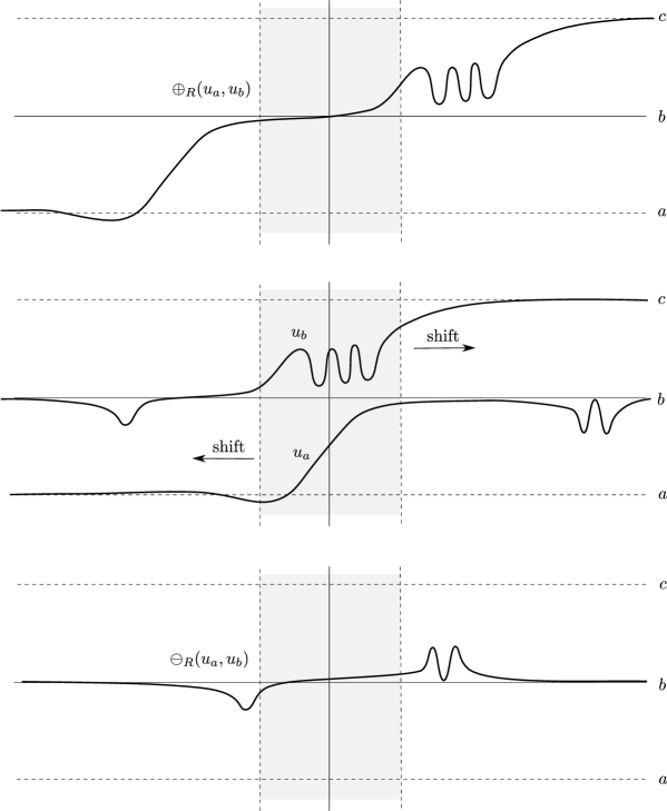
Figure 1. An example of plus gluing (i.e. pregluing) and minus gluing (i.e. anti-gluing) of two smooth paths $u_{a},u_{b}$ from $a$ to $b$ and from $b$ to $c$.

The topology on the space of broken and unbroken trajectories $\widetilde{\mathcal{B}}$ is now constructed by viewing the pregluing map as map to the quotient $\scriptstyle\mathcal{B}_{a}^{c}$/$\scriptstyle{\rm Aut}$, extending this map to gluing parameter $R=\infty$ by $(\infty,u_{a},u_{b})\mapsto\bigl{(}[u_{a}],[u_{b}]\bigr{)}$, and requiring this extended pregluing map to be open. In other words, a basis of open sets in $\widetilde{\mathcal{B}}$ is given by images under the extended pregluing map of open subsets of product type

$${\mathcal{U}}:=(R_{0},\infty]\times\mathcal{H}_{a}^{b}\times\mathcal{H}_{b}^{c}\;\subset\;(0,\infty]\times\bigl{(}\phi_{a}^{b}+{\mathcal{C}}^{1}(\mathbb{R},\mathbb{R}^{n})\bigr{)}\times\bigl{(}\phi_{b}^{c}+{\mathcal{C}}^{1}(\mathbb{R},\mathbb{R}^{n})\bigr{)}.$$

Here the ambient space on the right can be equipped with a scale smooth structure (with boundary) by replacing ${\mathcal{C}}^{1}(\mathbb{R},\mathbb{R}^{n})$ with a scale of weighted Sobolev spaces, as mentioned above, and by fixing a homeomorphism $[0,1)\cong(0,\infty]$ that identifies the boundaries $0$ and $\infty$. The latter is the notion of a gluing profile, which in polyfold theory is usually chosen as the exponential profile

(5) $$[0,1)\;\to\;(0,\infty],\qquad\tau\;\mapsto\;e^{1/\tau}-e.$$

The choice of the exponential gluing profile in particular ensures that the following constructions extend scale smoothly to the boundary. One could also hope to obtain a chart for $\widetilde{\mathcal{B}}$ near the broken path $([\gamma_{a}],[\gamma_{b}])$ from the map

(6) $$\Phi:\mathcal{U}\to\widetilde{\mathcal{B}}\qquad(R,u_{a},u_{b})\mapsto\begin{cases}[\oplus_{R}(u_{a},u_{b})]&;R<\infty,\\ ([u_{a}],[u_{b}])&;R=\infty.\end{cases}$$

Although $\Phi|_{\{R<\infty\}}$ is an sc-smooth map to $\scriptstyle{\mathcal{B}}_{a}^{c}$/$\scriptstyle\operatorname{Aut}$, it is far from being a local homeomorphism since it is not even a bijection except for its restriction to $\{R=\infty\}$. To see this, observe that for fixed $R<\infty$, the two maps $\oplus_{R}(u_{a},u_{b})$ and $\oplus_{R}(u_{a}+v_{+},u_{b}+v_{-})$ are equal whenever $v_{\pm}$ have support in a sufficiently small neighborhood of $\pm\infty$. At this point the core idea of polyfold theory arises: obtain a chart by restricting $\Phi$ to an appropriate subset of ${\mathcal{U}}$, which is then used as a local model for the scale smooth structure on $\widetilde{\mathcal{B}}$. In other words, we aim to achieve the following:

1. Find a subset $\mathcal{K}\subset\mathcal{U}$ for which $\Phi\big{|}_{\mathcal{K}}$ is a homeomorphism to its image.

2. Equip sets $\mathcal{K}$ of this type with a notion of scale smooth structure.

We will see that this can be achieved by describing ${\mathcal{K}}$ as the image of a retraction on ${\mathcal{U}}$. Moreover, this retraction will appear naturally from the idea of keeping track of the information lost during pregluing for $R<\infty$. This is accomplishved via the so-called anti-gluing map $\ominus_{R}$, which is given by a complementary interpolation of the same shifts as in the pregluing map $\oplus_{R}$. More specifically, the combination of both maps is given by a pair of reparametrizations together with multiplication by an invertible matrix of cutoff functions:

$$\left(\begin{matrix}\oplus_{R}(u_{a},u_{b})\\ \ominus_{R}(u_{a},u_{b})\end{matrix}\right)=\left(\begin{matrix}\beta&1-\beta\\ \beta-1&\beta\end{matrix}\right)\left(\begin{matrix}u_{a}(\cdot+{\textstyle\frac{R}{2}})\\ u_{b}(\cdot-{\textstyle\frac{R}{2}})\end{matrix}\right).$$

For each fixed $R<\infty$, this is a bijection by invertibility of the matrix at every $t\in\mathbb{R}$. In fact, one can check that it gives rise to an sc-smooth diffeomorphism

$$\boxplus:\{(R,u_{a},u_{b})\in\mathcal{U}\,|\,R<\infty\} \;\to\;\text{\raise 4.30554pt\hbox{$\mathcal{B}_{a}^{c}\!$}\big{/}\lower 4.30554pt\hbox{$\!{\rm Aut}$}}\times{\mathcal{C}}^{1}(\mathbb{R},\mathbb{R}^{n})$$

$$(R,u_{a},u_{b}) \;\mapsto\;\boxplus_{R}(u_{a},u_{b}):=\big{(}[\oplus_{R}(u_{a},u_{b})],\ominus_{R}(u_{a},u_{b})\big{)}.$$

Moreover, in appropriate charts for domain and target, each $\boxplus_{R}$ can be viewed as linear isomorphism ${\rm T}_{0}{\mathcal{V}}_{a}^{b}\times{\rm T}_{0}{\mathcal{V}}_{b}^{c}\to{\rm T}_{0}{\mathcal{V}}_{a}^{c}\times{\mathcal{C}}^{1}(\mathbb{R},\mathbb{R}^{n})$, which shows that $\ker\ominus_{R}$ is a complement to $\ker\oplus_{R}$. This achieves the first aim and gives an approach to the second:

1. The map $\Phi|_{\mathcal{K}}$ in (6) restricts to a bijection on

   $$\mathcal{K}:=\{(R,u_{a},u_{b})\subset\mathcal{U}\,|\,\ominus_{R}(u_{a},u_{b})=0\;\text{or}\;R=\infty\}.$$

   To check that $\Phi|_{\mathcal{K}}$ is a homeomorphism, one can use the observation that $(R,u_{a},u_{b})=\Phi^{-1}([v])$ is the unique solution of $\boxplus_{R}(u_{a},u_{b})=\bigl{(}[v],0\bigr{)}$.

2. After possibly shrinking $\mathcal{U}$, the latter gives rise to a description of the set $\mathcal{K}$ as fixed point set of the sc-smooth map

   $$r:{\mathcal{U}}\to{\mathcal{U}},\qquad r(R,u_{a},u_{b})=\begin{cases}\boxplus_{R}^{-1}\bigl{(}[\oplus_{R}(u_{a},u_{b})],0\bigr{)}&;R<\infty,\\ (R,u_{a},u_{b})&;R=\infty.\end{cases}$$

   In fact, this map satisfies the retraction property $r\circ r=r$ since for $R<\infty$ it is of the form $\boxplus_{R}^{-1}\circ\operatorname{pr}\circ\boxplus_{R}$, with $\operatorname{pr}(u,v):=(u,0)$ satisfying $\operatorname{pr}\circ\operatorname{pr}=\operatorname{pr}$. In particular, $\mathcal{K}=r(\mathcal{U})$ is an sc-retract; that is, it is the image of an sc-smooth retraction.

To accomplish our aims, it remains to show that $\mathcal{K}$ carries a meaningful notion of scale smoothness. In other words, we need a notion of scale-differentiability for maps $\Psi:\mathcal{K}\to\mathbb{F}$ to some other sc-Banach space $\mathbb{F}$. The notion of sc-continuity for such maps is naturally given since $\mathcal{K}$ carries an sc-topology induced from $\mathcal{U}$. The notion of sc¹ from scale calculus is also well defined if $\mathcal{K}$ is an open subset of an sc-Banach space. However, in our Morse theory example $\mathcal{K}$ has empty interior. Since $r\big{|}_{\mathcal{K}}=\operatorname{id}_{\mathcal{K}}$, a natural extension of $\Psi$ to a map from an open subset of an sc-Banach space is $\Psi\circ r:{\mathcal{U}}\to{\mathbb{F}}$. We can then define the map $\Psi:\mathcal{K}\to\mathbb{F}$ to be sc^k if and only if the map $\Psi\circ r:\mathcal{U}\to\mathbb{F}$ is sc^k. Similarly, we define the tangent spaces ${\rm T}_{k}{\mathcal{K}}$ as fixed point set of the linearized retraction ${\rm d}_{k}r$. These definitions makes sense (e.g. satisfy the chain rule and depend only on ${\mathcal{K}}$, not the choice of $r$) due to the retraction property $r\circ r=r$. In particular, the latter implies that the differential ${\rm d}r={\rm d}r\circ{\rm d}r$ is a retraction as well, so that the tangent bundle of an sc-retract is an sc-retract itself. This establishes a notion of scale smooth structure on ${\mathcal{K}}$, as aimed for in (ii). Further details can be found in Example 5.1.6.

From this Morse theory example, we see the utility of an sc-smooth retraction $r:\mathcal{U}\to\mathcal{U}$, which both characterizes the subset $\mathcal{K}=r({\mathcal{U}})$ on which a homeomorphic chart map $\Phi$ is defined, and provides a means to establish the notion of sc-differentiability on this subset. Such sc-smooth maps satisfying the retraction property $r\circ r=r$ are called sc-smooth retractions, and their images are called sc-retracts. These sc-retracts, together with a homeomorphism $\Phi:{\mathcal{K}}\to\widetilde{\mathcal{B}}$, form the local models of M-polyfolds. That is, an M-polyfold is a topological space $\widetilde{\mathcal{B}}$ that is locally homeomorphic to sc-retracts, such that the transition maps $\Phi^{-1}\circ\Phi^{\prime}:{\mathcal{K}}^{\prime}\to{\mathcal{K}}$ are sc-smooth in the sc-retract sense that $\Phi^{-1}\circ\Phi^{\prime}\circ r^{\prime}:{\mathcal{U}}^{\prime}\to{\mathcal{U}}$ is sc-smooth. The above outline can be fleshed out to prove that $\widetilde{\mathcal{B}}$ is an M-polyfold.

In suitable coordinates, the sc-smooth retraction for Morse theory introduced above, and in fact all sc-retractions arising in applications to date, have a rather specific form, namely

$$r:[0,1)^{k}\times\mathbb{E}\to[0,1)^{k}\times\mathbb{E}\qquad\text{given by}\qquad r(v,e)=(v,\pi_{v}e),$$

where $\mathbb{E}$ is an sc-Banach space, $v$ is thought of as a gluing parameter, and $\pi_{v}:\mathbb{E}\to\mathbb{E}$ is a family of linear projections. Note that the sc-smoothness conditions on $r$ do not require $v\mapsto\pi_{v}$ to be continuous in the operator topology, but just “pointwise” as map $(v,e)\mapsto\pi_{v}e$. This allows the image $\pi_{v}{\mathbb{E}}$ to jump in dimension as $v$ varies. Such retractions (given by a family of projections) are called splicings; the induced sc-retracts are called splicing cores; and they were used as local models for M-polyfolds in the early polyfold literature; c.f. [HWZ1, HWZ2, HWZ3].

In order to achieve the ultimate goal of describing the compactified Morse moduli space $\overline{\mathcal{M}}$ as the zero set of a section $\tilde{\sigma}:\widetilde{\mathcal{B}}\to\widetilde{\mathcal{E}}$ in a bundle that is sufficiently rich for a regularization theorem similar to Theorem 2.1.1, it remains to find a suitable notion of Fredholm sections in M-polyfold bundles. Here a notion of finite dimensional kernels and cokernels with constant index is necessary in order to have any hope for the zero set of a transverse section to be a finite dimensional manifold. However, note that in the Morse theory example, based on our expectation of what its zero set should be, the section in the pregluing chart must roughly have the form

$$\tilde{\sigma}(R,u_{a},u_{b})=\begin{cases}\bigl{(}\frac{{\rm d}}{{\rm d}t}\bigl{(}\oplus_{R}(u_{a},u_{b})\bigr{)}-\nabla f\bigl{(}\oplus_{R}(u_{a},u_{b})\bigr{)}\bigr{)}&;R<\infty\\ \bigl{(}\frac{{\rm d}}{{\rm d}t}u_{a}-\nabla f(u_{a}),\frac{{\rm d}}{{\rm d}t}u_{b}-\nabla f(u_{b})\bigr{)}&;R=\infty.\end{cases}$$

More specifically, the bundle $\widetilde{\mathcal{E}}\to\widetilde{\mathcal{B}}$ must have fibers isomorphic to ${\mathcal{C}}^{0}(\mathbb{R},\mathbb{R}^{n})$ over points such as $[\oplus_{R}(u_{a},u_{b})]$ in the interior of $\widetilde{\mathcal{B}}$, and it must have fibers isomorphic to ${\mathcal{C}}^{0}(\mathbb{R},\mathbb{R}^{n})\times{\mathcal{C}}^{0}(\mathbb{R},\mathbb{R}^{n})$ over broken trajectories such as $\bigl{(}[u_{a}],[u_{b}]\bigr{)}$. This can be achieved by constructing $\widetilde{\mathcal{E}}$ from pregluing maps along the same lines as for $\widetilde{\mathcal{B}}$. An important feature of this construction is that, roughly speaking, the fibers of $\widetilde{\mathcal{E}}$ jump in the same way as the tangent space ${\rm T}\widetilde{\mathcal{B}}$. In turn, this will allow for a meaningful Fredholm theory.

To define the notion of a scale Fredholm section, one could try to proceed along the lines of the construction of a scale smooth structure on an sc-retract ${\mathcal{K}}=r({\mathcal{U}})$. Note however that the linearization of $\tilde{\sigma}\circ r$ has infinite dimensional kernel as soon as ${\rm d}r$ does, which in the Morse theory example is the case whenever $R<\infty$. At the same time, if ${\mathcal{K}}^{\prime}$ is the sc-retract modeling the bundle ${\mathcal{E}}$, then ${\rm T}{\mathcal{K}}^{\prime}$ has infinite codimension in each fiber over $R<\infty$. Polyfold theory obtains a Fredholm theory by introducing the notion of a filled section, which in local charts is given as an sc-smooth extension $\overline{\sigma}:{\mathcal{U}}\to{\mathcal{U}}^{\prime}$ of the section $\tilde{\sigma}:{\mathcal{K}}\to{\mathcal{K}}^{\prime}$ to open subsets of sc-Banach spaces. The filled section is required to have the same zero set $\overline{\sigma}^{-1}(0)=\tilde{\sigma}^{-1}(0)$ as the original section, and to not contribute to the Fredholm index. In the setting of splicings, this means that the bundle splicing has the form

$$\rho:[0,1)^{k}\times\mathbb{E}\times{\mathbb{F}}\to[0,1)^{k}\times\mathbb{E}\times{\mathbb{F}},\qquad\rho(v,e,f)=(v,\pi_{v}e,\Pi_{v}f),$$

so that the fibers of $\widetilde{\mathcal{E}}\to\widetilde{\mathcal{B}}$ are given by $\operatorname{im}\Pi_{v}$ over $\{v\}\times\operatorname{im}\pi_{v}$, and there is an sc-smooth family of isomorphisms $\ker\Pi_{v}\cong\ker\pi_{v}$ between the kernels of the two splicings, as the gluing parameter $v$ varies. Such fillers can typically be constructed via the full gluing map $\widetilde{\boxplus}=([\widetilde{\oplus}],\widetilde{\ominus})$, where the nonlinear PDE must naturally be applied in the first factor, and a linearized PDE provides an isomorphism that acts on the second factor.

Based on these Fredholm notions in the context of scale-calculus and sc-retracts, one can then develop a perturbation and stability theory for scale Fredholm sections, which culminates in the Regularization Theorem 2.1.6 stated above.

3. Road maps for regularization approaches

In this section we compare the polyfold approach to regularizing moduli spaces to the geometric and virtual approaches in order to exhibit how the classical ingredients (compactness, quotienting by reparametrizations, Fredholm theory, gluing, etc.) are present in each of the approaches but with changing order and significance. We will outline the basic steps in each of these approaches via the example of Morse theory, and we do so using the setup from Examples 1.0.1 and  2.1.3. In more general abstract terms, we are discussing the regularization of a compactification $\overline{\mathcal{M}}$ of a moduli space ${\mathcal{M}}$, given by the solutions to a PDE modulo the reparametrization action of an automorphism group $\operatorname{Aut}$. Here and throughout, we will assume that $\operatorname{Aut}$ acts freely on the space of solutions, which we recall is always the case in Morse theory.

For a more detailed account of Morse theory along these lines, see [Sc1, AD]. Note however that the regularization of the Morse moduli spaces does not actually require their study as moduli spaces of a PDE. Rather, an entirely finite dimensional setup as spaces of trajectories under a smooth flow map yields the regularization as manifolds with boundaries and corners most effectively, e.g. [W1].

3.1. The geometric approach

In this section we describe techniques that obtain transversality by perturbing (or exploiting) geometric structures in the moduli problem; we call such techniques the “geometric approach.” In the case of Morse theory, the given moduli problem is the compactified Morse moduli space $\overline{\mathcal{M}}$ for a fixed Morse function $f:X\to\mathbb{R}$ and any Riemannian metric $g$ on $X$. This moduli space decomposes into (not necessarily connected) components $\overline{\mathcal{M}}(x_{-},x_{+})$ of (possibly broken) Morse trajectories between pairs of critical points $x_{\pm}\in\operatorname{Crit}f$. The goal of regularization is to replace $\overline{\mathcal{M}}$ by a regularized space $\overline{\mathcal{M}}\,\!^{\prime}$, which is a manifold with boundary and corners with components $\overline{\mathcal{M}}\,\!^{\prime}(x_{-},x_{+})$, whose first boundary stratum (excluding the higher corner strata) is a fiber product of its interior ${\mathcal{M}}^{\prime}\subset\overline{\mathcal{M}}\,\!^{\prime}$ with itself. In particular, it should have the form:

$$\partial\overline{\mathcal{M}}\,\!^{\prime}\;=\;{\mathcal{M}}^{\prime}\underset{\scriptscriptstyle\operatorname{Crit}f}{\times}{\mathcal{M}}^{\prime}\;=\;{\textstyle\bigcup_{x_{-},x,x_{+}\in\operatorname{Crit}f}}{\mathcal{M}}^{\prime}(x_{-},x)\times{\mathcal{M}}^{\prime}(x,x_{+}).$$

The signed count of the $0$-dimensional component of $\overline{\mathcal{M}}\,\!^{\prime}$ then defines the Morse differential $\partial$, and the boundary structure of the $1$-dimensional component establishes $\partial\circ\partial=0$. An additional step is then needed to prove independence of the induced Morse homology from both the choice of regularization $\overline{\mathcal{M}}\,\!^{\prime}$ and the choice of $(f,g)$. For other moduli problems, we write ${\mathcal{M}}^{\prime}\tilde{\times}{\mathcal{M}}^{\prime}$ for analogous fiber products, even if we expect the regularized moduli space to have no boundary (which is the case in Gromov-Witten). The basic order of constructions in geometric approaches is: 1) transversality, 2) quotient, 3) gluing; where reduction to finite dimensions occurs after transversality is achieved. Such constructions can be roughly broken down into the following eight steps – with adjustments in the case of “codimension 2 gluing” discussed later.

• Fredholm setup: Set up the PDE (e.g. gradient flow equation $\frac{{\rm d}}{{\rm d}t}\gamma-\nabla f=0$) as smooth section $\sigma:{\mathcal{B}}\to{\mathcal{E}}$ of a Banach space bundle ${\mathcal{E}}\to{\mathcal{B}}$ over a Banach manifold ${\mathcal{B}}$ of maps (e.g. $\gamma:\mathbb{R}\to X$ with suitable convergence to critical points). This section should be Fredholm in the sense that the linearizations ${\rm D}_{b}\sigma:{\rm T}_{b}{\mathcal{B}}\to{\mathcal{E}}_{b}$ at zeros $b\in\sigma^{-1}(0)$ are Fredholm operators. Moreover, the section $\sigma$ will be equivariant under the action of the automorphism group ${\rm Aut}$ on ${\mathcal{E}}\to{\mathcal{B}}$, so that the uncompactified moduli space is given as quotient of the zero set ${\mathcal{M}}=\sigma^{-1}(0)/{\rm Aut}$.

• Geometric perturbations: Find a family of smooth sections $(p:{\mathcal{B}}\to{\mathcal{E}})_{p\in{\mathcal{P}}}$ parametrized by a Banach manifold ${\mathcal{P}}$, with the following properties.

  1. For each $p\in{\mathcal{P}}$ the perturbed solution space $(\sigma+p)^{-1}(0)$ is invariant under the action of $\operatorname{Aut}$. (Usually this is achieved by using $\operatorname{Aut}$-equivariant sections $p$.)

  2. For each $p\in{\mathcal{P}}$ the perturbed solution space $(\sigma+p)^{-1}(0)$ has the same compactification properties as the unperturbed space $\sigma^{-1}(0)$.

  3. The “universal moduli space” $\widehat{\mathcal{M}}:=\bigl{\{}(b,p)\in{\mathcal{B}}\times{\mathcal{P}}\,\big{|}\,s(b)+p(b)=0\bigr{\}}$ is cut out transversely and has the structure of a Banach manifold. That is, for each $(b,p)\in\widehat{\mathcal{M}}$ we have a surjective linearized operator ${\rm T}_{b}{\mathcal{B}}\times{\rm T}_{p}{\mathcal{P}}\to{\mathcal{E}}_{b}$, given by $(\xi,\eta)\mapsto{\rm D}_{b}(s+p)(\xi)+\eta(b)$.

  (For Morse theory, the perturbations could be $p(\gamma)=\nabla f(\gamma)-\nabla^{\prime}f(\gamma)$, where $\nabla^{\prime}$ is the gradient with respect to another metric $g^{\prime}$ on $X$.)

• Sard-Smale Theorem (automatic): Given a family of perturbations ${\mathcal{P}}$ as described, the Sard-Smale theorem guarantees a comeagre set ${\mathcal{P}}^{\rm reg}\subset{\mathcal{P}}$ of regular values of the canonical projection $\operatorname{pr}:\widehat{\mathcal{M}}\to\mathcal{P}$. Moreover, a little functional analysis (see [MS, Lemma A.3.6]) shows that for $p\in{\mathcal{P}}^{\rm reg}$ the perturbed section $\sigma_{p}:=\sigma+p$ is transverse to the zero section, yet it is still ${\rm Aut}$-equivariant. Hence, by the implicit function theorem, $\sigma_{p}^{-1}(0)\subset{\mathcal{B}}$ is a smooth submanifold of finite dimension on which $\operatorname{Aut}$ acts, and the dimension is given by the Fredholm index. (For Morse theory, this would pick out the metrics that satisfies the Morse-Smale condition: transversal intersection of stable and unstable manifolds.)

• Quotient: Check that the action of ${\rm Aut}$ on $\sigma_{p}^{-1}(0)$ is smooth, free, and properly discontinuous. Then the moduli space ${\mathcal{M}}_{p}:=\sigma_{p}^{-1}(0)/{\rm Aut}$ is a smooth manifold.

• Gluing: Construct a gluing map $\tilde{\oplus}:(R_{0},\infty)\times{\mathcal{M}}_{p}\tilde{\times}{\mathcal{M}}_{p}\hookrightarrow{\mathcal{M}}_{p}$ that is an embedding (e.g. for fixed critical points it should map ${\mathcal{M}}_{p}(x_{-},x)\times{\mathcal{M}}_{p}(x,x_{+})$ to paths parametrized by the gluing parameter $(R_{0},\infty)$ in ${\mathcal{M}}_{p}(x_{0},x_{+})$). The construction of $\tilde{\oplus}$ involves a pregluing map $\oplus:(R_{0},\infty)\times\sigma_{p}^{-1}(0)\tilde{\times}\sigma_{p}^{-1}(0)\to{\mathcal{B}}$ similar to (4), and an implicit function theorem to determine exact solutions.

  Small print on corners: This technique is usually only applied to glue $0$-dimensional components or compact subsets of the fiber product. More generally, to give a higher dimensional moduli space the structure of a manifold with boundary and corners one would have to construct higher gluing maps $\tilde{\oplus}:(R_{0},\infty)^{\ell}\times\tilde{\times}^{\ell+1}{\mathcal{M}}_{p}\hookrightarrow{\mathcal{M}}_{p}$ which cover the overlap of the basic gluing maps, and one would also need to check smoothness of transition maps and verify a cocycle condition.

• Coherence: Ensure that the choice of perturbation $p$ can be made “coherently”; that is, check that perturbations are compatible with the gluing map. Consequently steps 2) - 5) are interwoven, and they are potentially organized by a hierarchy of connected components of $\overline{\mathcal{M}}$, such as by the difference in Morse indices of $x_{\pm}$ for the components $\overline{\mathcal{M}}(x_{-},x_{+})$.

• Compactness: Check that the complement of the gluing image, ${\mathcal{M}}_{p}\setminus\operatorname{im}\tilde{\oplus}$, is compact. Then construct a compactification of the perturbed moduli space as $\overline{\mathcal{M}}_{p}=\bigl{(}{\mathcal{M}}_{p}\sqcup(R_{0},\infty]\times{\mathcal{M}}_{p}\tilde{\times}{\mathcal{M}}_{p}\bigr{)}/\tilde{\oplus}$. After choosing a homeomorphism $(R_{0},\infty]\cong[0,1)$, this yields a smooth manifold with boundary $\{\infty\}\times{\mathcal{M}}_{p}\tilde{\times}{\mathcal{M}}_{p}$.

  Small print on corners: If the gluing maps have overlaps, e.g. due to higher gluing maps, then one would have to add their domains $(R_{0},\infty]^{\ell}\times\tilde{\times}^{\ell+1}{\mathcal{M}}_{p}$ to $\overline{\mathcal{M}}_{p}$ and take the quotient by all gluing maps. However, this requires the cocycle condition. If this can be satisfied, then $\{\infty\}^{\ell}\times\tilde{\times}^{\ell+1}{\mathcal{M}}_{p}$ forms the $\ell$-th corner stratum of $\overline{\mathcal{M}}_{p}$.

• Invariance: Prove that the algebraic structures (e.g. the Morse chain complex) arising from different choices in the previous steps, in particular the choice of perturbation, are equivalent in an appropriate sense (e.g. chain homotopic). This usually involves the construction of a cobordism from a moduli space involving a homotopy of choices.

When applied to a moduli space of pseudoholomorphic curves, Steps 1 – 3 remain unchanged, with ${\mathcal{B}}$ consisting of maps from a fixed Riemann surface $\Sigma$, possibly with additional marked points and possibly varying complex structure on $\Sigma$. (Note that we cannot work with a Deligne-Mumford type space of Riemann surfaces modulo biholomorphisms, since the corresponding space of maps and surfaces does not have a natural Banach manifold structure; see [MW, §3.2].) Then the section $\sigma$ is given by the Cauchy-Riemann operator – but possibly with further conditions on (for example) the evaluation map at the marked points. Finally, $\operatorname{Aut}$ is the group of holomorphic automorphisms of the underlying complex curve $\Sigma$. (In the case of varying complex structures, one usually reduces the space of complex structures so that there are no further automorphisms.) Here the requirement that $\operatorname{Aut}$ acts freely on $\sigma_{p}^{-1}(0)$ is rather restrictive since it excludes perturbed solutions $u$ with nontrivial isotropy, that is $\phi\neq\operatorname{id}_{\Sigma}$ such that $u\circ\phi=u$. If $\operatorname{Aut}$-equivariant transversality can be achieved in Step 2, then nontrivial finite isotropy groups could be allowed in Step 4 with the result of $\sigma_{p}^{-1}(0)/{\rm Aut}$ being an orbifold. However, holomorphic curves with nontrivial isotropy also lack the injectivity properties that are needed for the common approaches to achieving transversality (P3); see Remark 3.1.1. In special cases, it might be possible to overcome this transversality issue by enriching the geometric approach with “groupoid” or “multivalued perturbation” methods.

More abstractly, the existence of perturbations as required in Step 2 is not a general fact for equivariant Fredholm sections, since many useful classes of perturbations (like the class of compact perturbations) need not preserve the compactness properties of the solution set for general non-linear Fredholm problem. Furthermore, the equivariance and transversality properties (P1) and (P3) are often mutually exclusive requirements.

For the Cauchy-Riemann operator $\bar{\partial}_{J}$, the natural geometric structure to perturb is the given almost complex structure $J$. This means that the perturbations $p\in{\mathcal{P}}$ are of the form $p(u)=\frac{1}{2}(J-J^{\prime}){\rm d}u\circ j$ for some other almost complex structure $J^{\prime}$. From the abstract functional analytic point of view, this is a perturbation of the same order as the differential operator, so the Fredholm property is preserved only by a homotopy of semi-Fredholm operators (using the elliptic estimates for each Cauchy-Riemann operator together with the connectedness of the space of compatible almost complex structures). For the compactness property (P2) we need to use our geometric understanding of $J$-holomorphic curves for any compatible $J$ to see that Gromov compactness persists. However, comparing the requirements for equivariance (P1) and transversality (P3), as in the following remark, one sees that almost complex structures only provide the required set of perturbations if, roughly speaking, the pseudoholomorphic maps are somewhere injective along any orbit of a point in the domain $\Sigma$ under the automorphism action. This follows from the invariance of $J$ along $\operatorname{Aut}$-orbits in $\Sigma$. Further common geometric perturbations are Hamiltonian vector fields. These are lower order (compact) perturbations, which otherwise are used in close analogy to the perturbations in the almost complex structure.

Remark 3.1.1 (Small print on injectivity requirements).

Let us semi-formally unravel the equivariance property (P1) and the universal transversality property (P3) when we perturb by a space ${\mathcal{J}}$ of possibly domain dependent compatible almost complex structures $J:\Sigma\to{\mathcal{J}}(M,\omega)$.

1. Invariance of the solution set $\{u:\Sigma\to M\,|\,\bar{\partial}_{J}u=0\}$ under reparametrization by an automorphism $\phi:\Sigma\to\Sigma$ requires $J:\Sigma\to{\mathcal{J}}(M,\omega)$ to satisfy $J\circ\phi=J$. In particular, $J(z)$ must be constant along orbits $z\in\{\phi(z_{0})\,|\,\phi\in\operatorname{Aut}\}$ of the automorphism group, and the same holds for infinitesimal variations $Y\in{\rm T}_{J}{\mathcal{J}}$.

2. Transversality of the universal moduli space at $\bar{\partial}_{J}u=0$ requires, roughly speaking, that the only element $\eta\in\ker({\rm D}_{u}\bar{\partial}_{J})^{*}$ in the kernel of the dual linearized Cauchy-Riemann operator that satisfies $\int_{\Sigma}\langle\,\eta(z)\circ j,Y(z,u(z)){\rm d}_{z}u\,\rangle=0$ for all $Y\in{\rm T}_{J}{\mathcal{J}}$ is $\eta=0$.

Assuming $\eta(z_{0})\neq 0$ in contradiction to (P3), linear algebra guarantees the existence of $Y\in{\rm T}_{J}{\mathcal{J}}$ such that $\langle\,\eta(z_{0})\circ j,Y(z_{0},u(z_{0})){\rm d}_{z_{0}}u\,\rangle>0$, as long as ${\rm d}_{z_{0}}u\neq 0$. We then wish to cut off $Y$ near $(z_{0},u(z_{0}))\in\Sigma\times M$ so that the integrand $\langle\,\eta(z)\circ j,Y(z,u(z)){\rm d}_{z}u\,\rangle$ remains positive for all $z\in\Sigma$. However, $Y$ is forced by (P1) to be constant along the $\operatorname{Aut}$-orbit through $z_{0}$, so that we need to use cutoff in $M$ near $u(z_{0})$. The latter can only be guaranteed if we have $u(\phi(z_{0}))\neq u(z_{0})$ for all $\phi(z_{0})\neq z_{0}$; in other words, the $J$-holomorphic map $u$ needs to be injective along the orbit through $z_{0}$, and additionally, $z_{0}$ can not be a singular point of $u$.

On the other hand, we usually have unique continuation for the Cauchy-Riemann equation along $\operatorname{Aut}$-orbits, due to the invariance of $J$ along these $\operatorname{Aut}$-orbits. For the dual linearized operator this means that for $({\rm D}_{u}\bar{\partial}_{J})^{*}\eta=0$ and $\eta|_{V}\equiv 0$ on some open subset $V\subset\Sigma$ we obtain $\eta_{{\rm Aut}\cdot V}\equiv 0$ on the orbit of $V$. Hence it suffices to have injectivity of $u$ and nonvanishing of ${\rm d}u$ somewhere along almost every $\operatorname{Aut}$-orbit in $\Sigma$. The most important cases are the following.

• For pseudoholomorphic spheres with zero, one, or two fixed marked points, the automorphism group acts transitively on $\Sigma=S^{2}$, so that it suffices to find some $z_{0}\in S^{2}$ with ${\rm d}_{z_{0}}u\neq 0$ and $u^{-1}(u(z_{0}))=u(z_{0})$. In fact, by [Mc, MS] the set of such “injective points” is dense unless $u$ is multiply covered. This is equivalent to the existence of some nontrivial Möbius transformation $\phi:S^{2}\to S^{2}$ for which $u\circ\phi=u$, which can be stated more elegantly by saying $u$ has a nontrivial isotropy group.

• For pseudoholomorphic disks with zero or one marked points on the boundary, it similarly suffices to have one “injective point”. However, there now exist nowhere injective disks that are not multiply covered, i.e. have trivial isotropy group. An example is the “lantern”: a disc mapping to $M=S^{2}$ with boundary on the equator that wraps two and a half times around the sphere.

• For Floer trajectories, i.e. pseudoholomorphic strips (disks with two marked points) or cylinders (spheres with two marked points, but with a Hamiltonian perturbation that breaks the $S^{1}$-symmetry), the automorphism group is $\mathbb{R}$. So it suffices to find for almost every $t_{0}\in[0,1]$ (or $t_{0}\in S^{1}$) a point $s_{0}\in\mathbb{R}$ with ${\rm d}_{(s_{0},t_{0})}u\neq 0$ and $u(s,t_{0})\neq u(s_{0},t_{0})$ for all $s\neq s_{0}$. In fact, unless the trajectory is constant (i.e.  $\partial_{s}u\equiv 0$), the set of such points $(s_{0},t_{0})$ is dense by [FHS].

Further injectivity requirements for the transversality of pseudholomorphic maps arise, for example in SFT, from invariance conditions for the almost complex structures on the target $M$. Apart from such cases, transversality can be obtained by this geometric Sard-Smale method for any stable domain $\Sigma$. (This excludes tori and spheres or disks with less than 3 marked points; where points in the interior of a disk count double.) However, any bubbling in a space of pseudholomorphic curves (i.e. blow-up of the gradient) leads to unstable sphere or disk components, so that this basic version of the geometric regularization approach is firmly restricted to cases in which bubbling can be a priori excluded – or at least the dimension of spaces of nowhere injective bubbles is controlled by underlying injective curves. The first prominent case considered aspherical symplectic manifolds, in which Floer [F1] excluded bubbles by their nonzero energy. This argument has a direct generalization to monotone settings [Oh], where a proportionality between energy and Fredholm index allows one to exclude sphere or disk bubbling in moduli spaces of small dimension. Finally, in semi-positive symplectic manifolds, the multiply covered spheres have to be localized on simple spheres, whose codimension in the moduli space is at least $2$, so that, for example, Gromov-Witten moduli spaces can be regularized to pseudo-cycles; see [MS].

Moving on to the compactness properties of spaces of pseudoholomorphic maps, the common singularity formations are “bubbling”, where energy concentrates, “breaking”, where energy escapes into noncompact ends of the domain or target, and the formation of “nodes” which might be allowed in the underlying space of Riemannian surfaces. With the exception of sphere bubbles and interior nodes, these can be compactified along the lines of Steps 4 - 6, leading to boundaries and corners, and thus invariance of solution counts only up to some algebraic equivalence as in Step 7. Sphere bubbling and interior nodes can also be treated analogously, although they give rise to interior points (or codimension $2$ points that do not contribute to the pseudo-cycle) of the compactified moduli space as follows.

• Gluing: Due to an extra rotation parameter at the node, the gluing map (for a single node) is of the form $\tilde{\oplus}:(R_{0},\infty)\times S^{1}\times{\mathcal{M}}_{p}\tilde{\times}{\mathcal{M}}_{p}\hookrightarrow{\mathcal{M}}_{p}$.

• Compactness: By choosing a homeomorphism from $\bigl{(}(R_{0},\infty)\times S^{1}\bigr{)}\cup\{\infty\}$ to the open unit disk, one could construct a smooth manifold in which sphere bubbles (or interior nodes) are interior points. However, smooth compatibility of the gluing maps is generally hard to achieve, so that this technique is mostly used to deduce compactness up to codimension $2$ singularities.

• Invariance: With the perturbed and compactified moduli spaces being closed (or pseudo-cycles), one obtains well defined counts of solutions (or more generally one obtains a well defined integral over the solution set) by regularizing moduli spaces that involve an interpolating $1$-parameter family of perturbations; in turn, such spaces provide a cobordism between a pair moduli spaces obtained from different choices of perturbation, and such a cobrodism then guarantees counts (or integrals) are independent of initial perturbation.

Finally, let us mention two more special cases of the geometric regularization approach. The simplest is the case of pseudoholomorphic curves of small genus with positive index in a four dimensional symplectic manifold, for which automatic transversality guarantees sujrectivity of the linearized Cauchy-Riemann operator for every choice of almost complex structure. This approach has been used successfully in a variety applications; see [Gr, HLS, We2].

An example with more general perturbations is the construction of spherical Gromov-Witten invariants developed in [CM]. (This approach was also used in [Fa] and recently generalized to the positive genus case in [Ge]; Ionel lays the foundations for a similar approach in [I].) Here the idea is to fix a Donaldson hypersurface in such a way that the marked points given by intersections with the hypersurface stabilize every pseudoholomorphic map in a given homology class. Letting ${\mathcal{B}}$ be a sufficiently small neighborhood of the pseudoholomorphic maps, one then obtains an $\operatorname{Aut}$-invariant map to a Deligne-Mumford space of marked Riemann surfaces. One can then work with a space of perturbations ${\mathcal{P}}$ that is given by families of almost complex structures over the Deligne-Mumford space. In other words, the almost complex structure $J(u)$ is no longer defined pointwise, but may depend on the position of the intersections of $u$ with the Donaldson hypersurface. This approach then yields regularizations in the form of pseudo-cycles, unique up to rational cobordism, and hence rational Gromov-Witten invariants.

3.2. The virtual approach

The analytic starting point of the “virtual approach” is the observation that the solution set of the Cauchy-Riemann operator restricted to a local slice of the ${\rm Aut}$-action (as in Remark 2.1.5) is homeomorphic to an open subset of the moduli space. Since this is a Fredholm section, one can find a finite dimensional reduction; in other words, one can find a section of a finite dimensional bundle and a homeomorphism from its zero set to an open subset of the moduli space. Alternatively, one could view this procedure as finding a finite dimensional obstruction bundle over an open subset of ${\mathcal{B}}/\operatorname{Aut}$ that covers the cokernel of the linearized Cauchy-Riemann operators. Both versions of this approach then aim to work in a finite dimensional category (either just for the fibers of the obstruction bundle or for both fibers and base in finite dimensional reductions) to associate a “virtual fundamental class” to the compactified moduli space $\overline{\mathcal{M}}$; for example, sometimes one aims to find a Čech homology class $[\overline{\mathcal{M}}]_{\kappa}\in\check{H}(\overline{\mathcal{M}};{\mathbb{Q}})$ induced by a special type of Kuranishi atlas $\kappa$ on $\overline{\mathcal{M}}$ as in [MW]. We base this exposition on the latter, and consequently we do not explicitly discuss obstruction bundle techniques, which would proceed along similar lines.

The overall structure of the virtual approach reorders the basic ingredients of the geometric approach from 1) transversality, 2) quotient, 3) gluing to 1) quotient, 2) transversality, 3) gluing, and it aims to reduce the problem to a finite dimensional setting as quickly as possible. A main feature of this approach is that it provides a natural setting for dealing with nonfree actions. Let us only note here that this introduces an additional finite group action, or groupoid structure, in the second of the following steps, and it additionally requires equivariance in the further steps.

• Compactness: Construct the compactified moduli space $\overline{\mathcal{M}}$ as a compact (usually metrizable) topological space containing ${\mathcal{M}}$ as well as ${\mathcal{M}}\tilde{\times}{\mathcal{M}}$, and which possibly contains higher fiber products.

• Quotient (local): View the uncompactified moduli space as subset ${\mathcal{M}}\subset{\mathcal{B}}/{\rm Aut}$ of the quotient space of maps as in the geometric approach, and for any $[u]\in{\mathcal{M}}$ find a local slice. That is, find a Banach submanifold ${\mathcal{B}}_{H}\subset{\mathcal{B}}$ such that $\operatorname{Aut}\times{\mathcal{B}}_{H}\to{\mathcal{B}}$ is a homeomorphism to an open subset. Since $\operatorname{Aut}$ generally does not act differentiably on infinite dimensional spaces of maps like ${\mathcal{B}}$, this requires a geometric construction as in Remark 2.1.5, for example.

• Fredholm setup and almost Transversality (local): Set up the PDE as a smooth Fredholm section $\sigma:{\mathcal{B}}_{H}\to{\mathcal{E}}|_{{\mathcal{B}}_{H}}$ of a Banach space bundle such that $\sigma^{-1}(0)$ is homeomorphic to an open neighborhood of the center, $[u]\in{\mathcal{M}}$, of the local slice. From this, and a choice of finite dimensional obstruction bundle $\widehat{E}\to{\mathcal{B}}_{H}$ that covers the cokernels of the linearized PDE, construct a finite dimensional reduction, which by definition is a smooth section $s:B\to E$ of a finite dimensional $E\to B$ over a manifold $B$ such that $s^{-1}(0)$ is homeomorphic to a neighborhood of $[u]\in{\mathcal{M}}$.

• Gluing (local): Construct finite dimensional reductions for the higher strata of $\overline{\mathcal{M}}$ from a gluing construction. The standard gluing analysis does not provide smooth sections $s:B\to E$ in this case, but an appropriate notion of stratified smoothness should suffice.

• Semi-local Transversality and Quotient compatibility (transition data): Establish compatibility of the local finite dimensional reductions by forming direct sums of the obstruction bundles near overlaps in $\overline{\mathcal{M}}$. This requires one to refine the choice of obstruction bundles in steps 3 and 4 such that they are transverse on the overlaps. The direct sum construction also involves pullbacks of the obstruction bundles by an action of ${\rm Aut}$, due to the changing local slices in step 2. To ensure smoothness and differentiability of the pullback bundles, specific geometric constructions of the obstruction bundles are needed.

• Kuranishi regularization (automatic): A general abstract theory associates a virtual fundamental class $[\overline{\mathcal{M}}]^{\rm vir}$ to any covering of $\overline{\mathcal{M}}$ by finite dimensional reductions that are suitably compatible. Roughly speaking, the Kuranishi charts and transition data form categories $\widetilde{B},\widetilde{E}$ and a functor $\widetilde{s}:\widetilde{B}\to\widetilde{E}$ so that $\overline{\mathcal{M}}$ is identified with the realization of the subcategory $|\widetilde{s}^{-1}(0)|$ (which by definition is the subspace of objects at which the section vanishes, modulo the equivalence relation generated by the morphisms). The abstract theory then aims to provide a class of perturbation functors $\widetilde{p}:\widetilde{B}\to\widetilde{E}$ such that $|(\widetilde{s}+\widetilde{p})^{-1}(0)|$ inherits the structure of a compact manifold, and that up to some type of cobordism is independent of $p$.

• Coherence: If $\overline{\mathcal{M}}$ consists of several components and an identification of the boundary $\partial[\overline{\mathcal{M}}]_{\mathcal{K}}$ with a fiber product $[\overline{\mathcal{M}}]_{\mathcal{K}}\tilde{\times}[\overline{\mathcal{M}}]_{\mathcal{K}}$ is desired, then steps 2 - 6 need to choose the local slices, obstruction bundles, and abstract perturbations “coherently”; in other words they much be chosen to be compatible with the gluing maps. (We note that, potentially, these interwoven steps can be organized by a hierarchy of connected components of $\overline{\mathcal{M}}$.)

• Invariance: Prove that the algebraic structures arising from different choices in the previous steps, in particular the choice of local slices and obstruction bundles, are equivalent. This involves the construction of a virtual fundamental chain on $[0,1]\times\overline{\mathcal{M}}$ from local finite dimensional reductions which reduce to two given choices on $\{0\}\times\overline{\mathcal{M}}$ and $\{1\}\times\overline{\mathcal{M}}$.

At present, the applicability of the virtual approach to pseudholomorphic curve spaces is being revisited. The recent [MW] discusses a number of fundamental analytic and topological issues in [FO, FOOO, LiT, LiuT] (one of which is discussed in Example 5.1.5), while itself only providing a theory for severely limited cases in which geometric methods are known to apply. Our hope is that a nontrivial convex span of all these publications should lead to a theory that is not only solid but also understood by more people than just the respective authors.

Assuming that a functional theory for the abstract regularization step 6 is established, the virtual approach does allow one to regularize more moduli problems, yet does not seem to eliminate repetitive work in the other steps. In particular, any application to a new moduli problem still requires some new geometric insight to find appropriate local slices in step 2 and obstruction bundles in step 3 that transform appropriately under the automorphism action; this is similar to finding a special set of perturbations in the geometric approach. The Fredholm setup in step 3 is also somewhat more complicated than in the geometric approach, since the local slice condition must be incorporated. Next, the gluing analysis in step 4 is exactly the same as that in the geometric approach, but the smoothness requirements on the finite dimensional reductions in fact require a more refined analysis than in some geometric regularizations, which merely construct a pseudocycle. Moreover, some additional technical work is required to obtain the transversality of obstruction bundles needed in step 5. Finally, coherence and invariance in steps 7 and 8 again require the same amount of work and sometimes nontrivial ideas as in the geometric approach.

Remark 3.2.1 (Relation between Kuranishi atlases and polyfold Fredholm sections).

A description of ${\overline{\mathcal{M}}}$ as the zero set of a Fredholm section in a polyfold bundle, as outlined in Section 3.3 below, is expected to induce an equivalence class of Kuranishi-type atlases for ${\overline{\mathcal{M}}}$. The rough idea is that this setting allows one to perform steps 1–5 of the virtual regularization scheme abstractly (or rather, they are already part of the polyfold setup). This requires choosing obstruction spaces that locally cover the cokernel; with different choices yielding equivalent atlases in the sense of having a common refinement (for details see e.g. [MW]).

In the case of trivial isotropy, the stabilization construction for classical Fredholm sections can be obtained, see for example in [CMS], and it yields a global finite dimensional reduction (also referred to as an atlas with one chart); in other words, ${\overline{\mathcal{M}}}$ can be described as the zero set of a single section of a finite dimensional bundle. In the case of nontrivial isotropy, and under the additional assumption that at every solution there exists a choice of obstruction space on which the isotropy group of the given point acts trivially, the above stabilization construction generalizes, and it yields a global finite dimensional reduction to a section of an orbi-bundle. To the best of the last author’s understanding, this assumption coincides with the notion of “semi-effective d-orbifold” for which regularization is discussed in [J]. In this case, however, the regularization in step 6 can be quoted directly from Theorem 2.1.1 or its generalization to orbibundles. Similarly, the Euler class approach of [Si] seems to go through under this additional assumption, and it yields a similar global finite dimensional reduction.

In the general case, [Y] proposes that finite dimensional reduction of Fredholm sections of polyfold bundles yields more general Kuranishi atlases with several charts. This resulting class of Kuranishi atlases should have well controlled transition maps which allow for a converse construction, which would yeild an equivalence between polyfold Fredholm sections and certain Kuranishi atlases.

3.3. The polyfold approach

The polyfold approach, just like the geometric one, aims to associate to a compactified moduli space $\overline{\mathcal{M}}$, a smooth compact manifold $\overline{\mathcal{M}}\,\!^{\prime}$, possibly with boundary $\partial\overline{\mathcal{M}}\,\!^{\prime}={\mathcal{M}}^{\prime}\tilde{\times}{\mathcal{M}}^{\prime}$, which is unique up to the appropriate notion of cobordism. In order to achieve this, and eliminate a lot of the repetitive work in the applications, this approach fundamentally changes the basic order of ingredients from 1) transversality, 2) quotient, 3) gluing in the geometric approach and 1) quotient, 2) transversality, 3) gluing in the virtual approach to the order 1) quotient, 2) gluing, 3) transversality, and remains in an infinite dimensional setting until transversality is achieved. The following eight steps provide an outline of the regularization procedure for a given moduli problem offered by the polyfold approach. [Additionally, in italics, we will compare each step to related constructions in the other approaches to demonstrate how significant amounts of technical work are automatized in the polyfold approach.]

• Compactness: Construct a (metrizable) topological space $\widetilde{\mathcal{B}}$ that contains the compactified moduli space $\overline{\mathcal{M}}$ as compact subset. Roughly speaking, $\widetilde{\mathcal{B}}$ can be obtained from the quotient space $\widetilde{\mathcal{B}}[0]:={\mathcal{B}}/\operatorname{Aut}$, which contains the moduli space ${\mathcal{M}}$ of smooth (i.e. non-nodal or unbroken) solutions of the PDE, by adding strata $\widetilde{\mathcal{B}}[\ell]$ of singular maps (e.g. $\ell$-fold broken, or with $\ell$ nodes) that need not satisfy the PDE, in the same way as $\overline{\mathcal{M}}$ is obtained from ${\mathcal{M}}$ by adding strata of singular solutions. These higher strata consist of large function spaces which will not, in general, solve the given PDE but will contain the compactification points of the moduli space, $\overline{\mathcal{M}}\setminus\mathcal{\mathcal{M}}$. [This is the same starting point as in the obstruction bundle version of the virtual approach. It is only slightly more complicated than topologizing the compactified moduli space $\overline{\mathcal{M}}$ in step 1 of the virtual approach and step 7 of the geometric approach.]

• Quotient (global): Give $\widetilde{\mathcal{B}}[0]={\mathcal{B}}/\operatorname{Aut}$ a scale smooth structure as a “scale Banach manifold” by finding local slices as in Remark 2.1.5. That is, find Banach submanifolds ${\mathcal{B}}_{H}\subset{\mathcal{B}}$ such that $\operatorname{Aut}\times{\mathcal{B}}_{H}\to{\mathcal{B}}$ is a homeomorphism to an open subset, and check that the transition maps are scale smooth. Do the same with each singular stratum $\widetilde{\mathcal{B}}[\ell]$, which is given by a fiber product of two or more copies of the main stratum, e.g. $\widetilde{\mathcal{B}}[1]\cong\widetilde{\mathcal{B}}[0]\tilde{\times}\widetilde{\mathcal{B}}[0]$. [The local slices are the same as those required in step 2 of the virtual approach. Their existence and scale smoothness follow from triviality of isotropy groups (which we assume throughout) and similar basic analytic properties of the action as those used to establish step 4 of the geometric approach.]

• Pregluing: Give the main stratum $\widetilde{\mathcal{B}}$ a generalized smooth structure near the strata of singular maps. In order to construct charts centered at once broken or nodal map in $\widetilde{\mathcal{B}}[1]$, use a pregluing map of the form $\oplus:{\mathcal{G}}^{*}\times{\mathcal{U}}_{0}\tilde{\times}{\mathcal{U}}_{1}\to\widetilde{\mathcal{B}}[0]$ for open sets ${\mathcal{U}}_{i}\subset\widetilde{\mathcal{B}}[0]$ (realized as local slices ${\mathcal{U}}_{i}\hookrightarrow{\mathcal{B}}$). Here the space of gluing parameters is ${\mathcal{G}}^{*}=(R_{0},\infty)$ in the case of a broken or boundary nodal map, whereas ${\mathcal{G}}^{*}=(R_{0},\infty)\times S^{1}$ for the case of an interior node. In either case, the pregluing map is extended by $\{\infty\}\times{\mathcal{U}}_{0}\tilde{\times}{\mathcal{U}}_{1}$ mapping to the corresponding broken or nodal maps in the singular stratum $\widetilde{\mathcal{B}}[1]\subset\widetilde{\mathcal{B}}$. We then give ${\mathcal{G}}:={\mathcal{G}}^{*}\cup\{\infty\}$ a smooth structure by “a choice of gluing profile,” which is a choice of identification with an interval $[0,1)\cong{\mathcal{G}}$ with $\{0\}\cong\{\infty\}$ in the boundary case, and an open disk with $\infty$ at the center in the interior case.

  To make up for the lack of injectivity of these pregluing maps, follow a “gluing and antigluing” procedure outlined in section 2.3, to form an sc-retract ${\mathcal{R}}\subset{\mathcal{G}}\times{\mathcal{U}}_{0}\tilde{\times}{\mathcal{U}}_{1}$, on which the restriction of $\oplus$ is a homeomorphism to an open subset of $\widetilde{\mathcal{B}}$. Analogously, construct such M-polyfold charts near the higher strata $\widetilde{\mathcal{B}}[\ell]$ of multiply broken or nodal maps in $\widetilde{\mathcal{B}}$ from pregluing maps $\oplus:{\mathcal{G}}^{\ell}\times\tilde{\times}^{i=\ell}_{i=0}{\mathcal{U}}_{i}\to\widetilde{\mathcal{B}}$ on multiple fiber products of local slices. In order to obtain scale smooth transition maps between these charts as well as the local slice charts arising from step 2, the safe choice is an exponential gluing profile as in (5). [This is a mild extension of the pregluing construction that provides the basis for an intricate Newton iteration in the gluing analysis of step 5 (or 5’) in the geometric approach and step 4 in the virtual approach. The novelty is in the interpretation as chart maps. The construction of these charts and scale smoothness of transition maps should usually be obtained by combining basic local building blocks in the literature with a Deligne-Mumford theory for the space of underlying domains.]

• Fredholm setup: After gathering the compatible charts constructed in steps 2 and 3 to an M-polyfold structure on $\widetilde{{\mathcal{B}}}$, analogously construct an M-polyfold bundle $\widetilde{{\mathcal{E}}}\to\widetilde{{\mathcal{B}}}$ such that the PDE (e.g. the gradient flow or Cauchy-Riemann operator) forms a section $\sigma:\widetilde{{\mathcal{B}}}\to\widetilde{{\mathcal{E}}}$ with $\sigma^{-1}(0)=\overline{\mathcal{M}}$. Check that the section $\sigma$ is a scale smooth polyfold Fredholm section. [The bundle $\widetilde{\mathcal{E}}$ could be constructed in one stroke with the ambient space $\widetilde{\mathcal{B}}$ by adding fibers that are essentially given by the requirement of the PDE forming a section. This bundle as well as the regularity and Fredholm property of the section should again usually be obtained from patching together local building blocks for which Fredholm properties are established in the literature. For regular domains (smooth, connected Riemann surfaces), the Fredholm property is essentially the same as in step 1 of the geometric approach and step 3 of the virtual approach. For nodal or broken domains, the polyfold Fredholm property formalizes part of the gluing analysis, namely it essentially follows from the quadratic estimates that are required in the gluing analysis of the other approaches.]

• Transversality (automatic): At this point the general transversality and implicit function theorem for M-polyfolds provides a class of perturbations $p:\widetilde{{\mathcal{B}}}\to\widetilde{{\mathcal{E}}}$ with the property that $\overline{\mathcal{M}}_{p}:=(\sigma+p)^{-1}(0)\subset\widetilde{{\mathcal{B}}}$ is a smooth finite dimensional submanifold with boundary and corners, and for any other choice $p^{\prime}$ in this class there is a suitable cobordism between $\overline{\mathcal{M}}_{p^{\prime}}$ and $\overline{\mathcal{M}}_{p}$. The interior / boundary / corners of the perturbed moduli space $\overline{\mathcal{M}}_{p}$ are given by its intersection with the interior $\partial^{0}\widetilde{\mathcal{B}}$ / boundary $\partial^{1}\widetilde{\mathcal{B}}$ / corners $\partial^{k\geq 2}\widetilde{\mathcal{B}}$ of the ambient space $\widetilde{\mathcal{B}}$. If there are no interior nodes, then each breaking or boundary node contributes $1$ to the corner index $k$; in other words, the $k$-th corner stratum is given by the fiber products $\partial^{k}\widetilde{\mathcal{B}}=\widetilde{\mathcal{B}}[k]\cong\tilde{\times}^{k}\bigl{(}\text{\raise 3.44444pt\hbox{$\scriptstyle{\mathcal{B}}$}/\lower 3.44444pt\hbox{$\scriptstyle\operatorname{Aut}$}}\bigr{)}$. If all nodes are interior, then $\widetilde{\mathcal{B}}$ has no boundary or corner strata, since the gluing parameters $S^{1}\times(R_{0},\infty)$ are compactified to an open disk; here a gluing parameter equal to $\infty$ corresponds to a nodal map, which is still an interior point. In the case of mixed types of breakings and nodes, only those with gluing parameters $(R_{0},\infty)$ (not those with an extra $S^{1}$ factor) affect the boundary and corner stratification (i.e. contribute to the corner index $k$). [Contrary to step 2 of the geometric and steps 3 and 5 of the virtual approach, no special geometric class of perturbations or a priori transversality of obstruction bundles is required for this entirely abstract perturbation scheme.]

• Coherence (mostly automatic): If the regularized moduli space is expected to have boundary given by fiber products of its connected components, then the corresponding coherent perturbations can be obtained from an extension of the polyfold transversality theorem to “polyfold Fredholm sections with operations” as outlined in [HWZ11]. In this case the expected boundary stratification is reflected in the fact that the boundary of the M-polyfold $\widetilde{\mathcal{B}}$ can be identified with a fiber product $\partial^{0}\widetilde{{\mathcal{B}}}\tilde{\times}\partial^{0}\widetilde{{\mathcal{B}}}\cong\partial^{1}\widetilde{\mathcal{B}}$ of its interior. An “operation” is essentially a continuous extension of this identification to a (not necessarily injective or single valued) map $\widetilde{{\mathcal{B}}}\tilde{\times}\widetilde{{\mathcal{B}}}\to\widetilde{{\mathcal{B}}}\setminus\partial^{0}\widetilde{{\mathcal{B}}}=:\partial\widetilde{\mathcal{B}}$ with which the section $\sigma$ is compatible – roughly $\sigma|_{\partial\widetilde{\mathcal{B}}}=\sigma\tilde{\times}\sigma$. If one can now establish combinatorial properties, essentially amounting to a prime decomposition, for the operation on the level of connected components $\pi_{0}(\widetilde{{\mathcal{B}}})\tilde{\times}\pi_{0}(\widetilde{{\mathcal{B}}})\to\pi_{0}(\widetilde{{\mathcal{B}}})$, then a refined abstract construction of the perturbations in step 5 yields a class of transverse perturbations that are additionally compatible with the operation on $\widetilde{{\mathcal{B}}}$. As direct consequence, the boundary (not including corners) $\partial^{1}\overline{\mathcal{M}}_{p}=\sigma|_{\partial^{1}\widetilde{{\mathcal{B}}}}^{-1}(0)=\sigma|_{\partial^{0}\widetilde{{\mathcal{B}}}}^{-1}(0)\tilde{\times}\sigma|_{\partial^{0}\widetilde{{\mathcal{B}}}}^{-1}(0)={\mathcal{M}}_{p}\tilde{\times}{\mathcal{M}}_{p}$ is given by the fiber product of the interior. Algebraic structures induced by such perturbed moduli spaces then automatically satisfy a “master equation” of the type $\partial\underline{m}_{p}=\underline{m}_{p}\tilde{\times}\underline{m}_{p}$. [This abstract coherent perturbation scheme is essentially just a formalization of iterative schemes that exist in various applications. The polyfold approach allows one to formulate this scheme abstractly since pullback to fiber products and extension to the interior automatically provides further abstract scale smooth perturbations, whereas in the geometric and virtual approach some care is required to preserve a specific geometric type of perturbations in such constructions.]

• Invariance (partially automatic): The algebraic structures arising from different choices of perturbations in step 5 are automatically equivalent due to the cobordisms between different perturbations. Invariance for different choices in the setup of $\sigma$ still has to be proven independently, however this is accomplished via a similar M-polyfold setup for a family of sections. In particular, the variation of the almost complex structure has to be treated this way, since it does not fit into the class of abstract perturbations in step 5. [Though formally similar to the essential invariance questions in the geometric and virtual approach, the polyfold approach has several readily available tools to obtain the required cobordisms with much less effort than the corresponding steps 8 of the other approaches. These are discussed further below. ]

The last step of this road map highlights two particular strengths of the polyfold approach. Firstly, independence from the choice of perturbations is simply automatic, whereas it needs to be proven separately in the geometric approach. Compared with the virtual approach, the abstract regularization step in the latter also provides some automatic invariance – though at best for a fixed cobordism class of Kuranishi structures. Here it is worth noting that the ambient M-polyfold for a given moduli problem can essentially be constructed naturally; in other words, the construction only depends on a few explicit choices such as the Sobolev completion and a “gluing profile” $[0,r_{0})\cong(R_{0},\infty]$. Stated differently, M-polyfold charts that arise from different choices of local slices or local coordinates in the pregluing are compatible.

On the other hand, a Kuranishi structure a priori depends more substantially on the inexplicit choice of local slices and obstruction bundles, so the virtual approach requires a nontrivial proof of cobordism between the Kuranishi structures arising from different sets of choices.

Secondly, the polyfold approach even provides a framework for proving invariance under further variations of the PDE. Namely, if this variation can be described as scale smooth family of polyfold Fredholm sections $(\sigma_{\lambda})_{\lambda\in[0,1]}$ of a fixed M-polyfold bundle $\widetilde{\mathcal{E}}\to\widetilde{\mathcal{B}}$, then $[0,1]\times\widetilde{\mathcal{B}}\to\widetilde{\mathcal{E}}$, $(\lambda,b)\mapsto\sigma_{\lambda}(b)$ is a polyfold Fredholm section whose abstractly given transverse perturbations provide cobordisms between the regularizations for $\lambda=0$ and $\lambda=1$.

Finally, the greatest benefit of polyfold theory is its ability to provide regularizations of a wide variety of moduli problems based on a relatively small amount of technical work that moreover is easily transferrable to related moduli problems. The presently developing applications are all closely related to pseudoholomorphic curves, but further applications to gauge theoretic elliptic PDEs are easily imaginable. For the moment, we restrict our attention to pseudoholomorphic curve moduli problems, and we briefly list those theories for which a polyfold framework has been developed, is under development, is expected to result from the same techniques, or is hoped for as nontrivial extension of existing techniques.

Morse theory:

An example in [HWZ0] sketches out the construction of a Fredholm section in an M-polyfold bundle whose zero set is the moduli spaces of (unbroken, broken, and multiply broken) gradient trajectories in a closed Riemannian manifold with Morse function. A more thorough construction is being developed in [AW]. A description of Morse trajectory spaces as moduli spaces of solutions of a PDE (though really an ODE) and a geometric regularization of low index moduli spaces from this point of view is available in textbook format in [Sc1].

Gromov-Witten theory:

Moduli spaces of closed (possibly nodal) pseudoholomorphic curves of arbitrary genus in any closed symplectic manifold are described as the zero set of a polyfold Fredholm section (in an orbifold type bundle modeled on M-polyfolds) in [HWZ8]. Introductory material on genus zero Gromov-Witten moduli spaces and a geometric regularization in semipositive symplectic manifolds is available in textbook format in [MS].

Symplectic Field Theory:

The primary motivation for the development of polyfold theory was the regularization issue for moduli spaces of pseudoholomorphic buildings in non-compact symplectic cobordims – specifically curves in cylindrically-ended cobordisms between manifolds with non-degenerate stable Hamiltonian structures. These SFT moduli spaces were introduced in [EGH], and their description as the zero set of a polyfold Fredholm section is expected as the next publication in the program of Hofer-Wysocki-Zehnder [HWZ9].

Hamiltonian Floer theory:

Moduli spaces of (possibly broken) Floer trajectories between periodic orbits of a nondegenerate Hamiltonian vector field in any closed symplectic manifold $M$ are special cases of SFT moduli spaces for the cobordism $\mathbb{R}\times S^{1}\times M$. Thus a description as the zero set of a Fredholm section in a polyfold bundle will arise from [HWZ9]. Partial results on the Fredholm property near broken trajectories are available in [W2]. This polyfold setup will specialize to a Fredholm section in an M-polyfold bundle if sphere bubbling can be excluded a priori. Hamiltonian Floer theory was first developed by Floer [F1], and further introductory material can be found in [Sa].

Arnold conjecture via ${\mathbf{S}^{1}}$-equivariance:

Floer proved the Arnold conjecture for monotone symplectic manifolds in [F3] by constructing a moduli space cobordism between Hamiltonian Floer moduli spaces and Morse trajectory spaces. This proof was generalized to a variety of settings, with the main obstacle being the need for an $S^{1}$-equivariant regularization. In the polyfold framework, this approach to the Arnold conjecture would require a setup in which a transverse perturbation can be pulled back from a quotient by a scale smooth $S^{1}$-action. The analogous finite dimensional quotient theorems are expected to generalize to actions on polyfolds under suitable analytic conditions. A first rigorous study in a Morse theoretic model case is intended to follow after [AW].

PSS morphism:

An alternative approach to proving the Arnold conjecture was proposed in [PSS] based on a moduli space of pseudoholomorphic spheres with one Hamiltonian end and one marked point coupled to a Morse flow line. The direct approach again required an $S^{1}$-equivariant regularization and was not published in technical detail. However, this approach can be algebraically refined so that the regularization issues reduce to obtaining a polyfold Fredholm description for trees of pseudoholomorphic spheres with one or two Hamiltonian ends; these are again special cases of SFT moduli spaces (see [AFFW] for further details). Given a polyfold setup for the latter and a manifold with boundary and corner structure on compactified spaces of finite or half infinite Morse trajectories from [W1], a fiber product construction provides a polyfold Fredholm description for compactifications of all relevant PSS moduli spaces; these spaces involve a finite or half infinite Morse trajectory coupled to one or two trees of spheres with a Hamiltonian end.

Pseudoholomorphic disks:

Moduli spaces of pseudoholmorphic disks with Lagrangian boundary condition can be compactified in different ways. One of the first such compactifications, involving nodal disks, was introduced in [FOOO] with the aim of constructing an $A_{\infty}$-algebra on a certain completion of singular chains on the Lagrangian. Closely related moduli spaces, which in addition allow for Morse trajectories between the disks, was introduced in [Fu, FOh, CL] and further developed in [W0] with the aim of constructing an $A_{\infty}$-algebra on the Morse complex of the Lagrangian. The corresponding building blocks of pseudoholomorphic curves with Lagrangian boundary conditions and boundary marked points connected by Morse trajectories are in the process of being described by an M-polyfold Fredholm section in [LW]. Under the assumption of pseudoholomorphic spheres being a priori excluded, this should yield an $A_{\infty}$-algebra over ${\mathbb{Z}}$ or ${\mathbb{Z}}_{2}$. In the presence of pseudoholomorphic spheres these building blocks are expected to combine with the existing building blocks of pseudoholomorphic curves with interior nodes via a general patching technique that is being developed in [HWZ9]. The combined Fredholm setup is expected to yield an $A_{\infty}$-algebra over ${\mathbb{Q}}$.

Lagrangian Floer theory and Fukaya category:

By adding building blocks of striplike ends with Lagrangian boundary condition, one should obtain a polyfold setup for Lagrangian Floer theory, which was introduced in [F2]. By lifting this setup to domains given by more involved Deligne-Mumford-type spaces of punctured disks, one should moreover obtain a polyfold setup allowing one to define Fukaya categories as introduced in [FOOO, Se].

Relative SFT:

Finally, the previous moduli spaces can be generalized from domains with striplike ends and Lagrangian boundary conditions to SFT-type holomorphic curves with boundary in cylindrically-ended symplectic cobordisms and boundary values on Lagrangian cobordisms between Legendrian submanifolds. While the general algebraic structure of such theories is unclear, the moduli spaces should have a relatively straight forward description as the zero sets of polyfold Fredholm sections, and the boundary stratifications are expected to govern the induced algebra. A special case of this setup would provide a polyfold framework for Legendrian contact homology, which originated in [C] and was generalized in [EES].

Morse-Bott degeneracies:

The scope of [HWZ9] is to provide a regularization of the moduli space of non-compact curves in cylindrically-ended cobordisms such as $\mathbb{R}\times V$ where $(V,\xi={\rm ker}\lambda)$ is a contact manifold. A crucial requirement here is a choice of contact form $\lambda$ for which all Reeb orbits are non-degenerate. Similar nondegeneracy conditions are necessary in all previously mentioned moduli space setups. Though technically much more involved, it seems possible that analysis in [HWZ9] may generalize and be applicable to the case in which the orbits are Morse-Bott degenerate. Morse-Bott contact homology would be a special case of such a theory; for introductory material see [B].

Pseudoholomorphic quilts:

The building blocks for Gromov-Witten, Lagrangian Floer theory, and pseudoholomorphic disks should also combine to give a polyfold setup for the moduli spaces of pseudoholomorphic quilts introduced in [WW]. Indeed, this is expected since seam conditions are locally equivalent to Lagrangian boundary conditions in a product. The novel figure eight bubble, however, has no description in terms of previous Cauchy-Riemann-type PDE’s, since it involves tangential seams. The basic analysis towards a polyfold Fredholm description was established in [Bo].

Part II Presenting Palatable Polyfolds

In this mathematical part, we present the core definitions of polyfold theory in a streamlined fashion so that we may state a precise version of the abstract regularization result as quickly as possible. For each of the new key concepts we present examples of their application to Morse trajectory spaces as in Example 1.0.1.

4. Scale Calculus

4.1. Scale Topology and Scale Banach spaces

We begin by introducing sc-topological spaces. While this notion is not explicitly defined by HWZ, it is implicitly present in much of the theory. (For instance, sc-Banach spaces, relatively open subsets in partial quadrants, sc-smooth retracts, (M-)polyfolds, and strong polyfold bundles all carry sc-topologies.)

Definition 4.1.1.

Let $X$ be a metrizable topological space. An sc-topology on $X$ consists of a sequence of subsets $(X_{k}\subset X)_{k\in{\mathbb{N}}_{0}}$, each equipped with a metrizable topology, such that the following hold.

1. $X=X_{0}$ as topological spaces.

2. For each $k>j$ there is an inclusion of sets $X_{k}\subset X_{j}$, and the inclusion map $X_{k}\to X_{j}$ is continuous with respect to the $X_{k}$ and $X_{j}$ topologies.

We will refer to $(X_{k})_{k\in{\mathbb{N}}_{0}}$, or $\mathbb{X}$, or sometimes simply to $X$, as an sc-topological space.

An sc-topology $(X_{k})_{k\in{\mathbb{N}}_{0}}$ is called dense if it has the following property.

1. The subset $X_{\infty}:=\bigcap_{k\in{\mathbb{N}}_{0}}X_{k}$ is dense in each $X_{j}$.

An sc-topology $(X_{k})_{k\in{\mathbb{N}}_{0}}$ is called precompact if it has the following property.

1. For each $p\in X_{k}$ and $j<k$, there exists a neighborhood $O_{jk}\subset X_{k}$ of $p$, whose closure in $X_{j}$ is compact.

Note that an sc-topological space $X$ is related to a multitude of topologies – namely for every $k\in{\mathbb{N}}_{0}$ the $X_{k}$-topology is defined on the subset $X_{k}\subset X$, or any of its subsets. So by standard topological terms, such as openness or compactness, we will always refer to the $X_{0}$ topology, which makes sense for all subsets of $X$ – unless a different ambient space $X_{k}$ and its topology are specified.

Remark 4.1.2.

1. Any topological space $X$ carries the trivial sc-topology $(X_{k}=X)_{k\in{\mathbb{N}}_{0}}$. This is a dense sc-topology and satisfies the compactness property if and only if $X$ is locally compact.

2. If $\mathbb{X}=(X_{k})_{k\in{\mathbb{N}}_{0}}$ is an sc-topological space and $Y\subset X_{0}$ a subset, then $Y$ inherits an sc-topology $(Y_{k}:=Y\cap X_{k})_{k\in{\mathbb{N}}_{0}}$. In general, if $\mathbb{X}$ is dense and precompact, then $\mathbb{Y}:=(Y_{k})_{k\in\mathbb{N}_{0}}$ need not inherit either of these properties. However, open subsets $Y\subset X$ do inherit density and precompactness from $\mathbb{X}$ by Lemma 4.1.4 below.

Example 4.1.3.

The collection of $\mathbf{k}$ times continuously differentiable functions on the line, all of whose derivatives are bounded, forms an sc-topological space $(X_{k}:={\mathcal{C}}^{k}(\mathbb{R},\mathbb{R}))_{k\in{\mathbb{N}}_{0}}$, where each $X_{k}$ is equipped with the topology induced by the ${\mathcal{C}}^{k}$-norm. It satisfies the density axiom since $X_{\infty}={\mathcal{C}}^{\infty}(\mathbb{R},\mathbb{R})$. However, it does not satisfy the precompactness property, due to the noncompactness of the domain $\mathbb{R}$. Indeed, if $f\in\mathcal{C}^{\infty}(\mathbb{R},\mathbb{R})$ has compact support, then the sequence $(f_{n}(\cdot):=f(\cdot+n))_{n\in\mathbb{N}}$ is bounded on every scale, but does not contain a convergent subsequence on any scale. Hence for $g_{0}\in X_{k}$ any $X_{k}$-neighborhood $\{g\,|\,\|g-g_{0}\|_{{\mathcal{C}}^{k}}\leq\epsilon\}$ still contains a sequence $g_{n}=g_{0}+\frac{\epsilon}{\|f\|_{{\mathcal{C}}^{k}}}f_{n}$ that has no $X_{j}$-convergent subsequence for $j<k$.

If we use the compact domain $S^{1}=\mathbb{R}/\mathbb{Z}$, the sc-topological space $(X_{k}:=C^{k}(S^{1},\mathbb{R}))_{k\in{\mathbb{N}}_{0}}$ is dense and satisfies the precompactness property by the Arzelà-Ascoli Theorem. Due to its linear structure, this is also the first example of an sc-Banach space as discussed in Section 2.2 and rigorously defined below.

Lemma 4.1.4.

Let $\mathbb{X}=(X_{k})_{k\in\mathbb{N}}$ be a dense, precompact sc-topological space. Let $Y\subset X_{0}$ be an open subset. Then for $Y_{k}:=Y\cap X_{k}$, with the relative topology induced by $X_{k}$, the collection $(Y_{k})_{k\in\mathbb{N}}$ forms a dense, precompact sc-topological space.

Proof.

The axioms for the sc-topology $\mathbb{X}$ transfer directly to $(Y_{k})_{k\in\mathbb{N}}$, so it remains to verify the density and precompact conditions. For that purpose first note that $Y_{j}\subset X_{j}$ is open for all $j\in{\mathbb{N}}$, since it is the preimage of the open set $Y\subset X_{0}$ under the continuous inclusion $X_{j}\to X_{0}$.

Density of $Y_{\infty}=X_{\infty}\cap Y$ in a fixed $Y_{j}$ then follows from the density of $X_{\infty}\subset X_{j}$, since any $X_{j}$-convergent sequence $X_{\infty}\ni x_{n}\to y\in Y_{j}$ has its tail contained in the open subset $Y_{j}$, so that the tail is a $Y_{j}$-convergent sequence in $X_{\infty}\cap Y=Y_{\infty}$.

To prove precompactness of $\mathbb{Y}$, we fix $j<k$ and $p\in Y_{k}$. Then precompactness of $\mathbb{X}$ provides a neighborhood $O_{jk}\subset X_{k}$ of $p$, whose closure in $X_{j}$ is compact. On the other hand, $p\in X_{j}$ has a closed neighborhood basis by metrizability of the $X_{j}$-topology. In particular, we can find a closed $X_{j}$-neighborhood $B_{j}$ of $p$ that is contained $B_{j}\subset Y_{j}$ in the open subset $Y_{j}\subset X_{j}$. Since the inclusion $X_{k}\to X_{j}$ is continuous, the preimage $B_{j}\cap X_{k}$ is also a neighborhood of $p\in X_{k}$. Now $B_{j}\cap O_{jk}\subset Y\cap X_{k}=Y_{k}$ is the required $X_{k}$ – and hence $Y_{k}$ – neighborhood of $p$. Indeed, it is an intersection of the $X_{k}$-neighborhoods $B_{j}\cap X_{k}$ and $O_{jk}$. Its $Y_{j}$-closure $B_{j}\cap{\rm cl}_{X_{j}}(O_{jk})$ is compact since it is a closed subset of the compact subset ${\rm cl}_{X_{j}}(O_{jk})$ of a Hausdorff space. ∎

After this gentle introduction to the basic idea of ’scales’ providing different topologies on dense subsets of the same space, we introduce the ambient spaces of scale calculus, which have a linear structure as well as a dense precompact sc-topology.

Definition 4.1.5.

An sc-Banach space (sc-Hilbert space) $\mathbb{E}$ consists of a Banach (Hilbert) space $E$, together with a linear scale structure. The latter is a sequence of linear subspaces $E=E_{0}\supset E_{1}\supset E_{2}\supset\cdots$, each equipped with a Banach norm $\|\cdot\|_{k}$ (Hilbert inner product $\langle\cdot,\cdot\rangle_{k}$), so that the induced sequence of topological spaces forms a dense precompact sc-topology.

In the context of scale manifolds and M-polyfolds, we will also use the notion of scale smooth structures, which are given by local models in scale Banach spaces; in other words, the models only locally have a linear scale structure. We will usually refer to both as scale structures with the precise meaning clarified by the context.

Lemma 4.1.6.

Let $\mathbb{E}$ be a sc-Banach space. Then for each $j<k$ the linear inclusions $E_{k}\to E_{j}$ are compact (and hence bounded).

Proof.

First, since the $(E_{k})_{k\in\mathbb{N}}$ form an sc-topology, the inclusion $E_{k}\to E_{j}$ for each $j<k$ is continuous, and hence bounded. Next, the precompactness condition implies that there exists an open neighborhood $O_{jk}\subset E_{k}$ of $0$ which has compact closure in $E_{j}$. Thus we find $\epsilon>0$ so that $\{x\in E_{k}:\|x\|_{k}<\epsilon\}$ has compact closure in $E_{j}$. By rescaling, this proves that any $E_{k}$-bounded subset has compact closure in $E_{j}$; in other words the inclusion $E_{k}\to E_{j}$ is compact. ∎

Remark 4.1.7.

1. There exists a natural product ${\mathbb{E}}\times{\mathbb{F}}$ of sc-Banach spaces given by the scale structure $(E\times F)_{k}:=E_{k}\times F_{k}$. The analogous product for sc-topologies preserves density as well as precompactness.

2. An sc-Banach space induces an sc-topology on the space itself and on any of its open subsets, which is both dense and precompact.

3. Any scale $E_{j}$ of an sc-Banach space $(E_{k})_{k\in{\mathbb{N}}_{0}}$ inherits an sc-structure $(E_{j,k}:=E_{j+k})_{k\in{\mathbb{N}}_{0}}$. This is not the sc-topology induced on the subset $E_{j}\subset E_{0}$, but a new (dense, precompact) sc-topology on a dense subset, obtained by a shift which ensures precompactness.

Example 4.1.8.

Any finite dimensional Banach space $E$ carries the trivial sc-structure $(E_{k}=E)_{k\in{\mathbb{N}}_{0}}$. Due to the density requirement for $E_{k+1}\subset E_{k}$, there are no nontrivial sc-structures on finite dimensional spaces. Moreover, the compactness requirement (ii) implies that any sc-Banach space with $E_{k+1}=E_{k}$ must be locally compact and therefore finite dimensional. For $n\in{\mathbb{N}}$ we will denote by $\mathbb{R}^{n}$ and ${\mathbb{C}}^{n}$ the real and complex Euclidean space with standard norm and trivial sc-structure.

The moduli spaces of holomorphic curves, to which we wish to apply polyfold theory, usually work with domains that are either compact or have strip-like or cylindrical ends, which are conformally equivalent to $[0,1]\times\mathbb{R}^{+}$ or $S^{1}\times\mathbb{R}^{+}$ as appropriate. The following are the prototypical examples for sc-Banach spaces (and sc-Hilbert spaces in case $p=2$) of maps on such domains.

Example 4.1.9.

Let $\Sigma$ be a compact Riemannian manifold, $\ell,n\in{\mathbb{N}}_{0}$, and $1\leq p<\infty$. Then the Sobolev space $W^{\ell,p}(\Sigma,\mathbb{R}^{n})$ can be equipped with an sc-structure

$$\bigl{(}E_{k}=W^{\ell+k,p}(\Sigma,\mathbb{R}^{n})\bigr{)}_{k\in{\mathbb{N}}_{0}}.$$

Here the Sobolev spaces are defined as

$$W^{m,p}(\Sigma,\mathbb{R}^{n}):=\bigl{\{}u:\Sigma\to\mathbb{R}^{n}\>\big{|}\>|u|,|{\rm D}u|,\ldots,|{\rm D}^{m}u|\in L^{p}(\Sigma)\bigr{\}}$$

with the norm $\|u\|_{W^{m,p}}=\bigl{(}\int_{\Sigma}|u|^{p}+|{\rm D}u|^{p}+\ldots+|{\rm D}^{m}u|^{p}\bigr{)}^{\frac{1}{p}}$, where ${\rm D}^{m}u$ is the tensor denoting the $m$-th differential of the map $u$.

Lemma 4.1.10.

Let $n\in{\mathbb{N}}$, $\ell\in{\mathbb{N}}_{0}$, $1\leq p<\infty$, and $\delta_{0}\in\mathbb{R}$. Then the weighted Sobolev space $W^{\ell,p}_{\delta_{0}}(\mathbb{R},\mathbb{R}^{n})$ can be equipped with sc-structures

$$\bigl{(}E_{k}=W^{\ell+k,p}_{\delta_{k}}(\mathbb{R},\mathbb{R}^{n})\bigr{)}_{k\in{\mathbb{N}}_{0}}$$

for any weight sequence ${\underline{\delta}}=(\delta_{k})_{k\in{\mathbb{N}}_{0}}$ with $k>j\Rightarrow\delta_{k}>\delta_{j}$. Here

$$W^{m,p}_{\delta}(\mathbb{R},\mathbb{R}^{n}):=\bigl{\{}u:\mathbb{R}\to\mathbb{R}^{n}\>\big{|}\>s\mapsto e^{\delta s\beta(s)}u(s)\in W^{m,p}\bigr{\}}$$

is the Sobolev space of weight $\delta\in\mathbb{R}$ given by the norm $\|u\|_{W^{m,p}_{\delta}}=\|e^{\delta s\beta}u\|_{W^{m,p}}$, where $\beta\in{\mathcal{C}}^{\infty}(\mathbb{R},[-1,1])$ is a symmetric cutoff function with $\beta(-s)=-\beta(s)$, $\beta|_{\{s\geq 0\}}\geq 0$, and $\beta|_{\{s\geq 1\}}\equiv 1$. (Different choices of $\beta$ yield the same space with equivalent norms.)

Proof.

The inclusion $E_{k}=W^{\ell+k,p}_{\delta_{k}}(\mathbb{R},\mathbb{R}^{n})\subset W^{\ell+j,p}_{\delta_{m}}(\mathbb{R},\mathbb{R}^{n})=E_{m}$ for $k>j$ exists since $e^{\delta_{k}s\beta}\geq e^{\delta_{j}s\beta}$. It is compact since the restriction $W^{\ell+k,p}_{\delta_{k}}(\mathbb{R},\mathbb{R}^{n})\to W^{\ell+j,p}_{\delta_{k}}([-R,R],\mathbb{R}^{n})$ is a compact Sobolev imbedding for any finite $R\geq 1$ (due to the loss of derivatives $k>j$, see [A]) and the restriction $W^{\ell+k,p}_{\delta_{k}}(\mathbb{R},\mathbb{R}^{n})\to W^{\ell+k,p}_{\delta_{j}}((\mathbb{R}\setminus[-R,R]),\mathbb{R}^{n})$ converges to $0$ in the operator norm as $R\to\infty$ (due to the exponential weight $\sup_{|s|\geq R}e^{\delta_{j}s\beta(s)}e^{-\delta_{k}s\beta(s)}=e^{-(\delta_{k}-\delta_{j})R}$).

The smooth points $u\in E_{\infty}$ are those smooth maps $u\in{\mathcal{C}}^{\infty}(\mathbb{R},\mathbb{R}^{n})$ whose derivatives decay exponentially, $\sup_{s\in\mathbb{R}}e^{\delta s\beta(s)}|\partial_{s}^{N}u(s)|<\infty$ for all $N\in{\mathbb{N}}_{0}$ and every submaximal weight $\delta<\sup_{k\in{\mathbb{N}}_{0}}\delta_{k}$. (In case of an unbounded weight sequence $\underline{\delta}$, this means that the maps decay faster than any linear exponential.) In particular, the compactly supported smooth functions are a subset ${\mathcal{C}}^{\infty}_{0}(\mathbb{R},\mathbb{R}^{n})\subset E_{\infty}$; and these are dense in any weighted Sobolev space (for ${p<\infty}$). ∎

Note that in typical applications, sc-Banach spaces must be chosen so that an elliptic regularity result will hold between scales; see the regularization property of scale operators as discussed at the end of Section 2.2 above and Definition 6.1.8 below. Consequently, it should not be surprising that certain Sobolev spaces arise as sc-Banach spaces. Another natural candidate is the collection of Hölder spaces $(\mathcal{C}^{k,\alpha})_{k\in\mathbb{N}}$ for $\alpha\in(0,1)$, however such spaces do not form an sc-Banach space because the infinity level, $\mathcal{C}^{\infty}$, is not dense in any given finite scale. This difficulty can be resolved simply by defining the levels of an sc-Banach space to be the closure of the smooth functions in each level; in other words, define $E_{k}:={\rm cl}_{\mathcal{C}^{k,\alpha}}(\mathcal{C}^{\infty})$. This idea holds more generally, as the following lemma illustrates.

Lemma 4.1.11.

Let $E_{0}$ be a Banach space, and let $E_{0}\supset E_{1}\supset E_{2}\supset\cdots$ be a nested sequence of linear subspaces, each equipped with a Banach norm $\|\cdot\|_{k}$. Suppose further that the inclusion maps $E_{k}\to E_{j}$ are compact for each $j<k$, but also assume that $E_{\infty}:=\cap_{k\in\mathbb{N}}E_{k}$ is not dense so $(E_{k})_{k\in\mathbb{N}}$ is not an sc-Banach space. Define $\widehat{E}_{k}:={\rm cl}_{E_{k}}(E_{\infty})$; then $(\widehat{E}_{k})_{k\in\mathbb{N}}$ (equipped with the norms $\|\cdot\|_{k}$) is an sc-Banach space.

Proof.

We begin by observing that by continuity of the inclusion $E_{k}\hookrightarrow E_{j}$, the closure $\widehat{E}_{k}={\rm cl}_{E_{k}}(E_{\infty})$ is a subset of $\widehat{E}_{j}={\rm cl}_{E_{k}}(E_{\infty})$ for any $j<k$. Moreover, the inclusion map $\widehat{E}_{k}\hookrightarrow\widehat{E}_{j}$ is compact since it is the restriction of a continuous compact map. (For compactness note that any bounded set $\Omega\subset\widehat{E}_{k}$ is bounded in $E_{k}$ as well, and hence ${\rm cl}_{E_{j}}(\Omega)\subset E_{j}$ is compact. However, this closure is also a subset of $\widehat{E}_{j}$ by construction, so that $\Omega$ is precompact in $\widehat{E}_{j}$.) Finally, $E_{\infty}\subset\widehat{E}_{k}$ is dense for each $k\in{\mathbb{N}}_{0}$ by construction. In fact, we have $\bigcap_{k\in{\mathbb{N}}_{0}}\widehat{E}_{k}=E_{\infty}$ since this intersection is nested between $E_{\infty}$ and $\bigcap_{k\in{\mathbb{N}}_{0}}E_{k}=E_{\infty}$. ∎

Finally, we can define scale continuity for maps between open subsets of sc-Banach spaces by the same notion as for general sc-topological spaces, namely requiring continuity on every scale.

Definition 4.1.12.

Let $X$ and $Y$ be equipped with sc-topologies. A map $f:X\to Y$ is called sc-continuous, abbreviated sc⁰, if for each $k\in{\mathbb{N}}_{0}$ the restriction $f|_{X_{k}}:X_{k}\to Y_{k}$ is continuous.

4.2. Scale differentiability and scale smoothness

The differences between standard and scale calculus in infinite dimensions stems exclusively from the following novel notion of scale differentiability and its implications. This notion is chosen such that, on the one hand reparametrizations act differentiably on spaces of functions as in Example 4.2.3, and on the other hand the chain rule is satisfied, see Theorem 4.2.7.

Definition 4.2.1.

An sc⁰ map $f:{\mathbb{E}}\to{\mathbb{F}}$ between sc-Banach spaces is continuously scale differentiable, abbreviated sc¹, if for every $x\in E_{1}$ there exists a bounded linear operator ${\rm D}_{x}f:E_{0}\to F_{0}$ such that

$$\frac{\bigl{\|}f(x+h)-f(x)-{\rm D}_{x}f(h)\bigr{\|}_{F_{0}}}{\|h\|_{E_{1}}}\;\;\xrightarrow[\|h\|_{E_{1}}\to 0]{\;}\;0$$

and the map $E_{1}\times E_{0}\to F_{0}$ given by $(x,h)\mapsto{\rm D}_{x}f(h)$ is sc⁰ with respect to the sc-structure $(E_{k+1}\times E_{k})_{k\in{\mathbb{N}}_{0}}$.

While this notion is structurally similar to the classical definition of continuous differentiability, in that it contains the existence of a bounded linear operator ${\rm D}_{x}f$ and a notion of continuous variation with $x$, it differs in two essential ways: Firstly, the classical pointwise differentiability uses $\|h\|_{E_{0}}$ in the difference quotient, rather than $\|h\|_{E_{1}}$, and requires differentiability at every point $x\in E_{0}$, rather than just on $E_{1}$. In other words, it looks like we are just requiring $f$ to restrict to a differentiable map $E_{1}\to F_{0}$.

Secondly, classical continuous differentiability from $E_{1}$ to $F_{0}$ requires the continuity of the differential $E_{1}\to{\mathcal{L}}(E_{1},F_{0}),x\mapsto{\rm D}_{x}f$ with respect to the operator norm. On the other hand, classical continuous differentiability from $E_{0}$ to $F_{0}$ requires continuity of the differential as map $E_{0}\to{\mathcal{L}}(E_{0},F_{0})$. Thus we see that scale differentiability is an intermediate notion, in which the differential is required to exist as a bounded operator ${\rm D}_{x}f\in{\mathcal{L}}(E_{0},F_{0})$, but only for $x\in E_{1}$, and the continuity requirement is weaker in that it only requires pointwise convergence $\|{\rm D}_{x^{\nu}}f(h)-{\rm D}_{x}f(h)\|_{F_{0}}\to 0$ for fixed $h\in E_{0}$ as $\|x^{\nu}-x\|_{E_{1}}\to 0$, rather than convergence of operators $\sup_{\|h\|_{E_{0}}=1}\|{\rm D}_{x^{\nu}}f(h)-{\rm D}_{x}f(h)\|_{F_{0}}\to 0$ as $\|x^{\nu}-x\|_{E_{0}}\to 0$. However, at this point scale differentiabiliy adds requirements at every scale: The restrictions ${\rm D}_{x}f|_{E_{k}}$ of the differential have to induce a map $E_{k+1}\to{\mathcal{L}}(E_{k},F_{k})$, which is continuous in the pointwise sense as above. (Equivalently, this map is continuous with respect to the compact open topology on ${\mathcal{L}}(E_{0},F_{0})$.) These considerations lead to the following comparison between classical and scale differentiability.

Remark 4.2.2.

1. On a finite dimensional vector space with trivial sc-structure, the notion of scale differentiability is the same as classical differentiability.

2. Assume that the restricted maps $f|_{E_{k}}:E_{k}\to F_{k}$ are classically ${\mathcal{C}}^{1}$ for every $k\in{\mathbb{N}}_{0}$. Then $f$ is $sc^{1}$ by [HWZ5, Prop.1.9].

3. Assume that $f:{\mathbb{E}}\to{\mathbb{F}}$ is sc¹, then the induced maps $f|_{E_{k+1}}:E_{k+1}\to F_{k}$ are classically ${\mathcal{C}}^{1}$ for every $k\in{\mathbb{N}}_{0}$ by [HWZ5, Prop.1.10].

4. By [HWZ5, Prop.2.1] an sc⁰ map $f$ is sc¹ if and only if the following holds for every $k\in{\mathbb{N}}_{0}$.

   1. The restricted map $f|_{E_{k+1}}:E_{k+1}\to F_{k}$ is classically ${\mathcal{C}}^{1}$. In particular, the differential ${\rm D}f:E_{k+1}\to L(E_{k+1},F_{k}),x\mapsto{\rm D}_{x}f$ is continuous.

   2. The differentials ${\rm D}_{x}f:E_{k+1}\to F_{k}$ for $x\in E_{k+1}$ extend to a continuous map ${E_{k+1}\times E_{k}\to F_{k},(x,h)\mapsto{\rm D}_{x}f(h)}$. In particular, each extended differential ${\rm D}_{x}f:E_{k}\to F_{k}$ is bounded.

The motivating example for the development of scale calculus is the action of reparametrizations on map spaces, which we give here in the simplest form of real valued functions on $S^{1}$.

Example 4.2.3.

Recall that the translation action on $S^{1}:=\mathbb{R}/{\mathbb{Z}}$, which is similar to Example 2.1.4 and given by

$$\tau:\mathbb{R}\times{\mathcal{C}}^{0}(S^{1})\to{\mathcal{C}}^{0}(S^{1}),\quad(s,\gamma)\mapsto\gamma(s+\cdot),$$

has directional derivatives only at points $(s_{0},\gamma_{0})\in\mathbb{R}\times{\mathcal{C}}^{1}(S^{1})$ and is in fact nowhere classically differentiable. However, $\tau$ is sc¹ if we equip ${\mathcal{C}}^{0}(S^{1})$ with the sc-structure $({\mathcal{C}}^{k}(S^{1}))_{k\in{\mathbb{N}}_{0}}$ of Example 4.1.3. Indeed, the differential is

$${\rm D}_{(s_{0},\gamma_{0})}\tau(S,\Gamma)\;=\;S\,\dot{\gamma}_{0}(s_{0}+\cdot)\;+\;\Gamma(s_{0}+\cdot)\;=\;S\tau(s_{0},\dot{\gamma}_{0})+\tau(s_{0},\Gamma),$$

which for fixed $(s_{0},\gamma_{0})\in\mathbb{R}\times{\mathcal{C}}^{k+1}(S^{1})$ is a bounded operator $\mathbb{R}\times{\mathcal{C}}^{k}(S^{1})\to{\mathcal{C}}^{k}(S^{1})$, and for varying base point is a continuous map $\mathbb{R}\times{\mathcal{C}}^{k+1}(S^{1})\times\mathbb{R}\times{\mathcal{C}}^{k}(S^{1})\to{\mathcal{C}}^{k}(S^{1})$.

More conceptually, the notion of scale differentiability can equivalently be phrased as the existence and scale continuity of a tangent map.

Definition 4.2.4.

The sc-tangent bundle of a Banach space ${\mathbb{E}}=(E_{k})_{k\in{\mathbb{N}}_{0}}$ is

$${\rm T}{\mathbb{E}}:=E_{1}\times E_{0}\quad\text{with sc-structure}\quad(E_{k+1}\times E_{k})_{k\in{\mathbb{N}}_{0}}.$$

The tangent map of an sc¹ map $f:{\mathbb{E}}\to{\mathbb{F}}$ is

$${\rm T}f:{\rm T}{\mathbb{E}}\to{\rm T}{\mathbb{F}},\qquad(x,h)\mapsto\bigl{(}f(x),{\rm D}_{x}f(h)\bigr{)}.$$

Here a point $(p,v)\in{\rm T}{\mathbb{E}}$ in the sc-tangent space is viewed as tangent vector $v\in E_{0}$ at the base point $p\in E_{1}$. Hence, the sc-tangent bundle of ${\mathbb{E}}$ is a bundle ${\rm T}{\mathbb{E}}\to E_{1}$ over the dense subspace $E_{1}\subset E$ whose fiber at each point is the entire vector space $E_{0}=E$. We can now give a brief defininition of scale differentiability and extend it naturally to notions of $k$ times sc-differentiable and the notion of sc-smoothness.

Definition 4.2.5.

Let $f:{\mathbb{E}}\to{\mathbb{F}}$ be a sc⁰ map between sc-Banach spaces.

1. $f$ is sc¹ if the tangent map ${\rm T}f:{\rm T}{\mathbb{E}}\to{\rm T}{\mathbb{F}}$ exists and is sc⁰.

2. $f$ is sc^k for $k\geq 2$ if the tangent map ${\rm T}f$ is sc^k-1.

3. $f$ is scale smooth, abbreviated sc^∞, if the tangent map ${\rm T}f$ is sc^k for all $k\in{\mathbb{N}}_{0}$.

Remark 4.2.6 (Scale calculus with boundary and corners).

The notions of tangent bundle, $sc^{0}$ map, tangent map, $sc^{k}$, and $sc^{\infty}$ extend naturally to maps defined on open sets ${\mathcal{U}}\subset{\mathbb{E}}$ of sc-Banach spaces and relatively open sets ${\mathcal{U}}\subset[0,\infty)^{k}\times{\mathbb{E}}$ in sectors (special cases of the “partial quadrants” defined by HWZ). Indeed, scale continuity is defined with respect to the induced topology on the subset ${\mathcal{U}}$; the differential $D_{x}f$ must still satisfy the limiting property as displayed in Definition 4.2.1 however only under the slightly weaker condition that $x+h\in\mathcal{U}_{1}$ as $\|h\|_{E_{1}}\to 0$; and the differential $(x,h)\mapsto D_{x}f(h)$ maps $\mathcal{U}_{1}\times E_{0}\to F_{0}$ and is scale continuous. See Definition 1.14 of [HWZ10].

Note that in order to build a new sc-differential geometry based on the notion of scale differentiability, it is crucially important that the chain rule holds. Indeed, we state this as a sample from the large body of work in which HWZ reprove the standard calculus theorems in the framework of sc-calculus. The proof in [HWZ1, Thm.2.16] makes crucial use of the compactness assumption on the scale structure in Definition 4.1.5 (ii).

Theorem 4.2.7 (Chain Rule).

Let ${\mathbb{E}},{\mathbb{F}},\mathbb{G}$ be sc-Banach spaces, and suppose that $f:{\mathbb{E}}\to{\mathbb{F}}$ and $g:{\mathbb{F}}\to\mathbb{G}$ are sc¹ maps. Then $g\circ f:{\mathbb{E}}\to\mathbb{G}$ is sc¹ and ${\rm T}(g\circ f)={\rm T}g\circ{\rm T}f$.

Finally, we can use the chain rule to prove scale smoothness of the translation action.

Example 4.2.8.

The tangent map of Example 4.2.3,

$${\rm T}\tau:\;\;\mathbb{R}\times{\mathcal{C}}^{1}(S^{1})\times\mathbb{R}\times{\mathcal{C}}^{0}(S^{1}) \;\to\;\quad{\mathcal{C}}^{1}(S^{1})\times{\mathcal{C}}^{0}(S^{1})$$

$$(s_{0},\gamma_{0},S,\Gamma) \;\mapsto\;\bigl{(}\tau(s_{0},\gamma_{0}),S\cdot\tau(s_{0},\dot{\gamma}_{0})+\tau(s_{0},\Gamma)\bigr{)}$$

can be expressed as composition of sum, multiplication, derivative ${\mathcal{C}}^{1}(S^{1})\to{\mathcal{C}}^{0}(S^{1}),\gamma\mapsto\dot{\gamma}$, and the translation $\tau:\mathbb{R}\times{\mathcal{C}}^{0}(S^{1})\to{\mathcal{C}}^{0}(S^{1})$ itself. All of these are sc-continuous, and, by linearity, the first three are in fact sc^∞. Hence, by the chain rule (stated above as Theorem 4.2.7), ${\rm T}\tau$ is as scale differentiable as $\tau$. This proves that the translation $\tau$ is in fact sc^∞.

4.3. Scale manifolds

The scale calculus on Banach spaces can now be used to obtain a variation of the notion of a Banach manifold by replacing Banach spaces with scale Banach spaces and by replacing smoothness requirements with scale smoothness. This new notion of scale manifold coincides with the classical notion of manifold in finite dimensions by Example 4.1.8 and Remark 4.2.2 (i); for a precise definition of scale manifold, see [HWZ1, §2.4]. In infinite dimensions, neither notion is stronger than the other, however in applications most Banach manifolds could be equipped with an additional scale structure.

In practice, scale manifolds are of limited utility, since they are not general enough for moduli problems involving broken trajectories or nodal curves, and they are a rather special case of the more general notion of an M-polyfold. Nevertheless, they serve as a useful stepping stone between Banach manifolds and M-polyfolds, and we will use them here to illuminate the concept of scale smoothness by outlining how the space of maps, modulo reparametrization, is given the structure of a scale manifold; that is, it has metrizable topology, it is locally homeomorphic to open subsets of scale Banach spaces, and the induced transition maps are scale smooth. In order to prevent isotropy, we restrict ourselves to maps from $S^{1}$ to $S^{1}$ of degree $1$,

$${\mathcal{B}}:=\bigl{\{}\gamma\in{\mathcal{C}}^{1}(S^{1},S^{1})\,\big{|}\,\deg\gamma=1\bigr{\}}.$$

By identifying $S^{1}=\mathbb{R}/{\mathbb{Z}}$, we observe that the translation action $\tau$ from Example 4.2.3 descends to an action $S^{1}\times{\mathcal{B}}\to{\mathcal{B}}$, which by the degree restriction is free. Next, we will sketch how to construct local slices for the action of ${\rm Aut}=S^{1}$ on ${\mathcal{B}}$ along the lines of Remark 2.1.5, and, from these observations, we will obtain sc-manifold charts for the quotient space ${\mathcal{B}}/{\rm Aut}$.

• For any fixed $a\in S^{1}$, one can check that the space of maps that transversely intersect $a$ at $0\in S^{1}$, denoted

  $${\mathcal{B}}_{a}:=\bigl{\{}\gamma\in{\mathcal{B}}\,\big{|}\,\gamma(0)=a,{\rm d}_{0}\gamma\neq 0\bigr{\}},$$

  is a local slice; in other words, the map ${\mathcal{B}}_{a}\to{\mathcal{B}}/{\rm Aut}$, $\gamma\mapsto[\gamma]$ is a local homeomorphism.

• Each ${\mathcal{B}}_{a}$ is locally homeomorphic to an open set in the model Banach space

  $$E_{0}:=\bigl{\{}\xi\in{\mathcal{C}}^{1}(S^{1},\mathbb{R})\,\big{|}\,\xi(0)=0\bigr{\}},$$

  via the map $E_{0}\to{\mathcal{B}}_{a}$, $\xi\mapsto\gamma+\xi\;(\text{mod}\;{\mathbb{Z}})$ centered at a fixed $\gamma\in{\mathcal{B}}_{a}$.

• The Banach space $E_{0}$ can be equipped with the scale structure

  $$E_{k}:=\bigl{\{}\xi\in{\mathcal{C}}^{1+k}(S^{1},\mathbb{R})\,\big{|}\,\xi(0)=0\bigr{\}}.$$

• For any $a\in S^{1}$ and $\gamma\in{\mathcal{B}}_{a}$ there exists a sufficiently small open ball $N_{a,\gamma}\subset E_{0}$ such that the composition of maps $E_{0}\to{\mathcal{B}}_{a}\to{\mathcal{B}}/{\rm Aut}$ restricts to a homeomorphism $\Phi_{a,\gamma}:N_{a,\gamma}\overset{\sim}{\to}{\mathcal{U}}_{a,\gamma}$ to a neighborhood of $[\gamma]\in{\mathcal{B}}/{\rm Aut}$.

• Thus ${\mathcal{B}}/{\rm Aut}$ is covered by (topological) Banach manifold charts, whose domain $E_{0}$ is enriched with a scale structure.

In order to equip ${\mathcal{B}}/{\rm Aut}$ with the structure of a scale manifold, it remains to check scale smoothness of the transition maps, given by

$$\Phi_{a_{2},\gamma_{2}}^{-1}\circ\Phi_{a_{1},\gamma_{1}}\,:\;\quad E_{0}\;\supset\;\Phi_{a_{1},\gamma_{1}}^{-1}({\mathcal{U}}_{a_{2},\gamma_{2}}) \;\longrightarrow\;E_{0}$$

$$\xi\qquad \;\longmapsto\;\tau(s_{\xi},\gamma_{1}+\xi)-\gamma_{2},$$

where $s_{\xi}\in\mathbb{R}$ is determined by $\gamma_{1}(s_{\xi})+\xi(s_{\xi})=a_{2}$. These transition maps are not classically differentiable but we can check that they are scale smooth by the following steps; c.f. [HWZ5, §4.1].

• The map $\gamma\mapsto s_{\gamma}$ from a ${\mathcal{C}}^{1}$ neighborhood of $\gamma_{2}$ to a neighborhood $I_{2}\subset\mathbb{R}$ of $0$, given by solving $\gamma(s_{\gamma})=a_{2}$ for $s_{\gamma}\in I_{2}$, is well defined for sufficiently small choices of the neighborhoods. It is ${\mathcal{C}}^{1}$, by the implicit function theorem, if the neighborhoods are also chosen to guarantee transversality. Next, one can differentiate the implicit equation for $s_{\gamma}$ to check that the variation of $s_{\gamma}$ with $\gamma\in{\mathcal{C}}^{k}$ is $k$ times continuously differentiable. This proves property a) of Remark 4.2.2 (iv). To check the refined continuity required in b) one inspects the expression for the differential that arises from the implicit equation. After employing the classically smooth map $\xi\mapsto\gamma_{1}+\xi$ to model the problem on a Banach space, this shows that the map $\xi\mapsto s_{\xi}$ is sc^∞.

• Note that $\Phi_{a_{2},\gamma_{2}}^{-1}\circ\Phi_{a_{1},\gamma_{1}}$ is a composition of the above map with addition and translation. The latter was shown to be sc^∞ in Example 4.2.8. Addition is classically smooth on each level, hence scale smooth. Now the chain rule for composition of scale smooth maps, Theorem 4.2.7, implies scale smoothness of the transition map.

In order to conclude that ${\mathcal{B}}/\operatorname{Aut}$ is a scale manifold, it now remains to check that its quotient topology (in which the chart maps are local homeomorphisms) is Hausdorff and paracompact. The latter follows if we can cover ${\mathcal{B}}/\operatorname{Aut}$ with finitely many charts, and the Hausdorff property holds if the equivalence relation induced by $\operatorname{Aut}$ is closed (preserved in limits).

Remark 4.3.1 (Small print on uniqueness in the slicing conditions).

In general, the implicit equation $\gamma_{1}(s_{\xi})+\xi(s_{\xi})=a_{2}$ for $s_{\xi}$ may have a large irregular set of solutions, but the formula for the transition maps $\Phi_{a_{2},\gamma_{2}}^{-1}\circ\Phi_{a_{1},\gamma_{1}}$, and similarly the proof of injectivity of each chart $\Phi_{a,\gamma}$, requires a unique solution. Since we guaranteed trivial isotropy, this uniqueness can be achieved by solving for $s_{\xi}$ in a small subdomain of $\mathbb{R}$.

More precisely, one can construct the local slice near $[\gamma_{2}]$ in a neighborhood ${\mathcal{U}}_{a_{2},\gamma_{2}}$ that is given as quotient of an $\epsilon$-neighborhood around $\gamma_{2}\in{\mathcal{C}}^{1}(S^{1},S^{1})$ so that for given $\delta>0$ the following holds: For each equivalence class $[\gamma_{0}]\in{\mathcal{U}}_{a_{2},\gamma_{2}}$, there exists a (not necessarily unique) $s_{0}\in S^{1}$ so that $d_{{\mathcal{C}}^{1}}(\gamma_{0}(s_{0}+\cdot),\gamma_{2})<\epsilon$ and

$$d_{{\mathcal{C}}^{1}}(\gamma_{0}(s+\cdot),\gamma_{2})\leq\epsilon\quad\Rightarrow\quad|s-s_{0}|<\delta.$$

In other words, the set of shifts of $\gamma_{0}$ which are $\epsilon$-close to $\gamma_{2}$ in $\mathcal{C}^{1}$ is a $2\delta$-small interval in $S^{1}$. Moreover, the constants $\epsilon,\delta>0$ can be chosen so that for each $\gamma$ in the $\epsilon$-neighborhood of $\gamma_{2}$ there exists a unique $|s_{2}|<\delta$ for which $\gamma(s_{2})=a_{2}$ and $\gamma^{\prime}(s_{2})\neq 0$. Consequently, for any choice of $\xi_{12}\in N_{a_{1},\gamma_{1}}$ with the property that $\Phi_{a_{1},\gamma_{1}}(\xi_{12})\in{\mathcal{U}}_{a_{1},\gamma_{1}}\cap{\mathcal{U}}_{a_{2},\gamma_{2}}$, one can find a shift value $s_{12}\in\mathbb{R}/\mathbb{Z}$ with the property that $\gamma_{1}(s_{12})+\xi_{12}(s_{12})=a_{2}$; furthermore for each $\xi\approx\xi_{12}$ there exists a unique $s_{\xi}$ satisfying $|s_{12}-s_{\xi}|<\delta$ which solves $\gamma_{1}(s_{\xi})+\xi(s_{\xi})=a_{2}$. For a more detailed construction of $\epsilon,\delta$ see e.g. [AW, Li, HWZ0].

For a more general quotient of nonconstant, continuously differentiable functions modulo translation, denoted by ${\mathcal{C}}^{1}_{\rm nc}(S^{1})/S^{1}$, the above constructions will just provide a scale orbifold structure due to the possible finite stabilizers $G\subset S^{1}$, fixing a map $\tau(G,\gamma)=\gamma$. This can be seen above as the lifts from ${\mathcal{B}}/\operatorname{Aut}$ to a ${\mathcal{C}}^{1}$ neighborhood of the center of the chart $\gamma_{2}$ being unique only up to shift by a tuple of intervals $G+(s_{0}-\delta,s_{0}+\delta)$, where $G\subset S^{1}$ is the isotropy group of $\gamma_{2}$.

We end this section by transferring the previous slicing construction to maps with noncompact domain $\mathbb{R}$, as required for the application to Morse theory.

Example 4.3.2 (Scale smooth structure on trajectory spaces).

For simplicity we will consider a Morse function $f:X\to\mathbb{R}$ where $X=\mathbb{R}^{n}$. In order to construct the space of (not necessarily Morse) trajectories between two critical points $a\neq b$, we begin by fixing a reference path $\psi_{a}^{b}\in\mathcal{C}^{\infty}(\mathbb{R},X)$ from $\lim_{t\to-\infty}\psi_{a}^{b}(t)=a$ to $\lim_{t\to\infty}\psi_{a}^{b}(t)=b$, whose derivative has compact support. Then we define a metric space of paths from $a$ to $b$ by

$$\mathcal{B}_{a}^{b}:=\bigl{\{}\gamma\in W_{loc}^{2,2}(\mathbb{R},X)\,\big{|}\,\;\exists\;v\in W^{2,2}(\mathbb{R},X)\text{ s.t. }\gamma=\psi_{a}^{b}+v\bigr{\}}.$$

Now let the automorphism group ${\rm Aut}:=\mathbb{R}$ act on $\mathcal{B}_{a}^{b}$ by the translation action as in Example 2.1.3,

(7) $$\tau:\mathbb{R}\times W^{2,2}(\mathbb{R},X)\to W^{2,2}(\mathbb{R},X)\qquad\text{given by}\qquad\tau(s,\gamma):=\gamma(s+\cdot).$$

Then we define the space of trajectories from $a$ to $b$ as the metric space

$$\widetilde{\mathcal{B}}_{a}^{b}\;:=\;\text{\raise 4.30554pt\hbox{$\mathcal{B}_{a}^{b}\!$}\big{/}\lower 4.30554pt\hbox{$\!{\rm Aut}$}},\qquad d([\gamma_{1}],[\gamma_{2}]):=\inf_{t\in\mathbb{R}}\|\gamma_{1}(t+\cdot)-\gamma_{2}(\cdot)\|_{W^{2,2}}.$$

This space can be given the structure of an sc-manifold in the following manner. For any given point $[\psi]\in\widetilde{\mathcal{B}}_{a}^{b}$, we pick a representative $\psi\in\mathcal{B}_{a}^{b}$ such that $\psi^{\prime}(0)\neq 0$. (For simplicity we also assume that $\psi$ is constant near $\pm\infty$.) Then the following open subsets of Banach spaces will provide local models for $\mathcal{B}_{a}^{b}$ and $\widetilde{\mathcal{B}}_{a}^{b}$,

$$U^{\psi}:=\bigl{\{}u\in W^{2,2}(\mathbb{R},X)\,\big{|}\,\|u\|_{W^{2,2}}<\epsilon\bigr{\}} V^{\psi}:=\bigl{\{}u\in U^{\psi}\,\big{|}\,\langle\psi^{\prime}(0),u(0)\rangle=0\bigr{\}}.$$

Here $\epsilon,\delta>0$ are chosen so that

1. the map $\Psi:V^{\psi}\to\widetilde{\mathcal{B}}_{a}^{b}$ given by $\Psi(u)=[\psi+u]$ is injective,

2. for each $u\in U^{\psi}$, the restricted map $\psi+u:(-\delta,\delta)\to X$ has unique and transverse intersection with the hyperplane $H^{\psi}:=\{p\in X\,|\,\langle p-\psi(0),\psi^{\prime}(0)\rangle=0\}$.

Then the fact that $v\in V^{\psi}$ implies $(\psi+v)(0)\in H^{\psi}$, together with the above two conditions, guarantees that $\Psi:V^{\psi}\to\widetilde{\mathcal{B}}_{a}^{b}$ given by $u\mapsto[u+\psi]$ is a local chart for $\widetilde{\mathcal{B}}_{a}^{b}$; in other words, it is a homeomorphism to an open subset.

In order to give the trajectory space $\widetilde{\mathcal{B}}_{a}^{b}$ the structure of an sc-manifold, it remains to exhibit $V^{\psi}$ as an open subset of an sc-Banach space and to verify that the transition maps induced by different choices of centers $[\psi]$, or representatives $\psi$, are sc^∞-diffeomorphisms. For the first step, recall the sc-structure $W_{\delta_{k}}^{2+k,2}(\mathbb{R},\mathbb{R}^{n})$ from Lemma 4.1.10, where we fix a weight sequence $0=\delta_{0}<\delta_{1}<\delta_{2}<\cdots\;$. The slicing condition cuts out closed codimension $1$ subspaces from each scale, which then yields an sc-Banach space with scales $E_{k}:=\bigl{\{}u\in W_{\delta_{k}}^{2+k,2}(\mathbb{R},\mathbb{R}^{n})\,\big{|}\,\langle\psi^{\prime}(0),u(0)\rangle=0\bigr{\}}$ so that $V^{\psi}\subset E_{0}$ is an open subset. Finally, scale smoothness of the transition maps is proven by arguments similar to those above for the case of trajectories parametrized by $S^{1}$.

Remark 4.3.3 (Small print on covering by charts with smooth center).

There is a subtle but important point to be made about the above example, namely that our local chart is centered at the point $[\psi_{a}^{b}]\in\widetilde{\mathcal{B}}_{a}^{b}$ which is represented by a $\mathcal{C}^{\infty}$ map $\psi_{a}^{b}$. For all standard applications like gradient flow lines, Floer trajectories, or pseudoholomorphic curves, it is essential that this base map be $\mathcal{C}^{\infty}$. This is due in part to the fact that (equivalence classes of) maps of any regularity near this base point need to be obtained by exponentiating vector fields along the base map. However, there is no well-defined notion of a $\mathcal{C}^{k+\ell}$ vector field along a $\mathcal{C}^{k}$ map for $\ell>0$, and even if there was, then the map resulting from exponentiation (e.g. addition in the simplest case) would only be $\mathcal{C}^{k}$. This also points to the second issue of transition maps between different charts centered at $\mathcal{C}^{k}$, which is that maps generally do not preserve $\mathcal{C}^{k+\ell}$ regularity for $\ell>0$, and hence will not be scale continuous, let alone scale smooth.

Note however, that by constructing only charts with $\mathcal{C}^{\infty}$ centers, we run the risk of failing to cover the given topological space despite the fact that (equivalence classes of) $\mathcal{C}^{\infty}$ maps are dense in this total space. Indeed, it is worth recalling that the rational numbers are dense in the reals and can be covered by a countable collection of open intervals, the union of which can be made to have arbitrarily small measure. Consequently this collection of charts (given by the open sets) does not cover all of $\mathbb{R}$. This is a general issue in constructing atlases for a scale manifold, or more generally M-polyfolds. There are two approaches for dealing with this issue. First, in the standard applications, all elements of the compactified moduli space are in fact represented by $\mathcal{C}^{\infty}$ maps. Hence one could redefine the scale manifold (or M-polyfold) as the subset that is covered by the charts with $\mathcal{C}^{\infty}$ centers. This possibly smaller set still contains the compactified moduli space, and if it is the zero set of an appropriate Fredholm section, then an M-polyfold perturbation scheme and implicit function theorem can be used to regularize it. Note that the invariance part of the regularization would now also have to address changes in the cover used for perturbation, and thus in the ambient M-polyfold used. Roughly speaking, any two such covers should cover a common open neighborhood of the compactified moduli space, which itself is an M-polyfold within which the moduli space can be regularized.

As a second approach, one could try to control the size of the charts with $\mathcal{C}^{\infty}$ centers in such a way that density of the $\mathcal{C}^{\infty}$ points guarantees that the whole space is covered by charts. Note that in fact a local lower bound on the chart size would suffice. This is the argument by which usual Sobolev completions of maps are given the structure of a Banach manifold, but it is complicated by slicing conditions in the polyfold applications. To prove such a bound, [HWZ8] develop the following technique that can also be employed in other standard applications: To show that a given point, which is represented by a map of less than $\mathcal{C}^{\infty}$ regularity, lies within a chart with $\mathcal{C}^{\infty}$ center, we build a “tentative chart” centered at the given representative in the same way as if it was $\mathcal{C}^{\infty}$. This involves geometric constructions like choosing a transverse hypersurface, which are possible at general centers if we choose the basic regularity of maps in the total space sufficiently high. For pseudoholomorphic curves, this (again) motivates using spaces of $W^{3,2}$ maps, since the Sobolev embedding to ${\mathcal{C}}^{1}$ ensures that the notion of transversality to a hypersurface is meaningful. The resulting tentative chart is a homeomorphism to an open subset of the total space, just with less smooth structure on its domain (e.g. an open subset in a Banach space instead of a scale Banach space). Then, by density of the $\mathcal{C}^{\infty}$ points in the total space, the corresponding points will also be dense in the domain of the tentative chart, where they correspond to $\mathcal{C}^{\infty}$ maps near the given representative. One can now “re-center” the tentative chart at these $\mathcal{C}^{\infty}$ maps to obtain new charts whose size is controlled analogously to the radii of balls of varying center that are contained in a given ball. More concretely, one uses the geometric choices (e.g. of transverse hypersurface) of the tentative chart in the construction of charts centered at the $\mathcal{C}^{\infty}$ maps within the tentative chart. Then the size of the new scale-smooth charts (which is related to injectivity radii and preserving the transversality) is bounded below for centers in a neighborhood of the original center. This, in turn, ensures that this original center is contained in the new charts whose $\mathcal{C}^{\infty}$ centers are sufficiently close.

5. M-Polyfolds

This section defines the notion of an M-polyfold, which is something akin to a manifold locally modeled on scale smooth retractions. In order to provide a roadmap, we begin by stating the definition of an M-polyfold, which is obtained by simply replacing the notion of charts and smooth transition maps in the definition of a classical manifold with the generalized concepts that will be the topic of discussion in this section. As a running application, we will consider examples from Morse theory to illuminate the definitions and theorems of this section.

Definition 5.0.1.

An M-polyfold is a metrizable space ${\mathcal{X}}$ together with an open covering by the images of M-polyfold charts (see Definition 5.1.1), which are compatible in the sense that the transition map induced by the intersection of the images of any two charts is scale smooth (see Definition 5.2.3).

The notions of M-polyfold charts and scale smoothness between their local models will be developed in Sections 5.1 and 5.2. As for manifolds, we will then see in Section 5.3 that a notion of M-polyfold with boundary (and corners) can be obtained by allowing M-polyfold charts with boundary (and corners) and by making sense of scale smoothness on their underlying local models.

Remark 5.0.2 (Topological small print).

1. Just as for finite dimensional manifolds, any covering by compatible charts induces a maximal atlas of compatible charts, which is more commonly viewed as manifold or M-polyfold structure on a given space.

2. One could weaken the assumption of metrizability in Definition 5.0.1 to the assumption that the topological space ${\mathcal{X}}$ be Hausdorff and paracompact. Then, because ${\mathcal{X}}$ is covered by M-polyfold charts, which (just like manifold charts) provide local homeomorphisms to a metrizable space, it immediately follows that ${\mathcal{X}}$ is locally metrizable; indeed, any point has a neighborhood on which the subspace topology is metrizable. Thus ${\mathcal{X}}$ will automatically be metrizable by the Smirnoff metrization theorem [Mu, Thm.42.1]. We note that, conversely, metric spaces are automatically paracompact (by e.g. [Mu, Thm.41.4]), and hence allow partitions of unity subordinate to any open cover.

3. The definition of M-polyfolds in [HWZ2] works under the assumption of second countability instead of the assumption of paracompactness; this ensures that the zero set $s^{-1}(0)\subset{\mathcal{X}}$ of a transverse section $s$ over ${\mathcal{X}}$ inherits the structure of a manifold, which is commonly defined to be second countable, Hausdorff (which follows from being a subset of a Hausdorff space), and locally homeomorphic to Euclidean space (which follows from an implicit function theorem). This was updated in [HWZ10] thanks to two observations. Firstly, since the theory is limited to compact zero sets $s^{-1}(0)$, second countability follows from metrizability. Secondly, paracompactness suffices for the existence of partitions of unity, as mentioned above.

4. We will define the notion of an M-polyfold modeled on sc-retracts in scale Banach spaces. However, the regularization Theorem 6.0.1 will require M-polyfolds modeled on sc-retracts in scale Hilbert spaces. This guarantees the existence of scale smooth cutoff functions.

Example 5.0.3 (Space of broken and unbroken trajectories).

The simplest example of Morse trajectory breaking can be discussed by considering a Morse function $f:\mathbb{R}^{n}\to\mathbb{R}$ with critical points $\operatorname{Crit}f=\{a,b,c\}$ so that $b=0$ and $\inf_{\|x\|>R}f(x)<f(a)<f(b)<f(c)$ for some $R>>1$. The constructions of Example 4.3.2 equip the spaces of unbroken trajectories $\widetilde{\mathcal{B}}_{a}^{b}$, $\widetilde{\mathcal{B}}_{b}^{c}$, and $\widetilde{\mathcal{B}}_{a}^{c}$ with unique scale topologies and scale smooth structures for any fixed weight sequence, and in particular induce a natural $W^{2,2}$-topology. Given any metric on $\mathbb{R}^{n}$, the assumption $\inf_{\|x\|>R}f(x)<f(\operatorname{Crit}f)$ guarantees that the space of Morse trajectories ${\mathcal{M}}_{a}^{c}=\{[\gamma]\in\widetilde{\mathcal{B}}_{a}^{c}\,|\,\dot{\gamma}-\nabla f(\gamma)=0\}$ is compact up to breaking at $b$. Here the space of broken trajectories from $a$ to $c$, broken at $b$, is given by the Cartesian product $\widetilde{\mathcal{B}}_{a}^{b}\times\widetilde{\mathcal{B}}_{b}^{c}$ and hence also inherits a natural $W^{2,2}$-topology and structure of an sc-manifold. In order to build an M-polyfold ${\mathcal{X}}_{a}^{c}$ which contains the compactified Morse trajectory space $\overline{\mathcal{M}}_{a}^{c}$ as compact zero set of a Fredholm section, we need to equip the union of the spaces of broken and unbroken trajectories

$${\mathcal{X}}_{a}^{c}\;:=\;\widetilde{\mathcal{B}}_{a}^{c}\;\sqcup\;\widetilde{\mathcal{B}}_{a}^{b}\times\widetilde{\mathcal{B}}_{b}^{c}\;\;=\;\;\text{\raise 4.30554pt\hbox{$\mathcal{B}_{a}^{c}\!$}\big{/}\lower 4.30554pt\hbox{$\!\rm Aut$}}\;\sqcup\;\text{\raise 4.30554pt\hbox{$\mathcal{B}_{a}^{b}\!$}\big{/}\lower 4.30554pt\hbox{$\!\rm Aut$}}\times\text{\raise 4.30554pt\hbox{$\mathcal{B}_{b}^{c}\!$}\big{/}\lower 4.30554pt\hbox{$\!\rm Aut$}}$$

with a topology so that a sequence of gradient trajectories may converge to a broken trajectory. We achieve this by defining the notion of convergence in ${\mathcal{X}}_{a}^{c}$ as follows: For $p_{\infty}=[\gamma]\in\widetilde{\mathcal{B}}_{a}^{c}$, we say $p_{n}\to p_{\infty}$ if and only if the tail of the sequence is contained in $\widetilde{\mathcal{B}}_{a}^{c}$ and $p_{n}\to[\gamma]$ in the $W^{2,2}$-topology. For $p_{\infty}=([\gamma_{1}],[\gamma_{2}])\in\widetilde{\mathcal{B}}_{a}^{b}\times\widetilde{\mathcal{B}}_{b}^{c}$, we say $p_{n}\to p_{\infty}$ if and only if there exist local charts $\Phi:V^{\phi}\to\widetilde{\mathcal{B}}_{a}^{b}$ and $\Psi:V^{\psi}\to\widetilde{\mathcal{B}}_{b}^{c}$ and convergent sequences $(0,\infty]\ni R_{n}\to\infty$, $V^{\psi}\ni v_{n}^{\psi}\to v_{\infty}^{\psi}$, and $V^{\phi}\ni v_{n}^{\phi}\to v_{\infty}^{\phi}$ for which the tail satisfies

$$p_{n}=\begin{cases}\bigl{[}\oplus_{R_{n}}\big{(}\phi+v_{n}^{\phi},\psi+v_{n}^{\psi}\big{)}\bigr{]}&;R_{n}<\infty\\ \bigl{(}[\phi+v_{n}^{\phi}],[\psi+v_{n}^{\psi}]\bigr{)}&;R_{n}=\infty\end{cases}\qquad\text{and}\qquad p_{\infty}=\bigl{(}[\phi+v_{\infty}^{\phi}],[\psi+v_{\infty}^{\psi}]\bigr{)}.$$

Here $\oplus$ is the pregluing map given in Section 2.3,

(8) $$\oplus:(R_{0},\infty)\times\bigl{(}\phi+V^{\phi}\bigr{)}\times\bigl{(}\psi+V^{\psi}\bigr{)} \;\to\;\mathcal{B}_{a}^{c}$$

$$(R,\gamma^{\phi},\gamma^{\psi})\;\mapsto\;\oplus_{R}(\gamma^{\phi},\gamma^{\psi}) :=\beta\gamma^{\phi}(\cdot+{\textstyle\frac{R}{2}})+(1-\beta)\gamma^{\psi}(\cdot-{\textstyle\frac{R}{2}}),$$

where $\beta:\mathbb{R}\to[0,1]$ is a smooth cutoff function with $\beta|_{(-\infty,-1]}\equiv 1$ and $\beta|_{[1,\infty)}\equiv 0$.

In other words, a sequence of unbroken or broken trajectories converges to a broken trajectory if and only if the sequence and limit are the image of a convergent triple $(R_{n},v_{n}^{\phi},v_{n}^{\psi})$ with $R_{n}\to\infty$ under the prospective chart map resulting from the pregluing map,

$$(R,\gamma^{\phi},\gamma^{\psi})\;\mapsto\;\begin{cases}\bigl{[}\oplus_{R}(\gamma^{\phi},\gamma^{\psi})\bigr{]}&;R<\infty,\\ \bigl{(}[\gamma^{\phi}],[\gamma^{\psi}]\bigr{)}&;R=\infty.\end{cases}$$

Note that the topologies induced on the subsets of unbroken trajectories $\widetilde{\mathcal{B}}_{a}^{c}$ and broken trajectories $\widetilde{\mathcal{B}}_{a}^{b}\times\widetilde{\mathcal{B}}_{b}^{c}$ agree with the $W^{2,2}$-topologies constructed in Example 4.3.2.

5.1. M-polyfold charts

To introduce the notion of charts for M-polyfolds, let us again move backwards and start with the main definition, which is a direct generalization of a (scale) Banach manifold chart.

Definition 5.1.1.

An M-polyfold chart for a second countable and metrizable topological space ${\mathcal{X}}$ is a triple $(U,\phi,{\mathcal{O}})$ consisting of an open subset $U\subset{\mathcal{X}}$, an sc-retract ${\mathcal{O}}\subset{\mathbb{E}}$ (see Definition 5.1.2) in an sc-Banach space ${\mathbb{E}}$, and a homeomorphism $\phi:U\to{\mathcal{O}}$.

A scale manifold chart is the special case of the above definition in the case that the sc-retracts $\mathcal{O}$ are all open subsets in ${\mathbb{E}}$. Due to the scale structure, a scale Banach manifold chart has a slightly richer structure than a Banach manifold chart, which is obtained by replacing open subsets in Banach spaces with open subsets in scale Banach spaces. The notion of an M-polyfold chart, however, will be much more general in the sense that the sets ${\mathcal{O}}$ will no longer need to be open (in fact, as subsets they may have empty interior), however they will have the structure of being the image of a scale smooth retraction on ${\mathbb{E}}$. In particular, this allows a single neighborhood $U$ in $\mathcal{X}$ to have two M-polyfold charts $\phi:U\to\mathcal{O}\subset\mathbb{E}$ and $\phi^{\prime}:U\to\mathcal{O}^{\prime}\subset\mathbb{E}^{\prime}$ in which $\mathbb{E}$ and $\mathbb{E}^{\prime}$ are not isomorphic, but nevertheless $\phi^{\prime}\circ\phi^{-1}:\mathcal{O}\to\mathcal{O}^{\prime}$ is sc-smooth.

Definition 5.1.2.

A scale smooth retraction (for short sc-retraction) on an sc-Banach space ${\mathbb{E}}$ is an sc^∞ map $r:\mathcal{U}\to\mathcal{U}\subset{\mathbb{E}}$ defined on an open subset $\mathcal{U}\subset{\mathbb{E}}$, such that $r\circ r=r$, and hence $r|_{r({\mathcal{U}})}=\operatorname{id}|_{r({\mathcal{U}})}$. A sc-retract in ${\mathbb{E}}$ is a subset ${\mathcal{O}}\subset{\mathbb{E}}$ that is the image $r({\mathcal{U}})={\mathcal{O}}$ of an sc-retraction on ${\mathbb{E}}$. (We will see that most subsequent notions are independent of the choice of $r$.)

Comparing the above definition with the classical notion of retract, we note that an sc-retraction is a retraction of the open set ${\mathcal{U}}$ and not the ambient space ${\mathbb{E}}$. The latter is relevant only for the notion of smoothness on ${\mathcal{U}}$. Hence, in particular, an sc-retract in ${\mathbb{E}}$ is not a retract of ${\mathbb{E}}$, but could have nontrivial topology, though such topological considerations are of little importance to M-polyfolds.

Next, we present a special case of sc-retracts, namely sc-smooth splicing cores, which were introduced as basic models for M-polyfolds in [HWZ0, HWZ1, HWZ2] and later got generalized to sc-retracts in [H2, HWZ5, HWZ11]. Since this notion of splicing will likely no longer be used, we allow ourselves to change the notation and restrict to a further special case (using a finite dimensional parameter space $V$). All sc-retractions relevant for Morse theory and holomorphic curve moduli spaces can be put into this setup of “splicing with finitely many gluing parameters,” which is also helpful for developing a simplified notion of Fredholm sections; see Section 6.2.

Definition 5.1.3.

A sc-smooth splicing on an sc-Banach space ${\mathbb{E}}^{\prime}$ is a family of linear projections $\bigl{(}\pi_{v}:{\mathbb{E}}^{\prime}\to{\mathbb{E}}^{\prime}\bigr{)}_{v\in U}$, which then necessarily satisfy $\pi_{v}\circ\pi_{v}=\pi_{v}$, that furthermore are parametrized by an open subset $U\subset\mathbb{R}^{d}$ in a finite dimensional space in such a way that the associated map

$$\pi\,:\;U\times{\mathbb{E}}^{\prime}\to{\mathbb{E}}^{\prime},\qquad(v,f)\mapsto\pi_{v}(f)$$

is sc^∞. In particular, each projection restricts to a bounded linear operator $\pi_{v}|_{E^{\prime}_{m}}\in L(E^{\prime}_{m},E^{\prime}_{m})$ on each scale, but these may not vary continuously in the operator topology with $v\in U$.

The splicing core of a splicing $(\pi_{v})_{v\in U}$ is the subset of $\mathbb{R}^{d}\times{\mathbb{E}}^{\prime}$ given by the images of the projections,

$$K^{\pi}:=\{(v,e)\in U\times{\mathbb{E}}^{\prime}\,|\,\pi_{v}e=e\}\;=\;\bigcup_{v\in U}\{v\}\times\operatorname{im}\pi_{v}\;\subset\;\mathbb{R}^{d}\times{\mathbb{E}}^{\prime}.$$

Remark 5.1.4.

Any sc-smooth splicing $\bigl{(}\pi_{v}:{\mathbb{E}}^{\prime}\to{\mathbb{E}}^{\prime}\bigr{)}_{v\in U}$ for $U\subset\mathbb{R}^{d}$ induces an sc-retraction on $\mathbb{R}^{d}\times{\mathbb{E}}^{\prime}$, which is given by the open set ${\mathcal{U}}:=U\times{\mathbb{E}}^{\prime}$ and the map

$$r_{\pi}\,:\;U\times{\mathbb{E}}^{\prime}\to U\times{\mathbb{E}}^{\prime},\qquad(v,e)\mapsto(v,\pi_{v}e).$$

The image of this retraction is the splicing core $K^{\pi}=r_{\pi}(U\times{\mathbb{E}}^{\prime})$.

Here we may observe that splicings on a finite dimensional space ${\mathbb{E}}^{\prime}=(E^{\prime})_{m\in{\mathbb{N}}_{0}}$ have splicing cores that are homeomorphic to open subsets in Euclidean spaces because the pointwise continuity automatically implies continuity in the operator topology $L(E^{\prime},E^{\prime})$, and hence the dimension of the images $\pi_{v}(E^{\prime})$ must be locally constant. Thus, the notion of an M-polyfold modeled on open subsets of splicing cores in finite dimensional spaces will reproduce the definition of a finite dimensional manifold.

We end this subsection by presenting two examples of sc-smooth retractions: Example 5.1.5 can also be found in [HWZ0] and [HWZ5, Ex.1.22]. Although it has exceedingly little to do with polyfolds for moduli problems, it does serve as an important visual reminder that – unlike their classical counterparts – sc-smooth retracts may have locally varying dimension and yet simultaneously support an sc-smooth structure. It also has a fascinating connection to Kuranishi structures. Example 5.1.6 introduces the retraction which can be used in Morse theory to glue the space of broken trajectories to the space of unbroken trajectories.

Example 5.1.5 (a “finite dimensional” retract).

Fix a non-negative function $\beta\in\mathcal{C}_{0}^{\infty}$ for which $\|\beta\|_{E_{0}}=\|\beta\|_{L^{2}}=1$. We consider the sc-Banach space ${\mathbb{E}}=\bigl{(}W_{\delta_{k}}^{k,2}(\mathbb{R},\mathbb{R})\bigr{)}_{k\in{\mathbb{N}}_{0}}$ as in Lemma 4.1.10 with $\delta_{0}=0$. Define a family of linear projections $\pi_{t}:E_{0}\to E_{0}$ for $t\in\mathbb{R}$ by $L^{2}$-projection onto the subspace spanned by $\beta_{t}:=\beta(e^{1/t}+\cdot)$ for $t>0$ and $\beta_{t}:=0$ for $t\leq 0$. The corresponding retraction

$$\mathbb{R}\times\mathbb{E}\to\mathbb{R}\times\mathbb{E},\qquad(t,e)\mapsto(t,\pi_{t}(e))=\begin{cases}\bigl{(}t,\langle f,\beta_{t}\rangle_{L^{2}}\beta_{t}\bigr{)}&;t>0\\ (t,0)&;t\leq 0\end{cases}$$

is sc^∞ (see [HWZ5, Lemma 1.23]), and it is a retraction (in fact, a splicing). The sc-retract (i.e. the splicing core) is given by

$$\{(t,0)\,|\,t\leq 0\}\;\cup\;\{(t,s\beta_{t})\,|\,t>0,s\in\mathbb{R}\},$$

which is (in the topology of $\mathbb{R}\times E_{0}$) homeomorphic to the subset of $\mathbb{R}^{2}$ given by $(-\infty,0]\times\{0\}\;\cup\;(0,\infty)\times\mathbb{R}$ and depicted in Figure 2.

A similar topological space appears in the theory of Kuranishi structures, where a moduli space is covered by finitely many charts $\overline{\mathcal{M}}=\bigcup_{i=1,\ldots,N}\psi_{i}(s_{i}^{-1}(0)/G_{i})$, each of which is homeomorphic to a finite group quotient of the zero set $s_{i}^{-1}(0)$ of a section $s_{i}:U_{i}\to E_{i}$ in a finite dimensional bundle. Here the regularization approach (simplified to the case of trivial isotropy groups $G_{i}$) is to find compatible perturbations $\nu_{i}$ of these sections so that one obtains a compact manifold from the resulting quotient space $\bigsqcup_{i=1,\ldots,N}(s_{i}+\nu_{i})^{-1}(0)/\sim$ of perturbed zero sets modulo transition maps. One might hope to achieve the compactness from local compactness of an ambient space such as $\bigsqcup_{i=1,\ldots,N}U_{i}/\sim$. However, the basic nontrivial example with domains $U_{i}$ of varying dimensions is given by $U_{1}=\mathbb{R}$ and $U_{2}=(0,\infty)\times\mathbb{R}$ with equivalence relation $U_{1}\ni x\sim(x,0)\in U_{2}$ for $x>0$. The quotient space $(\mathbb{R}\sqcup(0,\infty)\times\mathbb{R})/\sim$ has a natural bijection with the splicing core ${\mathcal{K}}$ obtained above, but the natural quotient topology on this space is very different from the relative topology on ${\mathcal{K}}$ induced from the ambient sc-Banach space. While both of these spaces fail to be locally compact, ${\mathcal{K}}$ nevertheless carries a natural metric, whereas the Kuranishi quotient space fails to be first countable, and thus it cannot be metrizable; see [MW, Ex.6.1.14].

Figure 2. A subset of $\mathbb{R}^{2}$ homeomorphic to an sc-smooth retract.

Example 5.1.6 (retraction arising from pregluing).

Let us more rigorously construct the sc-retract outlined in Section 2.3, where we motivated it by the need of a chart that covers both broken and unbroken trajectories. Building on the notation and spaces introduced in Example 4.3.2, the pregluing and antipregluing maps

$$\oplus:(0,v_{0})\times V^{\phi}\times V^{\psi}\to\mathcal{B}_{a}^{c}\qquad\qquad\ominus:(0,v_{0})\times V^{\phi}\times V^{\psi}\to W^{2,2}(\mathbb{R},X)$$

are given by

$$\oplus_{v}(u,w) :=\beta\cdot\tau\bigl{(}{\textstyle\frac{R_{v}}{2}},u+\phi\bigr{)}+(1-\beta)\cdot\tau\bigl{(}{\textstyle\frac{-R_{v}}{2}},w+\psi\bigr{)}$$

$$\ominus_{v}(u,w) :=(\beta-1)\cdot\tau\bigl{(}{\textstyle\frac{R_{v}}{2}},u+\phi\bigr{)}+\beta\cdot\tau\bigl{(}{\textstyle\frac{-R_{v}}{2}},w+\psi\bigr{)},$$

where $\beta:\mathbb{R}\to[0,1]$ is a smooth cut-off function with $\beta\big{|}_{(-\infty,-1]}=1$ and $\beta\big{|}_{[1,\infty)}=0$. Moreover, we use the gluing profile $\mu:(0,1)\mapsto(0,\infty),v\mapsto R_{v}:=e^{1/v}-e$ restricted to $(0,v_{0})\subset(0,1)$ so that the antigluing contributions $(\beta-1)\phi(\cdot{\textstyle+\frac{R}{2}})$ and $\beta\psi(\cdot-{\textstyle\frac{R}{2}})$ vanish for $R>R_{v_{0}}$. As in Section 2.3, this gives rise to a retraction $r:[0,v_{0})\times V^{\phi}\times V^{\psi}\to[0,v_{0})\times V^{\phi}\times V^{\psi}$ given by

$$r(v,u,w):=\begin{cases}\boxplus^{-1}\circ{\rm pr}\circ\boxplus(v,u,w)&\text{if }v>0,\\ (v,u,w)&\text{if }v=0,\end{cases}$$

where $\boxplus=(\oplus,\ominus)$, and ${\rm pr}$ is the canonical projection to the first factor. For each fixed gluing parameter $v\in[0,v_{0})$, we see that $r(v,\cdot,\cdot)$ is given by the unpleasant formula

$$\left(\begin{matrix}u\\ w\end{matrix}\right) \mapsto-\left(\begin{matrix}\phi\\ \psi\end{matrix}\right)+\left(\begin{matrix}\tau(\frac{-R_{v}}{2},\cdot)&0\\ 0&\tau(\frac{R_{v}}{2},\cdot)\end{matrix}\right)\left(\begin{matrix}\beta&1-\beta\\ \beta-1&\beta\end{matrix}\right)^{-1}\left(\begin{matrix}1&0\\ 0&0\end{matrix}\right)$$

$$\qquad\qquad\qquad\qquad\cdot\left(\begin{matrix}\beta&1-\beta\\ \beta-1&\beta\end{matrix}\right)\left(\begin{matrix}\tau(\frac{R_{v}}{2},\cdot)&0\\ 0&\tau(\frac{-R_{v}}{2},\cdot)\end{matrix}\right)\left(\begin{matrix}u+\phi\\ w+\psi\end{matrix}\right).$$

The upshot of such an unsightly formulation is that it is then elementary to show that the map $r$ will be sc-smooth provided that the following two maps are sc-smooth:

(9) $$\mathbb{R}\times W^{2,2}(\mathbb{R},X)\to W^{2,2}(\mathbb{R},X)\qquad(v,u)\mapsto\begin{cases}\tau\big{(}\frac{-R_{v}}{2},\tilde{\beta}\big{)}\cdot u&\text{if }v>0,\\ u&\text{if }v=0,\end{cases}$$

(10) $$\mathbb{R}\times W^{2,2}(\mathbb{R},X)\to W^{2,2}(\mathbb{R},X)\qquad(v,u)\mapsto\begin{cases}\tau\big{(}\frac{R_{v}}{2},\hat{\beta}\big{)}\cdot\tau\big{(}R_{v},u\big{)}&\text{if }v>0,\\ 0&\text{if }v=0,\end{cases}$$

where $\tilde{\beta}$ is a smooth function with support near $\{-\infty\}$ and $\hat{\beta}$ is a smooth function with compact support. This is essentially the content of [HWZ5, Prop.2.8]; consequently the map $r$ defined above is in fact an sc-smooth retraction.

5.2. Scale calculus for sc-retracts

Sc-retracts and splicing cores are naturally equipped with the sc-topology induced from the ambient sc-Banach space, so we already have a well-defined notion of scale continuous maps between them. Moving towards the notion of scale smooth maps between sc-retracts, we next note that, somewhat surprisingly, sc-retracts have a well-defined notion of a tangent bundle. Indeed, observe that since $r\circ r=r$, it follows by the chain rule that the associated tangent map ${\rm T}r:{\rm T}\mathcal{U}\to{\rm T}\mathcal{U}$ satisfies ${\rm T}r\circ{\rm T}r={\rm T}r$ on the open subset ${\rm T}{\mathcal{U}}:=(E_{1}\cap{\mathcal{U}})\times E_{0}\subset{\rm T}{\mathbb{E}}$ of the sc-tangent bundle ${\rm T}{\mathbb{E}}=(E_{k}\times E_{k+1})_{k\in{\mathbb{N}}_{0}}$. In other words ${\rm T}r$ is an sc-retraction. Consequently, we simply define the sc-tangent bundle of a retract as the image of an associated sc-retraction.

Definition 5.2.1.

The sc-tangent bundle of an sc-retract ${\mathcal{O}}\subset{\mathbb{E}}$ is the image ${\rm T}{\mathcal{O}}:={\rm T}r({\rm T}{\mathcal{U}})\subset{\rm T}{\mathbb{E}}$ of the tangent map for any choice of retraction $r:\mathcal{U}\to\mathcal{U}\subset\mathbb{E}$ with $r({\mathcal{U}})={\mathcal{O}}$. In particular, its fibers are the tangent spaces at $p\in{\mathcal{O}}\cap E_{1}$,

$${\rm T}_{p}{\mathcal{O}}\,:=\;{\rm T}r(\{p\}\times E_{0})\;=\;\{p\}\times\operatorname{im}{\rm D}_{p}r\;\subset\;\{p\}\times E_{0}.$$

Of course, at first the definition of sc-tangent bundle looks entirely ad hoc, however it reproduces Definition 4.2.4 of ${\rm T}{\mathbb{E}}=E_{1}\times E_{0}$ (arising from the retraction $r={\rm id}_{\mathbb{E}}$), it is generally well defined, and it coincides with the tangents of paths in the retract as follows; see [HWZ10, Prop.2.4, Lemma 2.29].

Lemma 5.2.2.

Let $r:\mathcal{U}\to\mathcal{U}\subset\mathbb{E}$ be an sc-retraction with $r({\mathcal{U}})={\mathcal{O}}$.

1. Let $r^{\prime}:\mathcal{U}^{\prime}\to\mathcal{U}^{\prime}\subset\mathbb{E}$ be another sc-retraction with $r^{\prime}({\mathcal{U}}^{\prime})={\mathcal{O}}$. Then ${\rm T}r({\rm T}\mathcal{U})={\rm T}r^{\prime}({\rm T}\mathcal{U}^{\prime})$, hence ${\rm T}{\mathcal{O}}$ is well defined.

2. The $E_{0}$-closure of the set of tangent vectors to scale smooth paths in ${\mathcal{O}}$ through a given smooth point $p\in{\mathcal{O}}\cap E_{\infty}$ coincides with the tangent space of the retract at $p$,

   $${\rm cl}_{E_{0}}\bigl{\{}\bigl{(}\gamma(0),\gamma^{\prime}(0)\bigr{)}\,\big{|}\,\gamma:(-\epsilon,\epsilon)\to{\mathbb{E}}\;\;\text{sc}^{\infty},\gamma((-\epsilon,\epsilon))\subset{\mathcal{O}},\gamma(0)=p\bigr{\}}\;=\;{\rm T}_{p}{\mathcal{O}}.$$

Guided by this notion (but not explicitly using it), the notions of scale differentiability and scale smoothness for maps between open subsets of sc-Banach spaces can be generalized to sc-retracts. This notion will in particular be used in the compatibility condition on the transition maps between different M-polyfold charts $\phi_{i}:U_{i}\to{\mathcal{O}}_{i}$ for $i=1,2$ with overlap ${\mathcal{X}}\supset U_{1}\cap U_{2}\neq\emptyset$. Here ${\mathcal{O}}_{i}\subset{\mathbb{E}}_{i}$ are sc-retracts in possibly different sc-Banach spaces, so we need a notion of scale smoothness of the transition map

$$\phi_{2}\circ\phi_{1}^{-1}\,:\;{\mathcal{O}}_{1}\supset\phi_{1}(U_{1}\cap U_{2})\;\longrightarrow\;{\mathcal{O}}_{2}.$$

Since $\phi_{1}$ is a homeomorphism, it maps the overlap $\phi_{1}(U_{1}\cap U_{2})\subset{\mathcal{O}}_{1}$ to an open subset of the sc-retract ${\mathcal{O}}_{1}=r_{1}({\mathcal{U}}_{1})$ given by some choice of retraction $r_{1}:{\mathcal{U}}_{1}\to{\mathbb{E}}_{1}$. Since the latter is continuous, its preimage ${\mathcal{U}}_{12}:=r_{1}^{-1}\bigl{(}\phi_{1}(U_{1}\cap U_{2})\bigr{)}\subset{\mathbb{E}}_{1}$ is open, so the retraction $r_{1}|_{{\mathcal{U}}_{12}}$ is an sc-retraction on ${\mathbb{E}}_{1}$ with image $r_{1}({\mathcal{U}}_{12})=\phi_{1}(U_{1}\cap U_{2})$. Thus it remains to define the notion of scale smoothness for maps between sc-retracts in different sc-Banach spaces.

Definition 5.2.3.

Let $f:{\mathcal{O}}\to{\mathcal{R}}$ be a map between sc-retracts ${\mathcal{O}}\subset{\mathbb{E}}$ and ${\mathcal{R}}\subset{\mathbb{F}}$, and let $\iota_{\mathcal{R}}:{\mathcal{R}}\to{\mathcal{F}}$ denote the inclusion map. Then we say that $f$ is sc^k for $k\in{\mathbb{N}}$ or $k=\infty$ if $\iota_{\mathcal{R}}\circ f\circ r:{\mathcal{U}}\to{\mathbb{F}}$ is sc^k for some choice of sc-retraction $r:\mathcal{U}\to\mathcal{U}\subset\mathbb{E}$ with $r({\mathcal{U}})={\mathcal{O}}$. In particular, a bijection $f:{\mathcal{O}}\to{\mathcal{R}}$ is called sc-diffeomorphism if both $f$ and $f^{-1}$ are sc^∞.

The definition of the regularity of a map $f:{\mathcal{O}}\to{\mathcal{R}}$ is independent of the choice of the sc-retraction with $r({\mathcal{U}})={\mathcal{O}}$ by the following lemma. We provide a proof of this result since it seems so unlikely and yet elementary.

Lemma 5.2.4.

Let $f:{\mathcal{O}}\to{\mathcal{R}}$ be a map between sc-retracts ${\mathcal{O}}\subset{\mathbb{E}}$ and ${\mathcal{R}}\subset{\mathbb{F}}$, let $r_{i}:\mathcal{U}_{i}\to\mathcal{U}_{i}\subset\mathbb{E}$ for $i=1,2$ be two retractions with $r_{i}({\mathcal{U}}_{i})={\mathcal{O}}$, and set $k\in{\mathbb{N}}_{0}$ or $k=\infty$. Then $\iota_{\mathcal{R}}\circ f\circ r:{\mathcal{U}}\to{\mathbb{F}}$ is sc^k if an only if $\iota_{\mathcal{R}}\circ f\circ r^{\prime}:{\mathcal{U}}^{\prime}\to{\mathbb{F}}$ is sc^k.

Proof.

Since ${\mathcal{O}}\subset{\mathcal{U}}\cap{\mathcal{U}}^{\prime}$ is the fixed point set of both $r$ and $r^{\prime}$, we have the identities $r^{\prime}\circ r=r$ on ${\mathcal{U}}$ as well as $r\circ r^{\prime}=r^{\prime}$ on ${\mathcal{U}}^{\prime}$. Thus we have $\iota_{\mathcal{R}}\circ f\circ r=\iota_{\mathcal{R}}\circ f\circ r^{\prime}\circ r$, so that the sc^k regularity of $\iota_{\mathcal{R}}\circ f\circ r^{\prime}$ implies that of $\iota_{\mathcal{R}}\circ f\circ r$ by the chain rule theorem 4.2.7 for composition with the sc^∞ map $r$. The reverse implication holds analogously. ∎

Example 5.2.5 (M-polyfold charts and transition maps in Morse theory).

In Example 5.1.6, we constructed a retraction, which arises in Morse theory from the pregluing map $\oplus$. We now build on that example, and we indicate how such retracts provide local models for the space of broken and unbroken trajectories ${\mathcal{X}}_{a}^{c}=\widetilde{\mathcal{B}}_{a}^{c}\sqcup\widetilde{\mathcal{B}}_{a}^{b}\times\widetilde{\mathcal{B}}_{b}^{c}$ defined in Example 5.0.3. Recall that $\widetilde{\mathcal{B}}_{a}^{c}$ and $\widetilde{\mathcal{B}}_{a}^{b}\times\widetilde{\mathcal{B}}_{b}^{c}$ were given the structure of an sc-manifold in Example 4.3.2. Using the previous notation, the local charts are given by

$$\Phi:V^{\phi}\to\widetilde{\mathcal{B}}_{a}^{b},\quad u\mapsto[\phi+u]\qquad\text{and}\qquad\Psi:V^{\psi}\to\widetilde{\mathcal{B}}_{b}^{c},\quad v\mapsto[\psi+w].$$

To obtain a local chart centered at a broken trajectory $([\phi],[\psi])$, we use pregluing, as in Example 5.1.6, to obtain a retraction $r^{\phi,\psi}:[0,1)\times V^{\phi}\times V^{\psi}\to[0,1)\times V^{\phi}\times V^{\psi}$, whose image is an sc-retract $\mathcal{O}^{\phi,\psi}$. Then an M-polyfold chart for ${\mathcal{X}}_{a}^{c}$ is given by

$$\Xi:\mathcal{O}^{\phi,\psi}\to{\mathcal{X}},\qquad\Xi(v,u,w)=\begin{cases}[\oplus_{R_{v}}(u+\phi,w+\psi)]&\text{if }v\neq 0\\ ([u+\phi],[w+\psi])&\text{if }v=0.\end{cases}$$

The restricted maps $\Xi:\mathcal{O}^{\phi,\psi}\cap\{v=0\}\to\widetilde{\mathcal{B}}_{a}^{b}\times\widetilde{\mathcal{B}}_{b}^{c}$ and $\Xi:\mathcal{O}^{\phi,\psi}\cap\{v\neq 0\}\to\widetilde{\mathcal{B}}_{a}^{c}$ are in fact sc-diffeomorphisms. In particular one can check injectivity with respect to $v$ by observing that $R_{v}$ governs the distance between the intersection points of $\oplus_{R_{v}}(u+\phi,w+\psi)$ with the hyperplanes $H^{\phi}$ and $H^{\psi}$. In order to show that the sc-manifold charts for $\widetilde{\mathcal{B}}_{a}^{c}$, together with charts $(\Xi,\mathcal{O}^{\phi,\psi})$ arising from pregluing, indeed yield an M-polyfold structure for ${\mathcal{X}}_{a}^{c}$, we must verify that the induced transition maps are sc-smooth. To that end, we can write, for example, the transition map between two pregluing charts $\Xi^{\prime}\,\!{}^{-1}\circ\Xi:\mathcal{O}^{\phi,\psi}\to\mathcal{O}^{\phi^{\prime},\psi^{\prime}}$, where they are defined, as

$$\big{(}\oplus_{\mu^{-1}(\mu(v)-s(u)+t(w))}\big{)}^{-1}\Big{(}\tau\big{(}{\textstyle\frac{s(u)+t(w)}{2}},\oplus_{v}(u+\phi,w+\psi)\big{)}\Big{)}.$$

Here $\mu:(0,1)\mapsto(0,\infty)$ is the gluing profile, $\tau$ is the translation map (7), and the functions $u\mapsto s(u)$, $w\mapsto t(w)$ are determined by the equation $(u+\phi)(s(u))\in H^{\phi^{\prime}}$ and $(w+\psi)(t(w))\in H^{\psi^{\prime}}$, where $H^{\phi^{\prime}},H^{\psi^{\prime}}\subset X$ are the hyperplanes used as slicing conditions, as in Example 4.3.2. After expanding this expression, one can see that the sc-smoothness of the transition map $\Xi^{\prime}\,\!{}^{-1}\circ\Xi$ follows from the sc-smoothness of the functions $s,t$, proven as in Section 4.3, and maps (9), (10). Compatibility of pregluing charts with “interior charts” for $\widetilde{\mathcal{B}}_{a}^{c}$ is checked similarly, so that one indeed obtains an M-polyfold structure on ${\mathcal{X}}_{a}^{c}$.

5.3. M-polyfolds with boundaries and corners

The notion of M-polyfolds with boundary and corners is central for applications. For instance, in Morse theory the broken trajectories form the boundary of an M-polyfold whose interior are the unbroken trajectories. More precisely, the once broken trajectories are the smooth part of the boundary (the codimension $1$ part of the boundary strata), and the $k$-fold broken trajectories are the codimension $k$ part of the boundary strata; here, corners are understood as $k\geq 2$. We will develop this notion by introducing boundaries and corners into the notions of sc-retracts (where it requires a nontrivial modification to allow for an implicit function theorem later on) and then introducing sc-smoothness, following Remark 4.2.6. We begin by considering a special case of the notion of a partial quadrant, which we call an sc-sector, and we introduce the degeneracy index which will be used to define the boundary and corner strata.

Definition 5.3.1.

A sc-sector $C$ is the subset $C=[0,\infty)^{k}\times{\mathbb{E}}\subset\mathbb{R}^{k}\times{\mathbb{E}}$ in the product of a finite dimensional space $\mathbb{R}^{k}$ and an sc-Banach space ${\mathbb{E}}$. Its degeneracy index $d_{C}:C\to{\mathbb{N}}_{0}$ is given by counting the number of coordinates in $\mathbb{R}^{k}$ that equal to $0$; in other words,

$$d_{C}\bigl{(}(x_{i})_{i=1,\ldots,k},e\bigr{)}=\#\bigl{\{}i\in\{1,\ldots,k\}\,|\,x_{i}=0\bigr{\}}.$$

Remark 5.3.2 (Degeneracy index vs. gluing parameters).

In practice, sc-sectors are usually of the form $[0,\infty)^{k}\times\mathbb{R}^{\ell}\times\mathbb{E}$, where ${\mathbb{E}}$ is a function space and the first two factors are gluing parameters. For example, for charts near a once-broken Morse-trajectory we would have $k=1$ and $\ell=0$; near a twice-broken Morse-trajectory we would have $k=2$ and $\ell=0$. In this way, we think of the degeneracy index as a means of measuring in which “corner-stratum” a point lies: a point with degeneracy index of zero, one, or two is respectively an interior point, boundary point, or corner point. However, the degeneracy index does not necessarily measure the number of regular components of a curve or trajectory (whose domains are smooth, connected Riemann surfaces). For instance, near a nodal curve (or cusp curve) in Gromov-Witten theory, the pregluing construction involves two shift parameters $(R,\theta)\in(R_{0},\infty)\times S^{1}$. These can be encoded in a single complex gluing parameter $c\approx 0\in{\mathbb{C}}$ by $R=e^{1/|c|}$ and $\theta=\arg(c)$, which is naturally extended by $c=0\in{\mathbb{C}}$ corresponding to the nodal curves. Hence a chart near a curve with one nodal point will involve an sc-sector with $k=0$ and $\ell=2$, and near a curve with two nodal points the sc-sector has $k=0$ and $\ell=4$; that is, all of these sc-sectors are in fact sc-Banach spaces. This indicates the important point that nodal curves in Gromov-Witten theory have degeneracy index zero; in other words, all such nodal curves are interior points of the ambient M-polyfold as well as the regularized moduli space.

Unfortunately, scale smooth bijections between open subsets of sc-sectors do not generally preserve the degeneracy index. However, the following refined notion of an sc-retract in an sc-sector will guarantee “corner recognition” as stated in the subsequent theorem. First, however, we need to introduce the notion of direct sums in sc-Banach spaces.

Definition 5.3.3.

Let ${\mathbb{E}}$ be an sc-Banach space. Two linear subspaces $X,Y\subset E_{0}$ split ${\mathbb{E}}$ as a sc-direct sum ${\mathbb{E}}=X\oplus_{sc}Y$ if

1. both $X,Y\subset E_{0}$ are closed and $(X\cap E_{m})_{m\in{\mathbb{N}}_{0}},(Y\cap E_{m})_{m\in{\mathbb{N}}_{0}}$ are scale Banach spaces;

2. on every level $m\in{\mathbb{N}}_{0}$ we have the direct sum $E_{m}=(X\cap E_{m})\oplus(Y\cap E_{m})$.

We call $Y$ the sc-complement of $X$.

Definition 5.3.4.

Let ${\mathcal{U}}\subset[0,\infty)^{k}\times{\mathbb{E}}$ be a relatively open set in an sc-sector. Then $r:{\mathcal{U}}\to{\mathcal{U}}$ is a neat sc-retraction if it satisfies $r\circ r=r$ and the following regularity and neatness conditions.

1. $r$ is sc^∞; that is, the restriction $r|_{{\mathcal{U}}^{\rm int}}$ to the open subset ${\mathcal{U}}^{\rm int}:={\mathcal{U}}\cap(0,\infty)^{k}\times{\mathbb{E}}\subset\mathbb{R}^{k}\times{\mathbb{E}}$ is sc^∞ in the sense of Definition 4.2.5, and the iterated tangent map ${\rm T}^{\ell}r$ on ${\rm T}\ldots{\rm T}{\mathcal{U}}^{\rm int}=\bigl{(}{\mathcal{U}}\cap(0,\infty)^{k}\times E_{\ell}\bigr{)}\times\diamondsuit$ extends to an sc⁰ map on ${\rm T}\ldots{\rm T}{\mathcal{U}}:=\bigl{(}{\mathcal{U}}\cap[0,\infty)^{k}\times E_{\ell}\bigr{)}\times\diamondsuit$ for all $\ell\in{\mathbb{N}}_{0}$.

2. For every “smooth point” $p\in r({\mathcal{U}})\cap(\mathbb{R}^{k}\times E_{\infty})$ in the retract, the tangent space ${\rm T}_{p}{\mathcal{O}}\cong\operatorname{im}{\rm D}_{p}r\subset\mathbb{R}^{k}\times{\mathbb{E}}$ is sc-neat with respect to the sc-sector $[0,\infty)^{k}\times{\mathbb{E}}$, that is it has an sc-complement $Y\subset\{0\}\times{\mathbb{E}}$ so that $\mathbb{R}^{k}\times{\mathbb{E}}=\operatorname{im}{\rm D}_{p}r\oplus Y$.

3. Every point in the retract $p\in r({\mathcal{U}})$ has an approximating sequence $p_{n}\to p$ of “smooth points” $(p_{n})_{n\in\mathbb{N}}\subset r({\mathcal{U}})\cap E_{\infty}$ in the same corner stratum, that is with $d_{C}(p_{n})=d_{C}(p)$.

A sc-retract with corners in the sc-sector $[0,\infty)^{k}\times{\mathbb{E}}$ is a subset ${\mathcal{O}}\subset[0,\infty)^{k}\times{\mathbb{E}}$ that is the image $r({\mathcal{U}})={\mathcal{O}}$ of a neat sc-retraction $r:{\mathcal{U}}\to{\mathcal{U}}\subset[0,\infty)^{k}\times{\mathbb{E}}$.

The neatness condition is phrased by HWZ as having a sc-complement $Y\subset C$ in the partial quadrant $C$. For the sc-sector $C=[0,\infty)^{k}\times{\mathbb{E}}$ this is equivalent to $Y\subset\{0\}\times{\mathbb{E}}$ and implies that $\operatorname{im}{\rm D}_{p}r$ projects surjectively to the $\mathbb{R}^{k}$ factor. It is our understanding that this condition a weaker notion of neatness that has been introduced in [HWZ10] and is still sufficient for regularization.

The neatness conditions (ii) and (iii) were added in the generalization from splicings to retracts, since splicings satisfy them automatically, as we show in the following.

Remark 5.3.5.

An sc-splicing with corners is a family of linear projections $\bigl{(}\pi_{v}:{\mathbb{E}}^{\prime}\to{\mathbb{E}}^{\prime}\bigr{)}_{v\in U}$ as in Definition 5.1.3, with the exception that we allow splicings parametrized by open subsets $U\subset[0,\infty)^{k}\times\mathbb{R}^{d-k}$ in finite dimensional sectors. The corresponding sc-retraction $r_{\pi}:U\times{\mathbb{E}}^{\prime}\to U\times{\mathbb{E}}^{\prime}$, $(v,e)\mapsto(v,\pi_{v}e)$ then is a neat sc-retraction on $[0,\infty)^{k}\times\mathbb{R}^{d-k}\times{\mathbb{E}}^{\prime}$, as can be seen by checking conditions (ii) and (iii).

• The “smooth points” are $(v,e)\in U\times E^{\prime}_{\infty}$, and the differential of the retraction is ${\rm D}_{(v,e)}r_{\pi}:(X,Y)\mapsto\bigl{(}X,{\rm D}_{(v,e)}\pi(X,Y)\bigr{)}$, so that the tangent space to the retract ${\mathcal{O}}=\operatorname{im}r_{\pi}$ at $(v,e=\pi_{v}e)$ is

  $${\rm T}_{(v,e)}{\mathcal{O}}\;=\;\operatorname{im}{\rm D}_{(v,e)}r_{\pi}\;=\;\bigl{(}X,{\rm D}_{(v,e)}\pi(X,0)+\pi_{v}Y\bigr{)}.$$

  We claim that it has an sc-complement $\mathbb{R}^{d}\times{\mathbb{E}}^{\prime}=\operatorname{im}{\rm D}_{(v,e)}r_{\pi}\oplus\operatorname{im}L$ given by the image of the sc⁰ operator $L:\mathbb{R}^{d}\times{\mathbb{E}}^{\prime}\to\mathbb{R}^{d}\times{\mathbb{E}}^{\prime}$, $(X,Y)\mapsto\bigl{(}0,Y-\pi_{v}Y\bigr{)}$, which is contained in $\{0_{\mathbb{R}^{k}}\}\times\mathbb{R}^{d-k}\times E_{1}$ (in fact, in $\{0_{\mathbb{R}^{d}}\}\times E_{1}$). Indeed, the decomposition is given by an sc⁰ isomorphism where we abbreviate $Z_{X,Y}=Y-{\rm D}_{(v,e)}\pi(X,0)$,

  $$\mathbb{R}^{d}\times{\mathbb{E}}^{\prime} \;\longrightarrow\;\operatorname{im}{\rm D}_{(v,e)}r_{\pi}\times\operatorname{im}L$$

  $$(X,Y) \;\longmapsto\;\bigl{(}(X,{\rm D}_{(v,e)}\pi(X,0)+\pi_{v}Z_{X,Y}),(0,(\operatorname{id}-\pi_{v})Z_{X,Y})\bigr{)}.$$

• For any point in the splicing core $(v,e)\in K^{\pi}$ we obtain a “smooth” approximating sequence by picking $E^{\prime}_{\infty}\ni e_{i}\to e$, since then $(v,\pi_{v}(e_{i}))\to(v,\pi_{v}(e))=(v,e)$, and the degeneracy index is preserved since it is determined by $v\in[0,\infty)^{k}\times\mathbb{R}^{d-k}$.

Observe that, if given an sc-retract (or splicing core) with corners ${\mathcal{O}}\subset[0,\infty)^{k}\times{\mathbb{E}}$, we can restrict the degeneracy index from the ambient sector (where ${\mathbb{E}}=\mathbb{R}^{d-k}\times{\mathbb{E}}^{\prime}$ in the case of a splicing) to a well defined map $d_{\mathcal{O}}:{\mathcal{O}}\to{\mathbb{N}}_{0}$. That this is well defined also under “sc^∞ diffeomorphisms” between retracts is proven in [HWZ10, Prop.2.24].

Proposition 5.3.6.

Let $f:{\mathcal{O}}\to{\mathcal{O}}^{\prime}$ be an sc^∞ diffeomorphism between open subsets of splicing cores with corners – that is a sc^∞ bijection with sc^∞ inverse $f^{-1}:{\mathcal{O}}^{\prime}\to{\mathcal{O}}$. Then it intertwines the degeneracy indices; in other words $d_{\mathcal{O}}=d_{{\mathcal{O}}^{\prime}}\circ f$.

With this language in place, we define the notion of an M-polyfold with boundary and corners in more technical detail than previously outlined. Here $I$ can be any index set.

Definition 5.3.7.

An M-polyfold with corners is a second countable and metrizable space ${\mathcal{X}}$ together with an open covering ${\mathcal{X}}=\bigcup_{i\in I}U_{i}$ by the images under homeomorphisms $\phi_{i}:U_{i}\to{\mathcal{O}}_{i}$ from sc-retracts with boundary and corners ${\mathcal{O}}_{i}\subset[0,\infty)^{k_{i}}\times{\mathbb{E}}_{i}$. These chart maps are required to be compatible in the sense that the transition map is sc^∞ for any $i,j\in I$ with $U_{i}\cap U_{j}\neq\emptyset$; in other words, this requires sc^∞ regularity of the map

$$\iota_{j}\circ\phi_{j}\circ\phi_{i}^{-1}\circ r_{i}\,:\;[0,\infty)^{k_{i}}\times{\mathbb{E}}_{i}\;\supset\;r_{i}^{-1}\bigl{(}\phi_{i}(U_{i}\cap U_{j})\bigr{)}\;\longrightarrow\;[0,\infty)^{k_{j}}\times{\mathbb{E}}_{j},$$

where $r_{i}$ is any sc-retract with boundary on $[0,\infty)^{k_{i}}\times{\mathbb{E}}_{i}$ with image ${\mathcal{O}}_{i}$.

An M-polyfold with corners modeled on sc-Hilbert spaces is a metrizable space with compatible charts as above, such that each ${\mathbb{E}}_{i}$ is an sc-Hilbert space in the sense of Definition 4.1.5.

Taking $k_{i}=0$ for all $i\in I$ in the above definition reproduces the notion of an M-polyfold without boundary. Restricting to $k_{i}=0$ or $1$ provides the definition of an M-polyfold with boundary (but no corners). Unfortunately, such a notion of “cornerless” M-polyfold is not applicable to general moduli spaces of Morse trajectories or pseudoholomorphic curves with Lagrangian boundary values, even if their “expected dimension” does not allow for corners. This is because the M-polyfold must contain all – however nongeneric – unperturbed solutions.

Due to Proposition 5.3.6 and the sc⁰ regularity of transition maps, we now obtain two stratifications of an M-polyfold with corners. Neither of these will be a stratification in the sense of Whitney; they are just sequences of subsets of ${\mathcal{X}}$. To obtain a stratification by “regularity” we denote the scales of the sc-Banach spaces ${\mathbb{E}}_{i}$ in the domain of the chart maps $\phi_{i}$ by ${\mathbb{E}}_{i}=(E_{i,m})_{m\in{\mathbb{N}}_{0}}$, and the dense subset by $E_{i,\infty}\subset E_{i,m}$.

Definition 5.3.8.

Let ${\mathcal{X}}$ be an M-polyfold with corners. For $k\in{\mathbb{N}}_{0}$ the $k$-th corner stratum ${\mathcal{X}}^{(k)}\subset{\mathcal{X}}$ is the set of all $x\in{\mathcal{X}}$ such that in some chart $d_{{\mathcal{O}}_{i}}(\phi_{i}(x))=k$.

For $m\in{\mathbb{N}}_{0}$ the $m$-th regularity stratum ${\mathcal{X}}_{m}\subset{\mathcal{X}}$ is the set of all $x\in{\mathcal{X}}$ such that for some chart (and hence for all charts) we have $\phi_{i}(x)\in[0,\infty)^{k_{i}}\times E_{i,m}$. In particular, the smooth points of ${\mathcal{X}}$ are those $x\in{\mathcal{X}}$ with $\phi_{i}(x)\in[0,\infty)^{k_{i}}\times E_{i,\infty}$ for all charts; in other words, the smooth points are those in the intersection $\bigcap_{m\in{\mathbb{N}}_{0}}{\mathcal{X}}_{m}$.

Observe that “corner strata” are disjoint, with one dense stratum, whereas the “regularity strata” are nested and all dense in ${\mathcal{X}}$.

Example 5.3.9 (corner and regularity strata in Morse theory).

To see examples of the above strata in an M-polyfold, we again consider the Morse trajectory spaces of Example 4.3.2. Using notation of Definition 5.3.8 we see that the $m$-th regularity stratum of ${\mathcal{X}}={\mathcal{X}}_{a}^{c}$, denoted ${\mathcal{X}}_{m}$, is given by union of two sets:

1. equivalence classes of the form $[\chi+u^{\chi}]\in\widetilde{\mathcal{B}}_{a}^{c}$ for which $\chi\in\mathcal{C}^{\infty}$ is constant outside of a compact domain and $u^{\chi}\in W_{\delta_{m}}^{m+2,2}$,

2. pairs of equivalence classses of the form $([\phi+u^{\phi}],[\psi+u^{\psi}])\in\widetilde{\mathcal{B}}_{a}^{b}\times\widetilde{\mathcal{B}}_{b}^{c}$ for which $\phi,\psi\in\mathcal{C}^{\infty}$ are constant outside of a compact domain and $u^{\phi},u^{\psi}\in W_{\delta_{m}}^{m+2,2}$.

This demonstrates that the regularity strata are determined by the degree of differentiability (i.e. regularity) of the maps (or pairs thereof) representing points in our M-polyfold. This is further justification for calling the infinity level the space of “smooth points”.

To identify the corner strata in our Morse theory example, we employ Example 5.2.5 which provides local models and shows that

$${\mathcal{X}}^{(0)}=\widetilde{\mathcal{B}}_{a}^{c}\qquad\text{and}\qquad{\mathcal{X}}^{(1)}=\widetilde{\mathcal{B}}_{a}^{b}\times\widetilde{\mathcal{B}}_{b}^{c}.$$

If the Morse function had additional critical points, say $d\in\mathbb{R}^{n}$ with $f(a)<f(b)<f(c)<f(d)$, then one could build an M-polyfold ${\mathcal{X}}={\mathcal{X}}_{a}^{d}$ which contains all broken and unbroken trajectories between $a$ and $d$. Its corner strata would be given by

$${\mathcal{X}}^{(0)}=\widetilde{\mathcal{B}}_{a}^{d},\qquad\quad{\mathcal{X}}^{(1)}=\widetilde{\mathcal{B}}_{a}^{b}\times\widetilde{\mathcal{B}}_{b}^{d}\;\sqcup\;\widetilde{\mathcal{B}}_{a}^{c}\times\widetilde{\mathcal{B}}_{c}^{d},\qquad\quad{\mathcal{X}}^{(2)}=\widetilde{\mathcal{B}}_{a}^{b}\times\widetilde{\mathcal{B}}_{a}^{b}\times\widetilde{\mathcal{B}}_{a}^{c}.$$

As before, the unbroken trajectories comprise the “interior points” ${\mathcal{X}}^{(0)}$, and the once broken trajectories comprise the “boundary points” ${\mathcal{X}}^{(1)}$ essentially because there exist local charts given by pregluing maps of the form given in Example 5.2.5 which attach each of the spaces $\widetilde{\mathcal{B}}_{a}^{b}\times\widetilde{\mathcal{B}}_{b}^{d}$ and $\widetilde{\mathcal{B}}_{a}^{c}\times\widetilde{\mathcal{B}}_{c}^{d}$ to $\widetilde{\mathcal{B}}_{a}^{d}$ using a single gluing parameter $v\in[0,1)$. To establish that ${\mathcal{X}}^{(2)}=\widetilde{\mathcal{B}}_{a}^{b}\times\widetilde{\mathcal{B}}_{a}^{b}\times\widetilde{\mathcal{B}}_{a}^{c}$ one must construct an sc-retract on $[0,1)\times[0,1)\times W^{2,2}\times W^{2,2}\times W^{2,2}$ and a pregluing map $(v_{1},v_{1},u_{a},u_{b},u_{c})\mapsto\oplus_{R_{v_{1}},R_{v_{1}}}(u_{a},u_{b},u_{c})$ which attaches the twice broken trajectories to the once broken and unbroken trajectories. By doing so, one shows that the twice broken trajectories are “corner points” in ${\mathcal{X}}^{(2)}$.

Finally, we note that it is tempting to think of the corner stratum as measuring complexity of broken or nodal objects (for example, as a count of number of components, or as a count of the number of non-vanishing gluing parameters needed to construct a smooth, i.e. non-nodal and unbroken, map or trajectory), however this is completely incorrect. Indeed, as mentioned in Remark 5.3.2, the closed curves arising in Gromov-Witten theory may have many nodal components, which then requires many gluing parameters to be attached to the space of non-nodal curves; however each of these gluing parameters lies in an open disk rather than in a neighborhood of $0$ in $[0,1)$ (or more generally $[0,1)^{k}$). Consequently, all nodal curves in Gromov-Witten theory have degeneracy index zero, or equivalently all boundary and corner strata are empty.

6. Strong bundles and Fredholm sections

With the notion of scale smoothness and M-polyfolds in place, the purpose of this section is to introduce the remaining notions of bundles and Fredholm sections that are used in the statement of the polyfold regularization theorem. Recall that this result uses M-polyfolds as ambient spaces and associates a unique cobordism class of smooth compact manifolds to each suitable Fredholm section. Here and throughout we will discuss neither isotropy (which requires a generalization to groupoids modeled on M-polyfolds with orbifolds as perturbed zero sets) nor orientations (which require determinant line bundles of the Fredholm sections). Boundaries and corners are discussed further in Remark 6.3.8. Let us moreover mention that, while we introduce the notion of bundles and Fredholm sections in the general framework of retractions, the implicit function and regularization theorems are presently published only in the more restrictive setting of splicings. To guide the presentation we begin with the statement and vague introduction of the new notions, which will then be made precise in a step by step manner in the following sections.

Theorem 6.0.1 (Polyfold regularization, [HWZ2] Thm.5.22).

Let ${\rm pr}:{\mathcal{Y}}\to{\mathcal{X}}$ be a strong M-polyfold bundle with corners (see Definition 6.1.5) modeled on sc-Hilbert spaces, and let $s:{\mathcal{X}}\to{\mathcal{Y}}$ be a proper Fredholm section (see Definition 6.2.8). Then there exists a class of sc⁺-sections $\nu:{\mathcal{X}}\to{\mathcal{Y}}$ (see Definition 6.1.8) supported near $s^{-1}(0)$ such that $s+\nu$ is transverse to the zero section and $(s+\nu)^{-1}(0)$ carries the structure of a smooth compact manifold with corners.

Moreover, for any other such perturbation $\nu^{\prime}:{\mathcal{X}}\to{\mathcal{Y}}$ there exists a smooth compact cobordism between $(s+\nu^{\prime})^{-1}(0)$ and $(s+\nu)^{-1}(0)$.

Some of the notions here can be easily defined by copying the notions from classical differential geometry. In particular we introduce a first, rather weak, notion of bundle.

Definition 6.0.2.

1. A map $f:{\mathcal{X}}\to{\mathcal{Y}}$ between two M-polyfolds is sc^∞ if it pulls back to sc^∞ maps $\psi\circ f\circ\phi^{-1}:{\mathcal{O}}\supset\phi(U\cap V)\to{\mathcal{R}}$ in any pair of charts $\phi:{\mathcal{X}}\supset U\to{\mathcal{O}}\subset{\mathbb{E}}$, $\psi:{\mathcal{Y}}\supset V\to{\mathcal{R}}\subset{\mathbb{F}}$. In particular, a bijection $f:{\mathcal{X}}\supset U\to V\subset{\mathcal{Y}}$ between open subsets of M-polyfolds is called sc-diffeomorphism if it pulls back to sc-diffeomorphisms between open subsets of any pair of charts.

2. A topological M-polyfold bundle is an sc^∞ surjection ${\rm pr}:{\mathcal{Y}}\to{\mathcal{X}}$ between two M-polyfolds together with a real vector space structure on each fiber ${\mathcal{Y}}_{x}:={\rm pr}^{-1}(x)\subset{\mathcal{Y}}$ over $x\in{\mathcal{X}}$. (That is, each ${\mathcal{Y}}_{x}$ is equipped with compatible multiplication by $\mathbb{R}$ and addition, and hence a unique zero vector $0_{x}\in{\mathcal{Y}}_{x}$.)

3. A section of ${\rm pr}:{\mathcal{Y}}\to{\mathcal{X}}$ is an sc^∞ map $s:{\mathcal{X}}\to{\mathcal{Y}}$ such that ${\rm pr}\circ s=\operatorname{id}_{\mathcal{X}}$. It is called proper if its zero set $s^{-1}(0)$ is compact in the relative topology of ${\mathcal{X}}$,

   $$s^{-1}(0):=\bigl{\{}x\in{\mathcal{X}}\,\big{|}\,s(x)=0_{x}\in{\mathcal{Y}}_{x}\bigr{\}}\subset{\mathcal{X}}.$$

The notion of an M-polyfold bundle, introduced in Section 6.1, will be a vast strengthening of this notion of a surjection with linear structure on the fiber, in which the local models for the total space ${\mathcal{Y}}$ are generalized splicing cores, and which are given by families of projections that are parametrized by the retract; the latter is the local model for the base ${\mathcal{X}}$. When it comes to Fredholm theory, the notion of a Fredholm section will implicitly require a “fillability” property of the local models for the bundle – namely an even closer relationship between the retractions modeling ${\mathcal{Y}}$ and ${\mathcal{X}}$. Here the idea is that there is a scale smooth family of isomorphisms between the fibers of the complementary splicing modeling ${\mathcal{Y}}$ and a “normal bundle” to the retract that models the base ${\mathcal{X}}$. This ensures that the “virtual vector bundle ${\mathcal{Y}}_{x}-{\rm T}_{x}{\mathcal{X}}$” has isomorphic fibers so that a nonlinear Fredholm theory is possible.

Furthermore, an M-polyfold bundle is “strong” essentially if it allows for a dense set of compact sections – whose linearizations are compact operators, which thus can be used to perturb Fredholm sections to achieve transversality. The corresponding sections will be called sc⁺, and are more formally introduced at the end of Section 6.1. Finally, the notion of a Fredholm section is discussed in Section 6.2, and Section 6.3 gives a more technical description of the admissible class of perturbations (which, in particular, are required to preserve the compactness of the resulting zero set).

6.1. M-polyfold bundles

The preliminary notion of a bundle over an M-polyfold in Definition 6.0.2 (ii) is refined by the restriction to the following local models. These models generalize the classical notion of a local model for a Banach bundle, which we recall are trivial bundles over open subsets in a Banach space.

Definition 6.1.1.

Let ${\mathcal{O}}\subset[0,\infty)^{k}\times{\mathbb{E}}$ be an sc-retract with corners in the sense of Definition 5.3.4, and let ${\mathbb{F}}$ be an sc-Banach space. Then a sc-bundle retract over ${\mathcal{O}}$ in ${\mathbb{F}}$ is a family of subspaces $({\mathcal{R}}_{p}\subset{\mathbb{F}})_{p\in{\mathcal{O}}}$ that are scale smoothly parametrized by $p\in{\mathcal{O}}$ in the following sense: There exists a sc-retraction of bundle type,

(11) $${\mathcal{U}}\times{\mathbb{F}}\;\longrightarrow\;[0,\infty)^{k}\times{\mathbb{E}}\times{\mathbb{F}},\qquad(v,e,f)\;\longmapsto\;\bigl{(}r(v,e),\Pi_{(v,e)}f\bigr{)},$$

given by a neat sc-retraction $r:{\mathcal{U}}\to[0,\infty)^{k}\times{\mathbb{E}}$ with image $r({\mathcal{U}})={\mathcal{O}}$ and a family of linear projections $\Pi_{(v,e)}:{\mathbb{F}}\to{\mathbb{F}}$ that are parametrized by $(v,e)\in{\mathcal{U}}$, and whose images for $p=(v,e)\in{\mathcal{O}}$ are the given subspaces $\Pi_{p}({\mathbb{F}})={\mathcal{R}}_{p}$.

To any such retract we associate the M-polyfold bundle model

$$\operatorname{pr}_{{\mathcal{O}}}\,:\;{\mathcal{R}}={\textstyle\bigcup_{p\in{\mathcal{O}}}}\{p\}\times{\mathcal{R}}_{p}\;\longrightarrow\;{\mathcal{O}},\qquad(p,f)\;\longmapsto\;p.$$

Retractions of bundle-type are retractions themselves, and hence support sc-calculus as before. In particular, and also as before, the local model is given by the retract and ambient space, whereas the choice of projections $\Pi_{(v,e)}$ is auxiliary.

Remark 6.1.2.

Continuing the comparison with the notion of splicings from Remark 5.3.5, a special case of an sc-bundle retract is the splicing core associated to an sc-bundle splicing

$$U\times{\mathbb{E}}^{\prime}\times{\mathbb{F}}\;\longrightarrow\;{\mathbb{E}}^{\prime}\times{\mathbb{F}},\qquad(v,e,f)\mapsto(\pi_{v}e,\Pi_{v}f)$$

given by two families of projections $\pi_{v}$ and $\Pi_{v}$ on ${\mathbb{E}}^{\prime}$ and ${\mathbb{F}}$ respectively. Of interest is the fact that they are parametrized by the same open subset $U\subset[0,\infty)^{k}\times\mathbb{R}^{d-k}$ in a finite dimensional sector, and they are scale smooth in the sense of Definitions 5.1.3 and 5.3.4. In the notation of [HWZ1], these are models for M-polyfolds of type 0 in that we do not allow the “projections in the fiber” $\Pi$ to be parametrized by the splicing core $K^{\pi}$, but just by its gluing parameters $U$. This appears to be sufficient for applications to Morse theory and holomorphic curve moduli spaces. In this setting, the M-polyfold bundle model

$$\operatorname{pr}_{K^{\pi}}\,:\;\bigcup_{v\in U}\{v\}\times\pi_{v}({\mathbb{E}}^{\prime})\times\Pi_{v}({\mathbb{F}})\;\longrightarrow\;K^{\pi}=\bigcup_{v\in U}\{v\}\times\pi_{v}({\mathbb{E}}^{\prime})$$

is fillable if there exists a family of isomorphisms $f^{\scriptscriptstyle C}_{v}:\ker\pi_{v}\overset{\cong}{\to}\ker\Pi_{v}$ such that $U\times{\mathbb{E}}^{\prime}\to{\mathbb{F}}$, $(v,e)\mapsto f^{\scriptscriptstyle C}_{v}(e-\pi_{v}e)$ is sc^∞.

Example 6.1.3.

The construction of a bundle splicing for Morse theory is briefly discussed in Section 2.3. When the ambient space of the Morse trajectories is $X=\mathbb{R}^{n}$, then the splicing in the fiber is essentially the same as for the base with the following modifications: Firstly, the fiber does not require hypersurface slicing conditions; secondly, the regularity of functions in the fiber is one less than that in the base, so the section $\gamma\mapsto(\gamma,\dot{\gamma})$ is scale continuous. Finally, the maps in the fiber converge to $0$ on both ends.

Now we can refine the notion of a topological M-polyfold bundle from Definition 6.0.2 (ii) by requiring the bundle to be locally sc-diffeomorphic to an M-polyfold bundle model.

Definition 6.1.4.

An M-polyfold bundle is an sc^∞ surjection ${\rm pr}:{\mathcal{Y}}\to{\mathcal{X}}$ between two M-polyfolds together with a real vector space structure on each fiber ${\mathcal{Y}}_{x}:={\rm pr}^{-1}(x)\subset{\mathcal{Y}}$ over $x\in{\mathcal{X}}$ such that, for a sufficiently small neighborhood $U\subset{\mathcal{X}}$ of any point in ${\mathcal{X}}$, there exists a local sc-trivialization $\Phi:{\mathcal{Y}}\supset{\rm pr}^{-1}(U)\to{\mathcal{R}}$. The latter is an sc^∞ diffeomorphism to an sc-bundle retract ${\mathcal{R}}=\bigcup_{p\in{\mathcal{O}}}\{p\}\times{\mathcal{R}}_{p}\subset{\mathbb{E}}\times{\mathbb{F}}$ that covers an M-polyfold chart $\phi:U\to{\mathcal{O}}\subset{\mathbb{E}}$ in the sense that $\operatorname{pr}_{\mathcal{O}}\circ\Phi=\phi\circ{\rm pr}$, and preserves the linear structure in the sense that $\Phi|_{{\mathcal{Y}}_{x}}:{\mathcal{Y}}_{x}\to\{\phi(x)\}\times{\mathcal{R}}_{\phi(x)}$ is an isomorphism in every fiber over $x\in U$.

To obtain a good set of perturbations for Fredholm sections, we refine this notion further by requiring the existence of a “subbundle of higher regularity”, analogous to the fibers $W^{1,p}(S^{2},u^{*}{\rm T}M)$ $\subset L^{p}(S^{2},u^{*}{\rm T}M)$ of a bundle over $W^{1,p}$-regular maps $u:S^{2}\to M$. These “higher regularity fibers” will be the target spaces for “lower order perturbations” of the section – in this case the Cauchy-Riemann operator $\bar{\partial}_{J}:W^{1,p}(S^{2},M)\to\bigcup_{u}\{u\}\times L^{p}(S^{2},\Lambda^{0,1}\otimes u^{*}{\rm T}M)$. In [HWZ1] this is formalized by introducing double filtrations and new notions of scale smoothness with respect to these scales. We have chosen a more minimalist, yet equivalent, route. Note here that in our notation, one should think of the ambient space for the base retract ${\mathbb{E}}$ and the ambient space for the fibers ${\mathbb{F}}$ as sc-Banach spaces such as ${\mathbb{E}}=\bigl{(}W^{1+m}(S^{2},{\mathbb{C}}^{n})\bigr{)}_{m\in{\mathbb{N}}_{0}}$ and ${\mathbb{F}}=\bigl{(}W^{m}(S^{2},{\mathbb{C}}^{n})\bigr{)}_{m\in{\mathbb{N}}_{0}}$ whose scales are shifted by the order of the differential operator that we wish to encode as section of the bundle. For that purpose we introduce the notation ${\mathbb{F}}_{1}:=(F_{m+1})_{m\in{\mathbb{N}}_{0}}$ for the scale structure induced by ${\mathbb{F}}$ on its subspace $F_{1}$ as mentioned in Remark 4.1.7.

Definition 6.1.5.

An M-polyfold bundle ${\rm pr}:{\mathcal{Y}}\to{\mathcal{X}}$ is called strong if it has trivializations in strong M-polyfold bundle models that are strongly compatible in the following sense.

• A strong sc-retraction of bundle type is a retraction $R:{\mathcal{U}}\times{\mathbb{F}}\to[0,\infty)^{k}\times{\mathbb{E}}\times{\mathbb{F}}$, $(v,e,f)\mapsto\bigl{(}r(v,e),\Pi_{(v,e)}f\bigr{)}$ as in (11) that restricts to an sc^∞ map ${\mathcal{U}}\times{\mathbb{F}}_{1}\to[0,\infty)^{k}\times{\mathbb{E}}\times{\mathbb{F}}_{1}$, i.e. a retraction in the sc-Banach space $\bigl{(}\mathbb{R}^{k}\times E_{m}\times F_{m+1}\bigr{)}_{m\in{\mathbb{N}}_{0}}$.

• A strong M-polyfold bundle model is the projection $\operatorname{pr}_{{\mathcal{O}}}:{\mathcal{R}}={\textstyle\bigcup_{p\in{\mathcal{O}}}}\{p\}\times{\mathcal{R}}_{p}\to{\mathcal{O}}$ from the total space of a strong sc-bundle retract $({\mathcal{R}}_{p}\subset{\mathbb{F}})_{p\in{\mathcal{O}}}$ to its base retract ${\mathcal{O}}$ as in Definition 6.1.1, where ${\mathcal{R}}$ is the image of a strong retraction of bundle type.

• Two local sc-trivializations $\Phi:{\rm pr}^{-1}(U)\to{\mathcal{R}}\subset[0,\infty)^{k}\times{\mathbb{E}}\times{\mathbb{F}}$, and $\Phi^{\prime}:{\rm pr}^{-1}(U^{\prime})\to{\mathcal{R}}^{\prime}\subset[0,\infty)^{k^{\prime}}\times{\mathbb{E}}^{\prime}\times{\mathbb{F}}^{\prime}$ to strong M-polyfold bundle models ${\mathcal{R}}\to{\mathcal{O}}$ and ${\mathcal{R}}^{\prime}\to{\mathcal{O}}^{\prime}$ are strongly compatible if their transition map restricts to a scale smooth map with respect to the ambient sc-sectors $[0,\infty)^{k}\times{\mathbb{E}}\times{\mathbb{F}}_{1}$ and $[0,\infty)^{k^{\prime}}\times{\mathbb{E}}^{\prime}\times{\mathbb{F}}^{\prime}_{1}$. That is, we require sc^∞ regularity of the map between these sectors in sc-Banach spaces of

  $$\iota_{{\mathcal{R}}^{\prime}}\circ\Phi^{\prime}\circ\Phi^{-1}\circ R\,:\;R^{-1}\bigl{(}\Phi\bigl{(}{\rm pr}^{-1}(U\cap U^{\prime})\bigr{)}\bigr{)}\cap[0,\infty)^{k}\times{\mathbb{E}}\times{\mathbb{F}}_{1}\;\longrightarrow\;[0,\infty)^{k^{\prime}}\times{\mathbb{E}}^{\prime}\times{\mathbb{F}}^{\prime}_{1}$$

  for any strong sc-retraction of bundle type with $R({\mathcal{U}}\times{\mathbb{F}})={\mathcal{R}}$ (and hence $R({\mathcal{U}}\times F_{1})={\mathcal{R}}\cap({\mathcal{U}}\times F_{1})$) and the inclusion $\iota_{{\mathcal{R}}^{\prime}}:{\mathcal{R}}^{\prime}\cap({\mathcal{U}}^{\prime}\times F^{\prime}_{1})\hookrightarrow[0,\infty)^{k^{\prime}}\times E_{0}^{\prime}\times F^{\prime}_{1}$.

For a strong M-polyfold bundle $:{\mathcal{Y}}\to{\mathcal{X}}$ we denote by ${\rm pr}|_{{\mathcal{Y}}^{1}}:{\mathcal{Y}}^{1}\to{\mathcal{X}}$ the subbundle of vectors $Y\in{\mathcal{Y}}$ such that for some (and hence any) trivialization $\Phi:{\rm pr}^{-1}(U)\to{\mathcal{R}}\subset[0,\infty)^{k}\times{\mathbb{E}}\times{\mathbb{F}}$ to a strong M-polyfold bundle model we have $\Phi(Y)\in[0,\infty)^{k}\times E_{0}\times F_{1}$.

Remark 6.1.6.

Note that sc-bundle splicings in our simplified version of Remark 6.1.2 are automatically strong. Indeed, scale smoothness of a family of projections $U\times{\mathbb{F}}\to{\mathbb{F}},(v,f)\mapsto\Pi_{v}f$ directly implies scale smoothness of the restriction $U\times{\mathbb{F}}_{1}\to{\mathbb{F}}_{1}$, since the dependence on $f$ is linear – hence smooth once sc⁰ – and the scale structure on $U\subset\mathbb{R}^{k}$ is trivial, hence it is oblivious to the shift in scales.

Example 6.1.7.

In the example of Morse theory, the total space of the bundle over a space of unbroken trajectories $\widetilde{\mathcal{B}}_{a}^{c}$ is $\widetilde{\mathcal{E}}_{a}^{c}=\bigl{(}{\mathcal{B}}_{a}^{c}\times W^{1,2}(\mathbb{R},\mathbb{R}^{n})\bigr{)}/\mathbb{R}$, where $\mathbb{R}$ acts by simultaneous shift on both factors. This explains why the construction of charts only requires slicing conditions for the base. The total space of the M-polyfold bundle over the space of broken and unbroken trajectories ${\mathcal{X}}_{a}^{c}$ is then ${\mathcal{Y}}_{a}^{c}=\widetilde{\mathcal{E}}_{a}^{c}\sqcup\widetilde{\mathcal{E}}_{a}^{b}\times\widetilde{\mathcal{E}}_{b}^{c}$, with the topology given by pregluing similar to Example 5.0.3.

In the bundle over unbroken trajectories, the “higher regularity fibers” discussed below are $\{\gamma\}\times W^{1+\ell,2}_{\delta_{\ell}}(\mathbb{R},\gamma^{*}X)$ for $\gamma\in W^{2+k,2}_{\rm loc}\cap\widetilde{\mathcal{B}}_{a}^{c}$ and $\ell=k+1$. Whereas in case $X=\mathbb{R}^{n}$ with $\gamma^{*}X\cong\mathbb{R}^{n}$, these fibers are well defined for any $\ell>k$, and the general case of a nonlinear ambient space $X$ only allows for $\ell=k+1$. This is because the $W^{1+\ell,2}_{\delta_{\ell}}$-completion of sections of $\gamma^{*}X$ requires a connection on $\gamma^{*}X$, or local trivializations, whose parallel transport and transition maps can only be as regular as $\gamma$, so a $W^{1+\ell,2}_{\delta_{\ell}}$-norm is well defined only for $1+\ell\leq k+2$.

The restriction to “higher regularity fibers” ${\rm pr}|_{{\mathcal{Y}}^{1}}:{\mathcal{Y}}^{1}\to{\mathcal{X}}$ of any strong M-polyfold bundle is an M-polyfold bundle in its own right, since ${\mathcal{Y}}^{1}$ is an M-polyfold with local models in strong sc-retractions of bundle type in $[0,\infty)^{k}\times{\mathbb{E}}\times{\mathbb{F}}_{1}$, which are compatible by restriction of the strong compatibility requirement for the trivializations of ${\mathcal{Y}}\to{\mathcal{X}}$. The construction of these bundles uses the strongness assumption crucially; so, for example, the topological subbundle ${\mathcal{Y}}^{2}=\{Y\in{\mathcal{Y}}\,|\,\Phi(Y)\in[0,\infty)^{k}\times E_{0}\times F_{2}\}$ over ${\mathcal{X}}$ does not inherit a scale smooth structure, unless, for example, one additionally knows that all sc-bundle retracts are given by families of projections $\Pi_{p}:F_{2}\to F_{2}$ that are scale smooth as a map $(E_{m}\times F_{2+m})_{m\in{\mathbb{N}}}\to(F_{2+m})_{m\in{\mathbb{N}}}$, which has no direct implication to or from regularity as a map $(E_{m}\times F_{1+m})_{m\in{\mathbb{N}}}\to(F_{1+m})_{m\in{\mathbb{N}}}$.

Note that we still obtain more useful M-polyfold bundles from the regularity stratifications on the M-polyfolds ${\mathcal{Y}}$ and ${\mathcal{Y}}^{1}$ that are given by Definition 5.3.8 (and which induce different stratifications on ${\mathcal{Y}}^{1}\subset{\mathcal{Y}}$). The regularity strata of ${\mathcal{Y}}$ resp. ${\mathcal{Y}}^{1}$ are

$${\mathcal{Y}}_{m} =\bigl{\{}Y\in{\mathcal{Y}}\,|\,\Phi(Y)\in[0,\infty)^{k}\times E_{m}\times F_{m}\;\text{in some chart}\;\Phi\bigr{\}},$$

$${\mathcal{Y}}^{1}_{m} =\bigl{\{}Y\in{\mathcal{Y}}\,|\,\Phi(Y)\in[0,\infty)^{k}\times E_{m}\times F_{m+1}\;\text{in some chart}\;\Phi\bigr{\}}.$$

Note that the restriction ${\rm pr}|_{{\mathcal{Y}}_{m}}:{\mathcal{Y}}_{m}\to{\mathcal{X}}_{m}$ is another M-polyfold bundle since ${\rm pr}({\mathcal{Y}}_{m})\subset{\mathcal{X}}_{m}$ by scale continuity, ${\rm pr}|_{{\mathcal{Y}}_{m}}$ locally surjects onto ${\mathcal{X}}_{m}$ in the M-polyfold bundle models, and the local trivializations are given by restriction of those for $p$. Similarly, the restriction ${\rm pr}|_{{\mathcal{Y}}^{1}_{m}}:{\mathcal{Y}}^{1}_{m}\to{\mathcal{X}}_{m}$ is another M-polyfold bundle for each $m\in{\mathbb{N}}_{0}$, so each regularity stratum ${\mathcal{X}}_{m}$ of the base supports two bundles ${\mathcal{Y}}_{m}$ and ${\mathcal{Y}}^{1}_{m}$. The fibers of the latter embed compactly and densely into the fibers of the former. In fact, the motivation for introducing strong bundles is the need for “compact perturbations,” which we can now define rigorously as sections of ${\mathcal{Y}}_{1}$. In addition, we introduce an abstract notion that encodes elliptic regularity for differential operators. To begin, we recall the notion of scale smooth section from Definition 6.0.2 (iii).

Definition 6.1.8.

Let ${\rm pr}:{\mathcal{Y}}\to{\mathcal{X}}$ be a strong M-polyfold bundle. We denote the space of sc^∞ sections by

$$\Gamma({\rm pr}):=\bigl{\{}s:{\mathcal{X}}\to{\mathcal{Y}}\;\text{sc}^{\infty}\,\big{|}\,{\rm pr}\circ s={\rm Id}_{{\mathcal{X}}}\bigr{\}}.$$

The subset of sc⁺ sections $\Gamma^{+}({\rm pr})\subset\Gamma({\rm pr})$ consists of the sections $s:{\mathcal{X}}\to{\mathcal{Y}}^{1}$ with values in ${\mathcal{Y}}_{1}$, that are in fact scale smooth as sections of ${\mathcal{Y}}_{1}\to{\mathcal{X}}$, or equivalently $\Gamma^{+}({\rm pr})\cong\Gamma({\rm pr}|_{{\mathcal{Y}}_{1}})$.

Moreover, we call a section $s\in\Gamma({\rm pr})$ regularizing if the following implication holds:

$$m\in{\mathbb{N}}_{0},x\in{\mathcal{X}}_{m},s(x)\in{\mathcal{Y}}^{1}_{m}\;\Longrightarrow\;x\in{\mathcal{X}}_{m+1}.$$

The space of regularizing sections is equivalently defined and denoted by

$$\Gamma^{reg}({\rm pr}):=\bigl{\{}s\in\Gamma({\rm pr})\,\big{|}\,\forall m\in{\mathbb{N}}_{0}:s^{-1}({\mathcal{Y}}^{1}_{m})\subset{\mathcal{X}}_{m+1}\bigr{\}}.$$

Finally, we can phrase the fact that compact perturbations preserve elliptic regularity as some property of the appropriate sections,

$$s\in\Gamma^{reg}({\rm pr}),\nu\in\Gamma^{+}({\rm pr})\;\Longrightarrow\;f+\nu\in\Gamma^{reg}({\rm pr}).$$

Example 6.1.9.

In the case of Morse theory, a change in the metric from $g$ to $g^{\prime}$ corresponds to an sc⁺ perturbation $\nu(\gamma)=\bigl{(}\gamma,\nabla^{g}f(\gamma)-\nabla^{g^{\prime}}f(\gamma)\bigr{)}$ of the section $s(\gamma)=\bigl{(}\gamma,\frac{{\rm d}}{{\rm d}t}\gamma-\nabla^{g}f(\gamma)\bigr{)}$. However, in the case of Cauchy-Riemann operators, a perturbation of the almost complex structure from $J$ to $J^{\prime}$ fails to be sc⁺ since the principal part of $\nu(u)=\bigl{(}u,(J^{\prime}-J)\partial_{t}u\bigr{)}$ is a differential operator of the same order as the principal part $u\mapsto\partial_{s}u+J\partial_{t}u$ of the section.

6.2. Fredholm sections in M-polyfold bundles

Contrary to previous sections, we will work our way up towards the most general notion of Fredholm sections, starting with linear Fredholm operators and then proceeding via nonlinear Fredholm maps on sc-Banach spaces. Once this is accomplished, we will introduce the useful alternative notion of Fredholm maps with respect to a splitting into (finitely many) gluing parameters and an sc-Banach space. The discussion in these stages is essentially copied from [W2].

We begin with [HWZ1, Def.2.8] of an sc-Fredholm operator in terms of sc-direct sums ${\mathbb{E}}=X\oplus_{sc}Y$, which are defined in general as the splitting inducing an sc⁰ isomorphism ${\mathbb{E}}\to(X\cap E_{m})_{m\in{\mathbb{N}}_{0}}\times(Y\cap E_{m})_{m\in{\mathbb{N}}_{0}}$. This includes the nontrivial requirement that each sequence in the latter sc-product is in fact a scale structure on $X$ and $Y$ respectively. In particular, this implies that finite dimensional factors of an sc-direct sum must be contained in $E_{\infty}$. We spell out the sc-direct sum requirements in detail below, though they will subsequently be simplified.

Definition 6.2.1.

Let ${\mathbb{E}},{\mathbb{F}}$ be sc-Banach spaces. A sc-Fredholm operator $L:{\mathbb{E}}\to{\mathbb{F}}$ is a linear map $L:E_{0}\to F_{0}$ that satisfies the following.

1. The kernel $\ker L$ is finite dimensional and has a $sc$-complement ${\mathbb{E}}=\ker L\oplus_{sc}X$ in the sense that $\ker L\subset E_{\infty}$ and $X\subset E_{0}$ is a subspace on which $X_{m}:=(X\cap E_{m})_{m\in{\mathbb{N}}_{0}}$ induces a scale structure such that $E_{m}=\ker L\oplus X_{m}$ is a direct sum on every scale $m\in{\mathbb{N}}_{0}$.

2. The image $L(E_{0})$ has a finite dimensional $sc$-complement ${\mathbb{F}}=L(E_{0})\oplus_{sc}C$ in the sense that $(L(E_{0})\cap F_{m})_{m\in{\mathbb{N}}_{0}}$ induces a scale structure on $L(E_{0})$ and $C\subset E_{\infty}$ is a finite dimensional subspace such that $F_{m}=(L(E_{0})\cap F_{m})\oplus C$ is a direct sum on every scale $m\in{\mathbb{N}}_{0}$.

3. The operator restricts to a $sc$-isomorphism $L|_{X}:X\to L(E_{0})$ in the sense that $L|_{X_{m}}:X_{m}\to L(E_{0})\cap F_{m}$ is a bounded isomorphism on every scale $m\in{\mathbb{N}}_{0}$.

The Fredholm index of $L$ is $\operatorname{ind}(L):=\dim\ker L-\dim(\text{\raise 3.44444pt\hbox{$\scriptstyle F_{0}$}/\lower 3.44444pt\hbox{$\scriptstyle\operatorname{im}L$}})$.

In practice one can prove the linear Fredholm property by checking the following simplified list of properties.

Lemma 6.2.2 ([W2] Lemma 3.6).

Let ${\mathbb{E}},{\mathbb{F}}$ be sc-Banach spaces. Then a linear map $L:E_{0}\to F_{0}$ is an sc-Fredholm operator if and only if it satisfies the following.

1. $L$ is sc⁰; that is, all restrictions $L|_{E_{m}}:E_{m}\to F_{m}$ for $m\in{\mathbb{N}}_{0}$ are bounded linear operators.

2. $L$ is regularizing; that is, $e\in E_{0}$ and $Le\in F_{m}$ for any $m\in{\mathbb{N}}$ implies $e\in E_{m}$.

3. $L:E_{0}\to F_{0}$ is a Fredholm operator, that is, it has finite dimensional kernel $\ker L$ and cokernel $\scriptstyle F_{0}$/$\scriptstyle L(E_{0})$.

Indeed, [W2, §3.5] shows that regularizing sc⁰ operators, which are Fredholm on the $0$-scale restrict to Fredholm operators $L|_{E_{m}}:E_{m}\to F_{m}$ on every scale, and have isomorphic kernel and cokernel. Then, a little more functional analysis provides the sc-complements required by the more complicated notion of sc-Fredholm operator.

Example 6.2.3.

The prototypical examples of sc-Fredholm operators are the following elliptic operators:

• $\frac{{\rm d}}{{\rm d}t}:{\mathcal{C}}^{1}(S^{1})\to{\mathcal{C}}^{0}(S^{1})$ is an sc-Fredholm operator from $\bigl{(}{\mathcal{C}}^{1+k}(S^{1})\bigr{)}_{k\in{\mathbb{N}}_{0}}$ to $\bigl{(}{\mathcal{C}}^{k}(S^{1})\bigr{)}_{k\in{\mathbb{N}}_{0}}$.

• The Cauchy–Riemann operator $\overline{\partial}_{J}:W^{1,p}(S^{2},{\mathbb{C}}^{n})\to L^{p}(S^{2},\Lambda^{0,1}\otimes_{J}{\mathbb{C}}^{n})$ with respect to $J=i$ on ${\mathbb{C}}^{n}$ and $j=i$ on $S^{2}=\mathbb{C}\mathbb{P}^{1}$ is given by $u\mapsto\frac{1}{2}(J\circ{\rm d}u\circ j+{\rm d}u)$. (Its target is the $L^{p}$-closure of the smooth, $(J,j)$-antilinear ${\mathbb{C}}^{n}$-valued $1$-forms on $S^{2}$.) It is an sc-Fredholm operator from $\bigl{(}W^{1+k,p}(S^{2},{\mathbb{C}}^{n})\bigr{)}_{k\in{\mathbb{N}}_{0}}$ to $\bigl{(}W^{k,p}(S^{2},{\mathbb{C}}^{n})\bigr{)}_{k\in{\mathbb{N}}_{0}}$ for any ${1<p<\infty}$.

Indeed, the sc⁰-property of these operators is a formalization of the fact that linear differential operators of degree $d$ are bounded as operators between appropriate function spaces (e.g. Hölder or Sobolev spaces), with a difference of $d$ in the differentiability index. The regularizing property, in this context, is simply the statement of elliptic regularity. Finally, the elliptic estimates for an operator and its dual generally hold on all scales similar to the boundedness above, and this implies the Fredholm property on all scales.

Next, we need a notion of a nonlinear Fredholm map on sc-Banach spaces that allows for an implicit function theorem for sc¹ maps with surjective linearization. This cannot simply be obtained by adding “sc-” in appropriate places to the classical definition of Fredholm maps since the implicit function theorem is usually proven by means of a contraction property in a suitable reduction. Since the contraction will be iterated to obtain convergence, it needs to act on a fixed Banach space rather than between different levels of an sc-Banach space. In classical nonlinear Fredholm theory, this contraction form follows from the continuity of the differential in the operator norm, and, in particular, continuity of the differential in the operator topology is indeed necessary to obtain the contraction property which allows one to use Banach’s fixed point theorem. However, for the generalized Cauchy-Riemann operators involved in the description of holomorphic curve moduli spaces, this stronger differentiability will not hold as soon as their domain contains gluing parameters which act on functions by reparametrization. This issue is resolved in [HWZ2, Def.3.6] by making the contraction property a part of the definition of Fredholm maps.

Definition 6.2.4.

Let $\Phi:{\mathbb{E}}\to{\mathbb{F}}$ be a $sc^{\infty}$ map between sc-Banach spaces ${\mathbb{E}},{\mathbb{F}}$. Then $\Phi$ is sc-Fredholm at $\mathbf{0}$ if the following holds:

1. $\Phi$ is regularizing as germ: For every $m\in{\mathbb{N}}$ there exists $\epsilon_{m}>0$ such that $\Phi(e)\in F_{m+1}$ and $\|e\|_{E_{m}}\leq\epsilon_{m}$ implies $e\in E_{m+1}$.

2. There exists an sc-Banach space ${\mathbb{W}}$ and sc-isomorphisms (i.e. linear $sc^{0}$ bijections) $h:{\mathbb{E}}\to\mathbb{R}^{k}\times{\mathbb{W}}$ and $g:{\mathbb{F}}\to\mathbb{R}^{\ell}\times{\mathbb{W}}$ for some $k,\ell\in{\mathbb{N}}_{0}$ such that

   $$g\circ\Phi\circ h^{-1}\,:\;(v,w)\;\mapsto\;g(\Phi(0))+\bigl{(}A(v,w),w-B(v,w)\bigr{)},$$

   where $A:\mathbb{R}^{k}\times{\mathbb{W}}\to\mathbb{R}^{\ell}$ is any $sc^{\infty}$ map and $B:\mathbb{R}^{k}\times{\mathbb{W}}\to{\mathbb{W}}$ is a contraction germ: For every $m\in{\mathbb{N}}_{0}$ and $\theta>0$ there exists $\epsilon_{m}>0$ such that for all $v\in\mathbb{R}^{k}$ and $w_{1},w_{2}\in{\mathbb{W}}$ with $\|v\|_{\mathbb{R}^{k}},\|w_{1}\|_{W_{m}},\|w_{2}\|_{W_{m}}\leq\epsilon_{m}$ we have

   (12) $$\bigl{\|}B(v,w_{1})-B(v,w_{2})\bigr{\|}_{W_{m}}\leq\theta\|w_{1}-w_{2}\|_{W_{m}}.$$

This definition, however, raises the question of how this “contraction germ normal form” is established in practice. Recall that in the example of Cauchy-Riemann operators, it was the presence of gluing that motivated the development of an alternative nonlinear Fredholm notion in [W2], based on the observation that the gluing parameters usually are the only source of non-differentiability, and after splitting off a finite dimensional space of gluing parameters one deals with classical ${\mathcal{C}}^{1}$-maps on all scale levels. The resulting notion of a Fredholm property with respect to a splitting ${\mathbb{E}}\cong\mathbb{R}^{d}\times{\mathbb{E}}^{\prime}$ is just slightly stronger than the definition via contraction germs, but should be more intuitive for applications to Morse theory as well as holomorphic curve moduli spaces. In fact, in practice the Fredholm property in [HWZ11, Thm.8.26] and [HWZ8, Prop.4.8] is proven implicitly via this stronger differentiability. We formalize this approach in the following Lemma where we denote open balls centered at $0$ in a level $E_{m}$ of a scale space by

$$B_{r}^{E_{m}}:=\bigl{\{}e\in E_{m}\,\big{|}\,\|e\|_{m}<r\bigr{\}}\qquad\text{for}\;r>0.$$

Lemma 6.2.5 ([W2] Thm.4.4).

Let $\Phi:{\mathbb{E}}\to{\mathbb{F}}$ be a $sc^{\infty}$ map between sc-Banach spaces ${\mathbb{E}},{\mathbb{F}}$ such that the following holds.

• $\Phi$ is regularizing as germ in the sense of Definition 6.2.4 (i).

• ${\mathbb{E}}\cong\mathbb{R}^{d}\times{\mathbb{E}}^{\prime}$ is an sc-isomorphism and for every $m\in{\mathbb{N}}_{0}$ there exists $\epsilon_{m}>0$ such that $\Phi(r,\cdot):B_{\epsilon_{m}}^{E^{\prime}_{m}}\to F_{m}$ is differentiable for all $|r|_{\mathbb{R}^{d}}<\epsilon_{m}$, and its differential ${\rm D}_{{\mathbb{E}}^{\prime}}\Phi(r_{0},e_{0}):{\mathbb{E}}^{\prime}\to{\mathbb{F}}$, $e\mapsto\frac{\rm d}{{\rm d}t}\Phi(r_{0},e_{0}+te)|_{t=0}$ in the direction of ${\mathbb{E}}^{\prime}$ has the following continuity properties:

  1. For fixed $m\in{\mathbb{N}}_{0}$ and $r\in B_{\epsilon_{m}}^{\mathbb{R}^{d}}$ the differential operator $B_{\epsilon_{m}}^{E^{\prime}_{m}}\to\mathcal{L}(E^{\prime}_{m},F_{m})$, $e\mapsto{\rm D}_{{\mathbb{E}}^{\prime}}\Phi(r,e)$ is continuous, and the continuity is uniform in a neighborhood of $(r,e)=(0,0)$. That is, for any $\delta>0$ there exists $0<\epsilon_{m,\delta}\leq\epsilon_{m}$ such that for all $(r,e)\in B_{\epsilon_{m,\delta}}^{\mathbb{R}^{d}}\times B_{\epsilon_{m,\delta}}^{E^{\prime}_{m}}$ we have

     $$\qquad\qquad\bigl{\|}{\rm D}_{{\mathbb{E}}^{\prime}}\Phi(r,e)h-{\rm D}_{{\mathbb{E}}^{\prime}}\Phi(r,e^{\prime})h\bigr{\|}_{F_{m}}\leq\delta\|h\|_{E^{\prime}_{m}}\qquad\forall\|e^{\prime}-e\|_{E^{\prime}_{m}}\leq\epsilon_{m,\delta},h\in E^{\prime}_{m}.$$

  2. For any sequences $\mathbb{R}^{d}\ni r^{\nu}\to 0$ and $e^{\nu}\in B^{E^{\prime}_{m}}_{1}$ with $\bigl{\|}{\rm D}_{{\mathbb{E}}^{\prime}}\Phi(r^{\nu},0)e^{\nu}\bigr{\|}_{F_{m}}\underset{\scriptscriptstyle\nu\to\infty}{\longrightarrow}0$ we also have $\bigl{\|}{\rm D}_{{\mathbb{E}}^{\prime}}\Phi(0,0)e^{\nu}\bigr{\|}_{F_{m}}\underset{\scriptscriptstyle\nu\to\infty}{\longrightarrow}0$.

• The differential ${\rm D}_{{\mathbb{E}}^{\prime}}\Phi(0,0):{\mathbb{E}}^{\prime}\to{\mathbb{F}}$ is sc-Fredholm. Moreover ${\rm D}_{{\mathbb{E}}^{\prime}}\Phi(r,0):E_{0}\to F_{0}$ is Fredholm for all $|r|_{\mathbb{R}^{d}}<\epsilon_{0}$, with Fredholm index equal to that for $r=0$, and it is weakly regularizing; that is, $\ker{\rm D}_{{\mathbb{E}}^{\prime}}\Phi(r,0)\subset E_{1}$.

Then $\Phi$ is sc-Fredholm at $0$ in the sense of Definition 6.2.4.

Note here that condition (ii-a) requires the differential ${\rm D}_{{\mathbb{E}}^{\prime}}\Phi(r,e)$ to be continuous in the operator topology under variations of $e$, but not of $r$. (It is only the first continuity that is uniform in $r$.) This is why the second part of condition (iii) does not simply follow from Fredholm stability.

Example 6.2.6.

For unbroken Morse trajectories, the principal part of the section roughly takes the form $\Phi(\gamma)=\frac{{\rm d}}{{\rm d}t}\gamma-\nabla f(\gamma)$ in local charts. It satisfies conditions (ii) and (iii) of the above Lemma since it is in fact classically smooth as map $\bigl{(}\phi_{a}^{c}+W^{k+2,2}_{\delta_{k}}(\mathbb{R},\mathbb{R}^{n})\bigr{)}\to W^{k+1,2}_{\delta_{k}}(\mathbb{R},\mathbb{R}^{n})$, where $\phi_{a}^{c}$ is a smooth reference path from $a$ to $c$.

In order to move on to a Fredholm notion for sections of M-polyfold bundles, we need to introduce the notion of a filling. This is a device that turns the local study of the section, possibly defined only as map between nontrivial retracts with tangent bundles of locally varying dimensions, into the equivalent local study of a “filled” sc-Fredholm map from an open set of an sc-Banach space to another fixed sc-Banach space.

Definition 6.2.7.

Let $s:{\mathcal{O}}\to{\mathcal{R}}$, $s(p)=(p,f(p))$ be an sc^∞ section of an M-polyfold bundle model $\operatorname{pr}_{{\mathcal{O}}}:{\mathcal{R}}\to{\mathcal{O}}$ as in Definition 6.1.1, whose base is an sc-retract ${\mathcal{O}}\subset[0,\infty)^{k}\times{\mathbb{E}}$ containing $0\in[0,\infty)^{k}\times{\mathbb{E}}$, and with fibers ${\mathcal{R}}_{p}\subset{\mathbb{F}}$ for $p\in{\mathcal{O}}$. Then a Fredholm filling at $0$ for $s$ over ${\mathcal{O}}$ consists of

• a neat sc-retraction of bundle type $R:{\mathcal{U}}\times{\mathbb{F}}\to{\mathcal{U}}\times{\mathbb{F}}$, $R(p,h)=\bigl{(}r(p),\Pi_{p}h\bigr{)}$ on an open subset ${\mathcal{U}}\subset[0,\infty)^{k}\times{\mathbb{E}}$ such that $r({\mathcal{U}})={\mathcal{O}}$ and $\Pi_{p}{\mathbb{F}}={\mathcal{R}}_{p}$ for all $p\in{\mathcal{O}}$,

• an sc^∞ map $\overline{f}:{\mathcal{U}}\to{\mathbb{F}}$ that is sc-Fredholm at $0$ in the sense of Definition 6.2.4,

with the following properties:

1. $\bar{f}|_{\mathcal{O}}=f$;

2. if $p\in{\mathcal{U}}$ such that $\bar{f}(p)\in{\mathcal{R}}_{r(p)}$ then $p=r(p)$, that is $p\in{\mathcal{O}}$;

3. The linearization of the map $[0,\infty)^{k}\times{\mathbb{E}}\to{\mathbb{F}}$, $p\mapsto(\operatorname{id}_{\mathbb{F}}-\Pi_{r(p)})\bar{f}(p)$ at $0$ restricts to an isomorphism from $\ker{\rm D}_{0}r$ to $\ker\Pi_{0}$.

Note that conditions (i) and (ii) imply equality of the zero sets $\bar{f}^{-1}(0)=f^{-1}(0)$, since the vector $0$ lies in every fiber ${\mathcal{R}}_{r(p)}$. Condition (iii) ensures that the Fredholm index of any two fillers is the same. In particular, if $f(p)=0$, then the linearization ${\rm D}_{p}f:{\rm T}_{p}{\mathcal{O}}\to{\mathcal{R}}_{p}$ has the same kernel as ${\rm D}_{p}\bar{f}:{\rm T}_{p}{\mathcal{U}}\to{\mathbb{F}}$, and the cokernels of both maps are identified by the inclusion ${\mathcal{R}}_{p}\subset{\mathbb{F}}$.

Definition 6.2.8.

An sc^∞ section $s:{\mathcal{X}}\to{\mathcal{Y}}$ of an M-polyfold bundle is an sc-Fredholm section if $s$ is regularizing in the sense of Definition 6.1.8 and for each $x\in{\mathcal{X}}_{\infty}$ there is a local sc-trivialization $\Phi:{\rm pr}^{-1}(U)\to{\mathcal{R}}$ in the sense of Definition 6.1.4 over a neighborhood $U\subset{\mathcal{X}}$ of $x$ with $\Phi(x,0)=0$, such that $\Phi_{*}s$ has a Fredholm filling in the sense of Definition 6.2.7.

Now the Fredholm index of an sc-Fredholm section $s:{\mathcal{X}}\to{\mathcal{Y}}$ at a point $p\in s^{-1}(0)$ can be defined as the Fredholm index of its linearization ${\rm D}_{p}s:{\rm T}_{p}{\mathcal{X}}\to{\mathcal{Y}}_{p}$. This linearization is in any local trivialization given by the linearization of the fiber part ${\rm D}_{p}f$, and has the same Fredholm index as the linearization ${\rm D}_{p}\bar{f}$ of any filler $\bar{f}$. In fact, [[HWZ10], Prop. 6.2] shows that this index is constant on path-connected components of ${\mathcal{X}}$.

Example 6.2.9.

In applications to splicings obtained from pregluing constructions as in Example 5.1.6, a canonical candidate for a Fredholm filling is given by applying the linearized operator on the image of the antigluing, while the nonlinear operator (the gradient flow or Cauchy-Riemann operator) acts only on the image of the gluing. In the case of Morse theory, this is being worked out in [AW]. For an analogous simplified case of Hamiltonian Floer theory see [W2].

Recall that sc⁺-sections play the role of perturbations. The following stability result (which was first proven in [HWZ2] under slightly different assumptions) is extremely important for the perturbation theory. It is the polyfold analogue of the classical Fredholm theory fact that the sum of a Fredholm operator and a compact operator is again Fredholm.

Theorem 6.2.10 ([HWZ10], Prop.3.10, Thm.3.15).

Let ${\rm pr}:{\mathcal{Y}}\to{\mathcal{X}}$ be a strong M-polyfold bundle. Then for any sc-Fredholm section $s:{\mathcal{X}}\to{\mathcal{Y}}$ and sc⁺ section $\nu:{\mathcal{X}}\to{\mathcal{Y}}^{1}$ the section $s+\nu:{\mathcal{X}}\to{\mathcal{Y}}$ is again sc-Fredholm, and has the same Fredholm index as $s$ on each path-connected component of ${\mathcal{X}}$.

6.3. Transverse perturbations and the implicit function theorem

Finally, with the notions of bundles and Fredholm sections in place, we can introduce the polyfold regularization theorem 6.0.1 more rigorously, beginning with the notion of transversality and an implicit function theorem for transverse Fredholm sections. Here and throughout, we fix an M-polyfold bundle $\operatorname{pr}:{\mathcal{Y}}\to{\mathcal{X}}$, which mainly is assumed to have no boundary or corners (i.e. ${\mathcal{X}}={\mathcal{X}}^{(0)}$ and ${\mathcal{X}}^{(\ell)}=\emptyset$ for $\ell\geq 1$ in the notation of Definition 5.3.8). The case of Fredholm sections over M-polyfolds with boundaries and corners is discussed separately.

Definition 6.3.1.

A scale smooth section $s:{\mathcal{X}}\to{\mathcal{Y}}$ is called transverse (to the zero section) if for every $x\in s^{-1}(0)$ the linearization ${\rm D}_{x}s:{\rm T}_{x}{\mathcal{X}}\to{\mathcal{Y}}_{x}$ is surjective. Here the linearization ${\rm D}_{x}s$ is represented by the differential ${\rm D}_{\phi(x)}(\Pi\circ f\circ r)|_{{\rm T}_{\phi(x)}{\mathcal{O}}}:{\rm T}_{\phi(x)}{\mathcal{O}}\to\Pi_{\phi(x)}({\mathbb{F}})$ in any local sc-trivialization ${\rm pr}^{-1}(U)\overset{\sim}{\to}\bigcup_{p\in{\mathcal{O}}}\Pi_{p}({\mathbb{F}})$ which covers $\phi:{\mathcal{X}}\supset U\overset{\sim}{\to}{\mathcal{O}}=r({\mathcal{U}})\subset{\mathbb{E}}$ and transforms $s$ to $p\mapsto(p,f(p))$.

Theorem 6.3.2 ([HWZ2], Thm.5.14).

Let $s:{\mathcal{X}}\to{\mathcal{Y}}$ be a transverse sc-Fredholm section. Then the solution set ${\mathcal{M}}:=s^{-1}(0)$ inherits from its ambient space ${\mathcal{X}}$ a smooth structure as finite dimensional manifold. Its dimension is given by the Fredholm index of $s$ and the tangent bundle is given by the kernel of the linearized section, ${\rm T}_{x}{\mathcal{M}}=\ker{\rm D}_{x}s$.

If ${\mathcal{X}}$ has boundary and corners then the charts $\phi:{\mathcal{X}}\supset U\overset{\sim}{\to}{\mathcal{O}}=r({\mathcal{U}})\subset C$ take values in an sc-sector $C=[0,\infty)^{k}\times{\mathbb{E}}$ and the implicit function theorem, in addition to surjectivity of the linearization ${\rm D}_{x}s$, also requires some type of transversality of the kernel $K_{x}:=\ker{\rm D}_{\phi(x)}(\Pi\circ f\circ r)|_{{\rm T}_{\phi(x)}{\mathcal{O}}}\subset\mathbb{R}^{k}\times{\mathbb{E}}$ at any solution $x\in s^{-1}(0)$ to the boundary strata. Since by the regularization property the solution set $s^{-1}(0)\subset{\mathcal{X}}_{\infty}$ consists of smooth points, we can choose the chart so that $\phi(x)=0\in C$ is the point with highest degeneracy index in the sc-sector. Then the classical transversality notion is the following.

Definition 6.3.3.

A subset $K\subset\mathbb{R}^{k}\times{\mathbb{E}}$ is neat with respect to the sector $[0,\infty)^{k}\times{\mathbb{E}}$ if the projection $\Pr_{\mathbb{R}^{k}}:K\to\mathbb{R}^{k}$ is surjective.

A section $s:{\mathcal{X}}\to{\mathcal{Y}}$ over an M-polyfold ${\mathcal{X}}$ with nonempty boundary $\partial{\mathcal{X}}=\bigcup_{\ell\geq 1}{\mathcal{X}}^{(\ell)}$ is called neatly transverse if it is transverse in the sense of Definition 6.3.1 and each kernel $K_{x}$ of the linearized operators at solutions $x\in s^{-1}(0)$ is neat with respect to an M-polyfold chart with maximally degenerate sc-sector.

In particular, neatness requires sufficiently high dimension $\dim K_{x}\geq k$, so that solution sets of transverse sections with neat kernels cannot intersect boundary strata of degeneracy index higher than the Fredholm index. The corresponding implicit function theorem is the following.

Theorem 6.3.4 ([HWZ2], Thm.5.22).

Let $s:{\mathcal{X}}\to{\mathcal{Y}}$ be a neatly transverse sc-Fredholm section over an M-polyfold ${\mathcal{X}}$ with nonempty boundary. Then the solution set ${\mathcal{M}}:=s^{-1}(0)$ inherits from its ambient space ${\mathcal{X}}$ a smooth structure as a finite dimensional manifold with boundary and corner stratification ${\mathcal{M}}^{(\ell)}=s^{-1}(0)\cap{\mathcal{X}}^{(\ell)}$.

Remark 6.3.5.

For purposes beyond the scope of this exposition HWZ also introduce the following weaker notion of transversality to the boundary strata:

The subset $K_{x}\subset\mathbb{R}^{k}\times{\mathbb{E}}$ is in good position to the sector $[0,\infty)^{k}\times{\mathbb{E}}$ if either the projection $\Pr_{\mathbb{R}^{k}}:K_{x}\to\mathbb{R}^{k}$ is surjective or if $\Pr_{\mathbb{R}^{k}}:K_{x}\to\mathbb{R}^{k}$ is injective and $K_{x}$ is spanned by vectors in $(0,\infty)^{k}\times{\mathbb{E}}$. A section $s:{\mathcal{X}}\to{\mathcal{Y}}$ over an M-polyfold ${\mathcal{X}}$ with nonempty boundary $\partial{\mathcal{X}}=\bigcup_{\ell\geq 1}{\mathcal{X}}^{(\ell)}$ is said to have kernels in good position if each kernel $K_{x}$ of the linearized operators at solutions $x\in s^{-1}(0)$ is in good position w.r.t. an M-polyfold chart with maximally degenerate sc-sector.

This notion of boundary transversality still provides an implicit function theorem, in which just the control of boundary strata is less precise, see [HWZ2, Thm.5.22].

Let $s:{\mathcal{X}}\to{\mathcal{Y}}$ be a transverse sc-Fredholm section over an M-polyfold ${\mathcal{X}}$ with nonempty boundary, and suppose that it has kernels in good position. Then the solution set ${\mathcal{M}}:=s^{-1}(0)$ inherits from its ambient space ${\mathcal{X}}$ a smooth structure as finite dimensional manifold with boundary and corner stratification ${\mathcal{M}}^{(\ell)}\subset s^{-1}(0)\cap\bigcup_{k\geq\ell}{\mathcal{X}}^{(k)}$.

As in the classical situation, an sc-Fredholm section need not generally be transverse, in which case the above implicit function theorems do not apply. However, one can achieve transversality by perturbation with sc⁺-sections, which are essentially compact perturbations of the Fredholm section and were introduced in Definition 6.1.8; they exist if ${\mathcal{Y}}\to{\mathcal{X}}$ is a strong M-polyfold bundle in the sense of Definition 6.1.5. In order to construct appropriate perturbations from these, one moreover needs to work with smooth cutoff functions, which will be provided by assuming one works with ambient sc-Hilbert structures, rather than sc-Banach structures, as introduced in Definition 4.1.5. (See the discussion there for a possible extension to sc-Banach structures with scale smooth cutoff functions.)

Additionally, we now need to be concerned with preserving the compactness of the unperturbed solution set $s^{-1}(0)$. Recall from Definition 6.0.2 (iii) that a section $s:{\mathcal{X}}\to{\mathcal{Y}}$ is called proper if $s^{-1}(0)$ is compact. In order to preserve compactness one can make use of the compactness of the embedding $F_{1}\hookrightarrow F_{0}$ in the scale structure of the ambient space of the fibers of the bundle $\operatorname{pr}:{\mathcal{Y}}\to{\mathcal{X}}$. More precisely, recall that the fibers ${\mathcal{Y}}_{x}$ for $x\in{\mathcal{X}}$ are locally isomorphic to subspaces $\bigl{(}{\mathcal{R}}_{p}\subset{\mathbb{F}}\bigr{)}_{p\in{\mathcal{O}}}$ parametrized by an sc-retract ${\mathcal{O}}$, and the transition maps preserve the fibers ${\mathcal{R}}_{p}\cap F_{1}$, so they form another M-polyfold bundle ${\mathcal{Y}}_{1}\to{\mathcal{X}}$. By restricting the $F_{1}$-norm to the fibers and patching these local fiber-wise norms together with smooth cutoff functions on ${\mathcal{X}}$, one now obtains an auxiliary norm on the dense subset ${\mathcal{Y}}_{1}\subset{\mathcal{Y}}$ in the following sense.

Definition 6.3.6.

An auxiliary norm $N$ for the strong M-polyfold bundle $\operatorname{pr}:{\mathcal{Y}}\to{\mathcal{X}}$ is a continuous map $N:{\mathcal{Y}}_{1}\to[0,\infty)$ such that the restriction to each fiber $\operatorname{pr}^{-1}(x)\cap{\mathcal{Y}}_{1}$ for $x\in{\mathcal{X}}$ is a complete norm.

Moreover, if $s:{\mathcal{X}}\to{\mathcal{Y}}$ is a proper section, then a pair of an auxiliary norm $N$ and an open neighborhood ${\mathcal{U}}\subset{\mathcal{X}}$ of $s^{-1}(0)$ is said to control compactness if for any sc⁺-section $\nu:{\mathcal{X}}\to{\mathcal{Y}}_{1}$ with $\operatorname{supp}\nu\subset{\mathcal{U}}$ and $\sup_{x\in{\mathcal{X}}}N(\nu(x))\leq 1$ the perturbed solution set $(s+\nu)^{-1}(0)\subset{\mathcal{X}}$ is compact.

Any two auxiliary norms are equivalent in a neighborhood of the compact solution set $s^{-1}(0)$ by [HWZ2, Lemma 5.8]. Moreover, [HWZ2, Thm.5.12] proves that neighborhoods controlling compactness exist for any given auxiliary norm. Here the compactness holds with respect to the basic ${\mathcal{X}}_{0}$ topology, but by [HWZ2, Thm.5.11] can be strengthened to the topology on ${\mathcal{X}}_{\infty}$ (given by simultaneous convergence in all topologies on ${\mathcal{X}}_{\infty}\subset{\mathcal{X}}_{m}$) if the section $s:{\mathcal{X}}\to{\mathcal{Y}}$ (and hence also $s+\nu$) is assumed to be sc-Fredholm. With these notions in place we can finally state a technically complete version of the M-polyfold regularization theorem 6.0.1, which – in the case without boundary – simultaneously achieves compactness and transversality of the perturbed solution space, as well as a uniqueness up to cobordism.

Theorem 6.3.7.

([HWZ2],Theorem 5.22) Let $\operatorname{pr}:{\mathcal{Y}}\to{\mathcal{X}}$ be a strong M-polyfold bundle modeled on sc-Hilbert spaces, and let $s:{\mathcal{X}}\to{\mathcal{Y}}$ be a proper Fredholm section.

• For any auxiliary norm $N:{\mathcal{Y}}_{1}\to[0,\infty)$ and neighborhood $s^{-1}(0)\subset{\mathcal{U}}\subset{\mathcal{X}}$ controlling compactness, there exists an sc⁺-section $\nu:{\mathcal{X}}\to{\mathcal{Y}}_{1}$ with $\operatorname{supp}\nu\subset{\mathcal{U}}$ and $\sup_{x\in{\mathcal{X}}}N(\nu(x))<1$, and such that $s+\nu$ is transverse to the zero section. In particular, $(s+\nu)^{-1}(0)$ carries the structure of a smooth compact manifold.

• Given two transverse perturbations $\nu_{i}:{\mathcal{X}}\to{\mathcal{Y}}_{1}$ for $i=0,1$ as in (i), controlled by auxiliary norms and neighborhoods $(N_{i},{\mathcal{U}}_{i})$ controlling compactness, there exists an sc⁺-section $\widetilde{\nu}:{\mathcal{X}}\times[0,1]\to{\mathcal{Y}}_{1}$ such that $\{(x,t)\in{\mathcal{X}}\times[0,1]\,|\,s(x)+\widetilde{\nu}(x,t)\}$ is a smooth compact cobordism from $(s+\nu_{0})^{-1}(0)$ to $(s+\nu_{1})^{-1}(0)$. For details, see Remark 5.16 of [HWZ10].

Note here that one can choose the perturbations in part (i) “small” in the following ways: Given a pair $(N,{\mathcal{U}})$ that controls compactness, we can apply Theorem 6.3.7 with the auxiliary norm $\delta^{-1}N$ scaled by any $\delta>0$ and any neighbourhood ${\mathcal{U}}^{\prime}\subset{\mathcal{U}}$ of the zero set $s^{-1}(0)$. In fact, it suffices to have ${\mathcal{U}}^{\prime}$ contain the part of the zero set where $s$ is not transverse. As a result, we obtain a perturbation $\nu$ of small norm $\sup_{x\in{\mathcal{X}}}N(\nu(x))<\delta$ and – more importantly – small support near the nontransverse part of $s^{-1}(0)$. The latter – very much unlike any geometric perturbation scheme – allows us to preserve parts of the solution space that are already cut out transversely. Moreover, the second smallness control on perturbations is useful when solutions in $s^{-1}(0)$ satisfy a desirable property (e.g. positivity of intersections). If this property is open with respect to the topology on ${\mathcal{X}}$ (e.g. the $H^{3}$-topology, which is stronger than ${\mathcal{C}}^{1}$), then the perturbation $\nu$ can be chosen with support sufficiently close to $s^{-1}(0)$ so that the perturbed solutions in $(s+\nu)^{-1}(0)\subset s^{-1}(0)\cup\operatorname{supp}\nu$ still have the same property.

Remark 6.3.8 (Regularization with boundary and corners).

The regularization theorem 6.3.7 generalizes directly to strong bundles ${\mathcal{Y}}\to{\mathcal{X}}$ over M-polyfolds with boundary and corners in two versions corresponding to the notion of transversality to the boundary strata.

Firstly, (i) holds with $s+\nu$ neatly transverse, and hence $(s+\nu)^{-1}(0)$ a compact manifold with boundary and corners, whose corner strata are given by its intersection with the corresponding boundary strata of ${\mathcal{X}}$. Moreover, (ii) provides a cobordism with boundary and corners in the sense that its intersection with each stratum ${\mathcal{X}}^{(\ell)}\times[0,1]$ is a cobordism between $(s+\nu_{0})^{-1}(0)\cap{\mathcal{X}}^{(\ell)}$ and $(s+\nu_{1})^{-1}(0)\cap{\mathcal{X}}^{(\ell)}$.

Secondly, under additional conditions on the perturbations discussed in Remark 6.3.5, the transverse perturbations $s+\nu$ in (i) can still be constructed to have kernels in good position, and hence $(s+\nu)^{-1}(0)$ is a compact manifold with boundary and corners. Then (ii) provides a cobordism with boundary and corners in the sense that its corner strata are cobordisms between the corner strata of $(s+\nu_{0})^{-1}(0)$ and $(s+\nu_{1})^{-1}(0)$.

References

- [A] R.A.Adams, Sobolev Spaces, Academic Press, 1978.
- [AFFW] P. Albers, B. Filippenko, J. Fish, and K. Wehrheim, A proof of the Arnold conjecture by polyfold techniques, in preparation.
- [AW] P. Albers, K. Wysocki, M-Polyfolds in Morse Theory, in preparation.
- [AD] M. Audin, M. Damian, Théorie de Morse et homologie de Floer, Savoirs Actuels (Les Ulis), EDP Sciences (2010).
- [B] F. Bourgeois, A Morse-Bott approach to contact homology, Ph.D. thesis, 2002.
- [BEHWZ] F. Bourgeois, Y. Eliashberg, H. Hofer, K Wysocki and E Zehnder, Compactness results in symplectic field theory, Geom. Topol. 7 (2003), 799–888.
- [Bo] N. Bottman Pseudoholomorphic quilts with figure eight singularity, arXiv:1410.3834.
- [C] Yu. Chekanov, Differential algebra of Legendrian links, Invent. Math. 150 (2002), 441–483.
- [CL] O. Cornea, F. Lalonde, Cluster homology: an overview of the construction and results, Electron. Res. Announc. Amer. Math. Soc. 12 (2006), 1–12.
- [CM] K. Cieliebak, K. Mohnke, Symplectic hypersurfaces and transversality for Gromov-Witten theory J. Symp. Geom. 5 (2007), no. 3, 281–356.
- [CMS] K. Cieliebak, I. Mundet i Riera, D.A. Salamon, Equivariant moduli problems, branched manifolds, and the Euler class, Topology 42 (2003), 641–700.
- [EES] T. Ekholm, J. Etnyre, M. Sullivan. Legendrian contact homology in , Transactions of the American Mathematical Society 359 (2007), no.7, 3301–3335.
- [EGH] Y. Eliashberg, A.B. Givental, and H. Hofer, Introduction to symplectic field theory, Geom.Funct. Anal. 10 (2000), 560–673.
- [Fa] O. Fabert, Contact homology of Hamiltonian mapping tori, Comm. Math. Helv. 85 (2010), 203–241.
- [F1] A. Floer, The unregularized gradient flow of the symplectic action. Comm. Pure Appl. Math. 41 (1988), no. 6, 775–813.
- [F2] A. Floer, Morse theory for Lagrangian intersections, J. Diff. Geom. 28 (1988), 513–547.
- [F3] A. Floer, Symplectic fixed points and holomorphic spheres. Comm. Math. Phys. 120 (1989), 575–611.
- [FHS] A. Floer, H. Hofer, D.A. Salamon. Transversality in elliptic Morse theory for the symplectic action. Duke Math. J., 80(1):251–292, 1995.
- [Fu] K. Fukaya, Morse homotopy, -category, and Floer homologies, Proceedings of GARC Workshop on Geometry and Topology ’93, Lecture Notes Ser. 18, 1–102.
- [FO] K. Fukaya and K. Ono, Arnold conjecture and Gromov–Witten invariants, Topology 38 (1999), 933–1048.
- [FOh] K. Fukaya, Y.-G. Oh, Zero-loop open strings in the cotangent bundle and Morse homotopy. Asian J.Math. 1 (1997), no.1, 96–180.
- [FOOO] K. Fukaya, Y.-G. Oh, H. Ohta, and K. Ono, Lagrangian Intersection Theory, Anomaly and Obstruction, Parts I and II, AMS/IP Studies in Advanced Mathematics, Amer. Math. Soc. and Internat. Press.
- [Ge] A. Gerstenberger Universal Moduli Spaces in Gromov-Witten Theory, Ph.D. thesis, 2012.
- [Gr] M. Gromov, Pseudoholomorphic curves in symplectic manifolds, Invent. Math 82 (1985), no. 2, 307-347.
- [H1] H. Hofer, A General Fredholm Theory and Applications, Current Developments in Mathematics, edited by D. Jerison, B. Mazur, T. Mrowka, W. Schmid, R. Stanley, and S.T. Yau, International Press 2006
- [H2] H. Hofer, Polyfolds and a general Fredholm theory, arXiv: 0809.3753.
- [HLS] H. Hofer, V. Lizan, J.-C. Sikorav, On genericity for holmorphic curves in four-dimensional almost-complex manifolds, J. Geom. Anal. 7 (1997), no. 1, 149-159.
- [HS] H. Hofer, D. Salamon, Floer homology and Novikov rings, The Floer Memorial Volume, Birkhäuser 1995, pp 483–524.
- [HWZIII] H. Hofer, K. Wysocki, E. Zehnder, Properties of pseudo-holomorphic curves in symplectizations III. Fredholm theory, Topics in non-linear analysis, 1999, pp. 381-475.
- [HWZ0] H. Hofer, K. Wysocki, E. Zehnder, Polyfolds and Fredholm Theory, lecture notes from the first Symplectic Field Theory workshop the Mathematisches Institut University of Leipzig, 2005.
- [HWZ1] H. Hofer, K. Wysocki, E. Zehnder, A General Fredholm Theory I: A Splicing-Based Differential Geometry, JEMS 9:4 (2007), 841–876.
- [HWZ2] H. Hofer, K. Wysocki, E. Zehnder, A general Fredholm theory II: Implicit function theorems, GAFA 19 (2009), no. 1, 206–293.
- [HWZ3] H. Hofer, K. Wysocki, E. Zehnder, A general Fredholm theory III: Fredholm functors and polyfolds, Geom. Topol. 13 (2009), Issue 4, 2279–2387.
- [HWZ4] H. Hofer, K. Wysocki, and E. Zehnder, A general Fredholm theory IV: Operations and Orientations, in preparation.
- [HWZ5] H. Hofer, K. Wysocki, and E. Zehnder, Sc-Smoothness, Retractions and New Models for Smooth Spaces, Discrete and Continuous Dynamical Systems, Vol 28 (No 2), October 2010, 665-788.
- [HWZ6] H. Hofer, K. Wysocki, and E. Zehnder, Integration Theory on the Zero Set of Polyfold Fredholm Sections, Math. Ann. Vol 336, Issue 1 (2010), 139-198.
- [HWZ7] H. Hofer, K. Wysocki, and E. Zehnder, Deligne-Mumford type spaces with a View Towards Symplectic Field Theory, lecture note in preparation.
- [HWZ8] H. Hofer, K. Wysocki, and E. Zehnder, Applications of Polyfold Theory I: Gromov-Witten Theory, arXiv: 1107.2097.
- [HWZ9] H. Hofer, K. Wysocki, and E. Zehnder, Applications of Polyfold Theory II: The Polyfolds of Symplectic Field Theory, in preparation.
- [HWZ10] H. Hofer, K. Wysocki, E. Zehnder, Polyfold and Fredholm Theory I: Basic Theory in M-Polyfolds, arXiv:1407.3185.
- [HWZ11] H. Hofer, K. Wysocki, and E. Zehnder, Lectures on Polyfolds and Applications I: Basic Concepts and Illustrations, 2009 draft.
- [HWZ12] H. Hofer, K. Wysocki, and E. Zehnder, Connections and Determininant Bundles for Polyfold Fredholm Operators, in preparation.
- [I] E. Ionel, GW invariants relative normal crossings divisors, arXiv:1103.3977
- [J] D. Joyce, D-manifolds, d-orbifolds and derived differential geometry: a detailed summary, arXiv:1208.4948.
- [LiT] J. Li and G. Tian, Virtual moduli cycles and Gromov–Witten invariants for general symplectic manifolds, Topics in Symplectic -manifolds (Irvine CA 1996), Internat. Press, Cambridge, MA (1998), 47–83.
- [LiuT] G. Liu and G. Tian, Floer homology and Arnold conjecture, Journ. Diff. Geom., 49 (1998), 1–74.
- [Li] J. Li, A polyfold set up for moduli spaces of Morse trees with holomorphic disks, Ph.D. Thesis, Massachusetts Institute of Technology, work in progress.
- [LW] J. Li and K. Wehrheim, -structures from Morse trees with pseudoholomorphic disks, preprint available at math.berkeley.edu/ katrin/papers/disktrees.pdf.
- [Mc] D. McDuff, The local behaviour of holomorphic curves in almost complex 4-manifolds, J. Diff. Geom. 34 (1991), 143–164.
- [Mo] I. Moerdijk, Orbifolds as Groupoids: an Introduction, arXiv:math/0203100.
- [MS] D. McDuff and D. Salamon, -holomorphic curves and symplectic topology, AMS Colloquium Publications 52, 2004.
- [Mu] J. Munkres, Topology (2nd Edition), Prentice Hall, 2000.
- [MW] D. McDuff and K. Wehrheim, Smooth Kuranishi atlases with trivial isotropy, arXiv:1208.1340.
- [Oh] Y.-G. Oh. Floer cohomology of Lagrangian intersections and pseudo-holomorphic disks. I. Comm. Pure Appl. Math., 46(7):949–993, 1993. and Addendum, Comm. Pure Appl. Math. 48 (1995), no. 11, 1299–1302.
- [PSS] S. Piunikhin, D.A. Salamon, and M. Schwarz, Symplectic Floer-Donaldson theory and quantum cohomology, in Contact and symplectic geometry, Publ. Newton Inst. 8 (1996), 171–200.
- [Sa] D. Salamon, Lectures on Floer homology, Symplectic Geometry and Topology, Symplectic Geometry and Topology, edited by Y. Eliashberg and L. Traynor, IAS/Park City Mathematics series, Vol 7, 1999, 143–230.
- [Sc1] M. Schwarz, Morse Homology, Birkhäuser, 1993.
- [Sc2] M. Schwarz, Cohomology operations from -cobordisms in Floer homology, Ph.D. thesis, Swiss Federal Inst. of Techn. Zurich, Diss. ETH No. 11182, 1995.
- [Se] P. Seidel, Fukaya Categories and Picard–Lefschetz theory, Zurich Lectures in Advanced Mathematics, European Math. Soc. (EMS), Zurich, 2008.
- [Si] B. Siebert, Symplectic Gromov–Witten invariants, in New Trends in Algebraic Geometry, (Warwick 1996), 375–424, London Math Soc. Lecture Notes Ser 264, Cambridge Univ. Press, Cambridge, 1999.
- [T] H. Triebel, Interpolation Theory, Function Spaces, Differential Operators, North-Holland, Amsterdam (1978) Zbl 0387.46033 MR 0500580
- [W0] K. Wehrheim, Analytic foundations and holomorphic disks, slides from the Introductory Workshop: Symplectic and Contact Geometry and Topology, MSRI 2009, available at www-math.mit.edu/katrin.
- [W1] K. Wehrheim, Smooth structures on Morse trajectory spaces, featuring finite ends and associative gluing, Geom. Topol. Monogr. 18 (2012), 369–450.
- [W2] K. Wehrheim, Fredholm notions in scale calculus and Hamiltonian Floer theory, to appear in J. Symp. Geom.
- [WW] K. Wehrheim and C. Woodward, Pseudoholomorphic Quilts, to appear in J. Symp. Geom.
- [We1] C. Wendl, Finite energy foliations and surgery on transverse links, Ph.D. Thesis, New York University, 2005.
- [We2] C. Wendl, Automatic transversality and orbifolds of punctured holomorphic curves in dimension four, Comment. Math. Helv. 85, no. 2, 347-407 (2010).
- [Y] D. Yang, The polyfold – Kuranishi correspondence, work in progress.