Local outflows from turbulent accretion disks

Abstract

Aims. The aim of this paper is to investigate the properties of accretion disks threaded by a weak vertical magnetic field, with a particular focus on the interplay between MHD turbulence driven by the magnetorotational instability (MRI) and outflows that might be launched from the disk.

Methods. For that purpose, we use a set of numerical simulations performed with the MHD code RAMSES in the framework of the shearing box model. We concentrate on the case of a rather weak vertical magnetic field such that the initial ratio $\beta_{0}$ of the thermal and magnetic pressures in the disk midplane equals $10^{4}$.

Results. As reported recently, we find that MHD turbulence drives an efficient outflow out of the computational box. We demonstrate a strong sensitivity of that result to the box size: enlargements in the radial and vertical directions lead to a reduction of up to an order of magnitude in the mass-loss rate. Such a dependence prevents any realistic estimates of disk mass-loss rates being derived using shearing-box simulations. We find however that the flow morphology is robust and independent of the numerical details of the simulations. Its properties display some features and approximate invariants that are reminiscent of the Blandford & Payne launching mechanism, but differences exist. For the magnetic field strength considered in this paper, we also find that angular momentum transport is most likely dominated by MHD turbulence, the saturation of which scales with the magnetic Prandtl number, the ratio of viscosity and resistivity, in a way that is in good agreement with expectations based on unstratified simulations.

Conclusions. This paper thus demonstrates for the first time that accretion disks can simultaneously exhibit MRI–driven MHD turbulence along with magneto-centrifugally accelerated outflows. However, in contradiction with previously published results, such outflows probably have little impact on the disk dynamics.

1 Introduction

In the last two decades, MHD turbulence mediated by the magnetorotational instability (MRI; Balbus & Hawley 1991, 1998) has been extensively studied as the most likely mechanism responsible for angular momentum transport in accretion disks. Yet the natural and simple configuration of an initially uniform vertical magnetic field threading an isothermal vertically stratified disk has been relatively neglected compared to the large number of papers that have been published reporting studies of other configurations, such as unstratified disks, or stratified disks with a toroidal magnetic field or without any net flux (Stone et al. 1996; Brandenburg et al. 1995; Miller & Stone 2000; Ziegler & Rüdiger 2000; Fleming & Stone 2003; Hirose et al. 2006; Johansen & Levin 2008; Oishi & Mac Low 2009; Shi et al. 2010; Davis et al. 2010; Flaig et al. 2010; Simon et al. 2011b, a; Flaig et al. 2012). This is largely the result of computational difficulties. Indeed, early simulations performed in the 1990s by Stone et al. (1996) and Miller & Stone (2000) found that the configuration of a net vertical magnetic field in a stratified disk resulted in either the breakdown of their numerical codes or the catastrophic disruption of the disk in a few dynamical times. These disturbing findings, later confirmed by Turner et al. (2006), led researchers to focus on other, more user-friendly, configurations. This is unfortunate because a configuration with a net poloidal magnetic field is the most natural to explain the widely observed occurrence of jets and winds in astrophysical systems (Spruit 1996; Wardle 1997, and references therein). Magnetic fields are also believed to be of key importance during the star-formation process (Hennebelle & Fromang 2008; Hennebelle & Ciardi 2009; Commerçon et al. 2010; Hennebelle et al. 2011; Seifried et al. 2011; Joos et al. 2012). Even if diffusion is required to remove much of the magnetic flux during that process (Mellon & Li 2009; Krasnopolsky et al. 2010, 2011; Li et al. 2011; Santos-Lima et al. 2012; Dapp et al. 2012), it is plausible that some net poloidal flux is retained and carried down to the scale of the disk during its formation. The resulting strength of that potential magnetic field is highly uncertain, but might be in the approximate range $10^{-2}$ to a few Gauss (Wardle 2007). This translates into $\beta$ values (the ratio between thermal and magnetic pressure) ranging from $10^{4}$ to $1$.

Recently, however, the net vertical field configuration has received renewed interest. Using local ideal MHD simulations performed in the shearing-box approximation in that situation, Suzuki & Inutsuka (2009, hereafter SI09) found that accretion disks can drive winds able to remove significant amounts of mass within dynamical timescales. By varying the initial value of the plasma $\beta$ parameter, the ratio of midplane thermal and magnetic pressures, between $10^{4}$ and infinity (i.e. no vertical magnetic field), they found that the mass outflow rate driven by such winds is an increasing function of the magnetic field strength. For the strongest field they investigated, $\beta=10^{4}$, the outflow is so powerful that the disk is emptied in less than $100$ local orbits! As investigated later by the same authors (Suzuki et al. 2010, hereafter SMI10), such strong disk outflows have important consequences for disk evaporation and could also help halt inward planet migration. This is an important result that, as such, requires confirmation and follow-up. This is the first goal of this paper.

Another important unresolved issue under these conditions is the saturation of the turbulence itself. Using unstratified shearing boxes, early simulations (Hawley et al. 1995) soon established that the rate of angular momentum transport scales like the initial vertical magnetic field strength. Note however that this scaling has recently been questioned by various authors (Bodo et al. 2011; Uzdensky 2012). In addition, extensive parameter surveys (Lesur & Longaretti 2007; Longaretti & Lesur 2010) performed using the same setup also demonstrated a strong dependence of the transport with the magnetic Prandtl number $Pm$, the ratio of kinematic viscosity to ohmic resistivity. How these results are modified when taking vertical stratification into account is still unknown. Performing a first step in that direction is the second goal of that paper. As recently argued by Uzdensky (2012), the question of the saturation of MHD turbulence in such a situation is not only important for angular momentum transport itself, but is also linked to issues such as disk coronal heating and magnetic flux transport.

The plan of the paper is as follows. In section 2.1, we present the numerical method we used and describe the extensions of the basic scheme that were required for the simulations to run without failure. The immediate result of these simulations is a confirmation of the results reported by SI09: an MHD turbulent disk threaded by a net vertical flux drives outflows that efficiently remove mass from the computational box. In section 3 we focus on the sensitivity of the results to details of the numerical setup, such as resolution and box size. Finally, in section 4, we make a connection with existing disk wind theories and study the saturation properties of the turbulence, before discussing some aspects of our results (section 5) and perspectives for future work (section 6).

2 Methods

2.1 Numerical setup

The numerical simulations we present in this paper use a setup similar to that of Stone et al. (1996) and Brandenburg et al. (1995). The MHD equations are solved in a Cartesian coordinate system $(x,y,z)$ with unit vectors $(\mbox{\boldmath{$i$}},\mbox{\boldmath{$j$}},\mbox{\boldmath{$k$}})$ rotating with angular velocity $\Omega$ around a central mass. This is the classical shearing-box model (Goldreich & Lynden-Bell 1965; Hawley et al. 1995). As described by previous authors, these equations include a vertical component of the gravitational force and possibly also viscous and ohmic dissipation (see also Davis et al. 2010). For simplicity, we consider only the case of an isothermal gas with sound speed $c_{0}$. This is an important limitation as it precludes the possibility of coronal heating in the disk atmosphere, which is potentially important for the question of outflow launching. It also artificially increases the role of thermal pressure in launching possible outflows by preventing cooling of accelerating gas. More realistic vertical thermodynamic structure of the disk should be considered in future work.

As described in the introduction, the aim of the present paper is to examine configurations in which the vertical magnetic flux (conserved during the simulation because of the shearing box symmetries) does not vanish. This is done by initializing the magnetic field as a uniform vertical field $\mbox{\boldmath{$B$}}=B_{0}\mbox{\boldmath{$k$}}$ whose strength is parametrized by the midplane plasma parameter $\beta$ defined according to

$$\beta_{0}=\frac{\rho_{0}c_{0}^{2}}{B_{0}^{2}/2}$$ (1)

where $\rho_{0}$ is the value of the gas density $\rho$ in the disk midplane, and we work in electromagnetic units such that $\mu_{0}=1$. In this paper, we consider the case $\beta_{0}=10^{4}$. Such a value corresponds to the strongest field considered by Suzuki & Inutsuka (2009) and leads to large mass outflow rates as discussed in the introduction. Recently, Lesur et al. (2012), Bai & Stone (2012) and Moll (2012) considered lower values of $\beta_{0}$, thus providing a complete coverage of the behaviour of the flow as a function of magnetic field strength up to equipartition. The purely vertical magnetic field we start with here is superposed on the initial hydrostatic disk configuration at the beginning of the simulations, along with velocity fluctuations that trigger the growth of the MRI. For such a value of $\beta_{0}$, gas and magnetic field are in equipartition at $z\sim 4.3H$, where $H=c_{0}/\Omega$ defines the disk scaleheight.

We used standard shearing-box boundary conditions in the radial direction (Hawley et al. 1995) and periodic conditions in the azimuthal direction. At the vertical boundaries, however, we used modified outflow boundary conditions. The density is extrapolated assuming vertical hydrostatic equilibrium as described in the appendix A.2 of Simon et al. (2011b). Zero-gradient boundary conditions are applied on horizontal velocities and on the vertical momentum, when matter is outflowing (otherwise, the vertical velocity is set to zero in the ghost cells). Finally, the magnetic field is forced to be vertical in the ghost cells.

The set of equations just described are solved using a version of the code RAMSES (Teyssier 2002; Fromang et al. 2006) that solves the MHD equations on a uniform grid in the shearing box. It was quantitatively tested by Latter et al. (2010) and the results obtained in 3D simulations of MRI–driven turbulence were shown to compare successfully with those obtained with the code Athena (Stone et al. 2008) by Fromang & Stone (2009). In the present paper, several simulations are performed in a radially extended box (larger than the disk scale height $H$). Johnson et al. (2008) have shown that position-dependent dissipation introduces artificial radial variations of the density and the stress in this case. As shown by the same authors, this effect can be eliminated by using an MHD extension of the FARGO orbital advection algorithm (Masset 2000). For the purpose of this work, we have implement such an extension, following the method recently described by Stone & Gardiner (2010) for finite-volume methods.

2.2 Extensions of the basic scheme

Shearing-box numerical simulations that start with vertical magnetic flux lead to vigorous turbulence. Strong magnetic fields develop in the upper layers of the disk and can cause the code to crash randomly during a run. For this reason, a number of modifications had to be implemented for the simulations to proceed robustly. We describe them here.

First, RAMSES uses the MUSCL-Hancock algorithm to integrate the MHD equations (Toro 1997). Spatial slopes of all variables are required for the scheme to be of second order in space and time. Simulations performed with RAMSES normally use the MinMod or MonCen slope limiters (Toro 1997). However, we found that both limiters systematically produce evacuated regions where the Alfvén velocity is enormous, resulting in extremely small time steps that cause the code to halt. We therefore used the multidimensional limiter described by Suresh (2000) that is able to avoid such problems.

However, this turned out to be insufficient in radially extended boxes. Two additional modifications were implemented. First, at those cell interfaces (usually located in the disk corona) where the magnetic pressure exceeds the thermal pressure by more than three orders of magnitude, we used the Lax–Friedrichs Riemann solver. The HLLD Riemann solver (Miyoshi & Kusano 2005) is used at all other locations. In addition, a mass diffusion source term was added to the continuity equation. While conserving mass, it helps fill the density holes described above and prevent large Alfvén speeds from appearing. We used the same analytical expression for the diffusion coefficient as Gressel et al. (2011):

$$D=D_{0}\left[1+\left(\frac{\rho}{\rho_{0}}10^{C_{dyn}}\right)^{4}\right]^{-1/4},$$ (2)

with $D_{0}=10^{-2}c_{0}^{2}/\Omega$ and $C_{dyn}=5$. Such parameters yield a grid Reynolds number for mass diffusion of order unity in the disk upper layers.

When used simultaneously, the modifications to the standard scheme described in this section permit a robust execution of the code until completion of the simulations. The modifications they introduce to the flow are undetectable.

2.3 Run properties

Model	Box size	Resolution	Run time (orbits)	Re	Rm	$\dot{m}_{w}$	$\alpha_{SS}$
ZRm3000	$(4H,4H,H)$	$(256,128,64)$	100	3000	3000	-	$4.0\times 10^{-2}$
ZRm1500	$(4H,4H,H)$	$(256,128,64)$	100	3000	1500	-	$2.4\times 10^{-2}$
SI09run	$(\sqrt{2}H,4\sqrt{2}H,8\sqrt{2}H)$	$(32,64,256)$	20	-	-	$2.4\times 10^{-2}$	$8.5\times 10^{-2}$
Ideal256	$(H,4H,10H)$	$(32,64,256)$	20	-	-	$2.6\times 10^{-3}$	$1.0\times 10^{-1}$
Ideal512	$(H,4H,10H)$	$(32,64,512)$	20	-	-	$2.7\times 10^{-3}$	$1.4\times 10^{-1}$
Ideal1024	$(H,4H,10H)$	$(32,64,1024)$	20	-	-	$2.3\times 10^{-3}$	$1.1\times 10^{-1}$
Ideal2048	$(H,4H,10H)$	$(32,64,2048)$	20	-	-	$2.8\times 10^{-3}$	$1.2\times 10^{-1}$
Diffu1H	$(H,4H,10H)$	$(64,128,640)$	30	3000	3000	$2.2\times 10^{-3}$	$8.3\times 10^{-2}$
Diffu2H	$(2H,4H,10H)$	$(128,128,640)$	30	3000	3000	$1.5\times 10^{-3}$	$7.5\times 10^{-2}$
Diffu4H	$(4H,4H,10H)$	$(256,128,640)$	40	3000	3000	$1.1\times 10^{-3}$	$6.2\times 10^{-1}$
Diffu8H	$(8H,8H,10H)$	$(512,256,640)$	10	3000	3000	$1.1\times 10^{-3}$	-
Tall4H	$(4H,4H,20H)$	$(256,128,1280)$	20	3000	3000	$3.2\times 10^{-4}$	$7.8\times 10^{-2}$
Diffu4Ha	$(4H,4H,10H)$	$(256,128,640)$	40	3000	1500	$1.2\times 10^{-3}$	$4.8\times 10^{-2}$

Table 1: Properties of the runs described in this paper. The first column gives the model label, while the next two columns give the size of the computational domain $(L_{x},L_{y},L_{z})$ and the resolution $(N_{x},N_{y},N_{z})$ of that run. We give in column four the duration (in orbits) of each simulation. Dissipation coefficients, expressed in terms of the Reynolds and magnetic Reynolds numbers, are given in the following two columns. The following column gives, in dimensionless form, the rate $\dot{m}_{w}$ at which matters escapes the computational domain per unit surface area. Finally, the last column provides the time–averaged value of $\alpha_{SS}$ for all models.

We summarize in Table 1 the properties of the simulations presented in this paper. Table 1 shows the model label (column 1), the box size (column 2), the grid resolution (column 3) and the run duration (column 4). Columns 5 and 6 report, where applicable, the Reynolds and magnetic Reynolds numbers we used. They are respectively defined by:

$$Re=\frac{c_{0}H}{\nu}\textrm{ and }Rm=\frac{c_{0}H}{\eta}\,,$$

where $H=c_{0}/\Omega$ is the disk scale height while $\nu$ and $\eta$ are the kinematic viscosity and ohmic resistivity (magnetic diffusivity) respectively. Finally, the average dimensionless mass-loss rate per unit area through the upper and lower surfaces of the box $\dot{m}_{w}$ is reported in column 7. It is calculated according to

$$\dot{m}_{w}=\frac{1}{2}\frac{(\rho v_{z})_{top}+(\rho v_{z})_{bot}}{\rho_{0}c_{0}L_{x}L_{y}}\,,$$ (3)

where $(\rho v_{z})_{top}$ and $(\rho v_{z})_{bot}$ are respectively the horizontally integrated mass fluxes through the lower and upper surfaces of the box. The rate of angular momentum transport, expressed in term of the parameter $\alpha_{SS}$, is given in the last column for all models. It is calculated as the sum of the height–integrated Reynolds and Maxwell stresses, normalized by the height–integrated pressure:

$$\alpha_{SS}=\frac{\int\langle\rho\delta v_{R}\delta v_{\phi}\rangle-\langle B_{R}B_{\phi}\rangle dz}{\int\langle\rho\rangle c_{0}^{2}dz}\,,$$ (4)

where $\langle.\rangle$ denotes an horizontal average.

3 Numerical issues

In all the simulations we performed using the setup described above, we found that strong disk outflows similar to those described by SI09 and SMI10 develop. This indicates that outflows are a robust outcomes of MHD shearing-box simulations of stratified disks threaded by a vertical magnetic field. In this section we analyse in detail the influence of various computational parameters, such as vertical boundary conditions, resolution and box size, on the properties of these outflows.

3.1 Comparison with Suzuki & Inutsuka (2009)

As described in section 2.1, we use vertical boundary conditions that are different from SI09. Indeed, these authors prescribed outflow conditions by adopting only outgoing MHD characteristics at their top and bottom boundaries (Suzuki & Inutsuka 2006). Our choice of different boundary conditions provides an opportunity to test the sensitivity of the outflows to this aspect of the numerical setup. To assess this possibility in a quantitative way, we reproduce their model as closely as possible by performing a simulation in a box of the same size $(L_{x},L_{y},L_{z})=(\sqrt{2}H,4\sqrt{2}H,8\sqrt{2}H)$ and with identical resolution $(N_{x},N_{y},N_{z})=(32,64,256)$. The $\sqrt{2}$ factor in the box size appears because of our different definition of $H$ compared to SI09 (we will later return to box sizes that are integer numbers of $H$). This model is labelled SI09run (see Table 1). Note that the simulation was only evolved for about $20$ orbits, which is short by modern standards. However, $20\%$ of the disk mass has escaped the computational box by that time, and we found that this is large enough to affect the subsequent flow properties. The mass-loss rate per unit area $\dot{m}_{w}$ we measured in this model, averaged in time between $5$ and $20$ orbits, is $2.4\times 10^{-3}$. SI09 do not quote explicitly their values, which can however be read off from their figures. In their figure 5, SI09 report $2\dot{m}_{w}\sim 5$–$6\times 10^{-3}$. Thus there is good agreement with our results, which suggests the particular choice of boundary conditions has only a limited effect on the quantitative properties of the flow.

3.2 Influence of the vertical resolution

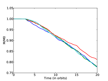
Figure 1: Time evolution of the total relative mass in the box when the number of cells in the vertical direction is varied: $N_{z}=256$ (blue line), $N_{z}=512$ (green line), $N_{z}=1024$ (red line) and $N_{z}=2048$ (light blue line). All other run parameters are fixed.

A peculiar aspect of SI09 is the low resolution they used, as noted by Guan & Gammie (2011). Indeed, the most unstable MRI mode has a vertical wave number given by $k_{z}v_{Az}\sim\Omega$ in an unstratified box. For $\beta=10^{4}$, as considered in the present paper and by SI09, this corresponds to a wavelength of about one tenth of the disk scale height. This wavelength is not adequately resolved in model ST09a in which we use $32$ cells per $H$. In stratified disks, the eigenmode structure is more complex and cannot be reduced to a single wave number, but Latter et al. (2010) have shown that about $200$ cells per scale height are required in this case to properly resolve the fastest growing eigenmode across the whole disk. In order to assess the importance of the vertical resolution on the existence and strength of the outflows that develop in model ST09a, we computed four models (Ideal256 to Ideal2048), gradually increasing the vertical resolution from $N_{z}=256$ to $N_{z}=2048$ while keeping all other parameters fixed. In figure 1, we plot the time-evolution of the total gas mass $M$ in the computational box, normalized by its initial value $M_{0}$. We find it is similar in the four models, regardless of the number of vertical cells. The values of $\dot{m}_{w}$ for the four models are reported in Table 1. They confirm the results of figure 1, as all values agree within $\pm 15\%$, with most of this scatter being due to model Ideal1024 for which we obtained a smaller mass loss rate than the other models. As a matter of fact, there is no systematic trend in the evolution of $\dot{m}_{w}$ with resolution. We conclude that there is only a modest effect of resolution, if any, on the result. It is tempting to associate this weak dependence with the morphology of the eigenmodes coupled with the fact that disk outflows are launched at $z\sim\pm 2H$, as SI09 and SMI10 do. Indeed, MRI modes have a shorter wavelength near the midplane and a longer wavelength at greater height (Latter et al. 2010). Since outflow rates are not set by conditions at the midplane, the mode structure at the midplane may be underresolved with little impact. Extending the classical result of Goodman & Xu (1994) to stratified boxes, Latter et al. (2010) have also shown that those modes are not only solution of the linear equation, but also nonlinear solutions in the limit of large $\beta$, such that some of their properties might affect the nonlinear flow dynamics. This reasoning would also agree with the claim of SI09 that such disk outflows are due to the breakup of channel modes in the disk corona. It is indeed likely that such channel modes will help the build up of strong fields in the disk atmosphere as is observed during the linear stage of the MRI. That having being said, the dynamics of the disk atmosphere during the remainder of the simulations is highly nonlinear and fluctuating. It might share some properties of the dynamics of channel modes, but a direct relationship between such outflows and linear MRI modes remains difficult to assess with certainty.

3.3 Explicit dissipation coefficients

The previous section has established that the mass outflow rate present a modest but apparently non–monotonic dependence with grid resolution. In addition, such simulations rely on grid resolution in order to stabilize the numerical scheme, the form and effects of which are more difficult to quantify than those of explicit dissipation. As explained in the introduction, it is also well known that the saturation properties of the turbulence depend strongly on the dissipation coefficients (Lesur & Longaretti 2007; Longaretti & Lesur 2010; Fromang et al. 2007; Fromang 2010; Simon & Hawley 2009; Davis et al. 2010; Simon et al. 2011b), regardless of the magnetic field configuration.

All these reasons argue in favor of including explicit dissipation in such simulations. Their introduction also makes the problem mathematically well posed. In contrast to the low-vertical-resolution simulations described above (for which numerical dissipation influences the linear phase of the instability), when viscosity and Ohmic resistivity are included the calculated growth rates and morphology of all the active MRI normal modes can be accurately reproduced in the simulations, providing a valuable code test. In the appendix, we describe the calculation of these modes as a function of $Re$ and $Rm$, extending the method used by Latter et al. (2010) in the ideal MHD limit. As shown in fig. 15, the linear modes display large-scale oscillations at $z\sim\pm 3H$ regardless of $Re$ and $Rm$, while the small-scale oscillations near the midplane are very much influenced by the magnitude of the dissipation coefficients. This structure could also explain the relative independence of the flow structure on resolution described in section 3.2.

One obvious limitation associated with explicit dissipation coefficients, though, is the tremendous computational costs associated with the grid resolution that is required for the dissipative lengthscales to be properly resolved. To keep the resolution requirements reasonable, we adopt in the remainder of this paper rather modest values for the dissipation coefficients such that $Re=3000$ for all simulations. We consider two values for $Rm$, namely $Rm=3000$ in our fiducial model and $Rm=1500$ in section 4.2. Past experience gained from unstratified simulations (see for example Fromang et al. 2007) suggests that $64$ cells per disk scale height are sufficient to capture correctly the flow properties at all relevant scales. The vertical profile of the eigenmode in such a case is illustrated in the bottom panel of fig. 15. Small scale oscillations near the midplane are damped by the large viscosity and resistivity. As a result, the most unstable eigenmode is easily captured even with such a modest resolution. This is another benefit gained from introducing dissipation in the problem. Before moving to a systematic study of the flow in such a viscous and resistive model, we briefly compare the outflow rate obtained in one such case (which we label model Diffu1H for future reference) with the cases without explicit dissipation described above, all other parameters being unchanged. As shown in Table 1, $\dot{m}_{w}$ is similar in all cases, regardless of the nature of the dissipation. This is in agreement with the above result that mass outflow rates are independent of the resolution, when explicit dissipation is absent. We will therefore adopt the setup of model Diffu1H as our fiducial model in the following and we now move to an extensive study of the disk outflow properties and saturation level of the turbulence using these parameters.

3.4 Influence of box size

3.4.1 Radial box size

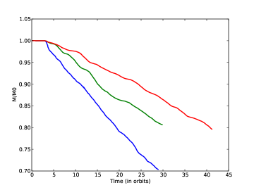
Figure 2: Time-evolution of the total relative mass in the box when the radial extent of the box is varied from $L_{x}=H$ (blue line) to $L_{x}=2H$ (green line) and $L_{x}=4H$ (red line).

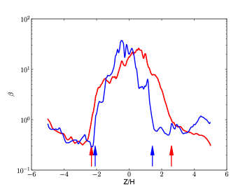
Figure 3: Vertical profile of the ratio $\beta$ between the horizontally averaged thermal pressure and the horizontally averaged magnetic pressure. The blue curve corresponds to model Diffu1H and results from a further time average between $t=10$ and $t=15$ orbits. The red curve was obtained averaging the data of model Diffu4H between $t=10$ and $t=30$. For each model, the vertical arrows report the approximate wind launching location where $\beta=1$ (SI09).

In a suite of numerical simulations of unstratified shearing boxes threaded by a net vertical flux, Bodo et al. (2008) discovered that the radial extension of the domain can significantly affect the properties of the turbulence. They demonstrated that channel flows develop in boxes of unit radial extent ($L_{x}=H$) while their influence is reduced in boxes having larger $L_{x}$. Since SI09 argue that the breakup of these channel flows drives structured disk winds, it is natural to ask whether the radial extent of the shearing box affects the disk outflow properties described above. This is the purpose of the present section.

To do so, we performed a series of simulations, successively doubling the radial extent of the box from $L_{x}=1H$ (model Diffu1H) to $L_{x}=4H$ (model Diffu4H). For each model, the time-evolution of the total mass inside the computational domain is shown in figure 2. The mass-loss rate gradually decreases as $L_{x}$ is increased. This is confirmed by Table 1, where $\dot{m}_{w}$ is found to be reduced by a factor of $2$ in the largest model. Such a lower mass-loss rate, apart from changing the properties of the outflow itself, also allows the simulation to be run for longer (and more statistics of the turbulence to be accumulated) before the reduction of the disk surface density starts affecting the disk structure. This is the reason why we could run model Diffu4H for $40$ orbits. A model with $L_{x}=8H$ (model Diffu8H) was also run and suggested numerical convergence for larger radial extent. However, its large resolution, $(N_{x},N_{y},N_{z})=(512,256,640)$, resulted in huge computational requirements that prevented the simulation from being run for more than 10 orbits. Clearly, this question needs further investigation but our preliminary result is not in disagreement with the conclusions of Bodo et al. (2008), who find good agreement between their $L_{x}=4$ and $L_{x}=8$ runs.

For a better understanding of the differences between these simulations, we turn to an examination of the wind launching location. SI09 have shown that this position can be evaluated to a good approximation by computing the location where the ratio $\beta$ between the horizontally averaged thermal pressure and the horizontally averaged magnetic pressure falls below unity. The vertical profile of $\beta$ is plotted in figure 3 for models Diffu1H and Diffu4H. For both models, $\beta$ is large in the turbulent midplane and decreases upwards. The location $z_{w}$ where it falls below unity is reported using vertical arrows. For the smallest radial box size, we measured $z_{w}=-2.1H$ and $2.3H$ respectively below and above the equatorial plane. The same values are $z_{w}=-2.7H$ and $2.9H$ when $L_{x}=4H$. Thus, in bigger boxes, disk outflows are launched at higher altitude, where the gas density is smaller, resulting in a smaller mass-loss rates. Ultimately, the higher location of the launching region can be be traced back to the toroidal magnetic field being weaker in the disk upper layers ($z\sim 2-3H$) in bigger boxes by a factor of about two, while the gas density varies by only a few percent at those locations. The physical mechanism responsible for this reduction of the toroidal magnetic field is uncertain, but could be due to the weakening of coherent structures as demonstrated by Bodo et al. (2008) in unstratified boxes. This weakening indeed results in more disordered magnetic fields (seen in the simulation as a larger ratio between the fluctuating and means parts of the azimuthal magnetic field) that reduce the efficiency with which outflows are accelerated.

3.4.2 Vertical box size

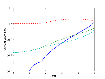
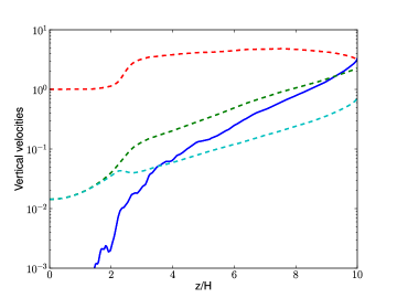
Figure 4: Vertical profiles of the vertical fluid and wave velocities. Horizontally and time-averaged fluid velocity $v_{z}$ (blue curve), slow magnetosonic speed $v_{sz}$ (light blue dashed curve), Alfvén speed $v_{Az}$ (green dashed curve) and fast magnetosonic speed $v_{fz}$ (red dashed curve), in units of $c_{0}$. The top panel shows results obtained in model Diffu4H ($L_{x}=4H$, $L_{z}=10H$) while the bottom panel is for the model Tall4H ($L_{x}=4H$, $L_{z}=20H$).

In numerical simulations, it is desirable for the outflow velocity to exceed all wave velocities before leaving the computational domain. When this occurs, no signal can propagate downwind, which guarantees that the results are independent of the box size and the boundary conditions. In the case of the magnetized outflows studied here, the relevant wave velocities are those of the Alfvén wave and the slow and fast magnetosonic waves, each of which gives rise to a critical point in the flow (Spruit 1996). Given the complexity of the flow, we will not consider wave velocities parallel to the fluid streamlines in this paper, but rather will focus on vertical velocity and wave velocities relative to the fluid. In the published simulations of SI09 and SMI10, no information is given as to whether the critical points are crossed, but this is probably not the case, because the flow velocity remains subsonic in some of the cases they report (see for example figure 3 of SI09).

In the present section, we investigate this issue by comparing the results of model Diffu4H, described above, with those of model Tall4H. The latter differs from the former only in its vertical extent, namely $L_{z}=20H$. We emphasize that the resolution of that simulation is large: $(N_{x},N_{y},N_{z})=(256,128,1280)$, which amounts to 40 million cells. Thus the computational requirements are significant and that model was evolved for only $20$ orbits. This is however sufficient to derive a reliable estimate of the mass-loss rate, as shown by both figures 1 and 2 for the models we have described so far. We found that the mass outflow is significantly reduced when doubling the vertical extent of the box. Indeed, table 1 shows that $\dot{m}_{w}$ is reduced by a factor of $3.4$. This is not a consequence of the mass flux steadily decreasing with $z$, as we observe in all simulations a constant $\langle\rho v_{z}\rangle$ above $z\sim 3H$, as reported also by Bai & Stone (2012). On the other hand, the existence of vertical boundaries could be preventing inflowing velocities. Indeed, both the 10H and 20H simulations display comparable outflowing mass fluxes at $z\pm 5H$, when only accounting for gas moving away from the midplane. This suggests that boxes with smaller vertical extents could lose material that would otherwise fall back on to the disk, thus artificially enhancing $\langle\rho v_{z}\rangle$. However this effect is absent by construction in the $1D$ simulations performed by Lesur et al. (2012) where the same dependence with vertical box size is obtained, thus questionning such an interpretation for the origin of the decrease.

Here, we consider an alternative explanation by investigating the location of the outflow critical points. In figure 4, the vertical profile of the vertical velocity (normalized by the sound speed) is compared with the vertical profile of the vertically propagating wave velocities (also normalized by $c_{0}$) for models Diffu4H (top panel) and Tall4H (bottom panel). The latter are given by the solutions of the following expression (Ogilvie 2012):

$$\left[v^{2}-v_{az}^{2}\right]\left[v^{4}-(c_{0}^{2}+v_{a}^{2})v^{2}+c_{0}^{2}v_{az}^{2}\right]=0\,,$$ (5)

where $\mbox{\boldmath{$v_{a}$}}=\mbox{\boldmath{$B$}}/\sqrt{\rho}$ is the Alfven velocity. Two comments can be made. In both panels, it is seen that only the slow and Alfvén points are crossed, while the fast magnetosonic point is, suspiciously, reached at the vertical boundary itself. The fact that this is the case in both models suggest that this is no coincidence, but is rather a numerical artifact probably associated with the shearing-box model or simply with the limited vertical extent of the computational domain. We note that such a failure to cross the fast magnetosonic point is not unlike published simulations of magnetically driven jets (Casse & Ferreira 2000, see their fig. 1) and has also recently been reported by Lesur et al. (2012) and Bai & Stone (2012) in simulations using a similar setup but performed with a different code. A second remark is that the slow and Alfvén points lie systematically higher up in the disk atmosphere in the taller model. The non-convergence of the location of those points might explain the different mass outflow rates measured in the two simulations (Spruit 1996).

We conclude this section by stressing the importance of this effect. The sensitivity to box size we obtain means that while $20\%$ of the mass in the box is lost within $20$ orbital times in the simulations of SI09, it would take about $140$ orbits to lose the same amount of mass in model Tall4H. The consequences for disk evolution would surely be significant.

4 Flow properties

As shown in both sections 3.4.1 and 3.4.2, it appears that many details of the computational setup affect the properties of outflows from MHD turbulent disks. The disappointing but unavoidable conclusion from these results is that the disk mass-loss rate due to such outflows cannot be robustly inferred in the framework of the shearing-box model. Nevertheless, we found that a number of properties of the flow are displayed by all simulations. The purpose of the present section is to describe these features and to analyse quantitatively the angular momentum transport associated with the turbulence.

However, one should be cautious when doing so. As already mentioned, the strong mass loss due to the outflow changes the disk structure itself on timescales of a few tens of orbits. For example, in model Diffu1H, we discovered that a strong mean toroidal field, with a strength close to equipartition, emerged in the disk midplane after $30$ orbits, perturbing its structure thereafter. No such perturbation was evident in model Diffu4H. In fact, all the diagnostics we considered suggest the disk is in a quasi-steady state during the first $20$ to $25$ orbits that follow the establishment of fully developed turbulence. This is why we will restrict our analysis in this section to the model having $L_{x}=4H$. Unless otherwise specified, time averages of the data will cover the range $5<t<30$.

4.1 Disk atmosphere: outflow structure

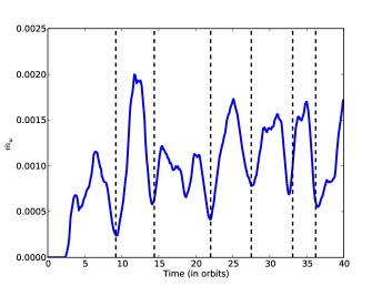
Figure 5: Time evolution of $\dot{m}_{w}$ for model Diffu4H (blue curve). The vertical lines mark the times at which the mean toroidal magnetic field at the top boundary of the box changes sign.

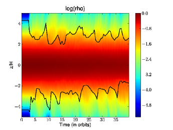
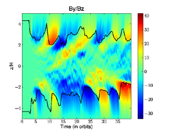
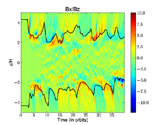
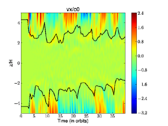
Figure 6: Space-time diagram of the logarithm of the horizontally averaged mass density (upper left panel), $\langle B_{y}\rangle/\langle B_{z}\rangle$ (upper right panel), $\langle B_{x}\rangle/\langle B_{z}\rangle$ (lower left panel) and $\langle v_{x}\rangle/c_{0}$ (lower right panel) for model Diffu4H. For all panels, the solid line shows the location of unit ratio of horizontally averaged thermal and magnetic pressures, $\beta=1$.

We first illustrate the flow structure with the help of figure 5 and 6. The first figure represents the time evolution of the mass loss rate $\dot{m}_{w}$. On the second figure, four space-time diagrams are plotted, representing the time-evolution of the vertical profiles of various horizontally averaged quantities. In addition, the location of unit ratio of the horizontally averaged thermal and magnetic pressures, $\beta=1$, is overplotted on each panel with a solid black line.

Several comments can be made based on these plots. First, the bursty nature of the outflows is illustrated by figure 5: $\dot{m}_{w}$ displays quasi–periodic variations during which the outflow rate increases by a factor of about $2$ to $3$. The typical duration of these bursts is seen to be roughly $5$ orbits. In addition figure 6 shows that these bursts are associated with higher density in the disk atmosphere and non-vanishing mean magnetic fields and radial velocity. The fact that launching occurs approximately at the location where $\beta=1$ is obvious from all the panels. The toroidal component of the horizontally averaged magnetic field $\langle B_{y}\rangle$ displays a cyclical behaviour above and below the midplane, akin to the ‘butterfly diagram’ reported by various authors (Gressel 2010; Shi et al. 2010; Davis et al. 2010; Simon et al. 2011b) for stratified zero-net-flux simulations. However, in contrast to the zero-net-flux situation where the mean toroidal flux arises from the disk midplane, it is seen here to originate at $z\sim 2$–$3H$, in agreement with the results reported by SI09. As shown by figure5, $\dot{m}_{w}$ is minimal when $\langle B_{y}\rangle$ changes sign, suggesting that the mean magnetic field is involved in the launching mechanism.

In the lower left and right panels, we plot the horizontally averaged radial components of the magnetic field $\langle B_{x}\rangle$ (normalized by $\langle B_{z}\rangle$) and velocity $\langle v_{x}\rangle$ (normalized by the sound speed $c_{0}$) are respectively shown (Note that, because of magnetic flux conservation, $\langle B_{z}\rangle$, which is used to normalize $\langle B_{y}\rangle$ in the upper right panel, is independent of $z$ and $t$ and equal to its initial value $B_{0}$). They show that a significant mean radial magnetic field and mean radial velocity develop in the disk atmosphere. Their amplitudes are comparable to those of $\langle B_{z}\rangle$ and $\langle v_{z}\rangle$, which means that both the poloidal magnetic field lines and the poloidal streamlines are significantly inclined with respect to the vertical axis. As expected because of the shear, the radial and toroidal components of the magnetic field are anti-correlated. Positive $\langle B_{y}\rangle$ corresponds to negative $\langle B_{x}\rangle$ and vice versa. The radial velocity also correlates positively with the radial magnetic field above the midplane (i.e. positive $\langle v_{x}\rangle$ corresponds to positive $\langle B_{x}\rangle$) but correlates negatively with it below the midplane (where positive $\langle v_{x}\rangle$ corresponds to negative $\langle B_{x}\rangle$). This flow morphology closely resembles that of the classical wind solution described by Blandford & Payne (1982, hereafter BP82). There are differences, though. First, in contrast to the steady-state BP82 solutions, the flow is strongly time-dependent here. Second, because of the symmetries associated with the shearing-box model, outflows are associated with poloidal magnetic field lines inclined towards either positive or negative $x$. This is different from the situation usually considered in cylindrical geometry in which magnetic field lines are inclined away from the central object in order to produce a successful outflow. As noted by Ogilvie (2012), the shearing box is unaware whether the central object is located in the direction of positive or negative $x$, and the local physics of wind launching is symmetrical. In our shearing-box simulations, there can even be situations where the poloidal field lines are directed towards positive $x$ above the disk midplane, but towards negative $x$ below the midplane (see, for example, the structure of the flow for $15<t<20$ in figure 6). Such unfamiliar flow morphologies are however permitted solutions of the equations in the framework of the shearing-box model (Ogilvie 2012; Lesur et al. 2012), and suggest that the outflows above and below the midplane are to some extent independent of each other.

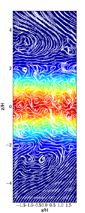
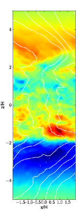
Figure 7: $y$–averaged poloidal streamlines (left panel) and poloidal magnetic field lines (right panel) in the $(x,z)$ plane, time–averaged over the ejection event occurring at $22<t<27$, and overplotted on the density distribution (left panel) and azimuthal magnetic field distribution (right panel).

Because of this variety of field configurations, and since the flow is not in steady state, it is not straightforward to illustrate the analogy with the BP82 solutions more quantitatively. In attempting to do so, we have isolated a single burst event that happens between the times $t=22$ and $t=27$ and have analysed it in more detail. Time-averaging the simulation data over such a short interval obviously means that the resulting curves will be noisy, but this is the price to be paid for a quantitative comparison with the theoretical expectations. The structure of the time–averaged flow is illustrated in figure 7. Poloidal streamlines and magnetic field lines, spatially averaged in the $y$ direction and time–averaged over the ejection event, are represented in the $(x,z)$ plane. They are overplotted on the density and azimuthal magnetic field distribution respectively. Poloidal magnetic field lines are systematically bent towards negative $x$ for $z\geq 3H$ and poloidal streamlines tend to align with those magnetic field lines, in a way that resembles Blandford & Payne type of solutions. In addition, a layer with a strong $B_{y}$ is apparent at the base the launching region, again consistent with this picture. In the following, we analysed quantitatively the properties of that flow.

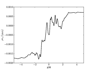
Figure 8: Vertical profile of the horizontally averaged vertical mass flux, $\langle\rho v_{z}\rangle$, obtained in model Diffu4H. The data are time-averaged over a single burst between $t=22$ and $t=27$ and normalized by $\rho_{0}c_{0}$.

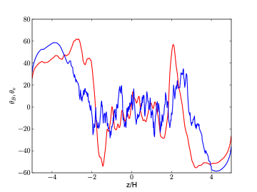
Figure 9: Vertical profiles of the angles $\theta_{B}$ (red curve) and $\theta_{v}$ (blue curve), measured between the vertical axis and the horizontally averaged poloidal magnetic and velocity fields, respectively. Both curves are obtained from model Diffu4H and are time-averaged over a single burst of ejection between $t=22$ and $t=27$.

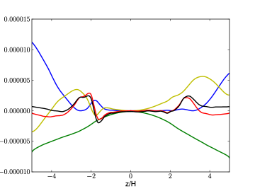
Figure 10: Vertical profiles of the quantities $E_{K}$ (blue curve), $E_{B}$ (red curve), $E_{T}$ (green curve), $E_{\phi}$ (yellow curve) and their sum $E$ (black) along a particular magnetic field line. Data have been horizontally averaged and time averaged between $t=22$ and $t=27$, i.e. over a single ejection event.

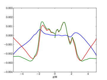
Figure 11: Vertical profiles of the quantities $\mathcal{L}$ (blue curve), $\langle B_{y}\rangle/\alpha$ (red curve) and the expected invariant $f=\mathcal{L}-\langle B_{y}\rangle/\alpha$ (green curve) along a particular magnetic field line, computed as in figure 10.

The first diagnostic we obtained is provided by the vertical mass flux. Its vertical profile is shown in figure 8. While small and fluctuating in the bulk of the disk, $\langle\rho v_{z}\rangle$ reaches a constant value for $|z/H|\geq 3$. This means the flow has reached a steady state in the disk atmosphere, and we can write

$$\langle\rho v_{z}\rangle=\alpha\langle B_{z}\rangle\,,$$ (6)

where $\alpha$ is constant beyond $|z|\sim 3H$. Under such conditions, it is well known that the flow is characterized by a number of features and invariants first studied in global models of disk winds (BP82; Pelletier & Pudritz 1992) and recently extended to the case of the shearing box (Lesur et al. 2012). First, poloidal streamlines approximately align with poloidal magnetic field lines, as shown on figure 7. In figure 9, we plot the vertical profiles of $\theta_{B}$ and $\theta_{v}$, which respectively denote the angles between the vertical axis and the horizontally averaged poloidal magnetic and velocity fields. In those regions where the vertical mass flux is constant, both $\theta_{B}$ and $\theta_{v}$ reach significant and fairly $z$-independent values of order $60^{\circ}$. These angles are comparable with each other ($\theta_{B}\sim\theta_{v}$) and larger than $30^{\circ}$, which is the critical angle in the BP82 analysis. This supports the BP82 scenario: poloidal streamlines are approximately aligned with poloidal magnetic fields and magneto-centrifugal launching is possible. Investigating whether this is actually the case can be examined using the Bernoulli invariant, which should be constant along magnetic field lines (Lesur et al. 2012):

$$E_{Ber} = E_{K}+E_{T}+E_{\phi}+E_{B}$$ (7)

$$= \frac{\langle v\rangle^{2}}{2}+c_{0}^{2}\log(\langle\rho\rangle)+\phi-\frac{\langle B_{y}\rangle v_{y}^{\star}}{\alpha}\,,$$

where $v_{y}^{\star}=\langle v_{y}\rangle-\alpha\langle B_{y}\rangle/\rho$ and $\phi$ represents the shearing box tidal potential. The variations of the four components of $E_{Ber}$ along a particular field line originating at the disk midplane are plotted in figure 10. Their sum is also represented using a black line, and exhibits a relatively flat profile beyond $|z|\sim 3H$, consistent with the expectations of steady state theory. Acceleration of the outflow, as seen by an increase of kinetic energy, occurs after the flow has reached a maximum in the potential energy. Its acceleration is essentially a result of a decrease of the potential energy along the field line. This demonstrates that the outflows are centrifugally driven, as observed for global simulations of laminar resistive disks. Note also that the variations of the thermal energy $E_{T}$ contribute to about one third of that acceleration, indicating a non–negligible effect of thermal pressure even above the Alfven point. This importance of thermal pressure is due to the plasma $\beta$ being much larger in the disk atmosphere (it is of order $1$) than is common in standard studies of outflow launching (where usually $\beta\ll 1$ in the launching region).

It is well known that such disk outflows carry angular momentum away from the disk midplane: angular momentum is extracted from the disk by the magnetic field before being transferred to gas as it is accelerated (Lesur et al. 2012). This exchange is described by the following invariant that should be constant on streamlines:

$$f=\mathcal{L}-\frac{\langle B_{y}\rangle}{\alpha},$$ (8)

where $\mathcal{L}=\langle v_{y}\rangle+(2-q)\Omega x$ plays the role of specific angular momentum in the shearing-box approximation. Its vertical profile along a particular streamline is plotted in figure 11. Its components $\mathcal{L}$ and $\langle B_{y}\rangle/\alpha$ are also represented for comparison. Beyond $|z|=3H$, $f$ shows a flat profile, with weak variations that are much smaller than the variations of its constituents. This is again consistent with the expectations of BP82: disk outflows extract angular momentum from the disk. As shown by Lesur et al. (2012), this leads to radial advection of gas and poloidal magnetic field lines. However, we failed to detect such an advection velocity. Averaging the radial mass flux over the single burst, we found

$$v_{x}^{*}=\frac{\int\int\langle\rho v_{x}\rangle dtdz}{\int\int\langle\rho\rangle dtdz}=2\times 10^{-3}c_{0}$$ (9)

This value is much below the turbulent velocity fluctuations, for which the Mach number is at the $10\%$ level. This suggest that outflow-mediated angular momentum transport is very small, as expected given the large value of $\beta_{0}$ we use, and consistent with the low altitude of the Alfvén point. We shall return into this issue in the discussion. We note also that even if the radial mass flux associated with these bursts appears to be small, it might still be locally important and influence the radial transport of vertical magnetic flux, as suggested by Spruit & Uzdensky (2005).

While enlightening as to the structure of the flow in the disk atmosphere, the above analysis should not hide the fact that the outflows that develop in the simulations are not strictly speaking BP82-type disk winds. First, one should not forget the non-steady nature of the flow, the properties of which are yet to be understood. How much of that variability is an artifact of the shearing-box symmetries should be investigated further. Another important difference with classical disk wind theories is that the outflows presented here do not pass all the relevant critical points within the computational domain. It is unlikely that the successful complete ejection of the outflow can be demonstrated within the local shearing-box model because the depth of the gravitational potential is not represented. We shall return to that point in the discussion (section 5.3). To summarize, even if the comparison drawn above is appealing, outflows driven by turbulent disks are clearly more complex than described by simple steady-state disk wind models. Working out simple models that will simultaneously describe the midplane turbulent flow and the non-steady BP82-like winds are beyond the scope of this paper and will surely prove challenging in the future.

4.2 Disk midplane: turbulent transport

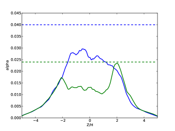
Figure 12: Vertical profile of the total stress tensor, normalized by the midplane pressure, for models Diffu4H (blue line) and Diffu4HPmhalf (green line). The blue and green dashed lines represent the corresponding values obtained in unstratified runs having the same parameters.

In this section, we focus on angular momentum transport. As argued above (see also section 5.2), it is likely dominated by turbulent transport occurring in the bulk of the disk. Here, we thus present a preliminary study of the saturation properties of the turbulence in stratified shearing boxes threaded by a mean magnetic field. In addition, we compare our results with identical simulations performed in the unstratified limit in order to assess the effect of density stratification on transport properties. Given the large computational expense associated with such a survey, we defer a systematic study of the scaling with vertical field amplitude to a future publication and consider here only the effect of the dissipation coefficients. To do so, we consider two models, the parameters of which are respectively $Re=Rm=3000$ (model Diffu4H) and $(Re,Rm)=(3000,1500)$ (model Diffu4Ha). Thus $Pm=1$ in the former and $0.5$ in the latter.

The $xy$-component of the sum of the Reynolds and Maxwell stresses, normalized by the midplane pressure, can be taken to define a local value for the Shakura–Sunyaev $\alpha_{SS}$ viscosity parameter. Its vertical profile is plotted in figure 12 for both models. As reported in the literature for different configurations, turbulent transport increases with $Pm$. We found the vertically averaged value to be $\alpha_{SS}=6.2\times 10^{-2}$ when $Pm=1$ and $\alpha_{SS}=4.8\times 10^{-2}$ when $Pm=0.5$. The vertical profile of the stress we obtained in each case is comparable to that reported in the literature by many authors using local or global simulations (Miller & Stone 2000; Hirose et al. 2006; Fromang & Nelson 2006; Flaig et al. 2010; Dzyurkevich et al. 2010; Sorathia et al. 2010; Fromang et al. 2011; Simon et al. 2011b). It is rather flat in the bulk of the disk, with possible local maxima at $z\sim 2H$ before dropping to low values in the corona. Theoretical arguments tentatively explaining such a profile have also recently been proposed in the literature (Guan & Gammie 2011; Uzdensky 2012). The reason why the local maxima are more apparent in the lower $Pm$ case is unclear and deserve future investigations, but might be related to the different turbulent states described by Simon et al. (2011b) for vanishing vertical flux configurations or simply to the resistivity being larger in the case $Pm=0.5$. As shown by the dashed lines in figure 12, the transport rates we measured are in acceptable agreement with results obtained in unstratified boxes. In such cases, we indeed obtained $\alpha_{SS}=4.0\times 10^{-2}$ and $2.4\times 10^{-2}$ when $Pm=1$ and $0.5$, respectively. These values are higher by about a factor of two than the midplane value of the transport rates obtained in the stratified models and display the same trend with magnetic Prandtl number. This means that unstratified shearing-box simulations with net flux, such as reported by Longaretti & Lesur (2010), provide a good first-order estimate of angular momentum transport in stratified disks.

5 Discussion

In this section, we discuss several controversial aspects of the present simulations, namely the influence of vertical boundary conditions on our results, the relative importance of turbulent and outflow-mediated angular momentum transport, and possible issues associated with a straightforward truncation of the shearing-box vertical potential.

5.1 Influence of the vertical boundary conditions

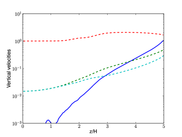
Figure 13: Same as figure 4, but for the model having zero-gradient vertical boundary conditions on $B_{x}$ and $B_{y}$.

Clearly, it is not satisfying to see such a strong dependence of the outflow mass-loss rate on numerical aspects of the setup. One might worry that some of this dependence is due to the vertical boundary conditions. In particular, our choice of purely vertical magnetic fields at the top and bottom of the computational box is rather unfortunate. Indeed, it does not favour magneto-centrifugal acceleration as the latter requires magnetic field lines inclined by more than $30^{\circ}$ to operate. This might affect the flow and prevent successful launching of disk outflows.

In order to test that possibility, we performed an additional simulation with different boundary conditions on the magnetic field. We adopted zero-gradient boundary conditions for $B_{x}$ and $B_{y}$ at the top and bottom of the box. To save computational power, this simulation was performed without explicit dissipation coefficients and with a smaller resolution of $32$ cells per $H$, using the same box size as for model Diffu4H, namely $(L_{x},L_{y},L_{z})=(4H,4H,10H)$. We obtained $\dot{m}_{w}=1.0\times 10^{-3}$. This is very similar to the mass outflow rates obtained for models Diffu4H and Diffu4Ha that share the same box size. As an additional check, we plot in figure 13 a comparison between the vertical gas velocity and the various wave velocities of the problem, as done for model Diffu4H in the top panel of figure 4. The two plots are very similar, indicating a weak effect of the boundary conditions on the flow properties (note, however that, as opposed to mode Diffu4H, the flow velocity remains smaller that the sound speed everywhere).

Thus, we have shown in this paper that our results are unchanged when we adopt widely used boundary conditions for the magnetic field (purely vertical field or zero gradient for its horizontal components). The good agreement with the results published by SI09 and SMI10 suggests that this insensitivity to vertical boundary conditions extends to more elaborate boundary conditions. This is strange as we have shown that the results depend on vertical box size (section 3.4.2) which indicates that the flow knows about the existence of an upper boundary. Its seems that the artifacts uncovered in the present paper are due to the very existence of a boundary rather that the nature of the conditions imposed there. Alternatively, this could indicate a breakdown of the shearing–box model itself. Future investigations along with comparison with global simulations are needed to clarify this issue.

5.2 Vertical vs. turbulent transport of angular momentum

The paradigm that emerges out of the analysis performed in this paper is that of a turbulent disk surrounded by transient and presumably local magneto-centrifugally accelerated BP82-like outflows. As demonstrated in figure 11, such outflows carry angular momentum away from the bulk of the disk, the amount of which might be important for its evolution. In this section, we speculate on the relative importance of the angular momentum transported vertically by the outflow and radially by the turbulence.

Given the symmetries of the shearing box, there is some ambiguity in determining that ratio. One possibility we explored is to separate the flow into mean fields and fluctuations and to assign the transport mediated by the former to the outflow and that due to the latter to the turbulence. However, we found significant radial transport due to the mean magnetic field, the role of which remains unclear. We therefore followed the approach sketched by Wardle (2007) for a radially structured accretion disk. In cylindrical coordinates $(R,\phi,Z)$, we first write the horizontal velocities $v_{R}$ and $v_{\phi}$ as the sum of an azimuthally averaged part and remaining fluctuations:

$$v_{R} = \langle v_{R}\rangle+\delta v_{R}\,,$$ (10)

$$v_{\phi} = \langle v_{\phi}\rangle+\delta v_{\phi}=R\Omega+\delta v_{\phi}\,.$$ (11)

Angular momentum conservation in a steady-state disk is then written

$$R\langle\rho v_{R}\rangle\frac{\partial R^{2}\Omega}{\partial R}=\frac{\partial}{\partial R}\left(R^{2}T_{R\phi}\right)+\frac{\partial}{\partial Z}\left(R^{2}T_{Z\phi}\right)\,,$$ (12)

with the turbulent stress tensors $T_{R\phi}$ and $T_{Z\phi}$ expressed as (Balbus & Papaloizou 1999):

$$T_{R\phi} = \langle B_{R}B_{\phi}-\rho\delta v_{R}\delta v_{\phi}\rangle$$ (13)

$$T_{Z\phi} = \langle B_{Z}B_{\phi}-\rho v_{Z}\delta v_{\phi}\rangle\,,$$ (14)

We now assume that there exist disk surfaces located at $Z=\pm Z_{s}(R)$ above and below which mass and angular momentum are outflowing. We define the mass accretion rate in the disk as

$$\dot{M}=-2\pi R\int_{-Z_{s}}^{+Z_{s}}\langle\rho v_{R}\rangle dZ$$ (15)

and integrate Eq. (12) between $-Z_{s}$ and $+Z_{s}$. We find

$$\frac{\dot{M}}{2\pi R}\frac{\partial R^{2}\Omega}{\partial R}=\dot{m}_{R}+\dot{m}_{Z}\,,$$ (16)

where $\dot{m}_{R}$ and $\dot{m}_{Z}$ respectively denote the disk and the outflow contribution to the angular momentum transport and are given by

$$\dot{m}_{R} = -\frac{1}{R}\frac{\partial}{\partial R}\left(R^{2}\int_{-Z_{s}}^{+Z_{s}}T_{R\phi}dZ\right)\,,$$ (17)

$$\dot{m}_{Z} = -R\left[T_{Z\phi}\right]_{-Z_{s}}^{+Z_{s}}\,.$$ (18)

The relative importance of turbulence and outflowing material to angular momentum transport is given by the ratio of $\dot{m}_{R}$ and $\dot{m}_{Z}$. In the shearing box, however, $\dot{m}_{R}$ artificially vanishes because of symmetries of the model. It is possible, though, to use the shearing box results to make such a evaluation for real disks, provided reasonable assumptions are made about the disk structure. Let us first assume that the vertical profile of the stress, when normalized by the midplane pressure $P_{mid}$, is a “universal” function of $\tilde{Z}=Z/H$ only, and is independent of $R$ (which amounts to saying that $\alpha$ is radially constant). Then all the radial dependence in $\dot{m}_{R}$ can be made explicit provided we give ourselves radial scalings for the surface density $\Sigma\propto R^{p}$ and the sound speed $c_{0}^{2}\propto R^{q}$ (we assume a locally isothermal equation of state, i.e. that $c_{0}$ a function of $R$ only, which means the vertical density profile is Gaussian). After some algebra, we obtain

$$\dot{m}_{R}=(p+q+2)\overline{\alpha_{R}}\frac{\Sigma c_{0}^{2}}{\sqrt{2\pi}},$$ (19)

where we have defined the radius-independent variable $\overline{\alpha_{R}}$ as

$$\overline{\alpha_{R}}=\int_{-\tilde{Z_{s}}}^{+\tilde{Z_{s}}}\alpha_{R}(\tilde{Z})d\tilde{Z}=-\int_{-\tilde{Z_{s}}}^{+\tilde{Z_{s}}}\frac{T_{R\phi}}{P_{mid}}d\tilde{Z},$$ (20)

and the second equality serves as a definition of $\alpha_{R}(\tilde{Z})$. The interest of the last pair of equations is that $\overline{\alpha_{R}}$ can be derived from shearing-box simulations such as presented in the present paper. Similarly, $\dot{m}_{Z}$ can be written as

$$\dot{m}_{Z}=\left(\frac{R}{H}\right)[\alpha_{Z}]_{-Z_{s}}^{+Z_{s}}\frac{\Sigma c_{0}^{2}}{\sqrt{2\pi}},$$ (21)

where $\alpha_{Z}=-T_{Z\phi}/P_{mid}$, so that the ratio $\dot{m}_{R}/\dot{m}_{Z}$ is given by

$$\frac{\dot{m}_{R}}{|\dot{m}_{Z}|}=(p+q+2)\left(\frac{H}{R}\right)\frac{\overline{\alpha_{R}}}{\left|[\alpha_{Z}]_{-Z_{s}}^{+Z_{s}}\right|}\,.$$ (22)

Note the absolute value in the expression above which accounts for the facts that outflow-mediated angular momentum transport can be directed either way in the shearing box. We are interested here only in its amplitude.

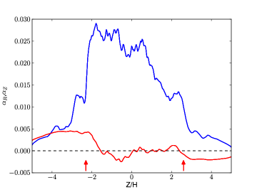
Figure 14: Vertical profile of $\alpha_{R}$ (blue curve) and $\alpha_{Z}$ (red curve), time averaged using the data of model Diffu4H over the interval $22<t<27$. Vertical arrows marks the location of unit ratio between horizontally averaged thermal and magnetic pressures.

Using model Diffu4H, we measured $\alpha_{R}$ and $\alpha_{Z}$. We focus on the same burst that we studied in section 4.1, and thus averaged the simulation data between $t=22$ and $t=27$. The vertical profiles we obtained by doing so are plotted in figure 14 along with vertical arrows showing the ejection region calculated as in fig. 3. At first glance, fig. 14 shows than $\alpha_{R}$ is larger than $\alpha_{Z}$. This is confirmed by precise measurements, which give $\overline{\alpha_{R}}=1.0\times 10^{-1}$ and $[\alpha_{Z}]_{-Z_{s}}^{+Z_{s}}=-4.4\times 10^{-3}$. Note that we have taken $Z_{s}=2.5H$ in making that estimate. Taking $p+q+2$ to be of order unity in Eq. (22), this gives

$$\frac{\dot{m}_{R}}{|\dot{m}_{Z}|}\sim 24\left(\frac{H}{R}\right)\,.$$ (23)

This means that turbulent transport dominates outflow-mediated transport as long as $H/R>0.04$. We stress, however, that outflows are more difficult to launch in thinner disks because the escape Mach number is larger in that case. Indeed, $v_{esc}=\sqrt{2}v_{\phi}$, which translates into $v_{esc}/c_{0}=\sqrt{2}(R/H)$. Thus, in thin disks where we can imagine outflow-mediated transport to dominate, its vertical Mach number should exceed $\sim 35$ for successful ejection. As demonstrated in both panels of figure 4, this is far from being the case in the simulations we have been able to run, in which the vertical Mach number reaches at most values of a few. Thus the question of whether such outflows will eventually escape the potential well or fall back on the disk is still an open issue.

Finally, we end this section by stressing that the nature of the transport in the disk corona is still uncertain. Although part of it should be attributed to the presence of the outflow, some of the radial transport could be due to coronal magnetic loops transmitting angular momentum between their footpoints as suggested by Uzdensky & Goodman (2008). Since the disk outflow also carries angular momentum radially in the shearing box model, it is difficult to disentangle the relative contribution of the two mechanisms.

5.3 Smoothing the shearing-box potential?

It is obvious that the shearing-box model suffers from a number of artifacts that might affect the results presented here. Maybe the most important of them is the singular nature of the tidal potential used in our simulations. In standard shearing-box simulations, the potential is given as

$$\phi_{sb}=-\frac{3}{2}\Omega^{2}x^{2}+\frac{1}{2}\Omega^{2}z^{2}\,.$$ (24)

The second term shows that the potential becomes deeper and deeper as the vertical box size is increased. This means it requires larger and larger energy for gas to climb out of that potential, while in reality the gravitational potential has a finite depth

$$\phi_{g}=-\frac{GM_{\star}}{\sqrt{R^{2}+Z^{2}}}\,.$$ (25)

The second term in Eq. (24) is simply the second-order Taylor expansion of the last equation with respect to $z$.

SMI10 investigated this issue by directly employing the potential given by Eq. (25). They obtain results that are difficult to interpret as $\dot{m}_{w}$ display variations by factors of $2$–$3$ and show no systematic trend with vertical box size. Here, we caution that a more rigorous and self–consistent approach is to include the next order in the expansion of the tidal potential. Up to the first terms that include a modification of its vertical profile, such an expansion is written

$$\phi=\phi_{sb}+\left(\frac{H}{R}\right)c_{0}^{2}\left[\tilde{x}^{3}-\frac{3}{2}\tilde{x}\tilde{z}^{2}\right]$$ (26)

where we have noted $\tilde{x}=x/H$ and $\tilde{z}=z/H$ and use the relation $H=c_{0}/\Omega$.

The expression above shows that the first additional terms in the expansion involves $x$ as well as $z$. This means that smoothing the potential should be done by simultaneously altering the radial component of the tidal force. We note that in such a situation, curvature terms should also be accounted for, and the shearing-periodic boundary conditions would be incompatible with the governing equations. The first nonzero term involving $z$ that appears in the potential expansion scales like $xz^{2}$. In practice, this term change the equilibrium shear itself, making it $z$–dependent. For a barotropic gas as considered here, this violates the results that rotation should be on cylinders (Tassoul 1978), unless the equilibrium profile of the density depends on $x$ as well as on $z$. This is a significant modification to the standard shearing box model. In practice, smoothing can only be achieved with higher order terms that are in $(H/R)^{2}$, among which a term in $-z^{4}$ that results in a finite potential barrier out of which to climb, albeit with an incorrect value. These complications were not addressed in the SMI10 analysis, which makes the interpretation of their results unclear.

Clearly, the discussion above shows that changing the vertical profile of the tidal potential is a risky avenue, much beyond the scope of this paper. It has to be done in a way that is consistent with all the approximations involved in the shearing box. The extension of the shearing-box model in that direction is promising for the analysis of outflow-related issues and should be the subject of future work.

6 Conclusions and perspectives

In this paper, we have analysed in detail the structure of the flow in an accretion disk threaded by a weak vertical magnetic field. In agreement with previous results (SI09, SMI10), we find that a strong outflow develops, with mass-loss rates that deplete the gas content of the computational box within a hundred dynamical times. However, we found these mass-loss rates to depend strongly on the numerical setup, thus preventing a reliable estimate of such outflow rates from being made in shearing-box simulations. Nevertheless, we found that the flow properties in the disk atmosphere exhibit robust features: outflows are magneto-centrifugally accelerated, yet thermal pressure has a non negligible effect. We recover the same invariants that characterized classical theories of steady-state disk winds (BP82; Pelletier & Pudritz 1992). We stress however, that there are a number of important differences with such theories: first, the outflows produced in the simulations are strongly time-dependent, which means steady state models should be used with care. Second, the vertical outflow velocity is never seen to exceed the fast magnetosonic speed. In addition, the positions of the slow magnetosonic point and the Alfvén point are seen to depend on box size. This highlights the fact that information can come back down the outflow, although we have not been able to find any significant modifications of its properties by changing the nature of the vertical boundary conditions. Finally, and maybe most importantly, we found that the dynamical effect of these outflows on accretion disks remains to be demonstrated: we investigated the ratio of the angular momentum extraction by such outflows and its radial transport by turbulence. These quantities might become comparable for thin disks for which the escape velocity is larger by more than one order of magnitude than the velocities observed in the simulations. Thus, the ultimate fate of these outflows, either successful launching or falling back onto the disk, remains unclear.

These results should be contrasted with a case of stronger, MRI stable magnetic field. In that situation, Ogilvie (2012) has argued, with reference to previous work, that the local approximation can be used to determine the mass-loss rate per unit area in magnetized outflows that are accelerated along inclined poloidal magnetic field lines (Blandford & Payne 1982). In turbulent disks as studied in the present paper, this result does not hold. The occurrence of transient, and presumably local, outflows appears to be a natural consequence of the nonlinear development of the MRI in a stratified disk in the presence of a net vertical magnetic field. This behaviour is different from that in incompressible disks, where no vertical motion arises from nonlinear channel modes because the vertical forces are cancelled by pressure gradients (Goodman & Xu 1994). Nevertheless, the connection between these transient and local outflows and the large-scale jets observed from astrophysical discs is still unclear. Traditional models for large-scale outflows have strong, ordered magnetic fields and Alfvén points high above the surface of the disk, rather different from the situation in our simulations.

In the light of our results, it appears that the shearing-box model is not well adapted to answer these questions, unless new developments are undertaken that go much beyond its original formulation. Both quantitative mass-loss rates and the ultimate fate of these outflows may have to be determined using global numerical simulations. This is a formidable task, the computational cost of which is at the limit of currently available facilities. But perhaps the good news of our work is that moderate resolution and runtime are sufficient to capture the properties of disk outflows. This gives hope that the questions of the fate, properties and consequences of outflows for accretion disk dynamics can be answered in the next few years.

Appendix A Linear modes in viscous and resistive stratified disks

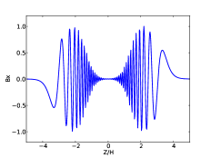
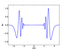
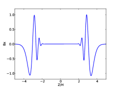
Figure 15: Vertical profile of the radial magnetic field eigenmode for three different sets of dissipation coefficients. From left to right, $Rm=Re=10^{6}$, $Rm=Re=10^{4}$ and $Rm=Re=3000$.

Consider an MRI channel flow of the following form:

$$\mbox{\boldmath{$u$}}^{\text{ch}}=H\Omega\,e^{st}\left[\mbox{\boldmath{$i$}}\,u_{x}(z)+\mbox{\boldmath{$k$}}\,u_{y}(z)\right],$$ (27)

$$\mbox{\boldmath{$B$}}^{\text{ch}}=B_{0}\,e^{st}\left[\mbox{\boldmath{$i$}}\,B_{x}(z)+\mbox{\boldmath{$k$}}\,B_{y}(z)\right],$$ (28)

where $H$ is the disk semithickness, $B_{0}$ is the amplitude of the background vertical field, $s$ is the growth rate, and $u_{x}$, $u_{y}$, $B_{x}$ and $B_{y}$ are dimensionless functions to be determined. Note that in the limit of high midplane $\beta$ (anelastic approximation) this flow is both a linear and nonlinear solution to the equations of non-ideal MHD in the vertically stratified shearing box (cf. Latter et al. 2010).

We denote the background density as $\rho=\rho_{0}\,h(z)$ where $h$ is a dimensionless function, and then scale time by $1/\Omega$ and space by $H$. The four equations to be solved are then

$$s\,u_{x} =2\,u_{y}+\frac{2}{\beta}\,\frac{1}{h}\,B_{x}^{\prime}+\frac{1}{Re}\frac{1}{h}\,(h\,u_{x}^{\prime})^{\prime},$$ (29)

$$s\,u_{y} =-\frac{1}{2}\,u_{x}+\frac{2}{\beta}\,\frac{1}{h}\,B_{y}^{\prime}+\frac{1}{Re}\frac{1}{h}\,(h\,u_{y}^{\prime})^{\prime},$$ (30)

$$s\,B_{x} =u_{x}^{\prime}+\frac{1}{Rm}\,B_{x}^{\prime\prime},$$ (31)

$$s\,B_{y} =u_{y}^{\prime}-\frac{3}{2}\,B_{x}+\frac{1}{Rm}B_{y}^{\prime\prime},$$ (32)

where a prime indicates differentiation with respect to $z$. This set of equations can be solved via a pseudo-spectral method using Whittaker cardinal functions, as outlined in Latter et al. (2010).

Examples of these calculations are plotted in Fig. 15. Note in these profiles how the combined action of magnetic diffusion and viscosity dramatically alters the mode morphology even for relatively large $Re$ and $Rm$. In the ideal case, the modes are concentrated near the miplane, where they also exhibit their shortest scales. These short scales, however, are vulnerable to even a small amount of dissipation, and when present the modes as a consequence tend to localise near $z=\pm 2$-$3H$ where their characteristic scale is longer.

References

- Bai & Stone (2012) Bai, X.-N. & Stone, J. M. 2012, ArXiv e-prints
- Balbus & Hawley (1991) Balbus, S. & Hawley, J. 1991, ApJ, 376, 214
- Balbus & Hawley (1998) Balbus, S. & Hawley, J. 1998, Rev.Mod.Phys., 70, 1
- Balbus & Papaloizou (1999) Balbus, S. & Papaloizou, J. 1999, ApJ, 521, 650
- Blandford & Payne (1982) Blandford, R. D. & Payne, D. G. 1982, MNRAS, 199, 883
- Bodo et al. (2011) Bodo, G., Cattaneo, F., Ferrari, A., Mignone, A., & Rossi, P. 2011, ApJ, 739, 82
- Bodo et al. (2008) Bodo, G., Mignone, A., Cattaneo, F., Rossi, P., & Ferrari, A. 2008, A&A, 487, 1
- Brandenburg et al. (1995) Brandenburg, A., Nordlund, A., Stein, R. F., & Torkelsson, U. 1995, ApJ, 446, 741
- Casse & Ferreira (2000) Casse, F. & Ferreira, J. 2000, A&A, 353, 1115
- Commerçon et al. (2010) Commerçon, B., Hennebelle, P., Audit, E., Chabrier, G., & Teyssier, R. 2010, A&A, 510, L3
- Dapp et al. (2012) Dapp, W. B., Basu, S., & Kunz, M. W. 2012, A&A, 541, A35
- Davis et al. (2010) Davis, S. W., Stone, J. M., & Pessah, M. E. 2010, ApJ, 713, 52
- Dzyurkevich et al. (2010) Dzyurkevich, N., Flock, M., Turner, N. J., Klahr, H., & Henning, T. 2010, A&A, 515, A70+
- Flaig et al. (2010) Flaig, M., Kley, W., & Kissmann, R. 2010, ArXiv e-prints
- Flaig et al. (2012) Flaig, M., Ruoff, P., Kley, W., & Kissmann, R. 2012, MNRAS, 420, 2419
- Fleming & Stone (2003) Fleming, T. & Stone, J. M. 2003, ApJ, 585, 908
- Fromang (2010) Fromang, S. 2010, A&A, 514, L5
- Fromang et al. (2006) Fromang, S., Hennebelle, P., & Teyssier, R. 2006, A&A, 457, 371
- Fromang et al. (2011) Fromang, S., Lyra, W., & Masset, F. 2011, A&A, 534, A107
- Fromang & Nelson (2006) Fromang, S. & Nelson, R. P. 2006, A&A, 457, 343
- Fromang et al. (2007) Fromang, S., Papaloizou, J., Lesur, G., & Heinemann, T. 2007, A&A, 476, 1123
- Fromang & Stone (2009) Fromang, S. & Stone, J. M. 2009, A&A, 507, 19
- Goldreich & Lynden-Bell (1965) Goldreich, P. & Lynden-Bell, D. 1965, MNRAS, 130, 125
- Goodman & Xu (1994) Goodman, J. & Xu, G. 1994, ApJ, 432, 213
- Gressel (2010) Gressel, O. 2010, MNRAS, 405, 41
- Gressel et al. (2011) Gressel, O., Nelson, R. P., & Turner, N. J. 2011, MNRAS, 415, 3291
- Guan & Gammie (2011) Guan, X. & Gammie, C. F. 2011, ApJ, 728, 130
- Hawley et al. (1995) Hawley, J. F., Gammie, C. F., & Balbus, S. A. 1995, ApJ, 440, 742
- Hennebelle & Ciardi (2009) Hennebelle, P. & Ciardi, A. 2009, A&A, 506, L29
- Hennebelle et al. (2011) Hennebelle, P., Commerçon, B., Joos, M., et al. 2011, A&A, 528, A72
- Hennebelle & Fromang (2008) Hennebelle, P. & Fromang, S. 2008, A&A, 477, 9
- Hirose et al. (2006) Hirose, S., Krolik, J. H., & Stone, J. M. 2006, ApJ, 640, 901
- Johansen & Levin (2008) Johansen, A. & Levin, Y. 2008, A&A, 490, 501
- Johnson et al. (2008) Johnson, B. M., Guan, X., & Gammie, C. F. 2008, ApJS, 177, 373
- Joos et al. (2012) Joos, M., Hennebelle, P., & Ciardi, A. 2012, ArXiv e-prints
- Krasnopolsky et al. (2010) Krasnopolsky, R., Li, Z.-Y., & Shang, H. 2010, ApJ, 716, 1541
- Krasnopolsky et al. (2011) Krasnopolsky, R., Li, Z.-Y., & Shang, H. 2011, ApJ, 733, 54
- Latter et al. (2010) Latter, H. N., Fromang, S., & Gressel, O. 2010, MNRAS, 406, 848
- Lesur et al. (2012) Lesur, G., Ferreira, J., & Ogilvie, G. I. 2012, submitted
- Lesur & Longaretti (2007) Lesur, G. & Longaretti, P.-Y. 2007, MNRAS, 378, 1471
- Li et al. (2011) Li, Z.-Y., Krasnopolsky, R., & Shang, H. 2011, ApJ, 738, 180
- Longaretti & Lesur (2010) Longaretti, P. & Lesur, G. 2010, A&A, submitted
- Masset (2000) Masset, F. 2000, A&AS, 141, 165
- Mellon & Li (2009) Mellon, R. R. & Li, Z.-Y. 2009, ApJ, 698, 922
- Miller & Stone (2000) Miller, K. A. & Stone, J. M. 2000, ApJ, 534, 398
- Miyoshi & Kusano (2005) Miyoshi, T. & Kusano, K. 2005, Journal of Computational Physics, 208, 315
- Moll (2012) Moll, R. 2012, ArXiv e-prints
- Ogilvie (2012) Ogilvie, G. I. 2012, MNRAS, 423, 1318
- Oishi & Mac Low (2009) Oishi, J. S. & Mac Low, M.-M. 2009, ApJ, 704, 1239
- Pelletier & Pudritz (1992) Pelletier, G. & Pudritz, R. E. 1992, ApJ, 394, 117
- Santos-Lima et al. (2012) Santos-Lima, R., de Gouveia Dal Pino, E. M., & Lazarian, A. 2012, ApJ, 747, 21
- Seifried et al. (2011) Seifried, D., Banerjee, R., Klessen, R. S., Duffin, D., & Pudritz, R. E. 2011, MNRAS, 417, 1054
- Shi et al. (2010) Shi, J., Krolik, J. H., & Hirose, S. 2010, ApJ, 708, 1716
- Simon et al. (2011a) Simon, J. B., Armitage, P. J., & Beckwith, K. 2011a, ApJ, 743, 17
- Simon & Hawley (2009) Simon, J. B. & Hawley, J. F. 2009, ApJ, 707, 833
- Simon et al. (2011b) Simon, J. B., Hawley, J. F., & Beckwith, K. 2011b, ApJ, 730, 94
- Sorathia et al. (2010) Sorathia, K. A., Reynolds, C. S., & Armitage, P. J. 2010, ApJ, 712, 1241
- Spruit (1996) Spruit, H. C. 1996, in NATO ASIC Proc. 477: Evolutionary Processes in Binary Stars, ed. R. A. M. J. Wijers, M. B. Davies, & C. A. Tout, 249–286
- Spruit & Uzdensky (2005) Spruit, H. C. & Uzdensky, D. A. 2005, ApJ, 629, 960
- Stone & Gardiner (2010) Stone, J. M. & Gardiner, T. A. 2010, ApJS, 189, 142
- Stone et al. (2008) Stone, J. M., Gardiner, T. A., Teuben, P., Hawley, J. F., & Simon, J. B. 2008, ApJS, 178, 137
- Stone et al. (1996) Stone, J. M., Hawley, J. F., Gammie, C. F., & Balbus, S. A. 1996, ApJ, 463, 656
- Suresh (2000) Suresh, A. 2000, SIAM J. Sci. Comp., 22, 1184
- Suzuki & Inutsuka (2006) Suzuki, T. K. & Inutsuka, S.-i. 2006, Journal of Geophysical Research (Space Physics), 111, 6101
- Suzuki & Inutsuka (2009) Suzuki, T. K. & Inutsuka, S.-i. 2009, ApJ, 691, L49
- Suzuki et al. (2010) Suzuki, T. K., Muto, T., & Inutsuka, S.-i. 2010, ApJ, 718, 1289
- Tassoul (1978) Tassoul, J. 1978, Theory of rotating stars (Princeton Series in Astrophysics, Princeton: University Press, 1978)
- Teyssier (2002) Teyssier, R. 2002, A&A, 385, 337
- Toro (1997) Toro, E. 1997, Riemann solvers and numerical methods for fluid dynamics (Springer)
- Turner et al. (2006) Turner, N. J., Willacy, K., Bryden, G., & Yorke, H. W. 2006, ApJ, 639, 1218
- Uzdensky (2012) Uzdensky, D. A. 2012, ArXiv e-prints
- Uzdensky & Goodman (2008) Uzdensky, D. A. & Goodman, J. 2008, ApJ, 682, 608
- Wardle (1997) Wardle, M. 1997, in Astronomical Society of the Pacific Conference Series, Vol. 121, IAU Colloq. 163: Accretion Phenomena and Related Outflows, ed. D. T. Wickramasinghe, G. V. Bicknell, & L. Ferrario, 561
- Wardle (2007) Wardle, M. 2007, Ap&SS, 311, 35
- Ziegler & Rüdiger (2000) Ziegler, U. & Rüdiger, G. 2000, A&A, 356, 1141