Local Study of Accretion Disks with a Strong Vertical Magnetic Field: Magnetorotational Instability and Disk Outflow

Abstract

We perform three-dimensional vertically-stratified local shearing-box ideal MHD simulations of the magnetorotational instability (MRI) that include a net vertical magnetic flux, which is characterized by midplane plasma $\beta_{0}$ (ratio of gas to magnetic pressure). We have considered $\beta_{0}=10^{2},10^{3}$ and $10^{4}$ and in the first two cases the most unstable linear MRI modes are well resolved in the simulations. We find that the behavior of the MRI turbulence strongly depends on $\beta_{0}$: The radial transport of angular momentum increases with net vertical flux, achieving $\alpha\sim 0.08$ for $\beta=10^{4}$ and $\alpha\gtrsim 1.0$ for $\beta_{0}=100$, where $\alpha$ is the height-integrated and mass-weighted Shakura-Sunyaev parameter. A critical value lies at $\beta_{0}\sim 10^{3}$: For $\beta_{0}\gtrsim 10^{3}$, the disk consists of a gas pressure dominated midplane and a magnetically dominated corona. The turbulent strength increases with net flux, and angular momentum transport is dominated by turbulent fluctuations. The magnetic dynamo that leads to cyclic flips of large-scale fields still exists, but becomes more sporadic as net flux increases. For $\beta_{0}\lesssim 10^{3}$, the entire disk becomes magnetic dominated. The turbulent strength saturates, and the magnetic dynamo is fully quenched. Stronger large-scale fields are generated with increasing net flux, which dominates angular momentum transport. A strong outflow is launched from the disk by the magnetocentrifugal mechanism, and the mass flux increases linearly with net vertical flux and shows sign of saturation at $\beta_{0}\lesssim 10^{2}$. However, the outflow is unlikely to be directly connected to a global wind: for $\beta_{0}\gtrsim 10^{3}$, the large-scale field has no permanent bending direction due to dynamo activities, while for $\beta_{0}\lesssim 10^{3}$, the outflows from the top and bottom sides of the disk bend towards opposite directions, inconsistent with a physical disk wind geometry. Global simulations are needed to address the fate of the outflow.

1. Introduction

The magnetorotational instability (MRI, Balbus & Hawley, 1991) is believed to be the primary mechanism for driving accretion in a wide range of astrophysical disks by generating turbulence to provide outward angular momentum transport. The robustness of the MRI and its physical properties have been widely studied by means of both local shearing box simulations (e.g., Hawley et al., 1995; Brandenburg et al., 1995) and global simulations (e.g., Hawley, 2001; Fromang & Nelson, 2006). Local shearing-box simulations have the advantages of being able to achieve high resolution at modest computational cost, and are the primary way for exploring the detailed physics of the MRI.

Four types of shearing-box MRI simulations exist, depending on whether vertical gravity from the central object (which gives density stratification) is included and whether the simulations include net vertical magnetic flux. While unstratified MRI simulations provide important benchmarks on the physical properties of the MRI turbulence (e.g., Hawley et al., 1996; Sano et al., 2004; Fromang & Papaloizou, 2007; Fromang et al., 2007; Lesur & Longaretti, 2007), real disks involve vertical density stratification. So far most vertically stratified shearing-box simulations focus on a magnetic field configuration with zero net vertical magnetic flux (e.g., Stone et al., 1996; Miller & Stone, 2000; Ziegler & Rüdiger, 2000; Hirose et al., 2006; Davis et al., 2010; Shi et al., 2010; Flaig et al., 2010; Simon et al., 2012). However, the inclusion of net vertical magnetic field in stratified shearing-box simulations, which is probably closer to reality, has only been rarely explored, most likely due to numerical difficulties (Stone et al., 1996; Miller & Stone, 2000): either the numerical code crashes or the disk is violently disrupted in a few orbits.

More and more attention has been drawn to this least explored regime of stratified shearing-box with net vertical flux in the recent years. This is partly due to the improvement of the numerical schemes, but more importantly, the physical significance of the MRI in this regime and its intimate connections to astrophysical applications make it deserve more detailed study. In particular, the presence of jets and outflows in a wide range of accretion systems such as protostars (e.g., Reipurth & Bally, 2001; Cabrit, 2007), X-ray binaries (e.g., Mirabel & Rodríguez, 1999; Fender, 2006) and active galactic nuclei (e.g., Begelman et al., 1984; Harris & Krawczynski, 2006) is indicative of the presence of large-scale (poloidal) magnetic field threading through the disk, which is essential for jet/outflow acceleration and collimation via the magnetocentrifugal mechanism (Blandford & Payne, 1982; Pudritz & Norman, 1983).

Recently, Suzuki & Inutsuka (2009) and Suzuki et al. (2010) successfully conducted stratified shearing-box simulations that include net vertical magnetic field with an outflow boundary condition using characteristic decomposition. Their net vertical field, characterized by $\beta_{0}$ (ratio of gas to magnetic pressure at midplane), is rather weak ($\beta_{0}\geq 10^{4}$). They reported the launching of disk outflow and found that the averaged mass outflow rate increases linearly with the magnetic pressure of the net vertical field. It was speculated that the outflow serves as the base of a Blandford-Payne type magneto-centrifugal wind.

In this paper, we conduct shearing-box simulations of the MRI that include a relatively strong net vertical magnetic flux, with $10^{4}\geq\beta_{0}\geq 100$ which has largely been unexplored in the literature. The main motivation of our work is two-fold as we elaborate below.

First, we aim at studying the properties of the MRI turbulence in more realistic magnetic field geometry and their dependence on the net poloidal magnetic flux threading through accretion disks. In particular, how the Shakura-Sunyaev $\alpha$ parameter, which is of the most common interest, depends on the net magnetic flux. Due to the vast dominance of zero net vertical flux stratified shearing-box simulations, the $\alpha$ parameter has been taken for granted to be of the order $0.01$, while the $\alpha$ value inferred from observations of fully ionized disks is at least an order of magnitude higher (e.g., see discussions by King et al., 2007 and references therein). Unstratifed shearing-box simulations (e.g., Hawley et al., 1995; Bai & Stone, 2011) unambiguously found that as long as the most unstable linear MRI mode fits into the simulation domain, the turbulent stress increases roughly linearly with $1/\beta_{0}$. It is natural to expect the same trend in stratified shearing-box simulations, hence net vertical magnetic flux is likely to be a crucial ingredient in real accretion disks. Moreover, as in the zero net-flux cases, we expect buoyancy and open vertical boundaries in our stratified simulations to give rise to novel features on the properties of the MRI turbulence, particularly the MRI dynamo and the generation of large-scale fields (Lesur & Ogilvie, 2008; Gressel, 2010; Guan & Gammie, 2011).

Second, our study will address the potential connection between the MRI and the magneto-centrifugal wind (MCW, Blandford & Payne, 1982). The MCW extracts both mass and angular momentum from accretion disks, and is a competing mechanism for driving disk accretion and evolution. While the wind acceleration and collimation of the MCW is largely known, the wind launching process which loads mass from the disk onto the wind is still not well understood. Most semi-analytical works and numerical simulations either assume a razor-thin disk treated as a boundary condition with artificial mass injection (e.g., Li, 1995; Ouyed & Pudritz, 1997; Krasnopolsky et al., 1999), or proceed with unresolved disk by adopting some forms of artificial diffusion, (e.g., Kato et al., 2002; Casse & Keppens, 2002; Zanni et al., 2007). Such diffusion, which presumably arises from the MRI, is necessary to allow the gas to slide through the disk that avoids rapid accumulation of magnetic flux to maintain steady state accretion. However, the microphysics (e.g., the MRI) within the accretion disk, which is crucial for wind launching, is not modeled directly. In fact, it is numerically very challenging to properly resolve the MRI turbulence in global wind simulations, which requires extended three-dimensional computational domain with large numerical resolution. On the other hand, local shearing-box simulations provide superb resolution with realistic computational cost, hence are a powerful tool for studying the wind launching process from first principle.

Recently, Fromang et al. (2012) conducted a series of stratified shearing-box MRI simulations with $\beta_{0}=10^{4}$. After carefully examining various numerical issues, they reported simultaneous MRI turbulence and launching of an MCW, whereas angular momentum transport is still dominated by the MRI rather than the MCW. In parallel, Lesur et al. (2012) conducted a series of stratified shearing-box simulations in both one-dimension and three-dimensions with $\beta_{0}\sim 10$, where the most unstable linear MRI modes just marginally fit into the disk. They found that such MRI modes directly produce magnetically driven outflows, which are time varying due to secondary instabilities. Meanwhile, Moll (2012) studied the wind launching process in two-dimensional shearing-box simulations with $\beta_{0}\sim 1-10$ (where MRI is suppressed) and found long-wavelength “clump” instability for $\beta_{0}\lesssim 1$ and speculated its connection to the mass-flux instability found in earlier analytical works (Lubow et al., 1994b; Cao & Spruit, 2002). Our simulations fill the gap in parameter space explored by these authors and reveal the interesting transition from the MRI-dominated transport to potentially wind-dominated transport. Together with the earlier semi-analytical study of wind launching by Ogilvie (2012), which applies to the regime of $\beta_{0}\lesssim 1$, as well as the simulations by Suzuki & Inutsuka (2009), which applies to $\beta_{0}\gtrsim 10^{4}$, the series of studies cover the complete parameter range relevant to MRI turbulence and wind launching in realistic accretion disks under the local shearing-box framework.

This paper is organized as follows. In Section 2 we describe the methodology and setup of our simulations. We present our simulation results in Section 3, focusing on the properties of the MRI and angular momentum transport, and Section 4, focusing on the dynamics of the outflow and its connection to global disk winds. Each result section is broken into three subsections, devoting to one aspect of the results. Implications of our results for global disk evolution are discussed in Section 5 before we conclude.

2. Simulation Setup

We use the Athena magnetohydrodynamic (MHD) code (Stone et al., 2008) and perform three-dimensional (3D) local MHD simulations of gas dynamics using the shearing-box approach (Goldreich & Lynden-Bell, 1965). Ideal MHD equations are written in a Cartesian coordinate system in the corotating frame at a fiducial radius $R$ with Keplerian frequency $\Omega$, with ${\boldsymbol{e}}_{x},{\boldsymbol{e}}_{y},{\boldsymbol{e}}_{z}$ denoting unit vectors pointing to the radial, azimuthal and vertical directions respectively, and ${\boldsymbol{\Omega}}$ is along the ${\boldsymbol{e}}_{z}$ direction. The MHD equations read

$$\frac{\partial\rho}{\partial t}+\nabla\cdot(\rho\boldsymbol{u})=0\ ,$$ (1)

$$\frac{\partial\rho\boldsymbol{u}}{\partial t}+\nabla\cdot(\rho\boldsymbol{u}^{T}{\boldsymbol{u}}+{\sf T})=\rho\bigg{[}2{\boldsymbol{u}}\times{\boldsymbol{\Omega}}+3\Omega^{2}x{\boldsymbol{e}}_{x}-\Omega^{2}z{\boldsymbol{e}}_{z}\bigg{]}\ ,$$ (2)

$$\frac{\partial{\boldsymbol{B}}}{\partial t}=\nabla\times({\boldsymbol{u}}\times{\boldsymbol{B}})\ ,$$ (3)

where ${\sf T}$ is the total stress tensor

$${\sf T}=(P+B^{2}/2)\ {\sf I}-{\boldsymbol{B}}^{T}{\boldsymbol{B}}\ ,$$ (4)

$\rho$ is the gas density, ${\boldsymbol{u}}$ is the gas velocity. We use an isothermal equation of state $P=\rho c_{s}^{2}$. Note that the unit for magnetic field is such that the magnetic pressure equals $B^{2}/2$, which avoids the extra factor of $\sqrt{4\pi}$. The vertical gravity from the central object ($-\Omega^{2}z$) is included in the momentum equation hence our simulations have vertical density stratification.

The shearing-box source terms (Coriolis force and tidal gravity) have been readily implemented in Athena (Stone & Gardiner, 2010). An orbital advection scheme is adopted where the system is split into an advective part that corresponds to the background shear flow $-3\Omega x/2{\boldsymbol{e}}_{y}$, and the other part that only evolve the velocity fluctuations ${\boldsymbol{v}}$:

$${\boldsymbol{v}}\equiv{\boldsymbol{u}}+\frac{3}{2}\Omega x{\boldsymbol{e}}_{y}\ .$$ (5)

Most of our analysis deals with ${\boldsymbol{v}}$, except in the study of conservation laws along field lines, where ${\boldsymbol{u}}$ will also be used (see Section 4.1.2).

We use standard shearing-box boundary conditions in the radial direction (Hawley et al., 1995). In the vertical direction, we adopt a simple zero-gradient outflow boundary condition for velocities and magnetic fields, with density extrapolated assuming vertical hydrostatic equilibrium (Simon et al., 2011). In addition, vertical velocity in the ghost cells is set to zero in the case of inflow. It was pointed out that strict zero-gradient boundary condition (including zero vertical density gradient) would prevent MHD-driven outflow (Lesur et al., 2012), while we find that the outflow can be launched once a vertical density gradient is present at the interface of the vertical boundary.

It is well known that in the presence of pure vertical background magnetic field, the linear MRI modes consist of counter-motions in the radial direction that alternate along the vertical direction (i.e., the channel flow). The channel flow is an exact solution of the MHD equations even in the non-linear regime provided that the magnetic field remains sub-thermal (Goodman & Xu, 1994). It can achieve very large amplitude before broken up by parasitic instabilities (Latter et al., 2009; Pessah & Goodman, 2009). Recently, Latter et al. (2010) studied the MRI modes in the presence of vertical stratification and their parasitic instabilities. They found that the channel modes strongly amplify the magnetic fields to thermal strength before they can be destroyed. On the simulation side, the channel flows in the initial stage of the simulations not only place enormous demands on numerical codes, but also give rise to eruptive behavior that depletes the disk in just a few orbits (Miller & Stone, 2000). In view of the transient nature of the channel flow, as well as its large numerical demand, we initialize our simulations in a way that strong channel flow can be avoided, as described below.

Fiducially, we use a box size of ($4H,8H,12H$) in ($x,y,z$) resolved by ($96,96,288$) grid points, where $H\equiv c_{s}/\Omega$ is the thermal scale height. The relatively large horizontal box size is necessary to properly capture the mesoscale structures of the MRI turbulence such as the zonal flow (Johansen et al., 2009; Simon et al., 2012). The initial density profile is taken to be Gaussian $\rho=\rho_{0}\exp{(-z^{2}/2H^{2})}$. We use natural unit in our simulations, with $c_{s}=1$, $\Omega=1$, $H=1$ and $\rho_{0}=1$. We initialize our simulations with zero net vertical magnetic flux configuration, i.e., a weak vertical magnetic field that varies sinusoidally in the radial ($x$) direction. We run the zero net-flux simulation to $t=120\Omega^{-1}$ when turbulence is fully developed, then we start to add net vertical magnetic flux, which is applied uniformly in the grid (hence it does not introduce any divergence error) and the amount added is proportional to the time step d$t$. This process continues to $t=240\Omega^{-1}$ when the net vertical magnetic field strength reaches the desired level $B_{0}$, characterized by midplane plasma $\beta_{0}=2\rho_{0}c_{s}^{2}/B_{0}^{2}$. The simulations are run for about another 150 orbits to $t=1200\Omega^{-1}$.

For our simulations, we consider $\beta_{0}=10^{2},10^{3}$ and $10^{4}$, corresponding to runs B2, B3 and B4. Ignoring vertical stratification, the most most unstable MRI wavelength at disk midplane is about $9.18\beta_{0}^{-1/2}H$ (Hawley et al., 1995). Including vertical stratification, calculations by Latter et al. (2010) suggest resolution of about 25 cells per $H$ for $\beta_{0}=100$, and 50 cells per $H$ for $\beta=10^{3}$, to properly resolve the MRI channel modes. Our fiducial resolution meets this criterion for $\beta_{0}=100$. For $\beta_{0}=10^{3}$, we conduct an additional simulation (run B3-hr) with twice the resolution which then does properly resolve the most unstable linear modes. For this run, we initialize the simulation with full a net vertical magnetic flux, together with a sinusoidally varying vertical field component so as to avoid an excessively strong initial channel flow. The list of simulation runs is provided in Table 1.

Table 1Summary of Simulation Runs.

Run	$\beta_{0}$	Domain Size	Resolution	Duration1
B2	$10^{2}$	$4H\times 8H\times 12H$	$96\times 96\times 288$	$960\Omega^{-1}$
B3	$10^{3}$	$4H\times 8H\times 12H$	$96\times 96\times 288$	$960\Omega^{-1}$
B4	$10^{4}$	$4H\times 8H\times 12H$	$96\times 96\times 288$	$960\Omega^{-1}$
B3-hr	$10^{3}$	$3H\times 6H\times 12H$	$144\times 144\times 576$	$720\Omega^{-1}$

¹: duration of the run with net flux fully added.

A density floor of $\rho_{\rm Floor}=10^{-4},3\times 10^{-5}$ and $10^{-5}$ are applied for simulations with $\beta_{0}=10^{2},10^{3}$ and $10^{4}$ respectively to avoid numerical difficulties at magnetically dominated (low plasma $\beta$) regions. We will see in Figure 3 that horizontally averaged densities in the saturated states of all our simulations are at least two orders of magnitude larger than the density floor. In addition, we apply another density floor that is ten times smaller than $\rho_{\rm floor}$ to all the left and right states inside the MHD integrator (we use the CTU integrator with third order spatial reconstruction, see Stone et al., 2008 for details). This procedure is essential and greatly improves the robustness of the Athena MHD code.

Figure 1.— One snapshot from our simulation run B3. The surface plot shows the isosurface of gas density, increasing logarithmically from blue with $\rho=0.1$ (cutoff) to red with $\rho=2.0$. The streamlines indicate gas velocity, increasing linearly from white with $v=0$ to dark red with $v=5c_{s}$.

Our simulations with $\beta_{0}=10^{2}$ and $10^{3}$ occasionally produce extremely strong magnetic field in very localized regions (a few grid cells in the entire computational domain), which severely limits the simulation time step. In order to proceed, we have included some hyper-resistivity $\eta\propto J^{2}$ in regions with excessively large $J$, where $J$ is the current density. More specifically, we define $j_{d}\equiv|\nabla\times{\boldsymbol{B}}|/\sqrt{\rho}$, and set Ohmic resistivity $\eta=0.1(c_{s}^{2}/\Omega)\cdot(j_{d}/10^{3}\Omega)^{2}$ when $j_{d}>10^{2}\Omega$ and $\eta=0$ otherwise. We have examined that for the $\beta_{0}=10^{2}$ and $10^{3}$ cases, hyper-resistivity is applied to at most $1\%$ of all grid cells (most of the time less than $0.1\%$) and does not affect the general properties of the MRI turbulence.

Our simulations always launch a strong outflow (see Figure 9) that would drain the gas in the simulation box in tens to hundreds of orbits. In order for the system reach a steady state which allows us to characterize the dynamical structure of the turbulent disk, we enforce the total mass contained in the simulation domain to be constant by multiplying the density of all grid cells by a common factor after each time step. The momentum remains fixed in each grid cell. This approach is similar to Ogilvie (2012) who considered much stronger magnetic fields that would launch even stronger disk outflow. As will be discussed briefly in Section 3.2.3, such mass addition does not significantly affect the energetics of the system for all our simulation runs.

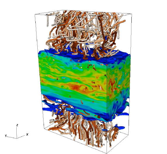
In Figure 1 we show a snapshot of our simulation run B3 in the saturated state of the MRI turbulence. We see clearly the large density fluctuations as a result of the vigorous MRI turbulence, and a substantial fraction of the gas is in supersonic motion. Meanwhile, there is a systematic vertical velocity at the vertical boundaries, indicating a strong outflow. In the following two sections, we discuss in detail the properties of the MRI turbulence and the outflow respectively.

3. Simulation Results: MRI Turbulence

One of the main diagnostics for the MRI turbulence is the ${r\phi}$ component of the stress tensor, consisting of the sum of Reynolds and Maxwell stresses,

$$T_{r\phi}^{\rm Rey}=\rho v_{x}v_{y}\ ,\qquad T_{r\phi}^{\rm Max}=-B_{x}B_{y}\ ,$$ (6)

and they characterize the rate of radial angular momentum transport. We are interested in the horizontally averaged vertical profiles (notated with an over bar, here $\overline{T}_{r\phi}$) of the stresses, and they are usually normalized by $\rho_{0}c_{s}^{2}$. Another useful measure is the mass weighted average of the stresses, normalized to the gas pressure (Shakura & Sunyaev, 1973)

$$\alpha=\frac{\int\overline{T}_{r\phi}(z)dz}{\int\bar{\rho}(z)c_{s}^{2}dz}\ ,$$ (7)

where $\alpha$ denotes either Reynolds or Maxwell stresses (with subscript), or their sum (without subscript), which characterizes the total rate of radial angular momentum transport in the disk.

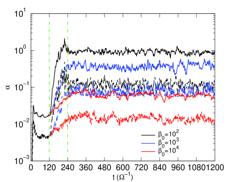
We show the evolution of $\alpha_{\rm Rey}$ and $\alpha_{\rm Max}$ in Figure 2. The total stress in the initial zero net-flux simulation saturates at $\langle\alpha_{\rm Rey}\rangle\approx 5.0\times 10^{-3}$ and $\langle\alpha_{\rm Max}\rangle\approx 2.0\times 10^{-2}$ respectively, consistent with previous works (e.g., Simon et al., 2012). The stresses increase steadily as we gradually add net vertical magnetic flux from $t=120\Omega^{-1}$, and saturate as full net flux is in place at $t=240\Omega^{-1}$. We wait for about another $20$ orbits and take the data from $t=360\Omega^{-1}$ to the end of the simulations at $t=1200\Omega^{-1}$ for all the time averages in this section, which amounts to about $130$ orbits. For our high-resolution run B3-hr, we consider data from $t=180\Omega^{-1}$ to the end of the simulation at $t=720\Omega^{-1}$, which amounts to about 85 orbits. Throughout this paper, we use angle bracket $\langle\cdot\rangle$ to denote time average.

In the saturated state, a common indicator for proper resolution of the MRI turbulence and convergence is the quality factor, defined as

$$Q_{j}\equiv\frac{2\pi|v_{Aj}|}{\Omega\Delta x_{j}},\ \quad{\rm where}\quad|v_{Aj}|\equiv\sqrt{\overline{B_{j}^{2}}/\overline{\rho}}\ ,$$ (8)

which is the ratio of a characteristic MRI wavelength to the grid scale. Here $j$ denotes either the $\hat{\boldsymbol{y}}$ or the $\hat{\boldsymbol{z}}$ dimension. Sano et al. (2004) found that $Q_{z}\gtrsim 6$ is required for the MRI turbulence to be well resolved. Hawley et al. (2011) further suggested that $Q_{z}\gtrsim 10$ and $Q_{y}\gtrsim 20$ suffice for properly resolving the MRI turbulence. Although these results are mainly based on either unstratified simulations or stratified simulations with zero net vertical magnetic flux, we take them as useful reference. In our simulations, the quality factors minimize at the disk midplane, where we find $\langle Q_{z}\rangle$ to be about $87$, $50$, $12$ for runs B2, B3 and B4 respectively, and $\langle Q_{y}\rangle$ is about $185$, $110$, $25$ for the three runs. For the high-resolution run B3-hr, we find $\langle Q_{z}\rangle\sim 110$ and $\langle Q_{y}\rangle\sim 285$. In all cases, the quality factors are well above the suggested value.

Figure 2.— Time history of mass weighted Maxwell (solid) and Reynolds (dashed) stresses from simulations B2, B3 and B4. They are restarted from the end of the zero net-flux simulation at $t=120\Omega^{-1}$. Net vertical magnetic field is added gradually to its full strength at $t=240\Omega^{-1}$.

3.1. Disk Structure

3.1.1 Vertical Profiles

Figure 3.— Vertical profiles of (from top to bottom) gas density $\langle\bar{\rho}\rangle$, plasma $\langle\bar{\beta}\rangle$, magnetic pressure of the toroidal field $\langle\bar{P}_{B,y}\rangle$, turbulent magnetic energy $\langle\bar{E}_{\rm B,turb}\rangle$ and turbulent kinetic energy $\langle\bar{E}_{\rm K,turb}\rangle$. In each panel, we show the profiles for runs B2 ($\beta_{0}=10^{2}$, solid), B3, ($\beta_{0}=10^{3}$ dashed) and B4 ($\beta_{0}=10^{4}$, dash-dotted) respectively, and the thin dashed lines correspond to run B3-hr ($\beta_{0}=10^{3}$ at high resolution).

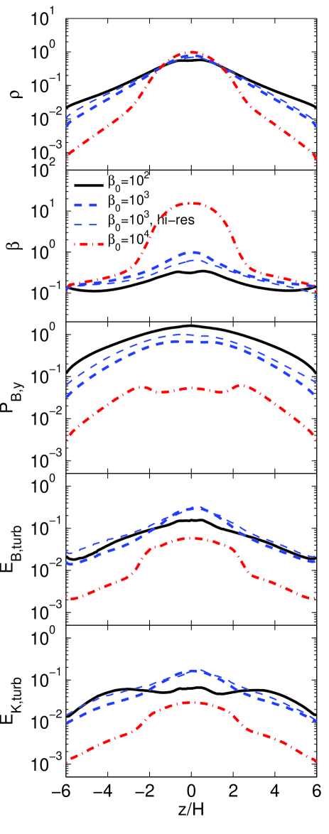
In the presence of a strong net vertical magnetic flux, the systems all saturate into very powerful MRI turbulence that substantially changes the structure of the disk. In Figure 3 we show the vertical profiles of various horizontally averaged quantities. The upper two panels are for gas density $\langle\bar{\rho}\rangle$ and plasma $\langle\bar{\beta}\rangle$ (ratio of gas to magnetic pressure). We see that the density profile deviates substantially from Gaussian due to strong magnetic support. Only for $\beta_{0}=10^{4}$, the Gaussian kernel is still present; while for $\beta_{0}\leq 10^{3}$, the entire disk becomes magnetically dominated, with plasma $\beta\lesssim 1$ everywhere. In all cases, the averaged plasma $\beta$ saturates at about 0.1 towards the disk surface, while in the extreme situation of $\beta_{0}=10^{2}$, plasma $\beta$ is about $0.1$ everywhere as MRI saturates. The magnetic pressure profile shows a large vertical gradient when $\beta\lesssim 1$ (as can be seen by dividing the first two panels of Figure 3). The magnetic pressure is dominated by contributions from the toroidal field (as can be compared with the third panel of the Figure), especially when $\beta_{0}\lesssim 10^{3}$. Correspondingly, the disk is substantially puffed up. We also note a potential caveat: the fact that the entire disk becomes magnetically dominated implies that in real disks, there can be strong magnetic pressure gradient support in the radial direction. This may lead to substantial sub-Keplerian rotation and in turn modifies the behavior of the MRI, a situation that requires global simulations to be properly addressed (see further discussions in Section 5.2).

In the lower two panels of Figure 3 we show the profiles of horizontally averaged turbulent magnetic energy $\langle\bar{E}_{\rm B,turb}\rangle$ and kinetic energy $\langle\bar{E}_{\rm K,turb}\rangle$. Here we have subtracted contributions from horizontally averaged mean fields and mean velocities at each vertical layer in the calculations: $\bar{E}_{\rm K,turb}\equiv\bar{E}_{K}-\bar{\rho}(\bar{v})^{2}/2$, $\bar{E}_{\rm B,turb}\equiv\bar{E}_{B}-(\bar{B})^{2}/2$. From the figure we see that for both magnetic and kinetic components, turbulent energy increases substantially by about one order of magnitude as $\beta_{0}$ changes from $10^{4}$ to $10^{3}$. As net vertical field increases further, to $\beta_{0}=10^{2}$, however, turbulent energy roughly stays at the same level as the $\beta_{0}=10^{3}$ case. This indicates that the strength of the MRI turbulence saturates as $\beta_{0}\lesssim 10^{3}$. On the other hand, the amplitude of the mean flow and mean magnetic field continue to increase with net vertical magnetic field, and their contributions to the total energy gradually dominate that from turbulent energy. We will discuss this fact further in Section 3.2. Here we note another caveat that in the presence of strong mean toroidal field at the level of equipartition or higher, the linear dispersion relation of the MRI is strongly modified by field curvature (Pessah & Psaltis, 2005), which is ignored in the shearing-box approximation, and again requires global simulations to be addressed properly.

Figure 4.— Vertical profiles of density fluctuations $\langle\delta\rho^{2}\rangle^{1/2}(z)$ normalized to horizontally averaged density $\langle\bar{\rho}\rangle$ for all simulation runs.

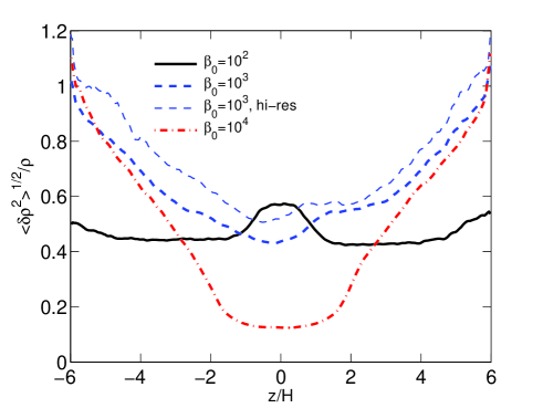
For $\beta_{0}\lesssim 10^{3}$, turbulence in all regions of the disk become trans-sonic or super-sonic, as one compares the profiles $\langle\bar{E}_{\rm K,turb}\rangle$ and $\langle\bar{\rho}\rangle$. This result implies strong compression and rarefaction, hence large density variations. Looking at the density field, we find that the density fluctuations in our simulations generally show elongated structure that is slightly tilted anti-clockwise from the azimuthal direction, indicating spiral density waves excited by the MRI turbulence (Heinemann & Papaloizou, 2009), although these structures are short lived due to the strong turbulence. To address such density variations, we measure the standard deviations of density fluctuations $\delta\rho$ in each horizontal layer, and normalize them to the horizontally averaged densities. The obtained profile of $\langle\delta\rho^{2}\rangle^{1/2}/\rho$ for all simulations are shown in Figure 4. We see that density variations are significant in all cases. For runs B3 and B4, the midplane density fluctuation increases with net magnetic flux, and reaches about $0.5$ for $\beta_{0}\lesssim 10^{3}$. The fluctuation level increases from the disk midplane, and reaches order unity at disk surface as the disk become more and more magnetically dominated. The case with $\beta_{0}=10^{2}$ show distinctive features from higher $\beta_{0}$ cases: except for a small bump around the disk midplane, the density fluctuation level stays roughly constant at about $0.5$. We note that the turbulent kinetic energy profile in run B2 is similar to that in run B3, while the density near disk surface in run B2 is a factor of several higher than run B3, indicating smaller turbulent velocity, hence the profile of $\langle\delta\rho^{2}\rangle^{1/2}/\rho$ for run B2 drops below that for run B3, which is essentially a reflection of weaker turbulence for run B2.

Figure 5.— Two-dimensional autocorrelation function (ACF) in the horizontal plane for magnetic energy fluctuations for our simulations B4 ($\beta_{0}=10^{4}$), B3, B3-hr ($\beta_{0}=10^{3}$) and B2 ($\beta_{0}=10^{2}$), from top to bottom. Left panels correspond to the ACFs for $|z|<2.5H$, while right panels are for $|z|>2.5H$. Note that the domain size for run B3-hr is slightly smaller.

3.1.2 Autocorrelation Function

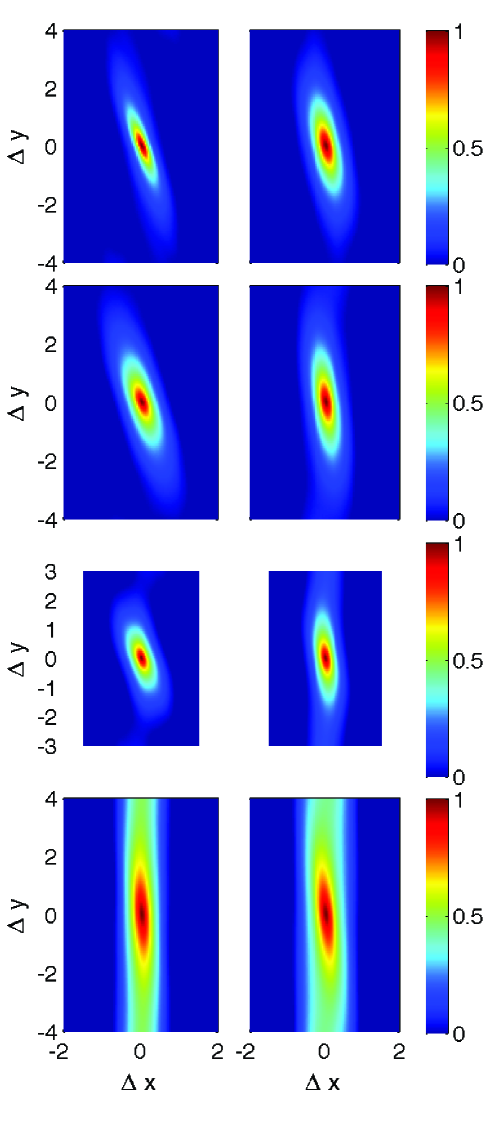
Another useful diagnostic of the MRI turbulence is the autocorrelation function (ACF) of kinetic and magnetic energy fluctuations, which is defined as (Guan et al., 2009; Simon et al., 2012)

$${\rm ACF}(E_{K,B},\Delta{\boldsymbol{x}})=\bigg{\langle}\frac{\int\delta{\boldsymbol{f}}(t,{\boldsymbol{x}})\cdot\delta{\boldsymbol{f}}(t,{\boldsymbol{x}}+\Delta\boldsymbol{x})d^{3}{\boldsymbol{x}}}{\int\delta f^{2}(t,{\boldsymbol{x}})d{\boldsymbol{x}}^{3}}\bigg{\rangle}_{t}\ ,$$ (9)

where $f$ denotes ${\boldsymbol{B}}$ for magnetic energy, and $\sqrt{\rho}{\boldsymbol{v}}$ for kinetic energy, the angle bracket denotes time average. Here we consider a two-dimensional ACF in the horizontal plane at some fixed vertical height $z$, and we subtract the horizontally averaged quantities in the evaluation of $\delta{\boldsymbol{f}}$: $\delta{\boldsymbol{f}}\equiv{\boldsymbol{f}}(x,y,z)-\bar{\boldsymbol{f}}(z)$. This is necessary as the mean flow and mean field can become particularly strong in the presence of net vertical magnetic field.

In Figure 5, we show the ACFs for magnetic energy fluctuations in all our simulations B2, B3, B3-hr and B4, for both near the midplane region (left, for $z\leq 2.5H$) and the disk surface (right, $2.5H\leq z\leq 5H$). The ACFs for the kinetic energy exhibits similar patterns, hence we do not involve a separate figure to show them. The ACF for run B4 at midplane where the net vertical magnetic flux is relatively small ($\beta_{0}=10^{4}$) is very similar to that found in zero net-flux simulations (Guan et al., 2009; Simon et al., 2012), containing a narrow and elongated centroid that is tilted with respect to the azimuthal axis by about $\zeta_{B}\sim 15^{\circ}$. Such a tilt angle is related to the empirical correlation between the plasma $\beta$ and the stress parameter $\alpha\approx 1/2\beta$ (Guan et al., 2009; Bai & Stone, 2011), which also applies for the midplane region of our run B4 as we can compare Figures 3 and 6. Moving up to the disk surface, we find that the centroid becomes broader in the upper layer, and the tilt angle also becomes smaller. These features indicate longer correlation length in the radial direction, as well as more isotropy in the magnetically dominated disk corona. The ACFs in run B3 at the midplane has similar tilt angle as in run B4, typical for MRI turbulence, while at both midplane and corona, the peaks in the ACFs are as broad as the corona region of run B4, which is in line with the fact that the entire disk has become magnetically dominated.

Our run B2 with $\beta_{0}=100$ exhibits an extreme situation: fluctuations are highly elongated in the azimuthal direction, with the measured correlation length comparable to the azimuthal size of our simulation box, which might suggest that our azimuthal box size is not sufficient to properly resolve the MRI turbulence. Nevertheless, the shape of the ACF indicates that the fluctuations are quasi-axisymmetric (which is also evident as one views the raw simulation data), and the radial fluctuations are well fitted into our simulation box.

3.1.3 Numerical Convergence

Due to the large computational cost, we have not carried out a full resolution study in this paper. However, we do expect our simulation results to converge in runs B2 and B3-hr where we have adequate resolution to properly resolve the linear MRI modes as suggested by Latter et al. (2010). Based on the quality factor criterion (Hawley et al., 2011), we expect all our simulations to well resolve the MRI turbulence. Below we compare the results between our simulation runs B3 and B3-hr and briefly discuss about numerical convergence.

We see from Figure 5 that the shape of the ACFs in our runs B3-hr and B3 are similar, but the ACF in run B3-hr is more centrally-peaked than its low-resolution counterpart. Since the ACF is simply the Fourier transform of the power spectrum, this indicates that the high-resolution run gives a flatter power spectrum with more power on the small scales. In addition, comparing various profiles in Figure 3 between runs B3 and B3-hr, we see again that the profiles are very similar, with higher resolution giving slightly higher turbulent energy. This is also reflected in Table 2 where the Shakura-Sunyaev $\alpha$ from run B3-hr is about $25\%$ higher. Similarly, in Figure 4, we see that run B3-hr leads to slightly larger density fluctuations. Later in Figure 9, slightly higher mass outflow rate is achieved in run B3-hr.

The systematically higher saturation amplitude of the MRI in the high-resolution run discussed above might suggest that our simulations for $\beta_{0}=10^{3}$ have not fully reached numerical convergence. However, such higher saturation amplitude may not be due to under-resolved MRI turbulence, and several other factors are likely to play a role. While slightly smaller horizontal box size in run B3-hr can be a potential cause, the fact that the peaks of the ACF are well contained in the box makes it somewhat unlikely (Simon et al., 2012). Another possibility is that in stratified MRI simulations, the property of the MRI turbulence is largely affected by the dynamo process (see detailed study in Section 3.3), which generates strong mean toroidal field that changes sign over time. It appears that the instantaneous large-scale toroidal field generated in run B3-hr is on average stronger than that in run B3, as can be judged from Figure 7, and both are above equipartition field strength. Such larger mean toroidal field leads to stronger magnetic support to the disk, resulting in slightly different vertical disk structures between the two runs B3 and B3-hr. In this respect, one should be careful when discussing the issue of convergence, since comparing turbulent properties between simulations with different disk structures can be misleading. Since the mechanism of the dynamo is far from being understood, and the dynamo in the presence of strong net vertical flux behaves very differently from the case with zero net vertical flux, we defer this convergence issue for future study.

In sum, although quantitative differences exist between runs B3 and B3-hr, the physical properties of the MRI turbulent disk from the two runs all agree with each other. We therefore consider both runs as valid representations of the physical system, with run B3-hr as a more accurate model.

3.2. Energetics and Angular Momentum Transport

There are two sources of angular momentum transport in accretion disks, namely, the radial transport (or re-distribution) via turbulence and the vertical transport via disk wind. We study them separately in this subsection and then briefly discuss about the energetics in our simulations.

3.2.1 Radial Transport of Angular Momentum

Figure 6.— Vertical profiles of Maxwell stress (solid) and Reynolds stress (dashed) for runs B2, B3-hr and B4 (from top to bottom panels). In each panel, we show the total stress (bold) as well as contribution from turbulent fluctuations (thin). The stresses are normalized by $\rho_{0}c_{s}^{2}$.

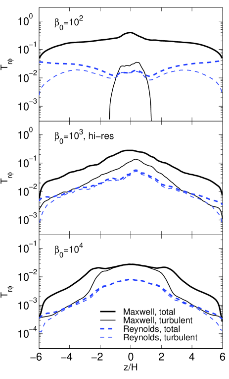
The radial transport of angular momentum is characterized by the $\alpha$ parameters defined in equation (7). In Figure 6, we show the vertical profiles of Maxwell and Reynolds stresses for all our simulations. Both the Maxwell and Reynolds stresses increases monotonically with net vertical magnetic flux, and approaches a few times $0.1\rho_{0}c_{s}^{2}$ for $\beta_{0}=10^{2}$. In the mean time, the profile gradually changes from centrally peaked for large $\beta_{0}$, to a more or less flat profile at $\beta_{0}=10^{2}$. In particular, the slope of the wing beyond $\pm 2H$ becomes more level as $\beta_{0}$ decreases. We can further compare our run B4 with zero net vertical flux stratified MRI simulations (Stone et al., 1996; Miller & Stone, 2000; Guan & Gammie, 2011; Simon et al., 2012), where the slope of the wing is further steeper. These results suggest a general trend that the surface region plays a more and more important role in the radial angular momentum transport as the net vertical magnetic field increases. Also, we see that the Maxwell stress is always larger than the Reynolds stress, but the Reynolds stress becomes more and more important toward disk surface.

To further decode the mechanism for the radial transport of angular momentum, we separate the contributions from the mean field/mean flow ($\langle\bar{\rho}\bar{v}_{x}\bar{v}^{\prime}_{y}\rangle$ or Reynolds stress and $\langle-\bar{B}_{x}\bar{B}_{y}\rangle$ for Maxwell stress) and the turbulent stress (the rest). We remind the reader that we compute the mean stress from horizontally averaged quantities in each snapshot and then take the time average. As net vertical field increases, the turbulent component increases steadily with net field and saturates for $\beta\lesssim 10^{3}$ in a way similar to the turbulent energy density profile in Figure 3. There are two intriguing features Figure 6. First, in the disk surface region (near our vertical boundary), the stress is dominated by the mean field/mean flow components (i.e., magnetic breaking) rather than turbulence, and the contribution from the mean field/mean flow components rapidly increases as net field increases. In run B4, the mean field component dominates the wings of the Maxwell stress, while in runs B3-hr (and B3), the mean field component dominates the entire disk. Second, for sufficiently strong background magnetic field $\beta_{0}\lesssim 10^{2}$, the turbulent stress become completely unimportant at all locations, and the turbulent Maxwell stress can even become negative. Interestingly, the central region where the turbulent Maxwell stress is positive coincides with the bump in the density fluctuation (Figure 4).

The decline of the turbulent component and rise of the mean field/mean flow component of the stress as one increases net vertical flux strongly contrast with conventional unstratified shearing-box simulations. In those simulations, the initial net toroidal magnetic field is mostly set to zero. Although the net toroidal magnetic flux is a not conserved quantity, it generally stays very close to zero for the duration of the simulations. With stratification, the large-scale toroidal field evolves substantially and for $\beta_{0}\lesssim 10^{3}$, it well exceeds equipartition strength (see Figures 7 and 12). Although the linear growth of the MRI is not directly coupled to the toroidal field, the non-linear saturation certainly depends on it (Hawley et al., 1995). Therefore, it is not appropriate to compare unstratified MRI simulations with stratified simulations with the same $\beta_{0}$ unless the unstratified simulation contains a substantial net toroidal magnetic field.

Table 2Energetics and Angular Momentum Transport.

Run	$\langle\alpha_{\rm Max}\rangle$	$\langle\alpha_{\rm Rey}\rangle$	$\langle T_{z\phi}^{\rm Max}\rangle$	$\langle T_{z\phi}^{\rm Rey}\rangle$	$P_{\rm sh}$	$\dot{E}_{K}$	$\dot{E}_{P}$	$\dot{m}_{w}$
B2	0.92	0.12	0.061	0.048	3.90	0.89	1.26	0.0944
B3	0.37	0.077	0.0085	0.0041	1.69	0.079	0.15	0.0138
B3-hr	0.47	0.086	0.010	0.0046	2.08	0.086	0.21	0.0160
B4	0.061	0.014	0.00072	0.00036	0.28	0.0065	0.010	0.0013

Note: All in natural units, with $\rho_{0}=c_{s}=\Omega=1$.

Integrating the stresses one obtain the $\alpha$ parameter defined in (7), and the results are listed in Table 2. The $\alpha$ parameter increases monotonically with net magnetic flux, from a total of about $\langle\alpha\rangle\approx 0.075$ for $\beta_{0}=10^{4}$ to $\langle\alpha\rangle\approx 1.0$ for $\beta_{0}=100$, The ratio of $\langle\alpha_{\rm Max}\rangle$ to $\langle\alpha_{\rm Rey}\rangle$ increases from about 4 for $\beta_{0}=10^{4}$, which is similar to that in zero net vertical flux simulations (e.g., Davis et al., 2010), to about 7 for $\beta_{0}=10^{2}$, which is mainly due to an increasing contribution from the mean (rather than turbulent) magnetic field.

We note that in run B2, the Maxwell stress only decreases very slowly with height, while the Reynolds stress even increases with height, making the volume integrated stress limited by the vertical extent of our simulation box. However, we argue that increasing the box size does not necessarily improve the situation. In this case, the radial angular momentum transport is dominated by the mean field and mean flow. As we shall discuss in Section 4, the strength of the large-scale mean field at disk surface is intimately connected to the global condition of the disk and can not be determined in the local shearing-box approch. Therefore, uncertainty still remains as one uses a taller box. The measured $\langle\alpha\rangle$ value for run B2 should be only taken as a reference.

3.2.2 Vertical Transport of Angular Momentum

Angular momentum can also be extracted from the disk directly in the vertical direction through outflow and magnetic fields, which is determined by the $z\phi$ components of the Reynolds and Maxwell stresses exerted at vertical boundaries

$$\begin{split}T_{z\phi}^{\rm Rey}&=(\rho v_{y}v_{z})|_{\rm bot,top}\ ,\\ T_{z\phi}^{\rm Max}&=(-B_{y}B_{z})|_{\rm bot,top}\ ,\\ \end{split}$$ (10)

where in practice subscripts _bot and _top mean that we measure these quantities at the last layer of the top and bottom of the computational domain. The torque exerted by the wind stresses can be obtained by simply multiplying $\langle T_{z\phi}^{\rm Rey}\rangle$ and $\langle T_{z\phi}^{\rm Max}\rangle$ by the radius $R$. Including the contributions from radial and vertical transports, the accretion rate can be approximately written as

$$\dot{M}=\dot{M}_{r}+\dot{M}_{z}\approx\frac{2\pi}{\Omega}\int dzT_{r\phi}+\frac{4\pi R}{\Omega}T_{z\phi}\bigg{|}^{\infty}_{-\infty}\ ,$$ (11)

where $\dot{M}_{r}$ and $\dot{M}_{z}$ represent contributions to the accretion rate from radial and vertical transport respectively. Qualitatively, one may replace the vertical integral $\int dz$ by the disk scale height $H$. We see that given the same level of stress $T_{r\phi}$ and $T_{z\phi}$, vertical transport is more efficient than radial transport by a factor of about $R/H$.

Being a local shearing-box simulation, however, $R$ is unspecified, and moreover, the location of the central object is unspecified (can either at inner or outer $\hat{\boldsymbol{x}}$ direction), making the sign of $R$ ambiguous. A physical disk wind requires that the sign of $T_{z\phi}$ on the two vertical boundaries be the opposite and are steady, and is closely related to the symmetry of the wind solution as we will discuss in detail in Section 4.3. In this subsection, we only consider the absolute value of $T_{z\phi}$ and average it over the two vertical boundaries (i.e., assuming the flow structure and magnetic configuration has the physical geometry), hence the relative importance between radial and vertical transport can be rewritten as

$$\frac{\dot{M}_{r}}{\dot{M}_{z}}=\frac{\sqrt{2\pi}}{4}\frac{H}{R}\frac{\alpha}{|T_{z\phi}^{\pm\infty}|/\rho_{0}c_{s}^{2}}\ .$$ (12)

We list the values of $T_{z\phi}^{\rm Rey}$ and $T_{z\phi}^{\rm Max}$ from each simulation run in Table 2, with both normalized by $\rho_{0}c_{s}^{2}$. The wind stresses appear to depend more sensitively on $\beta_{0}$, and increase by about two orders of magnitude from $\beta=10^{4}$ to $\beta=100$. This may suggest the importance of wind transport relatively to turbulent transport increases with net vertical field. Taking $H/R=0.1$, we find that wind transport, if present, should be small (less than $25\%$) compared with radial transport for $\beta_{0}=10^{4}$, which is consistent with the results by Fromang et al. (2012). It would become more or less comparable to radial transport for $\beta_{0}=10^{3}$, while it would dominate radial transport for $\beta_{0}=10^{2}$. In addition, the contributions from Maxwell $T_{z\phi}^{\rm Max}$ and Reynolds $T_{z\phi}^{\rm Rey}$ components are roughly $2:1$ in runs B3 and B4, while the Reynolds component becomes more important for run B2. However again, as we shall discuss in Section 4, the wind stress can only determined from global approach, while our measured $\langle T_{z\phi}\rangle$ values should also be taken as a reference.

3.2.3 Energetics

Using an isothermal equation of state, total energy is not conserved in the simulation. However, it is important to examine the energy budget for consistency such that the work done by the Keplerian shear (i.e., from radial shearing-box boundaries) exceeds the energy loss from the vertical boundaries, with the rest of the energy presumably escape from the disk in the form of radiation.

In ideal MHD, the energy flux is given by

$${\boldsymbol{F}}_{E}=\bigg{(}\frac{1}{2}\rho u^{2}+\epsilon+P_{\rm gas}+B^{2}\bigg{)}{\boldsymbol{u}}-({\boldsymbol{B}}\cdot{\boldsymbol{u}}){\boldsymbol{B}}\ ,$$ (13)

where $\epsilon$ is the internal energy. Consider the net energy flux entering the two sides of the radial boundaries, where we compute ${\boldsymbol{F}}_{E}\cdot{\boldsymbol{e}}_{x}$ and integrate over height and azimuth. Note that ${\boldsymbol{u}}$ contains background shear, and one should shift $u_{y}$ by $3\Omega L_{x}/2$ between the two boundaries. Correspondingly, only terms containing ${\boldsymbol{u}}$ contribute, while all other terms cancel due to the shear-periodic boundary condition. The non-vanishing terms turn out to be Maxwell and Reynolds stress, and the work done by the radial boundaries per unit horizontal area per unit time read

$$P_{\rm sh}=\frac{1}{L_{x}L_{y}}\int\frac{3}{2}\langle\rho v_{x}v_{y}-B_{x}B_{y}\rangle\Omega L_{x}dydz=\frac{3}{2}\Sigma c_{s}^{2}\Omega\langle\alpha\rangle\ ,$$ (14)

where $\Sigma=\int\langle\bar{\rho}(z)\rangle dz$ is the column density.

The energy loss from vertical boundaries is given by

$$\dot{E}=\dot{E}_{K}+\dot{E}_{P}=\bigg{[}\rho\bigg{(}\frac{v^{2}}{2}+c_{s}^{2}\bigg{)}{\boldsymbol{v}}-({\boldsymbol{v}}\times{\boldsymbol{B}})\times{\boldsymbol{B}}\bigg{]}\cdot{\boldsymbol{n}}\bigg{|}_{\rm top+bot}\ ,$$ (15)

where ${\boldsymbol{n}}$ is the unit vector pointing away from the disk in the vertical direction, and we sum over contributions from the top and bottom vertical boundaries. The first terms in the bracket represent the kinetic energy loss and the $PdV$ work done by the mass outflow, and the second term represents energy loss from the Poynting flux . We have ignored the energy loss term associated with internal energy due to the mass outflow, since we keep feeding mass to the system which balances this term exactly. This term is comparable to the $PdV$ work term which, as we shall see, is always small compared with the total $\dot{E}$ (hence our mass addition do not substantially alter the energy balance).

In Table 2 we also list the values of $P_{\rm sh}$, $\dot{E}_{K}$ and $\dot{E}_{P}$, normalized in natural units. We see that $P_{\rm sh}$ is always larger than the sum of $\dot{E}_{K}$ and $\dot{E}_{P}$, hence energy conservation is not violated. Also, we see that $\dot{E}_{P}$ is always larger than $\dot{E}_{K}$ by a factor of about $1.5$ to $2$, hence Poynting flux dominates energy loss. In addition, under the assumption of isothermal equation of state adopted in our simulations, we find that as net vertical magnetic field increases, $\dot{E}_{K}+\dot{E}_{P}$ roughly increases as $1/\beta_{0}$, which is much faster than the rate $P_{\rm sh}$ increases. This may suggest radiative efficiency decreases as a larger fraction of work done by the shear is converted into the wind energy loss.

3.3. Dynamo Activities

Figure 7.— The time evolution of the horizontally averaged profiles of toroidal magnetic field in all simulation runs, from top to bottom: B2, B3, B3-hr and B4. Here we mark $t^{\prime}=0$ as the time when full net vertical flux is added ($t=240\Omega^{-1}$ for B2, B3 and B4, $t=0$ for B3-hr). The white contours mark plasma $\beta=1$.

It is well known in stratified shearing-box simulations with zero net vertical magnetic flux that the mean toroidal field component experiences periodic flips on the time scale of $10$ orbits (e.g., Brandenburg et al., 1995; Shi et al., 2010; Davis et al., 2010; Simon et al., 2012). Since a zero background vertical field does not give any instability on its own in the linear theory, the MRI activity in these simulations together with the periodic flips strongly suggest that a magnetic dynamo is in operation. It is generally believed that shear, turbulence and large scale azimuthal field are responsible for sustaining the dynamo cycles (Vishniac & Brandenburg, 1997; Yousef et al., 2008; Lesur & Ogilvie, 2008; Gressel, 2010), yet the detailed mechanism remains unsettled.

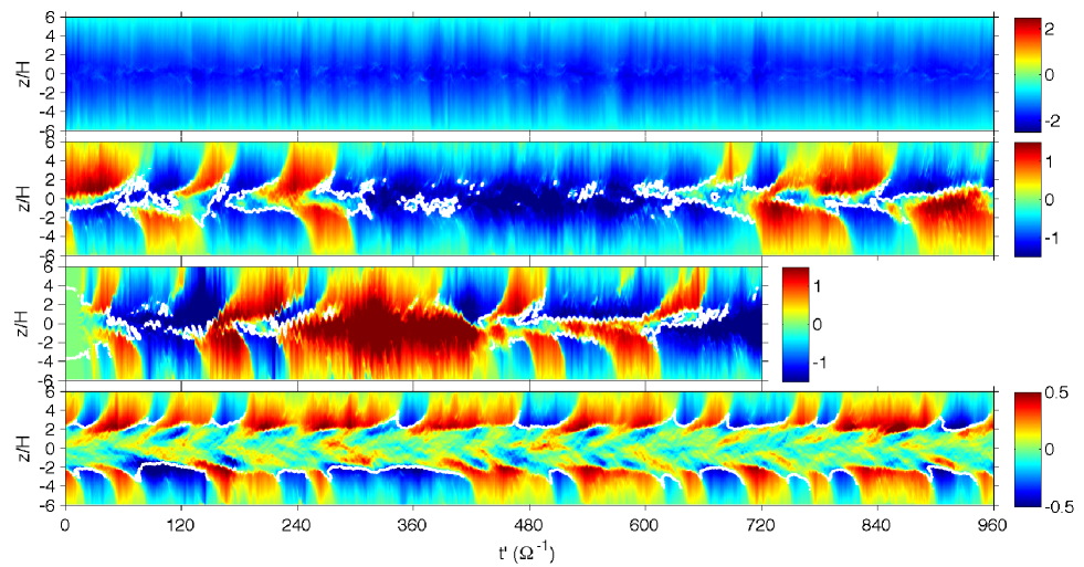
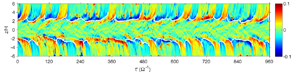
In the presence of net vertical magnetic field, the MRI can be sustained from the linear modes hence a dynamo is not necessary to explain the turbulence. With very weak vertical net magnetic flux, dynamo behavior was also observed in Suzuki & Inutsuka (2009), Suzuki et al. (2010) and Fromang et al. (2012), whose simulations correspond to $\beta_{0}=10^{4}-10^{6}$, although it was not studied in detail. Our simulations allow us to systematically study the evolution of the MRI dynamo with net vertical magnetic flux. In Figure 7, we show the space-time plot of the horizontally averaged azimuthal magnetic field for all our simulation runs. It is obvious that for $\beta_{0}=10^{4}$, the mean azimuthal field still undergoes cyclic oscillations between positive and negative signs, while for $\beta_{0}=100$, the dynamo behavior disappears, where the mean azimuthal field in the entire simulation box is completely dominated by one sign at all times. The case with $\beta_{0}=10^{3}$ is somewhat marginal, where the dynamo-like behavior is present for part of the time while for the rest of the time the mean azimuthal field is predominantly one sign.

In zero net vertical flux stratified shearing-box simulations (see Figure 15 of Simon et al., 2012 for a most clear rendering), the dynamo pattern is highly repeatable in the space-time plot, also known as the “butterfly diagram”, with a well-defined of period about 10 orbits. The dynamo cycles in our run B4 with $\beta_{0}=10^{4}$, however, is highly irregular. Such behavior is also observed in Fromang et al. (2012). Further including the marginal case of run B3 with $\beta_{0}=10^{3}$, we see that there is a systematic trend that as net vertical field increases, the dynamo cycle weakens by becoming more irregular with less periodicity. The flipping of mean azimuthal field becomes more sporadic, and the mean time interval for field flipping also becomes longer. As $\beta_{0}$ reaches below $10^{3}$, the flipping time interval virtually becomes infinity, and the dynamo is completely quenched.

We note that the most unstable linear MRI mode is properly resolved in run B2, which does not show dynamo behavior, but may not be well resolved in runs B3 and B4, which show dynamo activities. Hence question arises on whether the dynamo activity depends on the proper resolution of the linear MRI modes. Our run B3-hr, which is the same as run B3 but properly resolves the most unstable MRI mode, is designed to clarify this potential ambiguity. We see that the space-time pattern for the mean azimuthal field is very similar in the two runs: dynamo activity appears only part of the time. This comparison further justifies that the dynamo behaviors observed in our simulations are real.

It is natural to ask about what physical effects control the dynamo activities. Phenomenologically, we see that in the presence of the dynamo, the disk is separated into two distinct regions, namely the region near the midplane with relatively weak magnetic field where the dynamo appears to be developed, and a highly magnetized region outside. In Figure 7, we have overplotted white contours that mark the total plasma $\beta=1$ (i.e., total magnetic pressure equals the gas pressure). Remarkably, these white contours perfectly separate the two regions for both runs B3 and B4, while for run B2, the entire disk is magnetically dominated hence there is no contour at all times. It is intriguing to notice that the dynamo is present whenever the magnetic field strength in the disk midplane region is below equipartition strength.

Meanwhile, the criterion of $\beta=1$ also applies to magnetic buoyancy (i.e., interchange and Parker-type instabilities, Newcomb, 1961; Parker, 1966) as discussed in a number of zero net-flux simulations (Blaes et al., 2007; Shi et al., 2010; Guan & Gammie, 2011; Simon et al., 2011). With isothermal equation of state, and assuming zero mean vertical field, the fluid is buoyantly unstable if the magnetic energy density decreases with height (Guan & Gammie, 2011). It turns out that the magnetic field strength tends to be constant in the gas pressure dominated disk midplane regions, presumably due to efficient turbulent mixing, while it falls off with height in the magnetically dominated corona. Correspondingly, for regions with $\beta<1$, the fluid is unstable due to magnetic buoyancy, while for regions with $\beta>1$, the fluid is buoyantly (marginally) stable and dynamo activities produce cyclic alternations of the mean magnetic field. Although the analysis of the Parker instability in previous works assumes zero mean vertical field, it continues appear to be valid in our simulations with net vertical field, which is likely because the net vertical field in our simulations is much weaker (by at least a factor of $10$) than the mean azimuthal field.

The strong azimuthal magnetic field in our simulations with $\beta_{0}\lesssim 10^{3}$ is to some extent similar to the simulations performed by Johansen & Levin (2008). They initiated their simulations by a pure azimuthal field with equipartition strength (with zero net vertical magnetic flux), and found that the interplay between the Parker instability at disk surface layer and the MRI near the midplane effectively produces a magnetic dynamo, and the azimuthal flux is well confined to the disk. Simulations of Gaburov et al. (2012) for the tidal disruption of a molecular cloud approximately realize the situation. The key difference in our case is that a strong outflow is produced in the presence of net vertical magnetic field (see Section 4), hence azimuthal flux continuously escape the simulation box and has to be continuously generated within the disk. Therefore, although Parker instability is likely to be present in the entire disk when $\beta_{0}\lesssim 10^{3}$, the dynamo mechanism of Johansen & Levin no longer operates in the presence of strong net vertical magnetic field. On the other hand, magnetic dissipation due to the Parker instability is likely to play an important role on the thermal structure of the disk (Uzdensky, 2012), which deserves future exploration.

4. Simulation Results: Outflow

It has been found in Suzuki & Inutsuka (2009) and Suzuki et al. (2010) that the inclusion of a net vertical magnetic field leads to strong mass outflow in shearing-box MRI simulations, and the rate of the mass outflow is approximately proportional to $1/\beta_{0}$. The mass outflow was interpreted as the launching of a wind from the disk and would potentially connect to a Blandford & Payne (1982) type global disk wind. The connection between MRI-driven outflow and global disk wind has been further investigated by Fromang et al. (2012), who focused on the case with $\beta_{0}=10^{4}$. They argue that the MRI is able to launch the magnetocentrifugal wind that is strongly time-dependent. Similar conclusion has been made by Lesur et al. (2012) for the case with $\beta_{0}\sim 10$, where there is only one single MRI mode fitted into the disk with a physical symmetry for the wind, and secondary instabilities are likely to make it time-dependent. Very strong outflows are also observed in our simulations. However, we argue that the outflow seen in shearing-box MRI simulations is unlikely to be directly connected to a global disk wind, as we elaborate below.

4.1. Structure of the Outflow

4.1.1 Critical Points

The global disk wind model by Blandford & Payne (1982) states that when the magnetic field at the surface of a thin disk is inclined relative to the disk normal for more than $30^{\circ}$, outflowing gas can be accelerated centrifugally along field lines, extracting angular momentum from the disk, and is gradually collimated by the magnetic hoop stress. A crucial ingredient of this picture is the wind launching/mass loading from the disk, which is intrinsically connected to the gas dynamics in the disks. The wind launching process has been studied analytically under the local shearing-box approximation (Wardle & Koenigl, 1993; Ogilvie & Livio, 2001; Ogilvie, 2012), where all the radial gradients except the shear are omitted to reduce the problem to fully one-dimensional (1D). The 1D solutions are then matched to global wind solutions, where the mass loading rate is determined as an eigen-value problem.

Figure 8.— Horizontally-averaged vertical velocity profiles for fiducial resolution simulations B2, B3 and B4 with $\beta_{0}=10^{2}$ (solid), $10^{3}$ (dashed) $10^{4}$ (dash-dotted) respectively. Also marked are the locations of Alfvén points (solid dots) and slow magnetosonic points (circles). The fast magnetosonic points are beyond the simulation domain.

A physical wind solution should pass three critical points, namely, the slow and fast magnetosonic points, and the Alfvén point. In the 1D (laminar) model, they are given by

$$v_{z}^{2}=\frac{1}{2}(c_{s}^{2}+v_{A}^{2})\pm\frac{1}{2}\sqrt{(c_{s}^{2}+v_{A}^{2})-4c_{s}^{2}v_{Az}^{2}}\ ,$$ (16)

for fast and slow magnetosonic points, and

$$v_{z}=\pm v_{Az}\ ,$$ (17)

for the Alfvén point, where $v_{Az}=\sqrt{B_{z}^{2}/\rho}$ is the vertical component of the Alfvén velocity, and $v_{A}$ is the full Alfvén velocity. The requirement that the flow passes smoothly through these critical points poses three eigen-value problems that would determine three physical quantities, such as the mass loading rate and the field inclination at disk surface. In the local shearing-box approach, the fast magnetosonic point, and sometimes the Alfvén point, are sufficiently high above the disk where the local approximation no longer applies, and they need to be captured in the global models. The lack of one or two critical points implies that the solution obtained within the computational domain has one or two degrees of freedom.

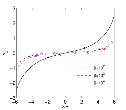
In Figure 8, we show the time and horizontally averaged profiles of the gas vertical velocity as a function of height. In all cases, the vertical velocity rapidly increases towards disk surface, and becomes transsonic or supersonic as the flow leaves the simulation box. We also calculate the location of the critical points based on equations (16) and (17), where the Alfvén velocity is based on the time average of the absolute value of the horizontally averaged the magnetic field. We find that for all cases, the fast magnetosonic points are beyond our simulation box (the fast magnetosonic speed is about $3c_{s}$ or larger at vertical boundaries), while the Alfvén (marked in the Figure) and slow magnetosonic points are well contained in the box. This fact means that the flow structure is not fully determined and has one degree of freedom.

4.1.2 Conservation Laws

Figure 9.— Top: time averaged vertical profile of mass outflow rate normalized to the mean vertical magnetic field (or $\kappa$, see Equation 18) for all our simulation runs. Bottom: time averaged mass loss rate from the simulation domain as a function of net vertical flux. Thick/thin symbols correspond to fiducial/high resolution simulations (B3-hr/B3).

It is well known that for a laminar magnetized wind, the gas follows the magnetic field lines, and the flow is characterized by a number of conserved quantities along the streamlines (Blandford & Payne, 1982; Pelletier & Pudritz, 1992). These conservation laws provide very useful diagnostics that help us understand the mechanism for the launching and acceleration of the outflow, as well as the angular momentum transfer processes. The forms of these conservation laws in the shearing-box framework are derived in Lesur et al. (2012). In shearing-box, it was shown that poloidal gas streamlines do not necessarily follow exactly the poloidal field lines, which brings new terms to the conservation law. Nevertheless, the difference is generally small. Since strong turbulence are present in all our simulations while these conservation laws are derived for a laminar flow, they only hold approximately and serve for diagnostic purpose.

The starting point is mass conservation, where

$$\overline{\rho v_{z}}={\rm const}\equiv\kappa\overline{B}_{z}\ ,$$ (18)

where overline indicates horizontal average, and $\kappa$ is constant. We show the profile of $\overline{\rho v_{z}}/\overline{B}_{z}$ (or $\kappa$) for all our simulation runs in the top panel of Figure 9. Because we constantly add mass to the simulation box to maintain steady state, the vertical profile of $\overline{\rho v_{z}}$ does not become flat until beyond $z\sim\pm 3H$. There is some asymmetry in the high-resolution run B3-hr, which is most likely due to its shorter run time and the lack of statistics. The asymptotic values of $\overline{\rho v_{z}}$ are used to calculate the mass loss rate $\dot{m}_{w}$ from the simulations

$$\dot{m}_{w}\equiv\langle\overline{\rho v_{z}}\rangle|_{\rm top}-\langle\overline{\rho v_{z}}\rangle|_{\rm bot}\ ,$$ (19)

and we have listed the value of $\dot{m}_{w}$ in Table 2. Further details about the mass outflow rate will be discussed in Section 4.2.

As long as $\kappa$ is constant, as valid beyond $z\pm 3H$ in our simulations, specific angular momentum and energy are conserved along streamlines. Following Lesur et al. (2012), the specific angular momentum reads

$$f\equiv{\mathcal{L}}-\frac{\bar{B}_{y}}{\kappa}\ ,$$ (20)

where ${\mathcal{L}}\equiv v_{y}+\Omega x/2$ is the fluid part of the specific angular momentum. The partition between ${\mathcal{L}}$ and $\bar{B}_{y}/\kappa$ then describes the angular momentum exchange between gas and magnetic field.

Energy conservation is given by the Bernoulli invariant, which reads (Lesur et al., 2012, without correction terms)

$$\begin{split}E_{\rm Ber}&=E_{K}+E_{T}+E_{\phi}+E_{B}\\ &=\frac{\bar{u}^{2}}{2}+c_{0}^{2}\log(\bar{\rho})+\phi-\frac{\bar{B}_{y}v_{y}^{*}}{\kappa}\ ,\end{split}$$ (21)

where $E_{\rm Ber}$ represents the specific energy along a streamline, with the four terms denoting kinetic energy, enthalpy, potential energy and the work done by the magnetic torque, respectively, and

$$v_{y}^{*}\equiv\bar{u}_{y}-\kappa\bar{B}_{y}/\bar{\rho}\ .$$ (22)

Note that the full velocity ${\boldsymbol{u}}$ (rather than ${\boldsymbol{v}}$) enters $E_{K}$, and the potential energy for the shearing-box is

$$\phi=-\frac{3}{2}\Omega x^{2}+\frac{1}{2}\Omega z^{2}\ .$$ (23)

We extract the mean flow of the gas and integrate to obtain the streamline. Because the disk midplane regions are generally the most turbulent with $\kappa$ varying with height, we do not expect conservation laws to hold in these regions region and only trace streamlines from $z=3H$ to $z=6H$, setting $x=0$ at $z=3H$ (note that by construction the conservation laws do not depend on the choice of the zero point of $x$). This treatment covers the most interesting surface regions of the disk where the launching and acceleration of the outflow take place. For illustration purpose, we only consider run B2 and B4. For run B2, the large-scale flow and magnetic structures are more or less steady (as seen from Figure 7), hence we take the long-term average to obtain the desired physical quantities along streamlines. For run B4, due to the dynamo activities, we only pick up a short period between $t^{\prime}=560\Omega^{-1}$ and $t^{\prime}=600\Omega^{-1}$, where the magnetic structure in the upper side of the disk is quasi-steady, as judged from Figures 7 and 11.

Figure 10.— Energy (top) and angular momentum (bottom) along a streamline in the disk surface from $z=3H$ to $6H$ for run B2 (left, with long time average) and B4 (right, averaged between $t^{\prime}=560\Omega^{-1}$ and $t^{\prime}=600\Omega^{-1}$). For the energy plot, the various terms in Equation (21) are represented by: $E_{\rm Ber}$ (black dashed), $E_{K}$ (blue solid), $E_{T}$ (magenta solid), $E_{B}$ (green solid) and $\phi$ (red solid). For the angular momentum plot, the various terms in Equation (20) are represented by: $f$ (black dashed), ${\mathcal{L}}$ (blue solid), $-\bar{B}_{y}/\kappa$ (red solid).

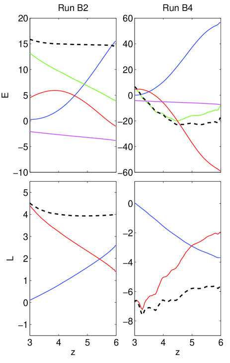
In Figure 10 we show the vertical profiles of individual terms in the specific energy and angular momentum for streamlines obtained from runs B2 and B4. We see from the black dashed lines that energy and angular momentum are approximately conserved beyond about $4H$ for both cases. The rise of the blue lines in the energy plots indicate flow acceleration. This is mostly compensated by the reduction of potential energy (red) and work done by the magnetic torque (green). Similarly, in the bottom panels of Figure 10, we see that the increase of fluid angular momentum is compensated by the reduction of magnetic torque. Therefore, it becomes clear that the acceleration is magnetocentrifugal in nature. Note that the role played by centrifugal potential $\phi$ and the magnetic torque $-\bar{B}_{y}v_{y}^{*}/\kappa$ can be exchanged by shifting the zero point of $x$, hence they represent the same effect. For example, if we were to trace the streamlines from the disk midplane for the case of run B2, then we would found that the acceleration is almost completely due to the centrifugal potential, since for Run B2 the poloidal field lines are almost always inclined for more than $45^{\circ}$ relative to disk normal, as can be seen in Figure 12.

4.2. Mass Loss Rate

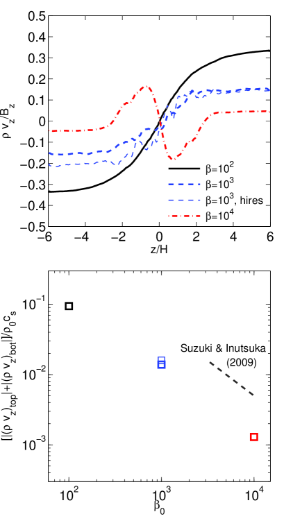
In the bottom panel of Figure 9, we show the total mass outflow rate $\dot{M}_{w}$ measured from the two vertical boundaries for all our simulations, with the numbers given in Table 2. We see that $\dot{m}_{w}$ scales roughly linearly with $1/\beta_{0}$, which is consistent with Suzuki & Inutsuka (2009) and Suzuki et al. (2010), while extending the range of $\beta_{0}$ from $10^{4}$ in their case down to $10^{2}$. From the definition of the Alfvén point, the mass loss rate can be expressed as

$$\dot{m}_{w}=2\sqrt{\rho}\bigg{|}_{A}\cdot|B_{z}|\ ,$$ (24)

where $|_{A}$ denotes value at the Alfvén point. A linear scaling of $\dot{m}_{w}$ with $1/\beta_{0}$ indicates that $\rho\propto B_{z}^{2}\propto 1/\beta_{0}$ at the Alfvén point, which is in line with the fact that the location of the Alfvén points decreases in height as net vertical field increases (the change in density profile due to magnetic pressure support is not as significant). Moreover, based on the same scaling, $v_{z}$ at the Alfvén point is expected to be constant, which is roughly the case as seen from Figure 8.

4.2.1 Determining $\dot{m}_{w}$

In Figure 9, we also indicate the scaling relation of $\dot{m}_{w}$ with $\beta_{0}$ from Suzuki & Inutsuka (2009). We find that while our measured $\dot{m}_{w}$ follows the same trend, while our proportional coefficient is about a factor of $5$ smaller than theirs. Besides that our vertical box size is slightly larger ($12H$ versus $8\sqrt{2}\approx 11.3H$), this difference is mainly due to the different outflow boundary conditions implemented in our simulations from theirs. In fact, the rate of mass outflow $\dot{m}_{w}$ is not a well determined quantity in local shearing-box type simulations because of the additional degree of freedom. Moreover, in both Fromang et al. (2012) and Lesur et al. (2012), it was found that $\dot{m}_{w}$ decreases as the vertical size of the simulation box increases, which again suggests that $\dot{m}_{w}$ can not be reliably obtained from shearing-box simulations.

Figure 11.— Same as Figure 7, but for run B4 only, and color represents the horizontally averaged radial magnetic field.

Since the vertical gravity increases linearly with $z$ in shearing-box approximation, the gas has to overcome stronger and stronger potential well in order to flow out as box height increases. In reality, the vertical increases only as $z/(R^{2}+z^{2})^{3/2}$, where $R$ is the distance to the central object, hence shearing-box approximation fails at $z\gtrsim R$. Fromang et al. (2012) considered higher order expansion of the real potential which would also require the radial potential to be modified to the same order. They noticed that this procedure would introduce curvature and no longer fit into the shearing-box framework.

The mass loss rate in real systems should be a well defined quantity, and we speculate that it should be comparable to the mass loss rate in shearing-box simulations performed with box size $L_{z}\approx 2R$. Suppose the mass outflow rate scales as

$$\frac{\dot{m}_{w}}{2\rho_{0}c_{s}}=\frac{A}{(L_{z}/H)^{\nu}}\frac{B_{0}^{2}}{2P_{0}}\ ,$$ (25)

where $A$ is a dimensionless constant, the index $\nu$ describes the scaling of $\dot{m}_{w}$ on the box height, and we have assumed that $\dot{m}_{w}\propto 1/\beta_{0}$ as suggested by the simulations discussed in the previous subsection, with $B_{0}$ denoting the background vertical field strength. With a little algebra, we find

$$\dot{m}_{w}=\frac{AB_{0}^{2}}{L_{z}\Omega}\bigg{(}\frac{L_{z}}{H}\bigg{)}^{1-\nu}\ .$$ (26)

In particular, if $\nu\approx 1$ (S. Fromang, 2011, private communication), then our hypothesis ($L_{z}=2R$) yields $\dot{m}_{w}\approx AB_{0}^{2}/2R\Omega$. This means that the mass loss rate can be found once the coefficient $A$ is known. Moreover, $\dot{m}_{w}$ is solely determined by the background vertical field strength and does not depend on the disk thickness or the disk surface density. On the other hand, if $\nu$ deviates from $1$, then one would expect $\dot{m}_{w}\propto(H/R)^{\nu-1}$.

In sum, although $\dot{m}_{w}$ is not well determined from shearing-box simulations, we argue that by carefully studying the dependence of $\dot{m}_{w}$ on the height of the simulation box, it is possible to obtain a physical estimate of the mass loss rate.

4.2.2 Evolutionary Scenarios

While we have demonstrated the correlation $\dot{m}_{w}\propto 1/\beta_{0}$, we have not discussed the range that it is applicable. Reading from Table 6, we see that $\dot{m}_{w}$ for $\beta_{0}=100$ is somewhat smaller than the expected linear correlation, which is suggestive of saturation. Indeed, the rate of mass outflow measured in Lesur et al. (2012) for a similar numerical setup (their run 1Dz6) with $\beta_{0}\sim 10$ gives $\dot{m}_{w}=0.234$ (multiplied by 2 to account for two surfaces), which is only a factor of 2.5 times higher than our case with $\beta_{0}=100$ ($\dot{m}_{w}=0.0944$). With further stronger magnetic field that is too strong for the MRI to operate, Ogilvie (2012) showed that the rate of mass outflow should rapidly decrease once $\beta_{0}$ drops below $1$. Therefore, the scaling relation $\dot{m}_{w}\propto 1/\beta_{0}$ holds up to $\beta_{0}\gtrsim 100$, beyond which the mass loss rate slows down and will eventually fall off rapidly for strong super-equipartition field field.

These results, all together, suggest an evolutionary scenario. Assuming no magnetic flux evolution, the disk would lose mass at constant rate (assuming $\nu=1$) until the midplane net vertical field exceeds equipartition. Lesur et al. (2012) explored such a scenario in their 1D simulations and confirmed the steady decrease of mass loss rate with increasing magnetization in the strong field regime. A strongly magnetized thin accretion disk may gradually evolve into such a stage, where the rate of mass loss is self-regulated so that it loses mass faster as more mass is fed into the disk (increasing $\beta_{0}$, but still $\beta_{0}<1$), while loses mass slower if the mass loss is not compensated (decreasing $\beta_{0}$). The disk structure would be similar to a jet-emitting disk (Combet & Ferreira, 2008), which is tenuous with super equipartition field. Alternatively, if the evolution starts from a strongly magnetized thick disk, the mass loss rate can be so large that the disk will be depleted in a few orbits. For example, without feeding mass to our run B2, the mass loss time scale is only about 5 orbits. Such rapid mass loss may lead to catastrophic disruption of the disk, such as in core-collapse supernovae where rapidly rotating progenitor core is threaded by extremely strong magnetic fields (Burrows et al., 2007).

4.3. Fate of the Outflow

In this subsection we discuss whether the outflow launched from shearing-box MRI simulations can be connected to a global Blandford-Payne type disk wind. The key to this question lies in the symmetry. We note that due to the neglect of curvature, shearing-box approximation does not specify which side of the radial domain the central object is located. For a physical disk wind, symmetry requires that the outflow from the top and bottom sides of the disk should be inclined towards the same radial and azimuthal directions (which would be considered as radially outward and trailing), and remains so at all times. Since gas flows along magnetic field lines, the mean magnetic field at the top and bottom sides of the disk should be bent to the same direction.

The first difficulty for outflow-wind connection is the magnetic dynamo, applicable to the cases with $\beta_{0}\gtrsim 10^{3}$ as we discussed in Secion 3.3. The constant flipping of the mean azimuthal (as well as radial, see Figure 11) field lines means that the direction of the outflow would constantly swap between radially inward and outward, either of the directions would be invalid for a global disk wind. Although our simulations with $\beta_{0}=10^{4}$ are in many aspects very similar to simulations by Suzuki & Inutsuka (2009), Suzuki et al. (2010), and Fromang et al. (2012), they argue that such phenomenon leads to the time variability of the wind. However, we stress here that the simple fact of cyclic sign change of the large-scale field is already inconsistent with global wind geometry.

Figure 12.— Time-averaged vertical profiles of magnetic field (left) and velocity (right) for run B2 with $\beta_{0}=100$. All in code units.

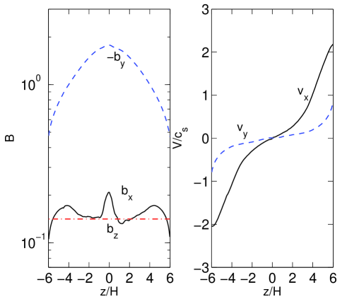
The second difficulty is that even there were no dynamo, such as the case for $\beta_{0}=10^{2}$, the natural symmetry from the simulation is unphysical for it to be connected to a global disk wind. In Figure 12, we show the vertical profiles of the magnetic field and velocity fields for run B2. Clearly, the outflows at the top and bottom sides of the disk are inclined toward opposite directions, which is inconsistent with a global disk wind. Even in the presence of the dynamo, there is a good chance that field lines at the top and bottom sides tend to incline toward different directions (as can be tracked in Figures 7 and 11).

Symmetry is also directly related to the vertical angular momentum transport by the outflow, as we discussed in Section 3.2. With the wrong symmetry, the wind stress (10) at the top and bottom sides of the disk have the same sign, and cancel each other, hence the net vertical angular momentum transport vanishes.

One might attribute this “wrong-symmetry” problem to the one extra degree of freedom in shearing-box simulations, which could possibly be avoided by performing global simulations. While it is certainly important to explore the same problem in global geometry, it has been suggested by Ogilvie (2012) that global effects can be effectively taken into account by applying some additional constraints on the vertical boundaries. Ogilvie constructed a 1D model for launching disk wind / jet in the shearing-box approximation, where a much stronger net vertical field $\beta_{0}\leq 1$ was assumed so as to suppress the MRI. He assigned the two free parameters at the vertical boundaries to be the strength of the radial and azimuthal magnetic fields (he has two parameters because the Alfvén point turns out to be beyond his computational domain), and was able to successfully construct laminar wind solutions with the desired symmetry for the given constraints.

In view of this possibility, we further modify our vertical boundary conditions so that the mean radial (or azimuthal) magnetic field in the last four grid zones at the vertical boundary are set to some fixed value, which is done by first calculating the mean radial (or azimuthal) field in these zones, and then subtracting a constant radial (or azimuthal) field uniformly in all these cells to make the mean field equal to the desired value without violating the divergence-free condition. As we see in Figure 12, the mean radial field at vertical boundaries is roughly the same as the mean vertical field in strength. Therefore, we demand that the field incline by $45^{\circ}$ at vertical boundaries in the $\hat{x}-\hat{z}$ plane, and require that the mean radial fields at the two vertical boundaries have opposite signs which conforms to the desired symmetry. However, after performing various experiments on smaller domain test runs with parameters similar to runs B2, B3 and B4, we find that such a treatment does not have an evident physical effect on the profile of the mean flow and mean field, except for introducing a strong current sheet at the vertical boundaries. This fact has also been discussed in Lesur et al. (2012), and we conclude that the poloidal field inclination at disk surface, particularly the symmetry of the mean horizontal fields, is insensitive to the imposed vertical boundary condition the once the Alfvén point is contained within the simulation domain.

In sum, we conclude that whether or not the MRI turbulence is accompanied by dynamo activities, the outflow from the shearing-box MRI simulations is unlikely to be directly connected to a global disk wind. The fate of the outflow remains to be explored using global simulations.

5. Discussion and Conclusions

5.1. Summary

In this paper, we have successfully performed local stratified shearing-box simulations of the MRI that include a strong vertical magnetic flux with midplane plasma $\beta$ of the net vertical field ranging from $\beta_{0}=10^{4}$ to $10^{2}$, a regime that has not been explored while is very likely relevant to accretion disks in many astrophysical systems. Such a magnetic configuration gives rise to very vigorous MRI turbulence, and simultaneously launches an outflow. We studied the properties of the MRI turbulence as well as the disk outflow in detail and our major findings are summarized below.

For the properties of the MRI turbulence, we find

• With relatively weak net vertical field of $\beta_{0}\gtrsim 10^{3}$, the disk consists of a gas pressure dominated disk midplane and a magnetic dominated disk corona ($\beta\sim 0.1-1$). By contrast, the entire disk becomes magnetically dominated when $\beta_{0}\lesssim 10^{3}$. The strong magnetic support substantially modifies the vertical structure of the disk and makes it substantially thicker.

• Turbulent magnetic and kinetic energies increase monotonically with net vertical magnetic flux, and saturate when $\beta_{0}\lesssim 10^{3}$. The MRI also generates large scale toroidal magnetic field whose strength increases monotonically with net vertical field, and dominates the total magnetic energy over contribution from turbulence for $\beta\lesssim 10^{3}$.

• The Shakura-Sunyaev parameter $\alpha$ increases monotonically with net vertical magnetic flux, ranging from $\alpha\sim 0.08$ at $\beta_{0}=10^{4}$ to $\alpha\gtrsim 1.0$ for $\beta=10^{2}$. Maxwell stress dominates Reynolds stress by a factor of 4-7. For weak net vertical flux of $\beta_{0}\gtrsim 10^{3}$, turbulent fluctuations dominates the contribution to $\alpha$, while for $\beta_{0}\lesssim 10^{3}$, radial transport of angular momentum is dominated by the large scale fields.

• The MRI dynamo that generates cyclic flips of the mean toroidal field persists in the presence of weak net vertical magnetic flux, but becomes more sporadic with less periodicity as net flux increases. The dynamo is completely suppressed when the net flux is strong with $\beta_{0}<10^{3}$, where the mean toroidal field exceeds equipartition strength and never flips.

Our results demonstrate the crucial dependence of the behavior of the MRI turbulence on the net vertical magnetic flux. In particular, there is a critical net vertical magnetic flux of $\beta_{0}\approx 10^{3}$ near which many aspects of the MRI turbulence change qualitatively. Additionally, more careful convergence study is still needed, and deeper understanding about the properties with MRI turbulence would further benefit from the study of Prantl number dependence (Fromang et al., 2007; Longaretti & Lesur, 2010; Fromang et al., 2012).

For the properties of the disk outflow, we find

• The slow magnetosonic point and the Alfvén point are always contained in our simulation box. The location of these critical points shifts towards the disk midplane as net vertical magnetic flux increases. The launching and acceleration of the outflow are due to the magnetocentrifugal mechanism, where surface magnetic field is sufficiently inclined.

• There is a robust trend that the outflow mass loss rate $\dot{m}_{w}$ increases with increasing net vertical field, and tends saturate at $\beta_{0}\lesssim 10^{2}$. Although $\dot{m}_{w}$ can not be well determined from shearing-box simulations, its exact value in real systems is likely to be much smaller than the measured from local simulations and may depend on the aspect ratio $H/R$.

• The outflow from the MRI simulations is unlikely to be directly connected to a global disk wind for geometric reasons. For $\beta_{0}\gtrsim 10^{3}$, the large scale radial and azimuthal field lines are constantly flipped due to the dynamo activities without a permanent bending direction. For $\beta_{0}\lesssim 10^{3}$, the large scale magnetic fields do not change sign across the midplane, hence the field lines at the two sides of the disk bend to opposite directions, inconsistent with a global wind geometry.

• Angular momentum transport by the disk outflow is likely to play a minor role compared with that by the MRI turbulence for relatively weak net vertical magnetic flux. With stronger net vertical flux ($\beta_{0}\lesssim 10^{3}$), the symmetry of the flow (as the dynamo is suppressed) makes net vertical angular momentum transport be zero, but gives oppositely directed inflow/outflow with substantial mass flux.

It has been reported that $\dot{m}_{w}$ from shearing-box MRI simulations decreases with increasing height of the simulation domain, which is related to the intrinsic limitations of the shearing-box framework. We propose that a careful study of the height dependence can help determining the true value of $\dot{m}_{w}$ in real systems. Our results leave an open question on the fate of the outflow, which can only be reliably explored using global simulations and will be discussed further in Section 5.3.

5.2. Implications for Global Disk Evolution

We note that shearing-box simulations with zero net vertical flux tend to give $\alpha\sim 0.01-0.02$ with confirmed numerical convergence (Miller & Stone, 2000; Hirose et al., 2006; Shi et al., 2010; Davis et al., 2010; Simon et al., 2012). The vast dominance of simulations of this type has, to some extent, implicitly created a misconception that the $\alpha$ value resulting from the MRI turbulence if of the order $0.01$. On the observational side, the value of $\alpha$ can be estimated from the viscous timescale of transient systems such as dwarf novae, X-ray transient and FU Ori bursts, where it was found to be of the order $0.1$ or larger (Smak, 1999; Dubus et al., 2001; Zhu et al., 2007). Such apparent discrepancy leads King et al. (2007) to question about the efficiency of the MRI in driving disk accretion and evolution. The dependence of $\alpha$ on net vertical magnetic flux has already been extensively discussed in unstratified shearing-box simulations (Hawley et al., 1995; Sano et al., 2004; Pessah et al., 2007; Longaretti & Lesur, 2010). Our simulations further confirm and quantify this trend using more realistic simulations with vertical stratification, and demonstrate that the above discrepancy can be naturally resolved if accretion disks are threaded by some large scale poloidal magnetic fields.

The strong dependence of $\alpha$ on $\beta_{0}$ immediately indicates that the evolution of accretion disks strongly depends on the distribution of poloidal magnetic flux through the disk. On the other hand, because of flux freezing in ideal MHD, the distribution of magnetic flux is intimately connected to disk evolution (as well as turbulent diffusion and reconnection due to the MRI). Therefore, the mutual dependence of disk evolution and magnetic flux evolution makes the problem of disk accretion intrinsically non-local, hence a full understanding of accretion disk structure and evolution requires global simulations.

Most global simulations to date adopt a magnetic field geometry that is analogous to zero net-flux shearing-box: the simulations are initialized either with single/multiple poloidal magnetic loops for a thick disk torus (Hawley, 2000; De Villiers et al., 2003; Penna et al., 2010), or with pure toroidal magnetic field in a thin power-law disk (Fromang & Nelson, 2006; Beckwith et al., 2011; Flock et al., 2011). These simulations generally show values of $\alpha$ that are slightly higher than $0.01$ ($\sim 0.025$). In these simulations, the MRI generates net vertical magnetic flux in the local patches of the disk connected by coronal loops and the local stress correlates with the net vertical flux (Tout & Pringle, 1992; Sorathia et al., 2010). Combined with our study, the local net vertical flux in these global simulations is sufficient to account for the slightly higher total stress $\alpha$ than that in zero net flux shearing-box simulations. However, the distribution of local net vertical magnetic flux falls off quickly with stronger net flux, hence the total value of $\alpha$ can not be enhanced substantially.

Initial magnetic field geometry plays an important role in global simulations of the MRI, although the situation with large scale poloidal fields threading the disk have rarely been explored. Semi-analytical treatment reveals that the global distribution of large-scale magnetic flux in accretion disks depends largely on the ratio of turbulent viscosity and resistivity (Lubow et al., 1994a), as well as the vertical structure of the disk (Guilet & Ogilvie, 2012). Together with these works, our simulations provide strong motivation for exploring the consequence of large scale poloidal field in global simulations. Such simulations will not only expand our knowledge the MRI, but will also address the fate of the outflow, which we discuss in the next section.

5.3. Disk Wind Launching in Global Simulations?

It has been recognized that strong net vertical field that approaches equipartition strength at the disk midplane is necessary for launching a steady-state wind (Wardle & Koenigl, 1993; Ferreira & Pelletier, 1995; Ogilvie & Livio, 2001). The requirement may be relaxed to lower magnetizations (Murphy et al., 2010), while for magnetization that is too low the outflow is either suppressed or highly unsteady (Tzeferacos et al., 2009). Numerous global simulations have studied launching of disk wind in the context of protostellar disks (e.g., Kato et al., 2002; Casse & Keppens, 2002; Zanni et al., 2007)). However, as noted in Section 1, the use of artificial diffusion in these simulations do not properly reflect the disk microphysics. For strong net vertical field that would suppress the MRI, the artificial diffusion has unknown origin (and the non-ideal MHD effects can not be properly treated as artificial diffusion, Bai & Stone, 2012). For weaker net vertical field, the MRI is the presumed source of artificial diffusion. However, our evidence against direct wind launching all originate from the microphysical effects of the MRI (such as the MRI dynamo) that can not be captured in these simulations.

Another family of global simulations focus on non-radiative accretion disks around black holes (BH). These simulations either use psudo-Newtonian gravitational potential for the BH or adopt a general-relativistic prescription. Despite the non-Keplerian nature in the vicinity of the BHs, the physics of the MRI that is not too close to the innermost stable orbit is similar. Most of these simulations adopt similar poloidal loop field geometry and focus on jet launching which deals with the innermost part of the accretion flow, a few of them do have included large scale poloidal fields. In particular, Beckwith et al. (2009) initialized the simulations with pure vertical magnetic fields with $\beta_{0}\sim 10^{2}$. However, upon saturation the launching of a Blandford-Payne type wind was not observed, which was attributed to a global “coronal mechanism” that governs the magnetic flux evolution. Also, their simulations have relatively small radial domain and very thick disk. Significant outflow has been reported in two-dimensional MHD simulations (Stone & Pringle, 2001; Yuan et al., 2012), where MRI is a transient phenomenon. More recently, Tchekhovskoy et al. (2011), McKinney et al. (2012) and Narayan et al. (2012) studied the accretion flow with large scale initial poloidal field in the inner disk with $\beta_{0}\sim 10^{2}$ which leads to a “magnetically arrested” or “magnetically chocked” accretion flow due to the accumulation of magnetic flux in the vicinity of the BH. The MRI in the main disk was properly resolved in these simulations, however, they do not report any significant disk outflow in the inner region of the disks, and found that the jet power is directly correlated with BH spin.

Together, it appears that Blandford-Payne type disk wind has not been unambiguously identified in global simulations with properly resolved MRI turbulence. Future studies should focus on the largely unexplored area of 3D global simulations for thin accretion disks in the presence of large-scale poloidal magnetic field. Large simulation domain in both radius and polar angle, fine resolution in the disk, and careful treatment of boundary conditions are required (T. Suzuki, private communication), and such simulations are essential to ascertain the nature of the outflow, and to reveal the underlying physics governing the evolution of accretion disks.

References

- Bai & Stone (2011) Bai, X.-N. & Stone, J. M. 2011, ApJ, 736, 144
- Bai & Stone (2012) —. 2013, submitted to ApJ, arXiv:1301.0318
- Balbus & Hawley (1991) Balbus, S. A. & Hawley, J. F. 1991, ApJ, 376, 214
- Beckwith et al. (2011) Beckwith, K., Armitage, P. J., & Simon, J. B. 2011, MNRAS, 416, 361
- Beckwith et al. (2009) Beckwith, K., Hawley, J. F., & Krolik, J. H. 2009, ApJ, 707, 428
- Begelman et al. (1984) Begelman, M. C., Blandford, R. D., & Rees, M. J. 1984, Reviews of Modern Physics, 56, 255
- Blaes et al. (2007) Blaes, O., Hirose, S., & Krolik, J. H. 2007, ApJ, 664, 1057
- Blandford & Payne (1982) Blandford, R. D. & Payne, D. G. 1982, MNRAS, 199, 883
- Brandenburg et al. (1995) Brandenburg, A., Nordlund, A., Stein, R. F., & Torkelsson, U. 1995, ApJ, 446, 741
- Burrows et al. (2007) Burrows, A., Dessart, L., Livne, E., Ott, C. D., & Murphy, J. 2007, ApJ, 664, 416
- Cabrit (2007) Cabrit, S. 2007, in Lecture Notes in Physics, Berlin Springer Verlag, Vol. 723, Lecture Notes in Physics, Berlin Springer Verlag, ed. J. Ferreira, C. Dougados, & E. Whelan, 21
- Cao & Spruit (2002) Cao, X. & Spruit, H. C. 2002, A&A, 385, 289
- Casse & Keppens (2002) Casse, F. & Keppens, R. 2002, ApJ, 581, 988
- Combet & Ferreira (2008) Combet, C. & Ferreira, J. 2008, A&A, 479, 481
- Davis et al. (2010) Davis, S. W., Stone, J. M., & Pessah, M. E. 2010, ApJ, 713, 52
- De Villiers et al. (2003) De Villiers, J.-P., Hawley, J. F., & Krolik, J. H. 2003, ApJ, 599, 1238
- Dubus et al. (2001) Dubus, G., Hameury, J.-M., & Lasota, J.-P. 2001, A&A, 373, 251
- Fender (2006) Fender, R. 2006, Jets from X-ray binaries, ed. W. H. G. Lewin & M. van der Klis, 381–419
- Ferreira & Pelletier (1995) Ferreira, J. & Pelletier, G. 1995, A&A, 295, 807
- Flaig et al. (2010) Flaig, M., Kley, W., & Kissmann, R. 2010, MNRAS, 409, 1297
- Flock et al. (2011) Flock, M., Dzyurkevich, N., Klahr, H., Turner, N. J., & Henning, T. 2011, ApJ, 735, 122
- Fromang et al. (2012) Fromang, S., Latter, H. N., Lesur, G., & Ogilvie, G. I. 2012, A&A, submitted, arXiv:1210.6664
- Fromang & Nelson (2006) Fromang, S. & Nelson, R. P. 2006, A&A, 457, 343
- Fromang & Papaloizou (2007) Fromang, S. & Papaloizou, J. 2007, A&A, 476, 1113
- Fromang et al. (2007) Fromang, S., Papaloizou, J., Lesur, G., & Heinemann, T. 2007, A&A, 476, 1123
- Gaburov et al. (2012) Gaburov, E., Johansen, A., & Levin, Y. 2012, ApJ, 758, 103
- Goldreich & Lynden-Bell (1965) Goldreich, P. & Lynden-Bell, D. 1965, MNRAS, 130, 125
- Goodman & Xu (1994) Goodman, J. & Xu, G. 1994, ApJ, 432, 213
- Gressel (2010) Gressel, O. 2010, MNRAS, 405, 41
- Guan & Gammie (2011) Guan, X. & Gammie, C. F. 2011, ApJ, 728, 130
- Guan et al. (2009) Guan, X., Gammie, C. F., Simon, J. B., & Johnson, B. M. 2009, ApJ, 694, 1010
- Guilet & Ogilvie (2012) Guilet, J., & Ogilvie, G. I. 2012, MNRAS, 424, 2097
- Harris & Krawczynski (2006) Harris, D. E. & Krawczynski, H. 2006, ARA&A, 44, 463
- Hawley (2000) Hawley, J. F. 2000, ApJ, 528, 462
- Hawley (2001) —. 2001, ApJ, 554, 534
- Hawley et al. (1995) Hawley, J. F., Gammie, C. F., & Balbus, S. A. 1995, ApJ, 440, 742
- Hawley et al. (1996) —. 1996, ApJ, 464, 690
- Hawley et al. (2011) Hawley, J. F., Guan, X., & Krolik, J. H. 2011, ApJ, 738, 84
- Heinemann & Papaloizou (2009) Heinemann, T. & Papaloizou, J. C. B. 2009, MNRAS, 397, 64
- Hirose et al. (2006) Hirose, S., Krolik, J. H., & Stone, J. M. 2006, ApJ, 640, 901
- Johansen & Levin (2008) Johansen, A. & Levin, Y. 2008, A&A, 490, 501
- Johansen et al. (2009) Johansen, A., Youdin, A., & Klahr, H. 2009, ApJ, 697, 1269
- Kato et al. (2002) Kato, S. X., Kudoh, T., & Shibata, K. 2002, ApJ, 565, 1035
- King et al. (2007) King, A. R., Pringle, J. E., & Livio, M. 2007, MNRAS, 376, 1740
- Krasnopolsky et al. (1999) Krasnopolsky, R., Li, Z.-Y., & Blandford, R. 1999, ApJ, 526, 631
- Latter et al. (2010) Latter, H. N., Fromang, S., & Gressel, O. 2010, MNRAS, 406, 848
- Latter et al. (2009) Latter, H. N., Lesaffre, P., & Balbus, S. A. 2009, MNRAS, 394, 715
- Lesur et al. (2012) Lesur, G., Ferreira, J., & Ogilvie, G. I. 2013, A&A, 550, A61
- Lesur & Longaretti (2007) Lesur, G. & Longaretti, P. 2007, MNRAS, 378, 1471
- Lesur & Ogilvie (2008) Lesur, G. & Ogilvie, G. I. 2008, A&A, 488, 451
- Li (1995) Li, Z.-Y. 1995, ApJ, 444, 848
- Longaretti & Lesur (2010) Longaretti, P. & Lesur, G. 2010, A&A, 516, A51+
- Lubow et al. (1994a) Lubow, S. H., Papaloizou, J. C. B., & Pringle, J. E. 1994a, MNRAS, 267, 235
- Lubow et al. (1994b) Lubow, S. H., Papaloizou, J. C. B., & Pringle, J. E. 1994b, MNRAS, 268, 1010
- McKinney et al. (2012) McKinney, J. C., Tchekhovskoy, A., & Blandford, R. D. 2012, MNRAS, 423, 3083
- Miller & Stone (2000) Miller, K. A. & Stone, J. M. 2000, ApJ, 534, 398
- Mirabel & Rodríguez (1999) Mirabel, I. F. & Rodríguez, L. F. 1999, ARA&A, 37, 409
- Moll (2012) Moll, R. 2012, A&A, 548, A76
- Murphy et al. (2010) Murphy, G. C., Ferreira, J., & Zanni, C. 2010, A&A, 512, A82
- Narayan et al. (2012) Narayan, R., Sadowski, A., Penna, R. F., & Kulkarni, A. K. 2012, MNRAS, 426, 3241
- Newcomb (1961) Newcomb, W. A. 1961, Physics of Fluids, 4, 391
- Ogilvie (2012) Ogilvie, G. I. 2012, MNRAS, 423, 1318
- Ogilvie & Livio (2001) Ogilvie, G. I. & Livio, M. 2001, ApJ, 553, 158
- Ouyed & Pudritz (1997) Ouyed, R. & Pudritz, R. E. 1997, ApJ, 482, 712
- Parker (1966) Parker, E. N. 1966, ApJ, 145, 811
- Pelletier & Pudritz (1992) Pelletier, G. & Pudritz, R. E. 1992, ApJ, 394, 117
- Penna et al. (2010) Penna, R. F., McKinney, J. C., Narayan, R., Tchekhovskoy, A., Shafee, R., & McClintock, J. E. 2010, MNRAS, 408, 752
- Pessah et al. (2007) Pessah, M. E., Chan, C.-k., & Psaltis, D. 2007, ApJ, 668, L51
- Pessah & Goodman (2009) Pessah, M. E. & Goodman, J. 2009, ApJ, 698, L72
- Pessah & Psaltis (2005) Pessah, M. E., & Psaltis, D. 2005, ApJ, 628, 879
- Pudritz & Norman (1983) Pudritz, R. E. & Norman, C. A. 1983, ApJ, 274, 677
- Reipurth & Bally (2001) Reipurth, B. & Bally, J. 2001, ARA&A, 39, 403
- Sano et al. (2004) Sano, T., Inutsuka, S.-i., Turner, N. J., & Stone, J. M. 2004, ApJ, 605, 321
- Shakura & Sunyaev (1973) Shakura, N. I. & Sunyaev, R. A. 1973, A&A, 24, 337
- Shi et al. (2010) Shi, J., Krolik, J. H., & Hirose, S. 2010, ApJ, 708, 1716
- Simon et al. (2012) Simon, J. B., Beckwith, K., & Armitage, P. J. 2012, MNRAS, 422, 2685
- Simon et al. (2011) Simon, J. B., Hawley, J. F., & Beckwith, K. 2011, ApJ, 730, 94
- Smak (1999) Smak, J. 1999, Acta Astron., 49, 391
- Sorathia et al. (2010) Sorathia, K. A., Reynolds, C. S., & Armitage, P. J. 2010, ApJ, 712, 1241
- Stone & Gardiner (2010) Stone, J. M. & Gardiner, T. A. 2010, ApJS, 189, 142
- Stone et al. (2008) Stone, J. M., Gardiner, T. A., Teuben, P., Hawley, J. F., & Simon, J. B. 2008, ApJS, 178, 137
- Stone et al. (1996) Stone, J. M., Hawley, J. F., Gammie, C. F., & Balbus, S. A. 1996, ApJ, 463, 656
- Stone & Pringle (2001) Stone, J. M. & Pringle, J. E. 2001, MNRAS, 322, 461
- Suzuki & Inutsuka (2009) Suzuki, T. K. & Inutsuka, S.-i. 2009, ApJ, 691, L49
- Suzuki et al. (2010) Suzuki, T. K., Muto, T., & Inutsuka, S.-i. 2010, ApJ, 718, 1289
- Tchekhovskoy et al. (2011) Tchekhovskoy, A., Narayan, R., & McKinney, J. C. 2011, MNRAS, 418, L79
- Tout & Pringle (1992) Tout, C. A. & Pringle, J. E. 1992, MNRAS, 259, 604
- Tzeferacos et al. (2009) Tzeferacos, P., Ferrari, A., Mignone, A., Zanni, C., Bodo, G., & Massaglia, S. 2009, MNRAS, 400, 820
- Uzdensky (2012) Uzdensky, D. A. 2012, arXiv:1205.6537
- Vishniac & Brandenburg (1997) Vishniac, E. T. & Brandenburg, A. 1997, ApJ, 475, 263
- Wardle & Koenigl (1993) Wardle, M. & Koenigl, A. 1993, ApJ, 410, 218
- Yousef et al. (2008) Yousef, T. A., Heinemann, T., Schekochihin, A. A., Kleeorin, N., Rogachevskii, I., Iskakov, A. B., Cowley, S. C., & McWilliams, J. C. 2008, Physical Review Letters, 100, 184501
- Yuan et al. (2012) Yuan, F., Bu, D., & Wu, M. 2012, ApJ, 761, 130
- Zanni et al. (2007) Zanni, C., Ferrari, A., Rosner, R., Bodo, G., & Massaglia, S. 2007, A&A, 469, 811
- Zhu et al. (2007) Zhu, Z., Hartmann, L., Calvet, N., Hernandez, J., Muzerolle, J., & Tannirkulam, A.-K. 2007, ApJ, 669, 483
- Ziegler & Rüdiger (2000) Ziegler, U. & Rüdiger, G. 2000, A&A, 356, 1141