Towards a Monge-Kantorovich metric
in noncommutative geometry

Abstract

We investigate whether the identification between Connes’ spectral distance in noncommutative geometry and the Monge-Kantorovich distance of order $1$ in the theory of optimal transport - that has been pointed out by Rieffel in the commutative case - still makes sense in a noncommutative framework. To this aim, given a spectral triple $({\mathcal{A}},{\mathcal{H}},D)$ with noncommutative ${\mathcal{A}}$, we introduce a “Monge-Kantorovich”-like distance $W_{D}$ on the space of states of ${\mathcal{A}}$, taking as a cost function the spectral distance $d_{D}$ between pure states. We show in full generality that $d_{D}\leq W_{D}$, and exhibit several examples where the equality actually holds true, in particular on the unit two-ball viewed as the state space of $M_{2}({\mathbb{C}})$. We also discuss $W_{D}$ in a two-sheet model (product of a manifold by ${\mathbb{C}}^{2}$), pointing towards a possible interpretation of the Higgs field as a cost function that does not vanish on the diagonal.

I Introduction

In [6] Connes noticed that the geodesic distance on a compact Riemannian manifold ${\mathcal{M}}$ (connected and without boundary) can be retrieved in purely algebraic terms, from the knowledge of both the algebra $C^{\infty}({\mathcal{M}})$ of smooth functions on ${\mathcal{M}}$ and the signature (or Hodge-Dirac operator) $d+d^{\dagger}$, where $d$ is the exterior derivative. Explicitly, one has

$$d_{\text{geo}}(x,y)=\sup_{f\in C^{\infty}({\mathcal{M}})}\left\{\lvert\delta_{x}(f)-\delta_{y}(f)\rvert,\;\left\lVert[d+d^{\dagger},\pi(f)]\right\rVert\leq 1\right\}\vspace{-.35truecm}$$ (1.1)

where

• $\pi$ denotes the representation of the commutative algebra $C^{\infty}({\mathcal{M}})$ by multiplication on the Hilbert space $\Omega^{\bullet}({\mathcal{M}})$ of square integrable differential forms on ${\mathcal{M}}$;

• the norm of the commutator is the operator norm on ${\mathcal{B}}(\Omega^{\bullet}({\mathcal{M}}))$ (bounded operators on $\Omega^{\bullet}({\mathcal{M}})$):

  $$\left\lVert A\right\rVert=\sup_{\left\lVert\psi\right\rVert_{\Omega}=1}\left\lVert A\psi\right\rVert_{\Omega}$$ (1.2)

  for any $A\in{\mathcal{B}}(\Omega^{\bullet}({\mathcal{M}}))$, with $\left\lVert\cdot\right\rVert_{\Omega}$ the Hilbert space norm of $\Omega^{\bullet}({\mathcal{M}})$;

• $\delta_{x}:f\to f(x)$ is the evaluation at $x\in{\mathcal{M}}$.

Evaluations are nothing but the pure states of the $C^{*}$-closure $C({\mathcal{M}})$ of $C^{\infty}({\mathcal{M}})$. Recall that a state of a $C^{*}$-algebra ${\mathcal{A}}$ is a positive linear form on ${\mathcal{A}}$ with norm $1$. The space of states, denoted ${\cal S}({\mathcal{A}})$, is convex and its extremal points are called pure states. By Gelfand theorem, any commutative $C^{*}$-algebra ${\mathcal{A}}$ is isomorphic to the algebra of functions vanishing at infinity on its pure state space ${\cal P}({\mathcal{A}})$ and - conversely - any locally compact topological space ${\cal X}$ is homeomorphic to the pure state space of $C_{0}({\cal X})$,

$${\mathcal{A}}\simeq C_{0}({\cal P}({\mathcal{A}}))\quad{\cal X}\simeq{\mathcal{P}}(C_{0}({\cal X}).$$ (1.3)

In modern terms, the category of commutative $C^{*}$-algebras is (anti)-isomorphic to the category of locally compact topological spaces. The compact case corresponds to unital algebras.

With Gelfand theorem in minds, it is natural to extend (1.1) to non-pure states $\varphi,\tilde{\varphi}\in{\cal S}(C({\mathcal{M}}))$, defining

$$d_{d+d^{\dagger}}(\varphi,\tilde{\varphi})\doteq\sup_{f\in C^{\infty}({\mathcal{M}})}\left\{\lvert\varphi(f)-\tilde{\varphi}(f)\rvert,\;\left\lVert[d+d^{\dagger},\pi(f)]\right\rVert\leq 1\right\}.$$ (1.4)

Since the commutativity of the algebra $C^{\infty}({\mathcal{M}})$ does not enter (1.1), another natural extension is to the noncommutative setting. Namely, given a noncommutative algebra ${\mathcal{A}}$ acting by $\pi$ on some Hilbert space ${\mathcal{H}}$, together with an operator $D$ on ${\mathcal{H}}$ such that $[D,\pi(a)]$ is bounded for any $a\in{\mathcal{A}}$, one defines [7] for any $\varphi,\tilde{\varphi}\in{\cal S}({\mathcal{A}})$

$$d_{D}(\varphi,\tilde{\varphi})\doteq\sup_{a\in{\mathcal{B}}_{D}({\mathcal{A}})}\lvert\varphi(a)-\tilde{\varphi}(a)\rvert,$$ (1.5)

where

$${\mathcal{B}}_{D}({\mathcal{A}})\doteq\left\{a\in{\mathcal{A}},\left\lVert[D,\pi(a)]\right\rVert\leq 1\right\}$$ (1.6)

denotes the $D$-Lipschitz ball of ${\mathcal{A}}$. It is easy to check that $d_{D}$ satisfies all the properties of a distance on ${\cal S}({\mathcal{A}})$ (see e.g. [15, p.35]), except it may be infinite. Following the terminology of [16], we call it the spectral distance, but depending on the authors it may be called Connes or the noncommutative distance. Notice that - as in the commutative case - when ${\mathcal{A}}$ is not a $C^{*}$-algebra we consider the states of its $C^{*}$-closure in the operator norm coming from the representation $\pi$.

Therefore the spectral distance (1.5) appears as a generalization to the noncommutative setting of the Riemannian geodesic distance. The latter is retrieved between pure states in the commutative case

$$d_{d+d^{\dagger}}(\delta_{x},\delta_{y})=d_{\text{geo}}(x,y).$$ (1.7)

For non-pure states (still in the commutative case), Rieffel seems to have been the first to notice in [18] that (1.4) was nothing but Kantorovich’s dual formulation of the minimal transport between probability measures, with cost function the geodesic distance. Indeed, the set of states of $C(M)\ni\varphi$ is in $1$-to-$1$ correspondence with the set of probability measures $\text{Prob}({\mathcal{M}})\ni\mu$ on ${\mathcal{M}}$,

$$\varphi(f)=\int_{\mathcal{M}}f\,\mathrm{d}\mu,$$ (1.8)

and it is not difficult to check (as recalled in section II) that

$$d_{d+d^{\dagger}}(\varphi,\tilde{\varphi})=W(\mu,\tilde{\mu})$$ (1.9)

where $W$ denotes the Monge-Kantorovich (or Wasserstein) distance of order one with cost $d_{\text{geo}}$. The same result holds on a locally compact manifold, as soon as it is complete [11].

In this contribution, we investigate how the identification of the spectral distance with the Monge-Kantorovich metric could still make sense in a noncommutative context. Namely, given a noncommutative algebra ${\mathcal{A}}$ acting on some Hilbert ${\mathcal{H}}$ together with an operator $D$ such that $[D,\pi(a)]$ is bounded for any $a\in{\mathcal{A}}$, is there some “optimal transport in noncommutative geometry” such that the associated Monge-Kantorovich distance coincides with the spectral distance (1.5) ? We provide a tentative answer, introducing on the state space ${\cal S}({\mathcal{A}})$ a new distance $W_{D}$, obtained by taking as a cost function the spectral distance $d_{D}$ on the pure state space ${\cal P}({\mathcal{A}})$. The main properties of this “Monge-Kantorovich”-like distance are worked out in proposition III.1: it is shown in full generality that $d_{D}\leq W_{D}$ on ${\cal S}({\mathcal{A}})$, with equality on ${\cal P}({\mathcal{A}})$ as well as between any non-pure states obtained as convex linear combinations of the same two pure states. In particular, this allows to show that $d_{D}=W_{D}$ on the two-ball, viewed as the space of states of ${\mathcal{A}}=M_{2}({\mathbb{C}})$.

We begin with the commutative case (section II), recalling in proposition II.1 why $d_{d+d^{\dagger}}$ coincides with the Monge-Kantorovich distance $W$. Then we investigate the noncommutative case and introduce the new distance $W_{D}$ in section III. Section IV deals with examples.

II The commutative case

II.1 Monge-Kantorovich and spectral distance

Recall that given two probability measures $\mu$, $\tilde{\mu}$ on a metric space $({\cal X},d)$ (non-necessarily compact), the Monge-Kantorovich distance is

$$W(\mu,\tilde{\mu})=\inf_{\pi}\int_{{\cal X}\times{\cal X}}\!\!\!\!\!\!\!\!\!\!\!\!\mathrm{d}\pi\quad d(x,y)$$ (2.1)

where the infimum is on all the measures on ${\cal X}\times{\cal X}$ whose marginals are $\mu$ and $\tilde{\mu}$. In his seminal work [13, 14], Kantorovich showed there exists a dual formulation,

$$W(\mu,\tilde{\mu})=\sup_{\left\lVert f\right\rVert_{\mathrm{Lip}}\leq 1,\,f\in L^{1}(\mu_{1})\cap L^{1}(\mu_{2})}\left(\int_{\cal X}f\mathrm{d}\mu-\int_{\cal X}f\mathrm{d}\tilde{\mu}\right)$$ (2.2)

for any pair of probability measures on ${\cal X}$ such that the right-hand side in the above expression is finite. The supremum is on all real $\mu,\tilde{\mu}$-integrable real functions $f$ that are 1-Lipschitz, that is to say

$$|f(x)-f(y)|\leq d(x,y)\quad\forall\;x,y\in{\cal X}.$$ (2.3)

Take now $({\cal X},d)$ a locally compact Riemannian manifold $({\mathcal{M}},d_{\text{geo}})$ and consider the spectral distance (1.4). The formula is the same as in the compact case, except that we want the algebra to be represented by bounded operators. So instead of $C^{\infty}({\mathcal{M}})$ we look for the supremum on the algebra $C^{\infty}_{0}({\mathcal{M}})$ of smooth functions vanishing at infinity. Let $\varphi,\tilde{\varphi}$ be two states of $C_{0}({\mathcal{M}})$ defined by probability measures $\mu,\tilde{\mu}$ via formula (1.8). That the Monge-Kantorovich distance $W(\mu,\tilde{\mu})$ equals the spectral distance $d_{d+d^{\dagger}}(\varphi,\tilde{\varphi})$ follows from the three well known points:

• the supremum in (1.5) can be equivalently searched on selfadjoint elements [12]. In the commutative case, this means we assume $f\in C_{0}^{\infty}({\mathcal{M}})$ is real.

• for real functions, the norm of the commutator $[d+d^{\dagger},\pi(f)]$, as an operator on $\Omega^{\bullet}({\mathcal{M}})$, is precisely the Lipschitz norm of $f$ (see [10] and also section II.3):

  $$\left\lVert f\right\rVert_{\text{Lip}}=\left\lVert[d+d^{\dagger},\pi(f)]\right\rVert.$$ (2.4)

• the supremum on $1$-Lipschitz smooth functions vanishing at infinity in the spectral distance formula is the same as the supremum on $1$-Lipschitz continuous functions non-necessarily vanishing at infinity in Monge-Kantorovich formula (for details cf e.g. [11, §2.2]).

Notice that for the last point to be true, it is important that ${\mathcal{M}}$ be complete. Under this condition one obtains

Proposition II.1

[18, 11] On a (connected, without boundary) complete Riemannian manifold ${\mathcal{M}}$, for any state $\varphi,\tilde{\varphi}\in S(C_{0}({\mathcal{M}}))$ one has

$$d_{d+d^{\dagger}}(\varphi,\tilde{\varphi})=W(\mu,\tilde{\mu}).$$ (2.5)

II.2 On the importance of being complete

It is not known to the author whether Kantorovich duality holds for non-complete manifolds (in the literature the completeness condition seems to be always assumed). In any case, (2.2) still makes sense as a definition of the Monge-Kantorovich distance for non-complete manifolds. The importance of the completeness condition is illustrated by simple examples, taken from [11].

Let ${\mathcal{M}}$ be a compact manifold and ${\cal N}={\mathcal{M}}\smallsetminus\left\{x_{0}\right\}.$ For example ${\mathcal{M}}=S^{1}=[0,1]$ and ${\cal N}=(0,1)$. The Monge-Kantorovich distance on $S^{1}$ is

$$W_{{\mathcal{M}}}(x,y)=\min\{|x-y|,1-|x-y|\},$$ (2.6)

which differs from $W_{{\cal N}}(x,y)=|x-y|$. On the contrary, for ${\mathcal{M}}=S^{2}$ and ${\cal N}=S^{2}\smallsetminus\left\{x_{0}\right\}$, one has $W_{\mathcal{M}}=W_{\cal N}$. Removing a point from a complete compact manifold may change or not the Monge-Kantorovich distance.

On the contrary, removing a point does not modify the spectral distance, in the sense that

$$d_{d+d^{\dagger}}^{{\mathcal{M}}}(\varphi_{1},\varphi_{2}) =\sup_{f\in C^{\infty}({\mathcal{M}})}\big{\{}|(\varphi_{1}-\varphi_{2})(f)|;\,||f||_{\mathrm{Lip}}\leq 1\big{\}}$$

$$=\sup_{f\in C^{\infty}({\mathcal{M}}),f(x_{0})=0}\big{\{}|(\varphi_{1}-\varphi_{2})(f)|;\,||f||_{\mathrm{Lip}}\leq 1\big{\}}$$

$$=\sup_{f\in C^{\infty}_{0}({\cal N})}\big{\{}|(\varphi_{1}-\varphi_{2})(f)|;\,||f||_{\mathrm{Lip}}\leq 1\big{\}}=d_{d+d^{\dagger}}^{{\cal N}}(\varphi_{1},\varphi_{2}).$$

Here we noticed that because $C^{\infty}({\mathcal{M}})$ has a unit ${\bf 1}$, if $f$ attains the supremum then so does $f-f(x_{0}){\bf 1}$ (the argument is still valid if the supremum is not attained, by considering a sequence of element in the Lipschitz ball tending to the infimum).

To summarize, the spectral and the Monge-Kantorovich distances are equal on the incomplete manifold $S^{2}\smallsetminus\left\{x_{0}\right\}$, but are not equal on $(0,1)$.

II.3 Spin, Laplacian and the Lipschitz ball

There exist alternative definitions of the Lipschitz ball (1.6). Instead of the signature operator $d+d^{\dagger}$, one can use as well the Dirac (or Atiyah) operator

$$\partial\!\!\!/=-i\sum_{\mu=1}^{\text{dim}{\mathcal{M}}}\gamma^{\mu}\partial_{\mu}.$$ (2.7)

Recall that the $\gamma^{\mu}$’s are selfadjoint matrices of dimension $M\leavevmode\nobreak\ \doteq\leavevmode\nobreak\ 2^{E(\frac{m}{2})}$, $m\doteq\text{dim}\,{\mathcal{M}}$, spanning an irreducible representation of the Clifford algebra. They satisfy

$$\gamma^{\mu}\gamma^{\nu}+\gamma^{\nu}\gamma^{\mu}=2g^{\mu\nu}{\mathbb{I}}_{M}.$$ (2.8)

With $\pi_{1}$ the multiplicative representation of $C_{0}({\mathcal{M}})$ on the Hilbert space ${\mathcal{H}}_{1}$ of square integrable spinors on ${\mathcal{M}}$,

$$\left(\pi_{1}(f)\psi\right)(x)=f(x)\psi(x)\quad\forall\psi\in{\mathcal{H}}_{1},\,x\in{\mathcal{M}},$$ (2.9)

one easily checks that $[\partial\!\!\!/,\pi_{1}(f)]$ acts as multiplication by $\sum_{\mu}\gamma^{\mu}\partial_{\mu}f$, since by the Leibniz rule

$$[\partial\!\!\!/,\pi_{1}(f)]\psi=\sum_{\mu}\gamma^{\mu}\partial_{\mu}f\psi-f\gamma^{\mu}\partial_{\mu}\psi=\left(\sum_{\mu}\gamma^{\mu}\partial_{\mu}f\right)\psi.$$ (2.10)

Hence for real functions $f$, using the property of the $C^{*}$-norm and Einstein summation on repeated indices, one gets

$$\left\lVert[\partial\!\!\!/,\pi_{1}(f)]\right\rVert^{2} =\left\lVert(\gamma^{\mu}\partial_{\mu}f)^{*}\gamma^{\nu}\partial_{\nu}f\right\rVert=\left\lVert\gamma^{\mu}\gamma^{\nu}\partial_{\mu}f\partial_{\nu}f\right\rVert=\frac{1}{2}\left\lVert(\gamma^{\mu}\gamma^{\nu}+\gamma^{\nu}\gamma^{\mu})\partial_{\mu}f\partial_{\nu}f\right\rVert$$ (2.11)

$$=\left\lVert g^{\mu\nu}\partial_{\mu}f\partial_{\nu}f\right\rVert=\left\lVert\text{grad}\,f\right\rVert=\left\lVert f\right\rVert_{\text{Lip}}.$$ (2.12)

The Lipschitz norm of $f$ can also be retrieved from the Laplacian $\Delta$ (see e.g. [11, §2.2] for details)

$$\left\lVert f\right\rVert_{\text{Lip}}=\tfrac{1}{2}\left\lVert[[\Delta,\pi_{2}(f)],\pi_{2}(f)]\right\rVert$$ (2.13)

where $\pi_{2}$ denotes the representation of $C_{0}({\mathcal{M}})$ on the Hilbert space of square integrable functions on ${\mathcal{M}}$. In the noncommutative setting, one could be tempted to define the Lipschitz ball with a bi-commutator similar to (2.13) instead of (1.6). However, it is easier to generalize to the noncommutative case a first order differential operator than a second order one, which justifies the choice of (1.6).

As proposed by Rieffel, one could even work with the unit ball

$${\mathcal{B}}_{L}\doteq\left\{a\in{\mathcal{A}},\,L(a)\leq 1\right\}$$ (2.14)

with $L$ a seminorm not necessarily coming from the commutator with an operator. In this contribution however, having Connes’ reconstruction theorem in minds (see the next section) we will stick to the definition (1.6), and view $D$ as a noncommutative generalization of the Dirac operator.

III A Monge-Kantorovich metric in noncommutative geometry

III.1 Spectral triple

To extend formula (1.4) to the noncommutative setting (1.5), the starting point is to choose a suitable algebra ${\mathcal{A}}$, a suitable representation $\pi$ on some Hilbert space $\mathcal{H}$, and a suitable operator $D$. For (1.5) to make sense as a distance, one needs that $[D,\pi(a)]$ be in ${\mathcal{B}}({\mathcal{H}})$ for any $a\in{\mathcal{A}}$, or at least for a dense subset of ${\mathcal{A}}$; otherwise one may have $d_{D}(\varphi,\tilde{\varphi})=0$ although $\varphi\neq\tilde{\varphi}$. Following Connes [8] one further asks that

• $\pi(a)[D-\lambda{\mathbb{I}}]$ is compact for any $a\in{\mathcal{A}}$ and $\lambda$ in the resolvent set of $D$.

When the algebra is unital, this simply means that $D$ has compact resolvent. A triplet $({\mathcal{A}},{\mathcal{H}},D)$ satisfying the conditions above is called a spectral triple.

Although for our purposes we do not need the full machinery of noncommutative geometry, it is interesting to recall the general context. By imposing five extra-conditions Connes is able to extend Gelfand duality beyond topology [9]: if $({\mathcal{A}},{\mathcal{H}},D)$ is a spectral triple satisfying i-v with ${\mathcal{A}}$ unital & commutative, then there exists a compact (connected, without boundary) Riemannian manifold ${\mathcal{M}}$ such that ${\mathcal{A}}\simeq C^{\infty}({\mathcal{M}})$. Conversely, to any such ${\mathcal{M}}$ is associated the spectral triple $(C^{\infty}({\mathcal{M}}),\Omega^{\bullet}({\mathcal{M}}),d+d^{\dagger})$ which satisfies i-v. With two more conditions (vi real structure, vii Poincaré duality), the reconstruction theorem extends to spin manifolds.

A noncommutative geometry is intended as a geometrical object whose set of functions defined on it is a noncommutative algebra. As such it is not a usual space (otherwise its algebra of functions would be commutative, by Gelfand theorem), so it requires new mathematical tools to be investigated. Spectral triples provide such tools: first by formulating in purely algebraic terms all the aspects of Riemannian geometry (Connes reconstruction theorem), second by giving them a sense in the noncommutative context (properties i-vii still makes sense for noncommutative ${\mathcal{A}}$).

commutative spectral triple $$\rightarrow$$ noncommutative spectral triple

$$\updownarrow \downarrow$$

Riemannian geometry non-commutative geometry

Specifically, the formula (1.5) of the spectral distance is a way to export to the noncommutative setting the usual notion of Riemannian geodesic distance. Notice the change of point of view: the distance is no longer the infimum of a geometrical object (i.e. the length of the paths between points), but the supremum of an algebraic quantity (the difference of the valuations of two states). This is interesting for physics, for it provides a notion of distance no longer based on objects ill defined in a quantum context: Heisenberg uncertainty principle makes the notions of points and path between points highly problematic.

A natural question is whether one looses any trace of the distance-as-an-infimum by passing to the noncommutative side. More specifically, is there some “noncommutative Kantorovich duality” allowing to view the spectral distance as the minimization of some “noncommutative cost” ?

distance as a supremum: $$\hskip 28.45274ptd_{d+d^{\dagger}}\text{ commutative case} \rightarrow \quad d_{D}\text{ noncommutative case}$$

$$\hskip 28.45274pt\uparrow \quad\quad\;\lvert$$

Kantorovich duality: $$\hskip 28.45274ptd_{d+d^{\dagger}}=W \quad d_{D}=W_{D}?$$

$$\hskip 28.45274pt\downarrow \quad\quad\downarrow$$

distance as an infimum: $$\hskip 28.45274ptW\text{ with cost }d_{\text{geo}}$$ noncommutative cost ?

The (very preliminary) elements of answer we give in the next section comes from the following observation: in the commutative case, the cost function is retrieved as the Monge-Kantorovich distance between pure states of $C_{0}({\mathcal{M}})$. So in the noncommutative case, if the spectral distance were to coincide with some “Monge-Kantorovich”-like distance $W_{D}$ on ${\cal S}({\mathcal{A}})$, then the associated cost should be the spectral distance on the pure state space ${\cal P}({\mathcal{A}})$.

III.2 Optimal transport on the pure state space

Let $({\mathcal{A}},{\mathcal{H}},D)$ be a spectral triple. We aim at defining a “Monge-Kantorovich”-like distance $W_{D}$ on the state space ${\cal S}({\mathcal{A}})$, taking as a cost function the spectral distance $d_{D}$ on the pure state space ${\cal P}({\mathcal{A}})$. A first idea is to mimic formula (2.1) with ${\cal X}={\cal P}({\mathcal{A}})$, that is

$$W(\mu,\tilde{\mu})=\inf_{\pi}\int_{{\cal P}({\mathcal{A}})\times{\cal P}({\mathcal{A}})}\mathrm{d}\pi\quad d_{D}(\omega,\tilde{\omega}).$$ (3.1)

For this to make sense as a distance on ${\cal S}({\mathcal{A}})$, we should restrict to states $\varphi\in{\cal S}({\mathcal{A}})$ that are given by a probability measures on ${\cal P}({\mathcal{A}})$. This is possible (at least) when ${\mathcal{A}}$ is separable and unital: ${\cal S}({\mathcal{A}})$ is then metrizable [2, p. 344] so that by Choquet theorem any state $\varphi\in{\cal S}({\mathcal{A}})$ is given by a probability measure $\mu\in\text{Prob}({\cal P}({\mathcal{A}}))$. One should be careful however that the correspondence is not $1$ to $1$: ${\cal S}({\mathcal{A}})\to\text{Prob}({\cal P}({\mathcal{A}}))$ is injective, but two distinct probability measures $\mu_{1},\mu_{2}$ may yield the same state $\varphi$. This is because ${\mathcal{A}}$ is not an algebra of continuous functions on ${\cal P}({\mathcal{A}})$ (otherwise ${\mathcal{A}}$ would be commutative). We give an explicit example of such a non-unique decomposition in section IV.2.

Thus $W_{D}$ is not a distance on $\text{Prob}({\cal P}({\mathcal{A}}))$, but on a quotient of it, precisely given by ${\cal S}({\mathcal{A}})$. This forbids us to define $W_{D}$ by formula (3.1). A possibility is to consider the infimum

$$\inf_{\mu,\tilde{\mu}}\;W(\mu,\tilde{\mu})$$ (3.2)

on all the probability measures $\mu,\tilde{\mu}\in\text{Prob}({\cal P}({\mathcal{A}}))$ such that

$$\varphi(a)=\int_{{\cal P}({\mathcal{A}})}\omega(a)\,\mathrm{d}\mu,\quad\tilde{\varphi}(a)=\int_{{\cal P}({\mathcal{A}})}\omega(a)\,\mathrm{d}\tilde{\mu}.$$ (3.3)

However it is not yet clear that (3.2) is a distance on ${\cal S}({\mathcal{A}})$.

Here we explore another way, consisting in viewing ${\mathcal{A}}$ as an “noncommutative algebra of functions” on ${\cal P}({\mathcal{A}})$,

$$a(\omega)\doteq\omega(a)\quad\forall\omega\in{\cal P}({\mathcal{A}}),\,a\in{\mathcal{A}};$$ (3.4)

and define the set of “$d_{D}$-Lipschitz noncommutative functions” in analogy with (2.3)

$$\text{Lip}_{D}({\mathcal{A}})\doteq\left\{a\in{\mathcal{A}}\;\text{ such that }\;\lvert a(\omega_{1})-a(\omega_{2})\rvert\leq d_{D}(\omega_{1},\omega_{2})\quad\forall\,\omega_{1},\omega_{2}\in{\cal P}({\mathcal{A}})\right\}.$$ (3.5)

By mimicking (2.2) we then defines for any $\varphi,\tilde{\varphi}\in{\cal S}({\mathcal{A}})$

$$W_{D}(\varphi,\tilde{\varphi})\doteq\sup_{a\in\text{Lip}_{D}({\mathcal{A}})}\lvert\varphi(a)-\tilde{\varphi}(a)\rvert.$$ (3.6)

Proposition III.1

$W_{D}$ is a distance, possibly infinite, on ${\cal S}({\mathcal{A}})$. Moreover for any $\varphi,\tilde{\varphi}\in{\cal S}({\mathcal{A}})$,

$$d_{D}(\varphi,\tilde{\varphi})\leq W_{D}(\varphi,\tilde{\varphi}).$$ (3.7)

The equation above is an equality on the set of convex linear combinations $\varphi_{\lambda}\doteq\lambda\,\omega_{1}+(1-\lambda)\,\omega_{2}$ of any two given pure states $\omega_{1},\omega_{2}$: namely for any $\lambda,\tilde{\lambda}\in[0,1]$ one has

$$d_{D}(\varphi_{\lambda},\varphi_{\tilde{\lambda}})=\lvert\lambda-\tilde{\lambda}\rvert\,d_{D}(\omega_{1},\omega_{2})=W_{D}(\varphi_{\lambda},\varphi_{\tilde{\lambda}}).$$ (3.8)

Proof. We first check that $W_{D}$ is a distance. Symmetry in the exchange $\varphi\leftrightarrow\tilde{\varphi}$ is obvious, as well as $\varphi\leavevmode\nobreak\ =\leavevmode\nobreak\ \tilde{\varphi}\Rightarrow\leavevmode\nobreak\ W_{D}(\varphi,\tilde{\varphi})\leavevmode\nobreak\ =\leavevmode\nobreak\ 0$. The triangle inequality is immediate: for any $\varphi^{\prime}\in{\cal S}({\mathcal{A}})$ one has

$$W_{D}(\varphi,\tilde{\varphi}) =\sup_{a\in\text{Lip}_{D}({\mathcal{A}})}\lvert\varphi(a)-\tilde{\varphi}(a)\rvert\leq\sup_{a\in\text{Lip}_{D}({\mathcal{A}})}\left(\lvert\varphi(a)-\varphi^{\prime}(a)\rvert+\lvert\varphi^{\prime}(a)-\tilde{\varphi}(a)\rvert\right)$$ (3.9)

$$\leq\sup_{a\in\text{Lip}_{D}({\mathcal{A}})}\lvert\varphi(a)-\tilde{\varphi}^{\prime}(a)\rvert+\sup_{a\in\text{Lip}_{D}({\mathcal{A}})}\lvert\varphi^{\prime}(a)-\tilde{\varphi}(a)\rvert=W_{D}(\varphi,\varphi^{\prime})+W_{D}(\varphi^{\prime},\varphi).$$

A bit less immediate is $W_{D}(\varphi,\tilde{\varphi})=0\Rightarrow\varphi=\tilde{\varphi}$. To show this, let us first observe that

$${\mathcal{B}}_{D}({\mathcal{A}})\subset\text{Lip}_{D}({\mathcal{A}})$$ (3.10)

otherwise there would exist $a\in{\mathcal{B}}_{D}({\mathcal{A}})$ and $\omega_{1},\omega_{2}\in{\cal P}({\mathcal{A}})$ such that $\omega_{1}(a)-\omega_{2}(a)>d_{D}(\omega_{1},\omega_{2}),$ which would contradict the definition of the spectral distance. Let us now assume $W_{D}(\varphi,\tilde{\varphi})=0$. This means $\varphi(a)=\tilde{\varphi}(a)$ for all $a\in\text{Lip}_{D}({\mathcal{A}})$. For $a\notin\text{Lip}_{D}({\mathcal{A}})$, denote

$$\lambda_{a}\doteq\inf_{\omega_{1},\omega_{2}\in{\cal P}({\mathcal{A}})}\,\frac{d_{D}(\omega_{1},\omega_{2})}{\omega_{1}(a)-\omega_{2}(a)}.$$ (3.11)

One has

$$\frac{1}{\left\lVert[D,\pi(a)]\right\rVert}\leq\lambda_{a}<1.$$ (3.12)

The r.h.s. inequality comes from $a\notin\text{Lip}_{D}({\mathcal{A}})$: there exists at least one pair $\omega_{1},\omega_{2}$ such that $\omega_{1}(a)-\omega_{2}(a)>d_{D}(\omega_{1},\omega_{2})$. The l.h.s. inequality follows from the definition of the spectral distance: any pair $\omega_{1},\omega_{2}\in{\cal P}({\mathcal{A}})$ satisfies

$$d_{D}(\omega_{1},\omega_{2})\geq\frac{\omega_{1}(a)-\omega_{2}(a)}{\left\lVert[D,\pi(a)]\right\rVert},$$ (3.13)

which is well defined because $a\notin{\mathcal{B}}_{D}({\mathcal{A}})$ by (3.10) so that $\left\lVert[D,\pi(a)]\right\rVert\neq 0$. In other terms $\lambda_{a}$ is finite and non-zero, so that $\lambda_{a}a$ is in $\text{Lip}_{D}({\mathcal{A}})$, meaning that $\varphi(\lambda_{a}a)-\tilde{\varphi}(\lambda_{a}a)$ - hence $\varphi(a)-\tilde{\varphi}(a)$ - vanish. So $\varphi=\tilde{\varphi}$ and $W_{D}$ is a distance.

Eq. (3.7) follows from (3.10): the supremum for $d_{D}$ is searched on a smaller set than for $W_{D}$.

The first part of (3.8) comes from

$$\varphi_{\lambda}(a)-\varphi_{\tilde{\lambda}}(a)=(\lambda-\tilde{\lambda})\left(\omega_{1}(a)-\omega_{2}(a)\right),$$ (3.14)

for this means

$$d_{D}(\varphi_{\lambda},\varphi_{\tilde{\lambda}}) =\sup_{a\in{\mathcal{B}}_{D}({\mathcal{A}})}\lvert\lambda-\tilde{\lambda}\rvert\left(\omega_{1}(a)-\omega_{2}(a)\right)=\lvert\lambda-\tilde{\lambda}\rvert\sup_{a\in{\mathcal{B}}_{D}({\mathcal{A}})}\left(\omega_{1}(a)-\omega_{2}(a)\right)$$ (3.15)

$$=\lvert\lambda-\tilde{\lambda}\rvert d_{D}(\omega_{1},\omega_{2}).$$ (3.16)

The second part of (3.8) is obtained noticing that (3.14) together with the definition of $\text{Lip}_{D}({\mathcal{A}})$ imply

$$W_{D}(\varphi_{\lambda},\varphi_{\tilde{\lambda}})\leq\lvert\lambda-\tilde{\lambda}\rvert\,d_{D}(\omega_{1},\omega_{2}),$$ (3.17)

that is $W_{D}(\varphi_{\lambda},\varphi_{\tilde{\lambda}})\leq d_{D}(\varphi_{\lambda},\varphi_{\tilde{\lambda}})$ by (3.15), and the result by (3.7). $\blacksquare$

The difference between $W_{D}$ and $d_{D}$ - if any - is entirely contained in the difference between the $D$-Lipschitz ball (1.6) and $\text{Lip}_{D}({\mathcal{A}})$ defined in (3.5). In the commutative case ${\mathcal{A}}=C_{0}({\mathcal{M}})$, these two notions of Lipschitz function coincide with the usual one, so that $d_{D}=W_{D}=W$. For the moment, we let as an open question whether in the noncommutative case $d_{D}=W_{D}$ in full generality. In the next section we illustrate the equality (3.8) with various examples, including a noncommutative one ${\mathcal{A}}=M_{2}({\mathbb{C}})$.

IV Examples

IV.1 A two-point space

The spectral triple

$${\mathcal{A}}={\mathbb{C}}^{2},\quad{\mathcal{H}}={\mathbb{C}}^{2},\quad D=\left(\begin{array}[]{cc}0&m\\ \bar{m}&0\end{array}\right)$$ (4.1)

where $m\in{\mathbb{C}}$ and $a=(z_{1},z_{2})\in{\mathcal{A}}$ is represented by

$$\pi(z_{1},z_{2})=\left(\begin{array}[]{cc}z_{1}&0\\ 0&z_{2}\end{array}\right)$$ (4.2)

describes a two-point space, for the algebra ${\mathbb{C}}^{2}$ has only two pure states,

$$\delta_{1}(z_{1},z_{2})\doteq z_{1},\quad\delta_{2}(z_{1},z_{2})\doteq z_{2}.$$ (4.3)

Hence any non-pure state is of the form $\varphi_{\lambda}=\lambda\delta_{1}+(1-\lambda)\delta_{2}$ and by proposition III.1 one knows that that $d_{D}=W_{D}$ on the whole of ${\cal S}({\mathcal{A}})$.

It is easy to check explicitly that the two notions of Lipschitz element coincide: one has

$$\left\lVert[D,a]\right\rVert=\lvert m(z_{1}-z_{2})\rvert,$$ (4.4)

hence by (1.5)

$$d_{D}(\delta_{1},\delta_{2})=\frac{1}{\lvert m\rvert}.$$ (4.5)

Therefore $a=(z_{1},z_{2})\in\text{Lip}_{D}({\mathbb{C}}^{2})$ means $\lvert z_{1}-z_{2}\rvert\leq\frac{1}{\lvert m\rvert}$, which is equivalent to $\left\lVert[D,a]\right\rVert\leq 1$. Hence $\text{Lip}_{D}({\mathbb{C}}^{2})={\mathcal{B}}_{D}({\mathbb{C}}^{2})$.

Although very elementary (and commutative !), this example illustrates interesting properties of the spectral distance: ${\cal P}({\mathcal{A}})$ is a discrete space (hence there is no notion of geodesic) but still the distance is finite; the spectral distance on non-pure states is “Monge-Kantorovich”-like with cost the spectral distance on pure states.

IV.2 The sphere

Let us now come to the slightly more involved (and noncommutative) example ${\mathcal{A}}=M_{2}({\mathbb{C}})$. Identifying a $2\times 2$ matrix with its natural representation on ${\mathbb{C}}^{2}$, any unit vector $\xi\in{\mathbb{C}}^{2}$ defines a pure state

$$\omega_{\xi}(a)=(\xi,a\,\xi)=\text{Tr}(s_{\xi}\,a)\qquad\forall a\in{\mathcal{A}}$$ (4.6)

where $(\cdot,\cdot)$ denotes the usual inner product in ${\mathbb{C}}^{2}$ and $s_{\xi}\in M_{2}({\mathbb{C}})$ is the projection on $\xi$ (in Dirac notation $s_{\xi}=\lvert\xi\rangle\langle\xi\lvert$). Two vectors equal up to a phase define the same state, and any pure state is obtained in this way. In other terms, the set of pure states of $M_{2}({\mathbb{C}})$ is the complex projective plane ${\mathbb{C}}P^{1}$, which is in $1$-to-$1$ correspondence with the two-sphere via

$$\xi=\left(\begin{array}[]{c}\xi_{1}\\ \xi_{2}\end{array}\right)\in{\mathbb{C}}P^{1}\leftrightarrow{\bf x_{\xi}}=\left\{\begin{array}[]{ccc}x_{\xi}&=&\text{Re}(\overline{\xi_{1}}\xi_{2})\\ y_{\xi}&=&\text{Im}(\overline{\xi_{1}}\xi_{2})\\ z_{\xi}&=&\lvert\xi_{1}\rvert^{2}-\lvert\xi_{2}\rvert^{2}\end{array}\right.\in S^{2}.$$ (4.7)

A non-pure state $\varphi$ is determined by a probability distribution $\phi$ on $S^{2}$:

$$\varphi(a)=\int_{S^{2}}\phi({\bf x}_{\xi})\,\omega_{\xi}(a)\,\mathrm{d}{\bf x}_{\xi}$$ (4.8)

for any $a\in M_{2}({\mathbb{C}})$, with $d{\bf x}_{\xi}$ the $SU(2)$ invariant measure on $S^{2}$. However the correspondence between $\text{Prob}(S^{2})$ and ${\mathcal{S}}(M_{2}({\mathbb{C}}))$ is not $1$-to-$1$. One computes [3, §4.3] that the density matrix $s_{\varphi}$ such that

$$\varphi(a)=\text{Tr}\left(s_{\varphi}\,a\right)$$ (4.9)

actually depends on the barycenter of the probability measure $\phi$ only:

$$s_{\varphi}=\left(\begin{array}[]{cc}\frac{z_{\phi}+1}{2}&\frac{x_{\phi}-iy_{\phi}}{2}\\ \frac{x_{\phi}+iy_{\phi}}{2}&\frac{1-z_{\phi}}{2}\end{array}\right)$$ (4.10)

where

$${\bf x}_{\phi}=(x_{\phi},y_{\phi},z_{\phi})\quad\text{ with }\quad x_{\phi}\doteq\int_{S^{2}}\phi({\bf x}_{\xi})\,x_{\xi}\,\mathrm{d}{\bf x}_{\xi}$$ (4.11)

and similar notation for $y_{\phi}$, $z_{\phi}$.

With the equivalence relation $\phi\sim\phi^{\prime}\Longleftrightarrow{\bf x}_{\phi}={\bf x}_{\phi^{\prime}}$, the state space

$${\mathcal{S}}({\mathcal{M}}_{2}({\mathbb{C}}))={\mathcal{S}}(C(S^{2}))/\sim\;={\text{Prob}}(S^{2})/\sim$$ (4.12)

is homeomorphic to the Euclidean 2-ball:

$${\mathcal{S}}({\mathcal{M}}_{2}({\mathbb{C}}))\ni\varphi\overset{}{\longrightarrow}{\bf x}_{\phi}\in{\mathcal{B}}^{2}.$$ (4.13)

This means that any two states $\varphi,\varphi^{\prime}$ are convex linear combinations of the same two pure states. So by proposition III.1 one has $d_{D}=W_{D}$ on the whole of ${\mathcal{S}}(M_{2}({\mathbb{C}}))$.

Depending on the choice of the representation and of the Dirac operator, one deals with completely different cost functions: viewing ${\mathcal{A}}=M_{2}({\mathbb{C}})$ acting on ${\mathcal{H}}=M_{2}({\mathbb{C}})$ as a truncation of the Moyal plane [3], one inherits a Dirac operator such that $d_{D}$ is finite on ${\cal P}({\mathcal{A}})$ (hence on ${\cal S}({\mathcal{A}})$):

$$d_{D}({\bf x}_{\phi},{\bf x}_{\phi^{\prime}})=\sqrt{\frac{\theta}{2}}\times\begin{cases}\cos\alpha\;\,d_{Ec}({\bf x}_{\phi},{\bf x}_{\phi^{\prime}})&\mathrm{when}\;\,\alpha\leq\frac{\pi}{4},\\ \frac{1}{2\sin\alpha}\,d_{Ec}({\bf x}_{\phi},{\bf x}_{\phi^{\prime}})&\mathrm{when}\;\,\alpha\geq\frac{\pi}{4},\end{cases}$$ (4.14)

where $d_{Ec}({\bf x}_{\phi},{\bf x}_{\phi^{\prime}})=|{\bf x}_{\phi}-{\bf x}_{\phi^{\prime}}|$ is the Euclidean distance in the ball and $\alpha$ is the angle between the segment $[{\bf x}_{\phi},{\bf x}_{\phi^{\prime}}]$ and the horizontal plane $z_{\xi}=\text{constant}$ (see figure 1).

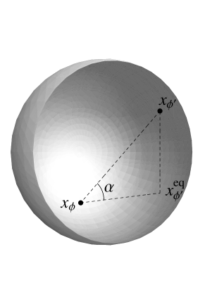
Figure 1: The vertical plane inside the unit ball that contains ${\bf x}_{\phi}$, ${\bf x}_{\phi^{\prime}}$. We denote ${\bf x}_{\phi^{\prime}}^{eq}$ the projection of ${\bf x}_{\phi^{\prime}}$ in the “equatorial” plane $z_{\phi}=\text{cst}$

On the contrary, making ${\mathcal{A}}=M_{2}({\mathbb{C}})$ act on ${\mathcal{H}}={\mathbb{C}}^{2}$, with $D$ a $2$-by-$2$ matrix with distinct non-zero eigenvalues $D_{1},D_{2}$, one obtains [12]

$$d_{D}({\bf x}_{\phi},{\bf x}_{\phi^{\prime}})=\left\{\begin{array}[]{ll}\frac{2}{\lvert D_{1}-D_{2}\rvert}\;d_{Ec}({\bf x}_{\phi},{\bf x}_{\phi^{\prime}})&\text{ if }z_{\phi}=z_{\phi^{\prime}},\\ +\infty&\text{ if }z_{\phi}\neq z_{\phi^{\prime}}.\end{array}\right.$$ (4.15)

Here the eigenvectors of $D$ - chosen as a basis of ${\mathcal{H}}$ - are mapped to the north and south poles of $S^{2}$.

IV.3 Product of the continuum by the discrete

We summarize here the discussion developed in [11, §4.2]. The product of a compact manifold ${\mathcal{M}}$ by the spectral triple (4.1) is the spectral triple $({\mathcal{A}}^{\prime},{\mathcal{H}}^{\prime},D^{\prime})$ where [8]

$${\mathcal{A}}^{\prime}\doteq C^{\infty}({\mathcal{M}})\otimes{\mathbb{C}}^{2},\;{\mathcal{H}}^{\prime}\doteq\Omega^{\bullet}({\mathcal{M}})\otimes{\mathbb{C}}^{2},\;D^{\prime}\doteq(d+d^{\dagger})\otimes{\mathbb{I}}_{2}+\Gamma\otimes D$$ (4.16)

with $\Gamma$ a graduation of $\Omega^{\bullet}({\mathcal{M}})$. An element of ${\mathcal{A}}^{\prime}$ is a pair $a^{\prime}=(f,g)$ of functions in $C^{\infty}({\mathcal{M}})$, and pure states of (the $C^{*}$-closure of) ${\mathcal{A}}^{\prime}$ are pairs

$$x_{i}\doteq(\delta_{x},\delta_{i})$$ (4.17)

where $\delta_{x}\in{\mathcal{P}}(C({\mathcal{M}}))$ is the evaluation at $x\in{\mathcal{M}}$ while $\delta_{i=1,2}$ is one of the two pure states of ${\mathbb{C}}^{2}$ defined in (4.3). Thus ${\mathcal{P}}({\mathcal{A}}^{\prime})$ appears as the disjoint union of two copies of ${\mathcal{M}}$. Explicitly, the evaluation on an element of ${\mathcal{A}}^{\prime}$ reads

$$x_{1}(a^{\prime})=f(x),\quad y_{2}(a^{\prime})=g(y).$$ (4.18)

The spectral distance in this two-sheet model coincides with the geodesic distance $d^{\prime}_{\text{geo}}$ in the manifold ${\mathcal{M}}^{\prime}={\mathcal{M}}\times[0,1]$ with Riemannian metric

$$\left(\begin{array}[]{cc}g_{\mu\nu}&0\\ 0&\frac{1}{\lvert m\rvert}\end{array}\right)$$ (4.19)

where $g_{\mu\nu}$ is the Riemannian metric on ${\mathcal{M}}$. Namely one has [17]

$$d_{D^{\prime}}\left(x_{1},y_{2}\right)=d^{\prime}_{\text{geo}}\left(\left(x,0\right),\left(y,1\right)\right).$$ (4.20)

Non-pure states of ${\mathcal{A}}^{\prime}$ are given by pairs of measures $(\mu,\nu)$ on ${\mathcal{M}}$, normalized to

$$\int_{\mathcal{M}}\,\mathrm{d}\mu+\int_{\mathcal{M}}\,\mathrm{d}\nu=1,$$

whose evaluation on $a^{\prime}=(f,g)$ is

$$\varphi(a)=\int_{\mathcal{M}}f\,\mathrm{d}\mu+\int_{\mathcal{M}}g\,\mathrm{d}\nu.$$ (4.21)

By proposition III.1 one has $d_{D^{\prime}}\leq W_{D^{\prime}}$ where $W_{D^{\prime}}$ is the Monge-Kantorovich distance on ${\mathcal{M}}\cup{\mathcal{M}}$ associated to the cost $d_{D^{\prime}}$. The equality holds for states localized on the same copy:

$$\varphi=(0,\nu),\;\tilde{\varphi}=(0,\tilde{\nu})\quad\text{ or }\quad\varphi=(\mu,0),\;\tilde{\varphi}=(\tilde{\mu},0),$$

since one then has

$$d_{D^{\prime}}(\varphi,\tilde{\varphi})=d_{d+d^{\dagger}}(\varphi,\tilde{\varphi})=W(\varphi,\tilde{\varphi})=W_{D^{\prime}}(\varphi,\tilde{\varphi}).$$ (4.22)

For two states localized on distinct copies, the question is open. It is interesting to notice that one may project back the problem on a single copy of ${\mathcal{M}}$, using the cost function

$$c(x,y)\doteq d_{D^{\prime}}(x_{1},y_{2})\doteq\sqrt{d_{\text{geo}}(x,y)^{2}+\frac{1}{\lvert m\rvert^{2}}}$$

defined on ${\mathcal{M}}$, rather than $d_{D^{\prime}}$ defined on ${\mathcal{M}}\cup{\mathcal{M}}$. The particularity of this single-sheet cost $c$ is that it does not vanish on the diagonal, $c(x,x)=\frac{1}{\lvert m\rvert}\neq 0$.

This might yield interesting perspective in physics: in the description of the standard model of elementary particles in noncommutative geometry [4], the recently discovered Higgs field [5] appears as an extra-component of the metric similar to $\frac{1}{\lvert m\rvert}$, except that it is no longer a constant but a function on ${\mathcal{M}}$. From this perspective the Higgs field represents the cost to stay at the same point of space-time, but jumping from one copy to the other.

V Conclusion

In this contribution we presented preliminary steps towards a definition of a Monge-Kantorovich distance in noncommutative geometry. Given a spectral triple $({\mathcal{A}},{\mathcal{H}},D)$, we introduced a new distance $W_{D}$ on the space of state ${\cal S}({\mathcal{A}})$, which is the exact translation in the noncommutative setting of Kantorovich dual formula, taking as a cost function Connes spectral distance $d_{D}$ on the the pure state space ${\cal P}({\mathcal{A}})$. By construction, $W_{D}=d_{D}$ on ${\cal P}({\mathcal{A}})$, and we showed that the same is true for non-pure states given by convex linear combinations of the same two pure states. Although very restrictive, this condition applies to the interesting example ${\mathcal{A}}=M_{2}({\mathbb{C}})$, showing that $W_{D}=d_{D}$ on a unit ball. At this point two questions remain open and will be the object of future works:

• Is $W_{D}$ equal to $d_{D}$ on the whole of ${\cal S}({\mathcal{A}})$ or only on part of it ?

• Is there a dual formula to $d_{D}$ and/or $W_{D}$ as an infimum (a kind of reverse Kantorovich duality), for instance formula (3.2), or the Wasserstein distance in free probabilities introduced by Biane and Voiculescu [1] ?

These questions are not necessarily linked. If both answers turn out to be positive, this would indicate that computing the spectral distance is exactly a problem of optimal transport, and spectral triples could be used as a factory of cost functions.

References

• [1] P. Biane and D. Voivulescu, A free probability analogue of the Wasserstein metric in the trace state space, GAFA 11 (2001), no. 6, 1125–1138.
• [2] O. Bratteli and D. W. Robinson, Operator algebras and quantum statistical mechanics 1, Springer, 1987.
• [3] Eric Cagnache, Francesco d’Andrea, Pierre Martinetti, and Jean-Christophe Wallet, The spectral distance on Moyal plane, J. Geom. Phys. 61 (2011), 1881–1897.
• [4] A. H. Chamseddine, Alain Connes, and Matilde Marcolli, Gravity and the standard model with neutrino mixing, Adv. Theor. Math. Phys. 11 (2007), 991–1089.
• [5] The Atlas Collaboration, Observation of a new particle in the search for the standard model Higgs boson with the ATLAS detector at the LHC, (2012).
• [6] A. Connes, Compact metric spaces, fredholm modules, and hyperfiniteness, Ergod. Th. & Dynam. Sys. 9 (1989), 207–220.
• [7] Alain Connes, Noncommutative geometry, Academic Press, 1994.
• [8]  , Gravity coupled with matter and the foundations of noncommutative geometry, Commun. Math. Phys. 182 (1996), 155–176.
• [9]  , On the spectral characterization of manifolds, preprint arXiv:0810.2088 (2008).
• [10] Alain Connes and John Lott, The metric aspect of noncommutative geometry, Nato ASI series B Physics 295 (1992), 53–93.
• [11] Francesco D’Andrea and Pierre Martinetti, A view on optimal transport from noncommutative geometry, SIGMA 6 (2010), no. 057, 24 pages.
• [12] Bruno Iochum, Thomas Krajewski, and Pierre Martinetti, Distances in finite spaces from noncommutative geometry, J. Geom. Phy. 31 (2001), 100–125.
• [13] L. V. Kantorovich, On the transfer of masses, Dokl. Akad. Nauk. SSSR 37 (1942), 227–229.
• [14] L. V. Kantorovich and G.S Rubinstein, On a space of totally additive functions, Vestn. Leningrad Univ. 13 (1958), no. 52-58.
• [15] P. Martinetti, Distances en géométrie non-commutative, PhD thesis (2001), arXiv:math–ph/0112038v1.
• [16] Pierre Martinetti, Spectral distance on the circle, J. Func. Anal. 255 (2008), no. 1575-1612.
• [17] Pierre Martinetti and Raimar Wulkenhaar, Discrete Kaluza-Klein from scalar fluctuations in noncommutative geometry, J. Math. Phys. 43 (2002), no. 1, 182–204.
• [18] Marc A. Rieffel, Metric on state spaces, Documenta Math. 4 (1999), 559–600.