Equivalent circuit model of radiative heat transfer

Abstract

Here, we develop a theory of radiative heat transfer based on an equivalent electrical network representation for the hot material slabs in an arbitrary multilayered environment with arbitrary distribution of temperatures and electromagnetic properties among the layers. Our approach is fully equivalent to the known theories operating with the fluctuating current density, while being significantly simpler in analysis and applications. A practical example of the near-infrared heat transfer through the micron gap filled with an indefinite metamaterial is considered using the suggested method. The giant enhancement of the transferred heat compared to the case of the empty gap is shown.

I Introduction

There are two most important heat exchange processes known: thermal conductivity, associated with collective oscillations of atoms (i.e., phonons) or electrons in solids including metals, or with convection in fluids or gases, and radiative heat transfer which is associated to the electromagnetic radiation produced by thermally agitated atoms, e.g., the black body radiation. In this work we concentrate on the latter process which can be dominant when the bodies that exchange heat are separated by gaps (empty or filled with a heterogeneous material that weakly conducts the heat).

As is known, thermal radiation results from fluctuations of charge and current density in matter. This phenomenon is governed by the fluctuation-dissipation theorem FDT (FDT) that relates the mean-square fluctuations of a physical quantity to the dissipation associated with the dynamics of the same quantity. Because in dielectrics the loss is represented by the imaginary part of the permittivity, which may be in turn related to the effective conductivity of the material, the FDT requires the volumetric current density within a dielectric or conducting body to fluctuate. The FDT constitutes the basis of the present day radiative heat transfer theories which deal with the fluctuating currents and treat them as the principal source of thermal radiation. Such a picture places the radiative heat transfer calculations in the framework of classical electromagnetic theory based on the macroscopic Maxwell equations.

Indeed, the well-known theory of radiative heat transfer through narrow vacuum gaps by Polder and van HovePolder belongs to this class. Similar techniques have been recently developed for the cases when radiative heat transfer through micron and even submicron gaps is assisted with nanostructured metamaterials (see, e.g., in Refs. 6, ; new, ; arxivTPV, ). In these approaches the fluctuating current density in the two neighboring media is first obtained from the FDT, following the methodology introduced by Rytov.Rytov3 Next, the electromagnetic field produced by the fluctuating currents is calculated, after which the mean value of the power flow (Poynting vector) across the gap (filled with the metamaterial) is found either with the multiple reflection method,6 ; new or with a more general transfer matrix approach.arxivTPV

Historically, however, thermal agitation of fluctuating currents was first discovered by JohnsonJohnson in electric circuits and the theory of such thermal fluctuations was developed by NyquistNyquist using ideas which were natural for an engineer dealing with networks of lumped elements and transmission lines. Although this theory was a precursor to the FDT, it is still in wide use in the theory of thermal noise at radio and microwave frequencies. The famous Nyquist’s result states that, in any linear passive two-pole (i.e., a single port device with an input represented by two electric contacts) operating at a temperature $T$ the electric thermal fluctuations (in other words, the thermal noise) concentrated within a narrow frequency interval $\Delta\nu$ can be equivalently represented by the fluctuating electromotive force (EMF) $e(t)$, with the mean-square of fluctuations

$$\overline{e^{2}}=4\Theta(\nu,T)R(\nu)\Delta\nu,$$ (1)

where $\Theta(\nu,T)=h\nu/[\exp(h\nu/k_{\rm B}T)-1]$ is Planck’s mean energy of a harmonic oscillator with $h$ and $k_{\rm B}$ being the Planck and Boltzmann constants, respectively, and $R(\nu)$ is the input resistance (real part of the input impedance) of the two-pole. The equivalent EMF is then understood as connected in series with the two-pole, which can be now considered noiseless.

The beauty of this result is in that no knowledge of the internal structure of the electric network is required, and that all the information is contained within just a single parameter: the real part of the frequency-dependent input impedance. In the terminology of FDT, the equivalent EMF in Nyquist’s formula has the role of a generalized force, and the two-pole input impedance is related to the generalized susceptibility of the system. In other words, the Nyquist formula can be obtained by a direct application of FDT to the electric circuit.Rytov3 Note that the fluctuating current appears in this model only as a reaction to a finite number of lumped voltage sources.

In contrast, in the thermal transfer theory based on the full-wave electromagnetic formulation through the fluctuating current density understood as a volume-distributed source, the internal structure of the interacting bodies has to be considered during most of the calculations. Thus, a thermal transfer problem appears in this formulation as a problem with infinite number of degrees of freedom. The final result, however, happens to be expressed in quantities that abstract away the internal structure, such as the reflection coefficients of material half-spaces in the theory of Polder and van Hove.Polder This observation suggests that introducing the distributed fluctuating current can be avoided in many cases. For example, in this work we prove that in stratified media the input impedance concept and the original Nyquist theory can be generalized and used not only in problems related to electric networks, but also in full-wave radiative heat transfer problems. This allows for a significant reduction in complexity of the analysis and makes the theory readily available for practical calculations.

It has to be mentioned that an expression for the equivalent lumped EMF of the thermal noise for the case of a lossy material half-space was first derived by RytovRytov3 using an approach based on the fluctuating current density. This result constitutes the basis of the thermal noise theory of aperture antennas.Pozar ; Kraus Rytov also worked on equivalent four-pole network representation of a hot material slab.Rytov3 Why then these results have not been widely used in the heat transfer problems? Perhaps, it is because the concepts of input impedance and the equivalent circuit description for full-wave electromagnetic problems are largely unknown among theorists working in the field of radiative heat transfer. In applied electromagnetics, however, it is well-known that stratified media can be very efficiently treated within the so-called vector transmission line theoryTret (VTLT) which, in essence, assigns an equivalent transmission line network to every electromagnetic mode (propagating or evanescent) in the system. We would like to stress here that the VTLT is not an approximation: it is a direct consequence of the Maxwell equations when modal expansion is applied to the electromagnetic field in layered structures. The VTLT allows also for a systematic treatment of uniaxial and bi-anisotropic media.

In this work we extend the VTLT in order to include the effect of the fluctuating current density within the layers. In contrast to a few numerical discrete-element models currently available from the literature (e.g., Ref. Syms, ), the theory that we develop here is fully analytical. The generalized theory allows us to prove a complete equivalence between a volumetric multilayered structure and its circuit theory counterpart, which may be visualized as a chain of transmission line segments with equivalent fluctuating voltage sources connected at the ports. When concerned with the radiative heat transfer between the layers, we show that this equivalent network may be reduced to just a series connection of a number of voltage sources representing the fluctuating EMFs and equivalent impedances (each can be under different temperature), thus, recovering in this way the famous Nyquist result, generalized here to the full-wave electromagnetic processes in stratified media. Therefore, the calculation of the radiative heat transfer between the layers reduces in our theory to a number of equivalent circuit theory calculations, which are relatively simple and very similar to what is typically done when considering thermal noise in practical electric networks.Rytov ; Rytov1 ; Rytov2

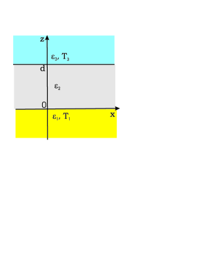
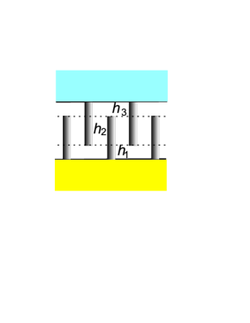
Figure 1: (Color online) (a) – Illustration to the general problem formulation. (b) – A possible implementation of medium 2 suggested in Ref. arxivTPV, transforms the gap into a layered structure filled with so-called hyperbolic metamaterial (see, e.g., in Refs. Smith, ; Narimanov, ; NarimanovLS, ; Biehs, ) formed by carbon nanotubes or metal nanowires. Interdigital arrangement of nanotubes (nanowires) helps keep radiative heat transfer dominating over the thermal conductance through the gap.

II Impedance representation of the classical heat transfer formula

In this section we establish a connection between the classic Polder–van Hove theory of radiative thermal transfer and its representation in terms of the input impedances of the material half-spaces. Formulas by Polder and van Hove for the density of the radiative heat flux (i.e., power flux of the thermal radiation) across the gap between two thick dielectric slabs [the geometry is defined in Fig. 1(a); the slabs are approximated by half-spaces] read as (our notations correspond to Refs. 5, ; 8, ; 1, ):

$$S_{\rm t}=\int\limits_{0}^{\infty}d\omega[\Theta(\omega,T_{1})-\Theta(\omega,T_{3})]M,\quad\Theta(\omega,T_{i})=\frac{\hbar\omega}{e^{\hbar\omega\over k_{\rm B}T_{i}}-1}.$$ (2)

Here $\hbar=h/(2\pi)$, and $T_{i}$ is the absolute temperature of the $i$-th medium ($i=1,3$; $i=2$ represents the gap). If $T_{1}>T_{3}$ the total radiative flux is directed from medium 1 to medium 3 and can we written as $S_{\rm t}=S_{1\rightarrow 3}-S_{3\rightarrow 1}$ where $S_{1\rightarrow 3}$ is the heat flux produced by medium 1 and absorbed in medium 3 and $S_{3\rightarrow 1}$ is the flux produced by medium 3 and absorbed in medium 1. $M$ from (2) is called the radiative heat transfer function.1 It depends on the optical properties of all three media and may be written as the sum $M=M_{p}+M_{e}$, where $M_{p}$ and $M_{e}$ are contributions of propagating and evanescent waves, respectively [note that in this paper we assume the time dependence $\exp(+j\omega t)$ with $j=\sqrt{-1}$]:

$$M_{p}={1\over\pi^{2}}\int\limits_{0}^{k_{0}}N_{p}(\omega,q)q\,dq,\quad N_{p}(\omega,q)={(1-|\Gamma_{12}(q,\omega)|^{2})(1-|\Gamma_{32}(q,\omega)|^{2})\over 4|1-e^{-2j\beta d}\Gamma_{12}(q,\omega)\Gamma_{32}(q,\omega)|^{2}},$$ (3)

$$M_{e}={1\over\pi^{2}}\int\limits_{k_{0}}^{\infty}N_{e}(\omega,q)q\,dq,\quad N_{e}(\omega,q)={{\rm Im}[\Gamma_{12}(q,\omega)]{\rm Im}[\Gamma_{32}(q,\omega)]e^{-2|\beta|d}\over|1-e^{-2|\beta|d}\Gamma_{12}(q,\omega)\Gamma_{32}(q,\omega)|^{2}},$$ (4)

where $\Gamma_{12}$ and $\Gamma_{32}$ are the reflection coefficients of a plane wave harmonic having the spatial frequency (transverse wave number) $q\equiv|{\bf k}_{t}|$ and being incident from a lossless medium 2 (here, medium 2 is free space) to the surfaces of media 1 and 3, respectively, $\beta=\sqrt{k_{0}^{2}-q^{2}}$ is the normal component of the wave vector in medium 2, and $k_{0}=\omega\sqrt{\varepsilon_{0}\mu_{0}}$ is the wave number in medium 2. Function $N(\omega,q)$ is called the spatial spectrum of the radiative heat transfer function. This function was studied in Ref. 5, for the case when photon tunnelling through the vacuum gap was enhanced by surface plasmon-polaritons excited at the gap boundaries. It was shown that the absolute maximum of $N(\omega,q)$ achievable at certain values of $\omega$ and $q$ equals $1/4$ (we discuss this limit with more detail in Section VI).

Let us express reflection coefficients $\Gamma_{12}$ and $\Gamma_{32}$ in (3) and (4) through wave impedances $Z_{1,2,3}$ of the media in regions 1, 2 and 3. The wave impedance defines the ratio between the transverse electric and magnetic fields in a plane wave of a given polarization, i.e., in a given harmonic of the spatial spectrum (see, e.g., in Ref. Tret, ). In terms of the wave impedances,

$$\Gamma_{i2}={Z_{i}-Z_{2}\over Z_{i}+Z_{2}},\quad i=1,\ 3.$$ (5)

For isotropic dielectrics the wave impedances are given by the following expressions (see, e.g., in Ref. Tret, ) for TM-waves and TE-waves, respectively:

$$Z_{i}^{\rm TM}=\eta_{0}{\beta_{i}\over k_{0}\varepsilon_{i}},\quad Z_{i}^{\rm TE}=\eta_{0}{k_{0}\over\beta_{i}},$$ (6)

where $\eta_{0}$ is the characteristic impedance of free space $\eta_{0}=\sqrt{\mu_{0}/\varepsilon_{0}}$, and $\beta_{i}$ denotes the normal component of the wave vector in the $i$-th medium: $\beta_{i}=\sqrt{k_{0}^{2}\varepsilon_{i}-q^{2}}$. If medium 2 is free space (as it is assumed in the classical theory of Ref. Polder, ) $\varepsilon_{i}=1$. For propagating waves $q<k_{0}$ and $Z_{2}$ is real, for evanescent waves $q>k_{0}$ and $Z_{2}$ is imaginary. It is important that the impedance representation (5) of the reflection coefficients is general for all spatial frequencies $q$.

Substituting Eq. (5) into Eq. (3) we obtain after a rather simple algebra:

$$N_{p}={16R_{2}^{2}R_{1}R_{3}\over 4|(Z_{1}+Z_{2})(Z_{2}+Z_{3})+(Z_{1}-Z_{2})(Z_{2}-Z_{3})e^{-2j\beta_{2}d}|^{2}}.$$ (7)

Here and below we denote $R_{i}\equiv{\rm Re}(Z_{i})$ and $X_{i}\equiv{\rm Im}(Z_{i})$. Substituting Eq. (5) into Eq. (4) we easily deduce:

$$N_{e}={4X_{2}^{2}R_{1}R_{3}\,e^{-2|\beta_{2}|d}\over|(Z_{1}+Z_{2})(Z_{2}+Z_{3})+(Z_{1}-Z_{2})(Z_{2}-Z_{3})e^{-2|\beta_{2}|d}|^{2}}.$$ (8)

In this case $\beta_{2}$ has imaginary value and it is taken into account that $Z_{2}=jX_{2}$. Since $X_{2}=0$ for propagating waves and $R_{2}=0$ for evanescent waves, Eqs. (7) and (8) can be unified into an expression suitable for both regions $q<k_{0}$ and $q>k_{0}$:

$$N(\omega,q)={4|Z_{2}|^{2}R_{1}R_{3}|e^{-j\beta_{2}d}|^{2}\over|(Z_{1}+Z_{2})(Z_{2}+Z_{3})+(Z_{1}-Z_{2})(Z_{2}-Z_{3})e^{-2j\beta_{2}d}|^{2}}.$$ (9)

The heat flux density originated from the medium 1 and absorbed in the medium 3 can now be represented as integral over the complete spatial spectrum (both propagating and evanescent):

$$S_{1\rightarrow 3}={1\over\pi^{2}}\int\limits_{0}^{\infty}d\omega\int\limits_{0}^{\infty}qdq\,\Theta(\omega,T_{1})N(\omega,q).$$ (10)

As we show in the next section, Eq. (9) for the spatial spectrum of the heat transfer function $N(\omega,q)$ can be derived from the VTLT in a way that allows for a straightforward generalization of the results of Polder and van HovePolder to the case of stratified uniaxial magneto-dielectric media without a need to introduce the distributed fluctuating currents.

III Radiative heat transfer resulting from an equivalent circuit approach

The possibility to express the radiative heat transfer through the wave impedances of the material layers provides us with an evidence that an equivalent circuit model can be formulated for this problem. Such a model is derived rigorously in Appendix directly from the Maxwell equations, which results in the VTLT generalized to include the effect of thermal fluctuations. Throughout this section, however, we will use simple physical reasoning when possible, in order to keep the derivations easy to grasp.

As in the previous section, we decompose the fluctuating electromagnetic field into plane waves characterized with a certain polarization state, angular frequency $\omega$, and the transverse wave vector ${\bf k}_{t}$. For generality, let us assume that all materials taking part in the heat transfer are optically uniaxial magneto-dielectric media. It is known that in uniaxial magneto-dielectrics the independent polarization states correspond to the TE and TM plane waves. The same holds for a multilayered structure composed of uniaxial magneto-dielectric layers (some of them can be isotropic or even vacuum gaps) under the condition that the anisotropy axes of all layers are aligned. In such a structure the two polarizations are completely independent and can be considered separately. In the following we assume that the anisotropy axis of the layers coincides with the $z$-axis which is perpendicular to the layers.

In Appendix we prove that, in a given layer of the considered multilayered structure ($i$-th layer) being under the temperature $T_{i}$ the transverse components of the time-harmonic fluctuating electric and magnetic fields at the layer interfaces (labeled here with subscripts 1 and 2) are related as follows

$$\left(\begin{array}[]{cc}\overline{\overline{Z}}^{i}_{11}&\overline{\overline{Z}}^{i}_{12}\\ \overline{\overline{Z}}^{i}_{21}&\overline{\overline{Z}}^{i}_{22}\end{array}\right)\cdot\left(\begin{array}[]{c}{\bf n}_{1}\times{{{\bf H}}_{1}^{i}}_{t}\\ {\bf n}_{2}\times{{{\bf H}}_{2}^{i}}_{t}\end{array}\right)-\left(\begin{array}[]{c}{{{\bf E}}_{1}^{i}}_{t}\\ {{{\bf E}}_{2}^{i}}_{t}\end{array}\right)={1\over\sqrt{A_{0}}}\left(\begin{array}[]{c}{\bf e}_{1}^{i}\\ {\bf e}_{2}^{i}\end{array}\right)$$ (11)

where $\overline{\overline{Z}}^{i}_{mn}=\overline{\overline{Z}}^{i}_{mn}(\omega,{\bf k}_{t})$ are the dyadic $Z$-parameters of the chosen layer, and ${\bf e}_{1,2}^{i}$ are the vectorial fluctuating EMFs equivalently representing the thermal-electromagnetic fluctuations within the same layer, and ${\bf n}_{1,2}$ are the external unit normals at the interfaces of the layer. The meaninig of the factor $1/\sqrt{A_{0}}$ is explained further in the text. Eq. (11) generalizes the known result of the VTLT to the case of non-vanishing thermal fluctuations. When the right-hand side of (11) vanishes this equation represents the definition of the impedance matrix of a passive material layer.

The result (11) is obtained in a dyadic form and, thus, is applicable to any polarization state of the electromagnetic field in an anisotropic (not only uniaxial) layer. However, when the states split into the TE and TM waves it is more convenient to work with scalar $Z$-parameters — elements of the $2\times 2$ impedance matrix — which are defined separately for each polarization. For a slab of a uniaxial magneto-dielectric characterized by the permittivity dyadic $\overline{\overline{\varepsilon}}=\varepsilon_{i}^{\perp}\overline{\overline{I}}_{t}+\varepsilon_{i}^{\parallel}{\bf z}_{0}{\bf z}_{0}$ and the permeability dyadic $\overline{\overline{\mu}}=\mu_{i}^{\perp}\overline{\overline{I}}_{t}+\mu_{i}^{\parallel}{\bf z}_{0}{\bf z}_{0}$ (here we understand these parameters as relative to the vacuum permittivity $\varepsilon_{0}$ and the permeability $\mu_{0}$, respectively, with $\overline{\overline{I}}_{t}$ being the unity dyadic in the transverse plane), the $Z$-parameters are (see, e.g., Ref. Tret, ):

$$Z^{i}_{12}=Z^{i}_{21}=j{Z_{i}^{\rm TE,TM}\over\sin(\beta^{\rm TE,TM}_{i}d_{i})},\quad Z^{i}_{11}=Z^{i}_{22}=-j{Z_{i}^{\rm TE,TM}\over\tan(\beta^{\rm TE,TM}_{i}d_{i})},$$ (12)

where $\beta^{\rm TE,TM}_{i}d_{i}$ is the electric thickness of the $i$-th layer, and the wave impedances of a spatial harmonic with wave vector ${\bf k}=(k_{x},k_{y},\beta^{\rm TE,TM}_{i})$ are

$$Z_{i}^{\rm TE}=\eta_{0}{k_{0}\mu_{i}^{\perp}\over\beta^{\rm TE}_{i}},\quad Z_{i}^{\rm TM}=\eta_{0}{\beta^{\rm TM}_{i}\over k_{0}\varepsilon_{i}^{\perp}},$$ (13)

where the propagation constants for the two polarizations are expressed through $q=\sqrt{k_{x}^{2}+k_{y}^{2}}$ as (see, e.g., Tret, ):

$$\beta^{\rm TE}_{i}=\sqrt{{\mu_{i}^{\perp}(k_{0}^{2}\varepsilon_{i}^{\perp}\mu_{i}^{\parallel}-q^{2})\over\mu_{i}^{\parallel}}},\quad\beta^{\rm TM}_{i}=\sqrt{{\varepsilon_{i}^{\perp}(k_{0}^{2}\mu_{i}^{\perp}\varepsilon_{i}^{\parallel}-q^{2})\over\varepsilon_{i}^{\parallel}}}.$$ (14)

Thus, when considering plane waves of fixed polarization and fixed transverse wave number $q\equiv|{\bf k}_{t}|$ such a slab is described by a $2\times 2$ matrix of scalar $Z$-parameters, much like a four-pole network in the circuit theory. Pozar To make the analogy complete, we may introduce the effective “currents” flowing into this four-pole network and relate them to the magnetic fields at the two interfaces of the slab as

$$I_{1,2}^{i,\rm TM}=\sqrt{A_{0}}\,{{\bf k}_{t}\over|{\bf k}_{t}|}\cdot({\bf n}_{1,2}\times{{{\bf H}}_{1,2}^{i}}_{t}),\quad I_{1,2}^{i,\rm TE}=\sqrt{A_{0}}\,{{\bf z}_{0}\times{\bf k}_{t}\over|{\bf k}_{t}|}\cdot({\bf n}_{1,2}\times{{{\bf H}}_{1,2}^{i}}_{t}),$$ (15)

and the effective “voltages” at the input and the output interfaces of the slab

$$V_{1,2}^{i,\rm TM}=\sqrt{A_{0}}\,{{\bf k}_{t}\over|{\bf k}_{t}|}\cdot{{{\bf E}}_{1,2}^{i}}_{t},\quad V_{1,2}^{i,\rm TE}=\sqrt{A_{0}}\,{{\bf z}_{0}\times{\bf k}_{t}\over|{\bf k}_{t}|}\cdot{{{\bf E}}_{1,2}^{i}}_{t}.$$ (16)

The factor $\sqrt{A_{0}}$ where $A_{0}$ is the unit area in the transverse plane ensures that the complex power $V^{i,\rm TE,TM}_{1,2}{I^{i,\rm TE,TM}_{1,2}}^{*}=-A_{0}\,{\bf n}_{1,2}\cdot\left({{\bf E}_{1,2}^{i,\rm TE,TM}}\times{{\bf H}_{1,2}^{i,\rm TE,TM}}^{*}\right)$ is trivially related to the complex Poynting vector of a mode. Then, for a given polarization (TE or TM) relation (11) assumes the form

$$\left(\begin{array}[]{cc}Z^{i}_{11}&Z^{i}_{12}\\ Z^{i}_{21}&Z^{i}_{22}\end{array}\right)\cdot\left(\begin{array}[]{c}I_{1}^{i}\\ I_{2}^{i}\end{array}\right)-\left(\begin{array}[]{c}V_{1}^{i}\\ V_{2}^{i}\end{array}\right)=\left(\begin{array}[]{c}e_{1}^{i}\\ e_{2}^{i}\end{array}\right).$$ (17)

Figure 2: Equivalent four-pole network of a material layer under temperature $T=T_{i}$.

The equivalent circuit that corresponds to this relation is shown in Fig. 2. The two EMFs at the input and the output of this circuit represent the effect of thermal fluctuations inside the chosen layer. The mean square amplitude of these equivalent sources is derived in Appendix using the approach of the distributed fluctuating current. However, one can apply the Nyquist theory directly to the electric circuit in Fig. 2 and obtain the same result. Namely, by disconnecting the load from the output of the four-pole network, i.e., setting $I_{2}^{i}=0$, we eliminate the contribution of $e_{2}^{i}$ and obtain a simple two-pole network with the input impedance $Z_{\rm in}=V_{1}^{i}/I_{1}^{i}=Z_{11}^{i}$. Therefore, the mean square amplitude of the fluctuating EMF $e_{1}^{i}$ within an angular frequency interval $\Delta\omega$ is

$$\overline{(e_{1}^{i})^{2}}=2\Theta(\omega,T_{i}){\rm Re}(Z_{11}^{i}){\Delta\omega\over\pi}$$ (18)

Repeating the same procedure while interchanging the roles of the input and the output one obtains that

$$\overline{(e_{2}^{i})^{2}}=2\Theta(\omega,T_{i}){\rm Re}(Z_{22}^{i}){\Delta\omega\over\pi}$$ (19)

It is evident that, in general, the fluctuating sources $e_{1}^{i}$ and $e_{2}^{i}$ must be partially correlated, because they both represent the fluctuations within the same layer. Therefore, in calculations involving expressions which are quadratic in voltage and (or) current (e.g., power) one may also need the correlation function of these EMFs: $\overline{(e_{1}^{i}e_{2}^{i})}$. As is shown in Appendix, this correlation can be presented as:

$$\overline{(e_{1}^{i}e_{2}^{i})}=2\Theta(\omega,T_{i}){\rm Re}(Z_{12}^{i}){\Delta\omega\over\pi}.$$ (20)

The set of relations (18)–(20) can be also obtained directly from the FDT. Indeed, if one identifies the charges $q_{1,2}^{i}=I_{1,2}^{i}/(j\omega)$ as the state variables of the circuit depicted in Fig. 2 and the EMFs $e_{1,2}$ as the random forces associated with the fluctuations, then the FDT demands that for the fluctuations concentrated within a narrow frequency interval $\Delta\omega$

$$\overline{(e_{n}^{i}e_{m}^{i})}={j\hbar\over 2}\left[(\alpha^{-1})_{mn}^{*}-(\alpha^{-1})_{nm}\right]\coth{\hbar\omega\over 2k_{B}T}\times{\Delta\omega\over\pi},$$ (21)

where $\alpha_{mn}$ are the generalized susceptibilities such that $q_{m}=\sum_{n}\alpha_{mn}(\omega)e_{n}$. It is readily seen that $(\alpha^{-1})_{mn}=j\omega Z_{mn}$. Substituting this into (21) while taking into account the symmetry properties of $Z_{mn}$ we obtain (18)–(20) after dropping the irrelevant contribution resulting from the quantum zero-point fluctuations.

The relations (18)–(20) together with (17) written for both polarizations fully describe the fluctuations within a material layer. A structure formed by many layers can now be equivalently represented by a chain connection of many four-pole networks each representing a layer. Let us now select an arbitrary boundary between a pair of layers in a multilayered structure and find the radiative power flux per unit area of this boundary (Fig. 3).

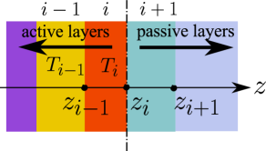
Figure 3: (Color online) An illustration to the calculation of the radiative thermal flux through a selected boundary $z=z_{i}$ in a multilayered structure.

Because the fluctuating EMFs belonging to separate layers are uncorrelated, we may first consider only the sources which are located at $z<z_{i}$, where $z_{i}$ is the position of the selected boundary. We number the layers and the boundaries such that the $i$-th layer is located at $z_{i-1}\leq z\leq z_{i}$. Then, the layers in the half-space $z>z_{i}$ can be considered as passive (no radiation is comming out of them). In the circuit theory terms these layers constitute a load for the other, active, part of the structure located at $z<z_{i}$, and can be equivalently represented by an input impedance, which, for a chain connection of four-pole networks, is given by the following recursive formula

$$Z_{\rm in+}^{i+1}=Z_{11}^{i+1}-{Z_{12}^{i+1}Z_{21}^{i+1}\over Z_{22}^{i+1}+Z_{\rm in+}^{i+2}},$$ (22)

where $Z_{\rm in+}^{i+2}$ is the input impedance of all the layers behind the $(i+1)$-th layer. The recursion is terminated with the input impedance of the last layer which extends up to $z=+\infty$ (it can be, for instance, free space behind the structure), i.e., with the wave impedance of the last layer. Substituting (12) into (22) for the two main polarizations in uniaxial layers we obtain

$$Z_{\rm in+}^{i+1}=Z_{i+1}{Z_{\rm in+}^{i+2}+jZ_{i+1}\tan(\beta_{i+1}d_{i+1})\over Z_{i+1}+jZ_{\rm in+}^{i+2}\tan(\beta_{i+1}d_{i+1})},$$ (23)

where, for brevity, $Z_{i+1}\equiv Z_{i+1}^{\rm TE,TM}$ and $\beta_{i+1}\equiv\beta_{i+1}^{\rm TE,TM}$. Eq. (23) is well-known in the theory of transmission lines.

On the other hand, we may apply Thévenin’s theorem to the active layers located at $z<z_{i}$. Doing this, one first finds the internal impedance of Thévenin’s equivalent circuit:

$$Z_{\rm in-}^{i}=Z_{22}^{i}-{Z_{12}^{i}Z_{21}^{i}\over Z_{11}^{i}+Z_{\rm in-}^{i-1}},$$ (24)

or, after substituting (12),

$$Z_{\rm in-}^{i}=Z_{i}{Z_{\rm in-}^{i-1}+jZ_{i}\tan(\beta_{i}d_{i})\over Z_{i}+jZ_{\rm in-}^{i-1}\tan(\beta_{i}d_{i})},$$ (25)

where $Z_{\rm in-}^{i-1}$ is the internal impedance of the rest of the layers located at $z<z_{i-1}$, and the recursion terminates at the layer which extends down to $z=-\infty$. Note that because here we consider reciprocal structures, the Thévenin impedance $Z_{\rm in-}^{i}$ equals the input impedance of all the layers located at $z<z_{i}$ as seen by a wave incident from the half-space $z>z_{i}$.

Next, the equivalent voltage generator in Thévenin’s theorem (recall that the EMF of this generator is the same as the output voltage of the network under the open circuit condition) can be found recursively as:

$${\cal E}_{\rm g}^{i}=-e_{2}^{i}+{Z_{21}^{i}\over Z_{11}^{i}+Z_{\rm in-}^{i-1}}(e_{1}^{i}+{\cal E}_{\rm g}^{i-1}),$$ (26)

where ${\cal E}_{\rm g}^{i-1}$ is the equivalent EMF of all the sources located at $z<z_{i-1}$. This EMF is defined at the boundary $z=z_{i-1}$. Taking into account relations (18)–(20) and the fact that the EMFs corresponding to distinct layers are not correlated, the mean square amplitude of fluctuations of ${\cal E}_{\rm g}^{i}$ can be expressed after some algebra as

$$\overline{({\cal E}_{\rm g}^{i})^{2}}=\overline{(e_{2}^{i})^{2}}+\left|{Z_{21}^{i}\over Z_{11}^{i}+Z_{\rm in-}^{i-1}}\right|^{2}\overline{(e_{1}^{i})^{2}}-2{\rm Re}\left({Z_{21}^{i}\over Z_{11}^{i}+Z_{\rm in-}^{i-1}}\right)\overline{(e_{1}^{i}e_{2}^{i})}+\left|{Z_{21}^{i}\over Z_{11}^{i}+Z_{\rm in-}^{i-1}}\right|^{2}\overline{({\cal E}_{\rm g}^{i-1})^{2}}\\ =2R^{i}_{\rm th}\Theta(\omega,T_{i}){\Delta\omega\over\pi}+F^{i}\,\overline{({\cal E}_{\rm g}^{i-1})^{2}},$$ (27)

where

$$F^{i}=\left|{Z_{21}^{i}\over Z_{11}^{i}+Z_{\rm in-}^{i-1}}\right|^{2}={|Z_{i}|^{2}\over|Z_{i}\cos(\beta_{i}d_{i})+jZ_{\rm in-}^{i-1}\sin(\beta_{i}d_{i})|^{2}},$$ (28)

and

$$R^{i}_{\rm th}={\rm Re}(Z_{\rm in-}^{i})-F^{i}{\rm Re}(Z_{\rm in-}^{i-1}).$$ (29)

This important result shows that the effect of thermal fluctuations within the $i$-th material layer under the temperature $T_{i}$ is fully equivalent to the effect of fluctuations in a resistance $R^{i}_{\rm th}$ placed under the same temperature.

In other words, Eq. (29) manifests that the input resistance ${\rm Re}(Z_{\rm in-}^{i})$ of a stack of layers can be split into two addends: ${\rm Re}(Z_{\rm in-}^{i})=R^{i}_{\rm th}+F^{i}{\rm Re}(Z_{\rm in-}^{i-1})$. When considered together, these addends represent the total loss in the stack. However, when the thermal fluctuations are of concern, Eq. (29) allows us to separate explicitely a part of the input resistance that appears in the Nyquist formula as being under physical temperature of the $i$-th layer. Thus, the noise produced within the $i$-th layer is associated with $R^{i}_{\rm th}$. The other addend, $F^{i}{\rm Re}(Z_{\rm in-}^{i-1})$, is due to the loss in the layers located below the $i$-th layer, and the thermal noise associated with it is understood as the noise received by the $i$-th layer from the background.

Similar concepts exist, for example, in the antenna theory where the thermal noise of an antenna is represented as a sum of the noise generated locally by the ohmic loss in the antenna (analogous to $R^{i}_{\rm th}$) and the noise received from the environment. The first addend in this case is proportional to the antenna loss resistance (which vanishes for an antenna made of a perfect conductor) and the second term is proportional to the radiation resistance of the antenna.

From Eq. (29), ${\rm Re}(Z_{\rm in-}^{i-1})=R_{\rm th}^{i-1}+F^{i-1}{\rm Re}(Z_{\rm in-}^{i-2})$, therefore, we may as well write

$$R^{i}_{\rm th}={\rm Re}(Z_{\rm in-}^{i})-F^{i}R^{i-1}_{\rm th}-F^{i}F^{i-1}R^{i-2}_{\rm th}-\cdots,$$ (30)

where the series terminates at the layer (with the index $i-M$) that extends to $z=-\infty$, for which $R_{\rm th}^{i-M}={\rm Re}\left(Z_{\rm in-}^{i-M}\right)={\rm Re}\left(Z^{\rm TE,TM}_{i-M}\right)$. We may analogously expand the last addend in (27) which corresponds to the effect of fluctuations in the layers located at $z<z_{i-1}$. Doing so we obtain

$$\overline{({\cal E}_{\rm g}^{i})^{2}}=2R^{i}_{\rm th}\Theta(\omega,T_{i}){\Delta\omega\over\pi}+2F^{i}R^{i-1}_{\rm th}\Theta(\omega,T_{i-1}){\Delta\omega\over\pi}+2F^{i}F^{i-1}R^{i-2}_{\rm th}\Theta(\omega,T_{i-2}){\Delta\omega\over\pi}+\cdots,$$ (31)

Thus, we conclude that the effect of thermal fluctuations in all layers located at $z<z_{i}$ is the same as in a chain of resistors with the values $R_{\rm eff}^{i}=R^{i}_{\rm th}$, $R_{\rm eff}^{i-1}=F^{i}R^{i-1}_{\rm th}$, $R_{\rm eff}^{i-2}=F^{i}F^{i-1}R^{i-2}_{\rm th}$, etc., kept under the temperatures $T_{i}$, $T_{i-1}$, $T_{i-2}$, etc. This result is analogous to the known formula for the thermal noise in cascaded amplifiers, in which case the quantities $F^{i}$ are called the noise factors.

The corresponding equivalent circuit is shown in Fig. 4, in which we split Thévenin’s internal impedance into a reactive part $X_{\rm gen}\equiv{\rm Im}(Z_{\rm in-}^{i})$ and a resistive part ${\rm Re}(Z_{\rm in-}^{i})=\sum\limits_{n}R_{\rm eff}^{i-n}$. Respectively, Thévenin’s EMF splits into a series of uncorrelated fluctuating EMFs: ${\cal E}_{\rm g}^{i}=\sum\limits_{n}{\cal E}_{\rm eff}^{i-n}$, with $\overline{({\cal E}_{\rm eff}^{i-n})^{2}}=(2/\pi)\Theta(\omega,T_{i-n})R_{\rm eff}^{i-n}\Delta\omega$, $n=0,1,2,\ldots,M,$ representing the effect of thermal fluctuations in the layers located at $z<z_{i}$. The rest of the structure at $z>z_{i}$ is modeled by an effective load impedance $Z_{\rm load}\equiv Z_{\rm in+}^{i+1}$.

Figure 4: Thévenin’s equivalent network of thermal noise in layered media.

The radiative heat flux from any layer located at $z<z_{i}$ into the half-space $z>z_{i}$ can now be trivially calculated based on this equivalent circuit. Namely, the power spectral density associated with the plane waves with a given transverse wave vector ${\bf k}_{t}=(k_{x},k_{y})$ and a given angular frequency $\omega$, originated in the slab with the index $i-n$, can be expressed as

$$P^{i-n}_{\omega,{\bf k}_{t}}={1\over\Delta\omega}{{\overline{({\cal E}_{\rm eff}^{i-n})^{2}}}\over|Z_{\rm in-}^{i}+Z_{\rm load}|^{2}}{\rm Re}(Z_{\rm load})={2\over\pi}{\Theta(\omega,T_{i-n})R^{i-n}_{\rm eff}\over|Z_{\rm in-}^{i}+Z_{\rm in+}^{i+1}|^{2}}{\rm Re}\!\left(Z_{\rm in+}^{i+1}\right).$$ (32)

Respectively, for the total radiative heat flux (associated with waves of a selected polarization: TE or TM) into the half-space $z>z_{i}$ we have

$$S_{z>z_{i}}=\sum_{n}\int\limits_{0}^{\infty}d\omega\iint{dk_{x}dk_{y}\over(2\pi)^{2}}\,P^{i-n}_{\omega,{\bf k}_{t}}={1\over 2\pi}\sum_{n}\int\limits_{0}^{\infty}d\omega\int\limits_{0}^{\infty}qdq\,P_{\omega,{\bf k}_{t}}^{i-n}.$$ (33)

The flux crossing the the same boundary in the opposite direction is found by reversing the roles of the active and passive layers.

IV Particular case I: Black body radiation

Let us apply this equivalent circuit theory to calculate the power radiated by a black body per unit of frequency and surface area. We assume that a very thick black body lies in the lower half-space $z<0$ and is under the constant temperature $T$. The upper half-space $z>0$ is empty. We are interested in the thermal radiation into this half-space from the black body surface at $z=0$.

The equivalent circuit for this system is composed of a single resistance $R_{\rm eff}^{(1)}={\rm Re}\!\left(Z_{\rm in-}^{(1)}\right)$, where $Z_{\rm in-}^{(1)}$ is the input impedance of the half-space $z<0$ occupied by the black body, a corresponding fluctuating EMF ${\cal E}_{\rm eff}^{(1)}$, a reactance $X_{\rm gen}={\rm Im}\!\left(Z_{\rm in-}^{(1)}\right)$, and a load $Z_{\rm load}=Z_{\rm in+}^{(2)}=Z^{\rm TE,TM}_{0}$, which is the input impedance of the open half-space at $z>0$.

By definition, the black body absorbs all incoming radiation independently of the frequency or the angle of incidence. Thus, electromagnetically, there are no reflections from such a body which means that it is perfectly impedance-matched to the free space. Therefore, $Z_{\rm in-}^{(1)}=Z^{\rm TE,TM}_{0}$ with

$$Z^{\rm TE}_{0}={\sqrt{\mu_{0}/\varepsilon_{0}}\over\sqrt{1-q^{2}/k_{0}^{2}}},\quad Z^{\rm TM}_{0}=\sqrt{\mu_{0}\over\varepsilon_{0}}\sqrt{1-q^{2}/k_{0}^{2}},$$ (34)

and, using Eq. (32), we may write the power spectral density associated with the radiative heat flux into the open half-space as

$$P_{\omega,{\bf k}_{t}}={2\Theta(\omega,T)\over\pi}{\left[{\rm Re}\left(Z^{\rm TE,TM}_{0}\right)\right]^{2}\over\left|2Z^{\rm TE,TM}_{0}\right|^{2}}=\left\{\begin{array}[]{ll}\Theta(\omega,T)/(2\pi),&q\leq k_{0}\\ 0,&q>k_{0}\end{array}\right.$$ (35)

The result is the same for both polarizations. From here, the total power emitted from the black body by both polarizations per unit of its surface, per unit of frequency is

$${dS\over d\omega}=2\times\iint{dk_{x}dk_{y}\over(2\pi)^{2}}\,P_{\omega,{\bf k}_{t}}={\Theta(\omega,T)\over 4\pi^{3}}\iint\limits_{k_{x}^{2}+k_{y}^{2}<k_{0}^{2}}\,dk_{x}\,dk_{y}={\omega^{2}\over 4\pi^{2}c^{2}}\Theta(\omega,T).$$ (36)

The same result can be, of course, obtained from Planck’s expression for spectral radiance of a black body which reads

$$B_{\omega}(T)={\omega^{2}\over 4\pi^{3}c^{2}}\Theta(\omega,T).$$ (37)

The spectral radiance is defined as the power emitted from the black body surface per unit projected area of the emitting surface, per unit solid angle, per frequency:

$$B_{\omega}(T)={\Delta P_{\rm rad}\over A_{\perp}\Delta\Omega\,\Delta\omega}.$$ (38)

Hence, because in spherical coordinates the projected area $A_{\perp}=A_{0}\cos\theta$, we find

$${dS\over d\omega}=\int_{0}^{2\pi}\int_{0}^{\pi/2}B_{\omega}(T)\cos\theta\sin\theta\,d\theta\,d\varphi={\omega^{2}\over 4\pi^{2}c^{2}}\Theta(\omega,T),$$ (39)

which is the same as the result predicted by the equivalent circuit model.

V Particular case II: generalized Polder-van Hove formula

In this section we derive a generalization of the Polder-van Hove formula applicable to layered uniaxial magneto-dielectrics, using the equivalent circuit model developed in Section III. The geometry of the structure is the same as in Fig. 1 (a). We are interested in the radiative thermal transfer between the media which occupy the half-spaces $z<0$ and $z>d$ (the media with indices 1 and 3). These half-spaces are kept under temperatures $T_{1}$ and $T_{3}$, respectively. The region $0<z<d$ (the region 2) may be filled with another uniaxial medium kept under temperature $T_{2}$, or may be left empty (which is the case of a vacuum gap).

In order to find the radiative heat flux from medium 1 into medium 3 we split the structure at the plane $z=d$, and consider the layers located at $z<d$ as active layers. The half-space $z>d$ plays the role of a load. The equivalent circuit of such a structure can be represented as in Fig. 4, with a pair of resistors $R_{\rm eff}^{(1)}=F^{(2)}R_{\rm th}^{(1)}=F^{(2)}{\rm Re}(Z_{1})$ and $R_{\rm eff}^{(2)}={\rm Re}\!\left(Z_{\rm in-}^{(2)}\right)-R_{\rm eff}^{(1)}$, a pair of the corresponding fluctuating EMFs ${\cal E}_{\rm eff}^{(1)}$ and ${\cal E}_{\rm eff}^{(2)}$, a reactance $X_{\rm gen}={\rm Im}\!\left({Z_{\rm in-}^{(2)}}\right)$, and a complex load $Z_{\rm load}=Z_{3}$.

One may verify that in the vacuum gap case $R_{\rm eff}^{(2)}=0$, which is a consequence of the fact that there is no dissipation in the gap. Evidently, the same conclusion holds when the gap is filled with a lossless medium. Nevertheless, the following derivation is general enough to be applicable to both medium-filled or vacuum gaps, with or without dissipation.

We start with calculating the noise factor $F^{(2)}$. Because $Z_{\rm in-}^{(1)}=Z_{1}$, we obtain from (28):

$$F^{(2)}={|Z_{2}|^{2}\over|Z_{2}\cos(\beta_{2}d)+jZ_{1}\sin(\beta_{2}d)|^{2}}={|1-\Gamma_{12}|^{2}|e^{-j\beta_{2}d}|^{2}\over|1-\Gamma_{12}e^{-2j\beta_{2}d}|^{2}},$$ (40)

where $\Gamma_{12}$ is defined in Section II. Thus, from (32),

$$P^{1\rightarrow 3}_{\omega,{\bf k}_{t}}={2\over\pi}{\Theta(\omega,T_{1})F^{(2)}{\rm Re}(Z_{1})\over|Z_{\rm in-}^{(2)}+Z_{3}|^{2}}{\rm Re}(Z_{3}).$$ (41)

Next, Thévenin’s internal impedance $Z_{\rm in-}^{(2)}$ is found from (25):

$$Z_{\rm in-}^{(2)}=Z_{2}{Z_{1}+jZ_{2}\tan(\beta_{2}d)\over Z_{2}+jZ_{1}\tan(\beta_{2}d)}=Z_{2}{1+\Gamma_{12}e^{-2j\beta_{2}d}\over 1-\Gamma_{12}e^{-2j\beta_{2}d}},$$ (42)

from which the total impedance of the network reads

$$Z_{\rm in-}^{(2)}+Z_{3}={2Z_{2}\over 1-\Gamma_{32}}{1-\Gamma_{12}\Gamma_{32}e^{-2j\beta_{2}d}\over 1-\Gamma_{12}e^{-2j\beta_{2}d}},$$ (43)

where $\Gamma_{32}$ is defined in Section II. Substituting (40) and (43) into (41) we obtain

$$P^{1\rightarrow 3}_{\omega,{\bf k}_{t}}={\Theta(\omega,T_{1})\over 2\pi}{|1-\Gamma_{12}|^{2}|1-\Gamma_{32}|^{2}|e^{-j\beta_{2}d}|^{2}\over|1-\Gamma_{12}\Gamma_{32}e^{-2j\beta_{2}d}|^{2}}{{\rm Re}(Z_{1}){\rm Re}(Z_{3})\over|Z_{2}|^{2}}.$$ (44)

Respectively, the total radiative heat flux associated either with TE or TM polarized waves originated from medium 1 and absorbed in medium 3 is

$$S_{1\rightarrow 3}={1\over\pi^{2}}\int\limits_{0}^{\infty}d\omega\int\limits_{0}^{\infty}qdq\,\Theta(\omega,T_{1})N(\omega,q),$$ (45)

where

$$N(\omega,q)={|1-\Gamma_{12}|^{2}|1-\Gamma_{32}|^{2}|e^{-j\beta_{2}d}|^{2}\over|1-\Gamma_{12}\Gamma_{32}e^{-2j\beta_{2}d}|^{2}}{{\rm Re}(Z_{1}){\rm Re}(Z_{3})\over 4|Z_{2}|^{2}}.$$ (46)

In the vacuum gap case, the wave impedance $Z_{2}$ and the propagation factor $\beta_{2}$ are purely real (imaginary) for the propagating waves (evanescent waves) in the gap. Therefore, because $Z_{i}=Z_{2}(1+\Gamma_{i2})/(1-\Gamma_{i2})$, $i=1,3$, we have

$${\rm Re}(Z_{i})=\left\{\begin{array}[]{rl}|Z_{2}|{\displaystyle 1-|\Gamma_{i2}|^{2}\over\displaystyle|1-\Gamma_{i2}|^{2}},&\mbox{(propagating waves),}\\[10.00002pt] -|Z_{2}|{\displaystyle 2\,{\rm Im}(\Gamma_{i2})\over\displaystyle|1-\Gamma_{i2}|^{2}},&\mbox{(evanescent waves),}\end{array}\right.$$ (47)

which results in the Polder-van Hove formulas when substituted into (45) and (46). However, the more general result represented by Eqs. (45)–(46) holds for arbitrary uniaxial magneto-dielectric media filling the gap. It is easy to verify that Eq. (46) can be as well written in form (9).

Moreover, in general, when the gap is filled with a lossy medium and $T_{2}\neq 0$ one also has to take into account the radiative heat flux to medium 3 that is originated in the gap (i.e., in medium 2). The power spectral density associated with it is, from Eq. (32),

$$P^{2\rightarrow 3}_{\omega,{\bf k}_{t}}={2\over\pi}{\Theta(\omega,T_{2})R_{\rm eff}^{(2)}\over|Z_{\rm in-}^{(2)}+Z_{3}|^{2}}{\rm Re}(Z_{3})={\Theta(\omega,T_{2})\over 2\pi}{|1-\tilde{\Gamma}_{12}|^{2}|1-\Gamma_{32}|^{2}|\over|1-\tilde{\Gamma}_{12}\Gamma_{32}|^{2}}{R_{\rm eff}^{(2)}{\rm Re}(Z_{3})\over|Z_{2}|^{2}},$$ (48)

where $\tilde{\Gamma}_{12}=\Gamma_{12}e^{-2j\beta_{2}d}$ is the reflection coefficient defined at the plane $z=d$. One may note that (48) has the same form as (44) with $d=0$ and one of the wave impedances replaced by the effective resistance $R_{\rm eff}^{(2)}$. This is the consequence of the fact that when the thickness of the middle layer increases, $\tilde{\Gamma}_{12}\rightarrow 0$, $R_{\rm eff}^{(2)}\rightarrow{\rm Re}(Z_{2})$, and (48) reduces to the Polder-van Hove’s result for two media in direct contact.

VI Antenna theory and circuit theory concepts applied to radiative heat transfer

In this section, in order to better understand the circuit model developed in this work, we establish a connection between our model and the classical theory of noise in receiving antennas. We consider the radiative heat transfer example from Section V and employ an analogy between the heat-receiving half-space (medium 3) and a loaded receiving antenna. More exactly, in this analogy the unit area of the interface between the media 2 and 3 is treated as an aperture antenna that receives the power of thermal radiation from the half-space $z<d$ and delivers it to medium 3 which is understood as the antenna load. In what follows, we assume that medium 2 is lossless, therefore, all the radiative heat delivered to medium 3 is generated in medium 1.

The equivalent circuit of this problem is the same as the one discussed in Section V with $R_{\rm eff}^{(2)}=0$. Thus, in the antenna analogy there is one noise source with the internal impedance $Z_{\rm in-}^{(2)}\equiv Z_{\rm A}\equiv R_{\rm A}+jX_{\rm A}$, where $X_{\rm A}=X_{\rm gen}$ is the antenna reactance and $R_{\rm A}=F^{(2)}{\rm Re}(Z_{1})$ is the radiation resistance of the antenna. Such analogy signifies that the effective radiation resistance of an aperture equals the real part of the input impedance of the half-space seen from the aperture. The antenna load is represented in this analogy by the impedance $Z_{\rm load}=Z_{3}$ which is the wave impedance of medium 3.

As is known from the theory of noise in lossless antennasPozar (an aperture by itself has no loss), the mean-square EMF $\overline{e^{2}}$ of the thermal noise of a directive antenna (e.g., a radio telescope) is given by the Nyquist formula (1), in which one inserts the radiation resistance of the antenna [as $R(\nu)$] and the effective temperature of the area of the sky to which the antenna is directed (which is medium 1 under temperature $T=T_{1}$ in our analogy). Applying this to the antenna equivalent circuit, we may write for the noise power at the antenna load:

$$P_{\rm out}={\overline{e^{2}}\over|Z_{\rm A}+Z_{3}|^{2}}{\rm Re}(Z_{3})={2\over\pi}{\Theta(\omega,T_{1})R_{\rm A}\over|Z_{\rm A}+Z_{3}|^{2}}{\rm Re}(Z_{3}).$$ (49)

For our example of a lossless medium 2, $R_{\rm A}={\rm Re}\left(Z_{\rm in-}^{(2)}\right)$, which brings us to the same result as the more general cascade-circuit model (41), i.e., $P_{\rm out}=P^{1\rightarrow 3}_{\omega,{\bf k}_{t}}$. Let us also note that if there would be no separating layer, then $Z_{\rm A}$ would be simply equal to the wave impedance of medium 1. With the separation layer in place, antenna model calculation is equivalent to calculation of input impedance of a transmission-line section loaded with a known impedance [Eq. (42)].

It is worth noting that the tight connection between the model of the present paper and the theories of noise in antennas and cascaded electric networks allows one to better understand optimal conditions for radiative heat transfer through composite layers and, consequently, to design these material structures aiming for desired and optimized performance. In particular, from (49) and (41) we see that the problem of maximizing radiative heat transfer for given layer temperatures reduces to an equivalent problem of matching a generator to a load. Let us discuss this issue assuming for simplicity, that the media 1 and 3 are the same, i.e., $Z_{1}=Z_{3}$. At the first glance, it appears that the optimal heat transfer is ensured if we simply connect the two equivalent media together (or fill the gap with the same medium as those 1 and 3). However, this is true only if the wave impedance is real. For complex $Z_{1}$ and $Z_{3}$ (which is realistic even for propagating modes in view of losses in the media), the best radiative heat transfer corresponds to the conjugate impedance matching $Z_{1}=Z_{3}^{*}$ when the negative reactance of one of two media is compensated by the positive reactance of the other one. Then, the spatial spectrum of the heat transfer function in accordance to (9) turns to $N=1/4$ whereas for the direct contact of two equivalent media with wave impedance $Z=R+jX$ we have $N=R^{2}/|2Z|^{2}$. This tells us that the radiative heat transfer through a properly filled gap can be in principle made larger than that through the direct contact of two equivalent media.

In Ref. arxivTPV, it was proposed to insert a slab of the so-called indefinite medium between media 1 and 3 [Fig. 1 (b)]. Indefinite media (also called hyperbolic metamaterialsSmith ) are uniaxial dielectrics characterized by the permittivity tensor that has opposite signs of the longitudinal and transverse components. Such filling allows for enhancement of the heat transfer by increasing the noise factor $F^{(2)}$. This factor increases compared to the vacuum gap because indefinite media support propagation of spatial harmonics with high transverse wavenumbers, which would otherwise be evanescent in the gap [notice the exponential factor in Eq. (40)]. For such waves, $F^{(2)}$ dramatically increases at the spatial frequencies that correspond to the minima of the denominator of Eq. (40). However, it is not straightforward to ensure proper impedance match in such structures. In this view, the structure suggested and studied in Ref. arxivTPV, is not fully optimal, although it still demonstrates that a specifically crafted filling may dramatically enhance the radiative heat transfer through the gap.

The transmission line analogy, however, suggest an immediate possibility to circumvent the problem of impedance conjugate match. The key is to make the wave impedances of all three media real (at least, approximately) and equal in all layers. This can be realized using a wire medium in region 2 which extends inside regions 1 and 3. Indeed, it is known that wire media support propagating TEM modes with high spatial frequencies (transverse wave numbers) $q$, including $q>k_{0}$ and limited only by the period of the wire array (see, e.g., in Ref. AM, ). Wires should be good conductors at the frequency of interest, and the background media nonconducting. If the wires extend over all three regions and none of them has a conducting background, then these TEM modes will exist and have real wave impedance everywhere in the system, in principle allowing the conjugate match of the load to the heat source for a wide range of spatial frequencies $q$.

In the present paper we, however, do not present the studies of the heat transfer optimization keeping these results for our next publications. Instead, in the next section we report some numerical results illustrating the applicability of our model for solving practical problems.

VII Numerical example: Radiative thermal transfer through a nanostructured layer

In order to demonstrate the applicability of the developed theory to real-world problems, we calculate in this section the spectral density of the radiative heat flux absorbed in medium 3 of the structure depicted in Fig. 1 (b):

$$s_{13}\equiv{dS_{1\rightarrow 3}\over d\omega}={1\over 2\pi}\int\limits_{0}^{\infty}P^{1\rightarrow 3}_{\omega,{\bf k}_{t}}\,qdq.$$ (50)

We compare the heat transferred across the vacuum gap with that transferred across the gap filled with either normally oriented metal-state single-wall carbon nanotubes (CNT) or with similarly oriented golden (Au) nanowires. Calculation for the array of CNT is done in order to validate the present model using the exact simulations of Ref. arxivTPV, . Calculations for metal nanowires are done in order to confirm or decline the effect of giant enhancement of radiative heat transfer in the near infrared (IR) range due to the presence of nanowires. This effect was predicted but not studied in Ref. arxivTPV, . In accordance with the theory presented above, all calculations are done for homogenized media. The homogenization models for $i$-th medium results in explicit formulas for $\varepsilon_{i}^{\perp}$ and $\varepsilon_{i}^{\parallel}$ (whereas $\mu_{i}^{\perp}=\mu_{i}^{\parallel}=1$).

The mid-IR homogenization model for the array of CNT was described and validated in Ref. Nefedov, . The parameters of the array of CNT correspond to those of Ref. arxivTPV, [see also in Fig. 1 (b)]. The homogenization model for aligned metal nanowires representing their array as a layer of an indefinite material was described in Ref. Elser, . It is applicable to the visible and near-IR ranges where it offers a rather high accuracy for optically dense arrays of rather thin wires. Practically, for the band $\lambda=$1–2$\ \mu$m one needs the period below 300–600 nm and the wire diameter of the order of the skin depth in the metal or smaller.AM For Au in this wavelength range it means that the thickness of the wires should not exceed 20–50 nm.

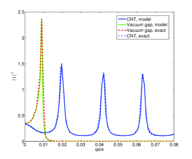
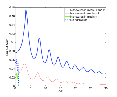
Figure 5: (Color online) (a) – Coefficient $|\tau|^{2}=4|Z_{1}/R_{1}|^{2}N$ at $\lambda=7.5\ \mu$m versus normalized spatial frequency $qa/\pi$ for the gap filled with free space and for that filled with an array of CNT. Dashed lines – exact (beyond homogenization) simulations from Ref. arxivTPV, . Solid lines – analytical calculations in accordance to the present model. (b) – Spatial spectrum $N$ of the radiative heat transfer function versus dimensionless spatial frequency $q/k$ at $\lambda=1.5\ \mu$m. Calculations are done for four cases – nanowires are only in medium 2, nanowires are in both media 1 and 2, nanowires are in medium 1 only and nanowires are absent.

In both cases (CNT in the mid-IR range and nanowires in the near IR) the presence of the metamaterial enhances the radiative heat transfer. This effect results from the conversion of TM-polarized evanescent waves into propagating ones in the effective indefinite material filling the gap.arxivTPV ; NarimanovLS ; Biehs Respectively, in this section we analyze only that part of the radiative heat which is transferred by TM-polarized waves.

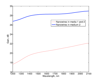
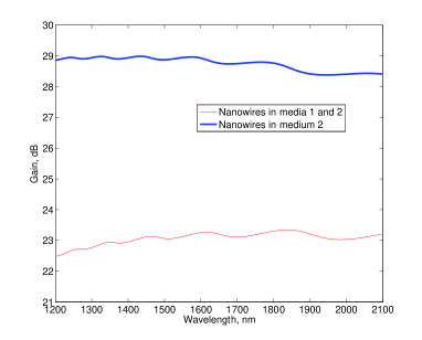
Figure 6: (Color online) The gain in the spectral density of the transferred radiative heat flux due to the presence of nanowires (two cases of their arrangement). (a) – Gap of thickness $d=2\ \mu$m. (b) – Gap of thickness $d=0.5\ \mu$m.

In this numerical example we neglect the contribution of thermal sources located in medium 2 (i.e., in CNT and nanowires). The impact of thermal production and absorption in medium 2 will be evaluated in our next paper, where we will also consider thermo-photovoltaic applications of our present model. As is clear from Fig. 1 (b), medium 2 in the gap is a triple-layered structure, therefore, there are in total five material layers in the whole structure. However, since in this example we neglect the thermal processes in the gap, we may replace the layers in the gap by a single equivalent four-pole network. Its $Z$-matrix, $Z_{mn}^{(2)}$, is obtained in a standard manner from its transfer matrix,Tret with the latter being a product of transfer matrices of effectively homogeneous anisotropic layers with thicknesses $h_{1}$, $h_{2}$ and $h_{3}$. Next, the power spectral density $P^{1\rightarrow 3}_{\omega,{\bf k}_{t}}$ in Eq. (50) is calculated from Eq. (41) where the noise factor is $F^{(2)}=\left|Z_{21}^{(2)}\right|^{2}/\left|Z_{11}^{(2)}+Z_{1}\right|^{2}$ [Eq. (28)], and the internal impedance is $Z_{\rm in-}^{(2)}=Z_{22}^{(2)}-Z_{12}^{(2)}Z_{21}^{(2)}/\left(Z_{11}^{(2)}+Z_{1}\right)$ [Eq. (24)].

In Fig. 5 (a) we depict the energy transfer coefficient $|\tau|^{2}$ introduced in Ref. arxivTPV, [Eq. (12) of Ref. arxivTPV, ] which differs from our heat transfer spatial spectrum $N(\omega,q)$ defined by Eq. (10), by the factor $4|Z_{3}|^{2}/R_{1}R_{3}$. In the present case media 1 and 3 are equivalent (heavily doped silicon), i.e., $Z_{1}=Z_{3},\ R_{1}=R_{3}$. All parameters in the calculation illustrated by Fig. 5 (a) correspond to those from Ref. arxivTPV, . The value $|\tau|^{2}$ is calculated at wavelength $\lambda=7.5\ \mu$m as a function of the normalized spatial frequency $qa/\pi$, where $a=20$ nm is the period of the CNT array in the domains $h_{1}=d/3$ and $h_{3}=d/3$, where the gap thickness is $d=1\ \mu$m. In the domain $h_{2}=d/3$ the array period is equal $a_{2}=\sqrt{20}$ nm. Heavily doped silicon supports so-called surface plasmon-polariton (SPP) waves generated on the surfaces of the Si half-spaces at $(qa/\pi)=0.01$ in the case when the gap is empty. The value $q=0.01\pi/a$ nearly corresponds to $q=1.8k_{0}$, where $k_{0}$ is the free-space wave number. The manifestation of this SPP is the maximum of the corresponding curve in Fig. 5 (a). Dashed curves in Fig. 5 (a) correspond to exact simulations of Ref. arxivTPV, which take into account the microstructure of the material layer in the gap. In Fig. 5 (a) we show only the region of spatial frequencies $(qa/\pi)\leq 0.08$ in which the difference between the exact and homogenized models of the CNT array is negligibly small (see Ref. arxivTPV, ). For both empty gap and gap filled with CNT the agreement between our model and the exact simulations is excellent. Local maxima of the transmittance spatial spectrum for the gap filled with CNT correspond to the thickness resonances of spatial harmonics [in presence of CNT the whole region $(qa/\pi)\leq 0.08$ corresponds to propagating plane waves, though the inequality $q>k_{0}$ holds for $(qa/\pi)>5.6\cdot 10^{-3}$]. Fine agreement between our circuit model and exact simulations pertains at other wavelengths besides the ones mentioned in Figs. 5 (a,b), because with our circuit model we also have reproduced the frequency dependence of the gain in the heat transfer $G(\omega)=s_{13}^{(CNT)}(\omega)/s_{13}^{(0)}(\omega)$, calculated in Ref. arxivTPV, . Here $s_{13}^{(0)}$ corresponds to the vacuum gap and $s_{13}^{(CNT)}$ corresponds to the gap filled with CNT.

In Fig. 5 (b) we present the dependence $N(q,\lambda^{*})$ for the case when the gap $d=2\ \mu$m is filled with golden nanowires. The complex permittivity of gold in the range $\lambda=1\dots 2\ \mu$m was taken from Ref. JC, . Regions 1 and 3 in this case are filled with doped germanium used in real thermo-photovoltaic systems whose complex permittivity was taken from Ref. Ge, . Function $N(q,\lambda^{*})$ was calculated for nanowires with volume fraction $p=0.2$ in the domains $h_{1}$ and $h_{3}$ and $p=0.4$ in the domain $h_{2}$ (when $h_{1}=h_{2}=h_{3}$). Here $\lambda^{*}=1.5\ \mu$m has been chosen having in mind possible thermophotovoltaic applications (at this wavelength the doped Ge has nearly maximal photovoltaic spectral response). The result for $N$ (thick solid curve) was compared with that for the empty gap $d=2\ \mu$m (thin dashed curve) at the same wavelength.

It has to be mentioned that the structure shown in Fig. 1 (b) with free-standing metal nanowires is an abstraction — in a feasible structure nanowires are partially submerged into the host material. Therefore we have also calculated the function $N(q,\lambda^{*})$ for the case when Au nanowires are semi-infinite and have the same volume fraction $p=0.3$ in media 1 and 2. This calculation [thick dashed curve in Fig. 5 (b)] is done in order to understand how the extension of nanowires into medium 1 changes the radiative heat transfer. In this case the gap is uniformly filled, i.e., in the the structure shown in Fig. 1 (b), $h_{2}=h_{3}=0$ and $h_{1}=d$. In this case the nanowres touch the surface of medium 3 and the thermal transfer by the direct thermal conductance may be of significance, in addition to the radiative one. This effect is not considered in the present paper. Additionally, we have studied the case when nanowires with $p=0.3$ are located only in medium 1 and the gap is empty [thin solid curve in Fig. 5 (b)].

We can see in Fig. 5 (b) that the integral increase of $N(q)$ with respect to the empty gap is very significant for both cases when the nanowires fill in the gap. Function $N(q)$ in the case of the vacuum gap has two local maxima in the region $q<k_{0}$ resulting from Fabry-Perot resonances. Because the structure is not fully impedance-matched these maxima are much smaller than the achievable limit $N=1/4$ and $N(q)$ vanishes fast at $q>k_{0}$. Unlike the situation illustrated by Fig. 5 (a) the real part of the complex permittivity of Ge at $\lambda=1.5\ \mu$m is positive and SPP cannot be excited. Since the value of $N(q)$ for the empty gap is so small, the gain granted by Au nanowires to the heat transfer between two half-spaces of Ge turns out to be larger than that offered by CNT to the heat transfer between two half-spaces of Si calculated in Ref. arxivTPV, .

The presence of nanowires only in medium 1 turns out to be destructive for the amplitude of $N$. In this case medium 1 is an indefinite metamaterial, and the mismatch between medium 1 and free space increases. However, if nanowires are present in both media 1 and 2, noticeable values of $N$ keep for $q>k_{0}$. The case when nanowires are located only in medium 2 is the best one: it corresponds to the smallest mismatch between the media.

The dependencies shown in Fig. 5 (b) are typical for every $\lambda$ in the band of the photovoltaic operation of Ge ($\lambda=1-2\ \mu$m). As a result, due to the presence of nanowires the heat transfer gain $G=s_{13}^{(NW)}/s_{13}^{(0)}$ is almost uniform over a wide range of wavelengths. Here $s_{13}^{(NW)}$ corresponds to the case of nanowires in the gap and $s_{13}^{(0)}$ corresponds to the vacuum gap. In Fig. 6 (a) we present the gain in dB, i.e., $10\log_{10}G$ calculated for the case $d=2\ \mu$m. The huge gain keeps for the interval of values $d=0.5\dots 5\ \mu$m. In Fig. 6 (b) we show the same gains for the case $d=0.5\ \mu$m. We can conclude that the presence of Au nanowires in the micrometer or submicron gap can increase the near-IR energy transfer across the gap by 3 orders of magnitude. This result confirms the expectations of Ref. arxivTPV, .

VIII Conclusions

In this work we have formulated an equivalent circuit theory of the radiative heat transfer in uniaxial stratified magneto-dielectric media. We have proven that the effect of thermal-electromagnetic fluctuations in such structures can be fully determined without an explicit knowledge of the microstructure of the layers, as well as without a need to employ any calculations based on distributed fluctuating currents. Instead, the only physical characteristic on which we base our theory is the effective input impedance of a stack of layers, which can be obtained for any spatial harmonic of the field (including both propagating and evanescent waves) using the methods of VTLT. We have shown that such impedance representation, while being in full agreement with sophisticated full-wave methods known from the literature, results in simple formulas analogous to Nyquist theory-based formulas for thermal noise in cascaded electric circuits (for example, cascaded amplifiers). Therefore, with this model some important concepts from the theory of electric networks (conjugate-impedance match, optimal filtering, etc.) can be imported into the field of radiative thermal transfer in multilayered structures.

From the point of view of practical implementations, the developed equivalent circuit approach offers significant simplifications as compared to the known theories of radiative heat transfer based on distributed fluctuating currents. Without any modifications, our method can be used in heat transfer studies in uniaxial anisotropic media that include micron and (or) submicron-thick layers. Moreover, our model is applicable to radiative heat transfer in composite or nanostructured layers (if these layers are effectively homogeneous for spatial harmonics of the electromagnetic field which transfer the radiative heat), and is readily generalizable to stratified bi-anisotropic and spatially dispersive materials. Therefore, we hope that our work may significantly enlarge the scope of the radiative heat transfer research in composites, especially in nanostructured metamaterials. We believe that this may lead to new opportunities in the design of efficient thermal energy harvesting devices, like thermophotovoltaic converters and such.

Appendix: Nyquist formula for a reciprocal anisotropic and lossy magneto-dielectric slab

We consider a uniaxial magneto-dielectric slab described by the macroscopic Maxwell equations for the time-harmonic fields

$$\nabla\times{\bf E}=-j\omega\overline{\overline{\mu}}_{\rm a}\cdot{\bf H}-{\bf J}^{m},\quad\nabla\times{\bf H}=j\omega\overline{\overline{\varepsilon}}_{\rm a}\cdot{\bf E}+{\bf J}^{e},$$ (51)

with the absolute permittivity and permeability dyadics of the form $\overline{\overline{\varepsilon}}_{\rm a}=\varepsilon_{0}(\varepsilon^{\perp}\overline{\overline{I}}_{t}+\varepsilon^{\parallel}{\bf z}_{0}{\bf z}_{0})$ and $\overline{\overline{\mu}}_{\rm a}=\mu_{0}(\mu^{\perp}\overline{\overline{I}}_{t}+\mu^{\parallel}{\bf z}_{0}{\bf z}_{0})$. We assume that the material of the slab is lossy, therefore, by the fluctuation-dissipation theorem (at non-zero temperature) there appear fluctuating external currents ${\bf J}^{e}$ and ${\bf J}^{m}$ in the slab. The explicit form of these currents is not important at this stage. As in the main text, here we use the convention in which the time-harmonic quantities are understood as root mean square (rms) values.

Let the fields ${\bf E}^{\prime}$, ${\bf H}^{\prime}$ be an arbitrary solution of the Maxwell equations (51) with ${\bf J}^{e}={\bf J}^{m}=0$ within the slab. Then, considering the two systems of Maxwell equations with non-zero sources and with vanishing sources, respectively, we can form the Lorentz lemma

$$\nabla\cdot({\bf E}\times{\bf H}^{\prime}-{\bf E}^{\prime}\times{\bf H})={\bf E}^{\prime}\cdot{\bf J}^{e}-{\bf H}^{\prime}\cdot{\bf J}^{m}.$$ (52)

Integrating it over the volume $V$ of the slab, we obtain the reciprocity relation

$$\int_{S_{1}}{\bf n}_{1}\cdot({\bf E}\times{\bf H}^{\prime}-{\bf E}^{\prime}\times{\bf H})\big{|}_{S_{1}}\,dS+\int_{S_{2}}{\bf n}_{2}\cdot({\bf E}\times{\bf H}^{\prime}-{\bf E}^{\prime}\times{\bf H})\big{|}_{S_{2}}\,dS=\int_{V}({\bf E}^{\prime}\cdot{\bf J}^{e}-{\bf H}^{\prime}\cdot{\bf J}^{m})\,dV,$$ (53)

where $S_{1,2}$ are at the two interfaces of the slab, and ${\bf n}_{1,2}$ are the outer unit normals to these surfaces, respectively.

One may select any solution of the uniform Maxwell equations within the slab for the fields ${\bf E}^{\prime}$, ${\bf H}^{\prime}$. For us it is convenient to use the one that has the form

$${\bf E}^{\prime}({\bf r})={\bf E}^{\prime}_{-{\bf k}_{t}}(z)e^{j{\bf k}_{t}\cdot{\bf r}},\quad{\bf H}^{\prime}({\bf r})={\bf H}^{\prime}_{-{\bf k}_{t}}(z)e^{j{\bf k}_{t}\cdot{\bf r}},$$ (54)

where the $z$-axis is orthogonal to the slab and the real vector ${\bf k}_{t}$ lies in the plane of the slab (the $xy$ plane). Physically, such a form corresponds to a superposition of plane waves with the same transverse wavenumber: $-{\bf k}_{t}$. In Eq. (54), ${\bf E}^{\prime}_{-{\bf k}_{t}}$ and ${\bf H}^{\prime}_{-{\bf k}_{t}}$ define the field solution profile within the slab as a function of $z$.

Substituting (54) into the reciprocity relation (53), we obtain (the first slab interface is at $z=z_{1}$ and the second one is at $z=z_{2}$)

$${\bf n}_{1}\cdot({\bf E}_{{\bf k}_{t}}\times{\bf H}^{\prime}_{-{\bf k}_{t}}-{\bf E}^{\prime}_{-{\bf k}_{t}}\times{\bf H}_{{\bf k}_{t}})\big{|}_{z=z_{1}}+{\bf n}_{2}\cdot({\bf E}_{{\bf k}_{t}}\times{\bf H}^{\prime}_{-{\bf k}_{t}}-{\bf E}^{\prime}_{-{\bf k}_{t}}\times{\bf H}_{{\bf k}_{t}})\big{|}_{z=z_{2}}=\\ \int_{z_{1}}^{z_{2}}({\bf E}^{\prime}_{-{\bf k}_{t}}\cdot{\bf J}^{e}_{{\bf k}_{t}}-{\bf H}^{\prime}_{-{\bf k}_{t}}\cdot{\bf J}^{m}_{{\bf k}_{t}})\,dz,$$ (55)

where we have decomposed the fluctuating currents ${\bf J}^{e,m}$ and the fields ${\bf E}$, ${\bf H}$ into plane waves using the Fourier transform defined as

$${\bf F}({\bf r})={A_{0}\over(2\pi)^{2}}\iint{\bf F}_{{\bf k}_{t}}(z)e^{-j{\bf k}_{t}\cdot{\bf r}}\,d^{2}{\bf k}_{t},\quad{\bf F}_{{\bf k}_{t}}(z)={1\over A_{0}}\iint{\bf F}({\bf r})e^{j{\bf k}_{t}\cdot{\bf r}}\,d^{2}{\bf r},$$ (56)

where $A_{0}$ is the unit area in the $xy$-plane, and ${\bf F}$ can be any of the fields or currents.

Eq. (55) is the reciprocity relation for the wave components characterized with a fixed transverse wavenumber. In order to simplify further writing we will use the notation ${\bf F}_{1,2}\equiv{\bf F}_{\pm{\bf k}_{t}}(z_{1,2})$ with ${\bf F}$ being any of the fields or currents. Then, noticing that only transverse components of the fields play any role on the left-hand side of (55) we rewrite it as

$${\bf n}_{1}\cdot({{\bf E}_{1}}_{t}\times{{\bf H}^{\prime}_{1}}_{t}-{{\bf E}^{\prime}_{1}}_{t}\times{{\bf H}_{1}}_{t})+{\bf n}_{2}\cdot({{\bf E}_{2}}_{t}\times{{\bf H}^{\prime}_{2}}_{t}-{{\bf E}^{\prime}_{2}}_{t}\times{{\bf H}_{2}}_{t})=\\ {{\bf E}^{\prime}_{1}}_{t}\cdot({\bf n}_{1}\times{{\bf H}_{1}}_{t})-{{\bf E}_{1}}_{t}\cdot({\bf n}_{1}\times{{\bf H}^{\prime}_{1}}_{t})+{{\bf E}^{\prime}_{2}}_{t}\cdot({\bf n}_{2}\times{{\bf H}_{2}}_{t})-{{\bf E}_{2}}_{t}\cdot({\bf n}_{2}\times{{\bf H}^{\prime}_{2}}_{t}).$$ (57)

Let us remind that the quantities ${{\bf E}^{\prime}_{1,2}}_{t}$ and ${{\bf H}^{\prime}_{1,2}}_{t}$ have the meaning of the transverse components of the electric and magnetic fields at the interfaces of a source-free magneto-dielectric slab. Therefore, as follows from the vector transmission line theory (VTLT) for such slabs, these components are related by the impedance matrix of the slab

$$\left(\begin{array}[]{c}{{\bf E}^{\prime}_{1}}_{t}\\ {{\bf E}^{\prime}_{2}}_{t}\end{array}\right)=\left(\begin{array}[]{cc}\overline{\overline{Z}}_{11}&\overline{\overline{Z}}_{12}\\ \overline{\overline{Z}}_{21}&\overline{\overline{Z}}_{22}\end{array}\right)\cdot\left(\begin{array}[]{c}{\bf n}_{1}\times{{\bf H}^{\prime}_{1}}_{t}\\ {\bf n}_{2}\times{{\bf H}^{\prime}_{2}}_{t}\end{array}\right).$$ (58)

The components of this matrix are dyadics that are even in ${\bf k}_{t}$: $\overline{\overline{Z}}_{mn}(-{\bf k}_{t})=\overline{\overline{Z}}_{mn}({\bf k}_{t})$. Also, due to the symmetry and the reciprocity, $\overline{\overline{Z}}_{11}=\overline{\overline{Z}}_{22}$, $\overline{\overline{Z}}_{12}=\overline{\overline{Z}}_{21}$, and $\overline{\overline{Z}}_{mn}^{T}=\overline{\overline{Z}}_{mn}$. Tret

Using (58) on the left-hand side of Eq. (57) we obtain

$$A_{0}\Big{[}{{\bf E}^{\prime}_{1}}_{t}\cdot({\bf n}_{1}\times{{\bf H}_{1}}_{t})-{{\bf E}_{1}}_{t}\cdot({\bf n}_{1}\times{{\bf H}^{\prime}_{1}}_{t})+{{\bf E}^{\prime}_{2}}_{t}\cdot({\bf n}_{2}\times{{\bf H}_{2}}_{t})-{{\bf E}_{2}}_{t}\cdot({\bf n}_{2}\times{{\bf H}^{\prime}_{2}}_{t})\Big{]}=\\ {\bf I}^{\prime}_{1}\cdot\left[\overline{\overline{Z}}_{11}\cdot{\bf I}_{1}+\overline{\overline{Z}}_{12}\cdot{\bf I}_{2}-{\bf V}_{1}\right]+{\bf I}^{\prime}_{2}\cdot\left[\overline{\overline{Z}}_{22}\cdot{\bf I}_{2}+\overline{\overline{Z}}_{21}\cdot{\bf I}_{1}-{\bf V}_{2}\right],$$ (59)

where we have introduced the vector currents ${\bf I}^{\prime}_{1,2}\equiv\sqrt{A_{0}}\,{\bf n}_{1,2}\times{{\bf H}^{\prime}_{1,2}}_{t}$, ${\bf I}_{1,2}\equiv\sqrt{A_{0}}\,{\bf n}_{1,2}\times{{\bf H}_{1,2}}_{t}$ and the vector voltages ${\bf V}_{1,2}\equiv\sqrt{A_{0}}\,{{\bf E}_{1,2}}_{t}$, and used the symmetry properties of the impedance dyadics.

Let us now work on the right-hand side of (55). At a fixed ${\bf k}_{t}$ the Maxwell equations for the fields ${\bf E}^{\prime}({\bf r})$, ${\bf H}^{\prime}({\bf r})$ reduce to a system of first-order linear differential equations for the vector functions ${\bf E}^{\prime}_{-{\bf k}_{t}}(z)$ and ${\bf H}^{\prime}_{-{\bf k}_{t}}(z)$. From the uniqueness theorem it follows that these functions are univocally defined by boundary conditions imposed either on tangential electric or tangential magnetic field. Thus, we may consider two auxiliary boundary-value problems, the first one with the boundary conditions

$${\bf n}_{1}\times{\bf H}^{\rm I}_{-{\bf k}_{t}}(z_{1})={\bf I}^{\prime}_{1}/\sqrt{A_{0}},\quad{\bf n}_{2}\times{\bf H}^{\rm I}_{-{\bf k}_{t}}(z_{2})=0,$$ (60)

and the second one with

$${\bf n}_{1}\times{\bf H}^{\rm I}_{-{\bf k}_{t}}(z_{1})=0,\quad{\bf n}_{2}\times{\bf H}^{\rm I}_{-{\bf k}_{t}}(z_{2})={\bf I}^{\prime}_{2}/\sqrt{A_{0}}.$$ (61)

The field equations are the same in these two problems. From linearity it follows that the superposition of the solutions of the two problems is the same as the fields ${\bf E}^{\prime}_{-{\bf k}_{t}}(z)$ and ${\bf H}^{\prime}_{-{\bf k}_{t}}(z)$ that appear in (59). On the other hand, these problems physically correspond to the two cases of the magneto-dielectric slab backed with a magnetic wall (perfect magnetic conductor, PMC) at $z=z_{2}$ and at $z=z_{1}$, respectively.

Let us consider the problem with the boundary conditions (60). We may split the vector ${\bf I}^{\prime}_{1}$ into the components parallel and orthogonal to ${\bf k}_{t}$:

$${\bf I}^{\prime}_{1}=I^{\prime}_{1,\rm TM}{{\bf k}_{t}\over|{\bf k}_{t}|}+I^{\prime}_{1,\rm TE}{{\bf k}_{t}\times{\bf n}_{1}\over|{\bf k}_{t}|}.$$ (62)

Thus, the component $I^{\prime}_{1,\rm TM}$ corresponds to TM-polarized field, and the component $I^{\prime}_{1,\rm TE}$ corresponds to TE-polarized field. Because the wave equations in the slab also split into independent equations for the TM and TE waves, we may also write for the vector fields

$${\bf E}^{\rm I}_{-{\bf k}_{t}}(z)={\bf E}^{\prime}_{1,\rm TM}(z)+{\bf E}^{\prime}_{1,\rm TE}(z),\quad{\bf H}^{\rm I}_{-{\bf k}_{t}}(z)={\bf H}^{\prime}_{1,\rm TM}(z)+{\bf H}^{\prime}_{1,\rm TE}(z),$$ (63)

where the addends are the TM and TE solutions for the fields in the PMC-backed slab. The magnitudes of these solutions are proportional to $I^{\prime}_{1,\rm TM}$ and $I^{\prime}_{1,\rm TE}$, respectively.

Based on the above discussion we find for the right-hand side of (55)

$$\int_{z_{1}}^{z_{2}}({\bf E}^{\rm I}_{-{\bf k}_{t}}\cdot{\bf J}^{e}_{{\bf k}_{t}}-{\bf H}^{\rm I}_{-{\bf k}_{t}}\cdot{\bf J}^{m}_{{\bf k}_{t}})\,dz=\\ \int_{z_{1}}^{z_{2}}({\bf E}^{\prime}_{1,\rm TM}\cdot{\bf J}^{e}_{{\bf k}_{t}}-{\bf H}^{\prime}_{1,\rm TM}\cdot{\bf J}^{m}_{{\bf k}_{t}})\,dz+\int_{z_{1}}^{z_{2}}({\bf E}^{\prime}_{1,\rm TE}\cdot{\bf J}^{e}_{{\bf k}_{t}}-{\bf H}^{\prime}_{1,\rm TE}\cdot{\bf J}^{m}_{{\bf k}_{t}})\,dz=\\ {1\over A_{0}}\,{\bf I}^{\prime}_{1}\cdot\left(e_{1,\rm TM}{{\bf k}_{t}\over|{\bf k}_{t}|}+e_{1,\rm TE}{{\bf k}_{t}\times{\bf n}_{1}\over|{\bf k}_{t}|}\right),$$ (64)

where

$$e_{1,\rm TM}={A_{0}\over I^{\prime}_{1,\rm TM}}\int_{z_{1}}^{z_{2}}({\bf E}^{\prime}_{1,\rm TM}\cdot{\bf J}^{e}_{{\bf k}_{t}}-{\bf H}^{\prime}_{1,\rm TM}\cdot{\bf J}^{m}_{{\bf k}_{t}})\,dz,$$ (65)

$$e_{1,\rm TE}={A_{0}\over I^{\prime}_{1,\rm TE}}\int_{z_{1}}^{z_{2}}({\bf E}^{\prime}_{1,\rm TE}\cdot{\bf J}^{e}_{{\bf k}_{t}}-{\bf H}^{\prime}_{1,\rm TE}\cdot{\bf J}^{m}_{{\bf k}_{t}})\,dz.$$ (66)

In an analogous manner we consider the second case with a PMC at $z=z_{1}$ and find

$$\int_{z_{1}}^{z_{2}}({\bf E}^{\rm II}_{-{\bf k}_{t}}\cdot{\bf J}^{e}_{{\bf k}_{t}}-{\bf H}^{\rm II}_{-{\bf k}_{t}}\cdot{\bf J}^{m}_{{\bf k}_{t}})\,dz={1\over A_{0}}\,{\bf I}^{\prime}_{2}\cdot\left(e_{2,\rm TM}{{\bf k}_{t}\over|{\bf k}_{t}|}+e_{2,\rm TE}{{\bf k}_{t}\times{\bf n}_{2}\over|{\bf k}_{t}|}\right),$$ (67)

where

$$e_{2,\rm TM}={A_{0}\over I^{\prime}_{2,\rm TM}}\int_{z_{1}}^{z_{2}}({\bf E}^{\prime}_{2,\rm TM}\cdot{\bf J}^{e}_{{\bf k}_{t}}-{\bf H}^{\prime}_{2,\rm TM}\cdot{\bf J}^{m}_{{\bf k}_{t}})\,dz,$$ (68)

$$e_{2,\rm TE}={A_{0}\over I^{\prime}_{2,\rm TE}}\int_{z_{1}}^{z_{2}}({\bf E}^{\prime}_{2,\rm TE}\cdot{\bf J}^{e}_{{\bf k}_{t}}-{\bf H}^{\prime}_{2,\rm TE}\cdot{\bf J}^{m}_{{\bf k}_{t}})\,dz.$$ (69)

Therefore, combining these results together and using (55), (57), and (59) we obtain

$${\bf I}^{\prime}_{1}\cdot\left[\overline{\overline{Z}}_{11}\cdot{\bf I}_{1}+\overline{\overline{Z}}_{12}\cdot{\bf I}_{2}-{\bf V}_{1}\right]+{\bf I}^{\prime}_{2}\cdot\left[\overline{\overline{Z}}_{22}\cdot{\bf I}_{2}+\overline{\overline{Z}}_{21}\cdot{\bf I}_{1}-{\bf V}_{2}\right]=\\ {\bf I}^{\prime}_{1}\cdot\left(e_{1,\rm TM}{{\bf k}_{t}\over|{\bf k}_{t}|}+e_{1,\rm TE}{{\bf k}_{t}\times{\bf n}_{1}\over|{\bf k}_{t}|}\right)+{\bf I}^{\prime}_{2}\cdot\left(e_{2,\rm TM}{{\bf k}_{t}\over|{\bf k}_{t}|}+e_{2,\rm TE}{{\bf k}_{t}\times{\bf n}_{2}\over|{\bf k}_{t}|}\right).$$ (70)

Finally, because the vectors ${\bf I}^{\prime}_{1}$ and ${\bf I}^{\prime}_{2}$ are arbitrary,

$$\left(\begin{array}[]{cc}\overline{\overline{Z}}_{11}&\overline{\overline{Z}}_{12}\\ \overline{\overline{Z}}_{21}&\overline{\overline{Z}}_{22}\end{array}\right)\cdot\left(\begin{array}[]{c}{\bf I}_{1}\\ {\bf I}_{2}\end{array}\right)-\left(\begin{array}[]{c}{\bf V}_{1}\\ {\bf V}_{2}\end{array}\right)=\left(\begin{array}[]{c}{\bf e}_{1}\\ {\bf e}_{2}\end{array}\right),$$ (71)

where ${\bf e}_{1,2}=e_{1,2,\rm TM}({\bf k}_{t}/|{\bf k}_{t}|)+e_{1,2,\rm TE}{({\bf k}_{t}\times{\bf n}_{1,2})/|{\bf k}_{t}|}$. These equations represent the equivalent vector circuit model of a magneto-dielectric slab with fluctuating sources. In this model, ${\bf I}_{1,2}$ have the meaning of equivalent vector currents at the two ports of a linear four-pole network of dyadic impedances, and ${\bf e}_{1,2}$ are the equivalent vector EMFs acting at the two ports.

Because the equivalent EMFs are expressed through the fluctuating currents, they are also fluctuating, stochastic quantities. As is readily seen from (65)–(66) and (68)–(69), the stochastic mean value of the fluctuating EMFs is zero: $\overline{{\bf e}_{1,2}}=0$, because $\overline{{\bf J}^{e,m}_{{\bf k}_{t}}}=0$. However, the mean-square values of the fluctuating EMFs, as well as their mutual correlations are in general different from zero and can be calculated as follows:

$$\overline{(e_{\alpha,p}^{*}e_{\beta,q})}=\\ {A_{0}^{2}\over{I^{\prime}}_{\alpha,p}^{*}{I^{\prime}}_{\beta,q}}\overline{\int_{z_{1}}^{z_{2}}({{\bf E}^{\prime}}^{*}_{\alpha,p}\cdot{{\bf J}^{e}_{{\bf k}_{t}}}^{*}-{{\bf H}^{\prime}}^{*}_{\alpha,p}\cdot{{\bf J}^{m}_{{\bf k}_{t}}}^{*})\,dz\int_{z_{1}}^{z_{2}}({{\bf E}^{\prime}}_{\beta,q}\cdot{{\bf J}^{e}_{{\bf k}_{t}}}-{{\bf H}^{\prime}}_{\beta,q}\cdot{{\bf J}^{m}_{{\bf k}_{t}}})\,dz^{\prime}}=\\ {A_{0}^{2}\over{I^{\prime}}_{\alpha,p}^{*}{I^{\prime}}_{\beta,q}}\int_{z_{1}}^{z_{2}}\int_{z_{1}}^{z_{2}}\overline{({{\bf E}^{\prime}}^{*}_{\alpha,p}\cdot{{\bf J}^{e}_{{\bf k}_{t}}}^{*}-{{\bf H}^{\prime}}^{*}_{\alpha,p}\cdot{{\bf J}^{m}_{{\bf k}_{t}}}^{*})\big{|}_{z}\,({{\bf E}^{\prime}}_{\beta,q}\cdot{{\bf J}^{e}_{{\bf k}_{t}}}-{{\bf H}^{\prime}}_{\beta,q}\cdot{{\bf J}^{m}_{{\bf k}_{t}}})\big{|}_{z^{\prime}}}\,dz\,dz^{\prime}=\\ {A_{0}^{2}\over{I^{\prime}}_{\alpha,p}^{*}{I^{\prime}}_{\beta,q}}\left[\int_{z_{1}}^{z_{2}}\int_{z_{1}}^{z_{2}}{{\bf E}^{\prime}}^{*}_{\alpha,p}(z)\cdot\overline{{\bf J}^{e\,*}_{{\bf k}_{t}}(z){\bf J}^{e}_{{\bf k}_{t}}(z^{\prime})}\cdot{{\bf E}^{\prime}}_{\beta,q}(z^{\prime})\,dz\,dz^{\prime}+\right.\\ \left.\int_{z_{1}}^{z_{2}}\int_{z_{1}}^{z_{2}}{{\bf H}^{\prime}}^{*}_{\alpha,p}(z)\cdot\overline{{\bf J}^{m\,*}_{{\bf k}_{t}}(z){\bf J}^{m}_{{\bf k}_{t}}(z^{\prime})}\cdot{\bf H}^{\prime}_{\beta,q}(z^{\prime})\,dz\,dz^{\prime}\right],$$ (72)

where $\alpha,\beta=1,2$ and $p,q=\rm TE,TM$. There are no cross terms in the last integral of Eq. (72) because the electric and magnetic fluctuations are statistically independent: the dyadic ${\bf J}^{e\,*}_{{\bf k}_{t}}{{\bf J}^{m}_{{\bf k}_{t}}}$ is such that $\overline{{\bf J}^{e\,*}_{{\bf k}_{t}}{{\bf J}^{m}_{{\bf k}_{t}}}}=0$.

From the fluctuation-dissipation theorem, for the fluctuating currents composed of harmonics within a narrow interval around a given frequency $\omega$,

$$\overline{{\bf J}^{e\,*}_{{\bf k}_{t}}(z){\bf J}^{e}_{{\bf k}_{t}}(z^{\prime})} ={1\over\pi A_{0}}j\omega\left(\overline{\overline{\varepsilon}}_{\rm a}-\overline{\overline{\varepsilon}}_{\rm a}^{\dagger}\right)\delta(z-z^{\prime})\Theta(\omega,T)\Delta\omega,$$ (73)

$$\overline{{\bf J}^{m\,*}_{{\bf k}_{t}}(z){\bf J}^{m}_{{\bf k}_{t}}(z^{\prime})} ={1\over\pi A_{0}}j\omega\left(\overline{\overline{\mu}}_{\rm a}-\overline{\overline{\mu}}_{\rm a}^{\dagger}\right)\delta(z-z^{\prime})\Theta(\omega,T)\Delta\omega.$$ (74)

The dimensionality factor $1/A_{0}$ appears in (73)–(74) because of the form of transformation (56). Note also that (73)–(74) are written for the rms amplitudes of the fluctuating currents.

Substituting (73)–(74) into (72) and evaluating the integrals over $z^{\prime}$ we find that

$$\overline{(e_{\alpha,p}^{*}e_{\beta,q})}={j\omega A_{0}\Theta(\omega,T)\Delta\omega\over\pi{I^{\prime}}^{*}_{\alpha,p}{I^{\prime}}_{\beta,q}}\int_{z_{1}}^{z_{2}}\left[{{\bf E}^{\prime}}^{*}_{\alpha,p}\cdot\left(\overline{\overline{\varepsilon}}_{\rm a}-\overline{\overline{\varepsilon}}_{\rm a}^{\dagger}\right)\cdot{{\bf E}^{\prime}}_{\beta,q}+{{\bf H}^{\prime}}^{*}_{\alpha,p}\cdot\left(\overline{\overline{\mu}}_{\rm a}-\overline{\overline{\mu}}_{\rm a}^{\dagger}\right)\cdot{{\bf H}^{\prime}}_{\beta,q}\right]\,dz.$$ (75)

However, from the well-known differential lemma

$$\nabla\cdot({\bf E}_{1}\times{\bf H}_{2}^{*}+{\bf E}_{2}^{*}\times{\bf H}_{1})=-j\omega\left[{\bf E}_{2}^{*}\cdot\left(\overline{\overline{\varepsilon}}_{\rm a}-\overline{\overline{\varepsilon}}_{\rm a}^{\dagger}\right)\cdot{\bf E}_{1}+{\bf H}_{2}^{*}\cdot\left(\overline{\overline{\mu}}_{\rm a}-\overline{\overline{\mu}}_{\rm a}^{\dagger}\right)\cdot{\bf H}_{1}\right],$$ (76)

which holds for arbitrary source-free electromagnetic fields ${\bf E}_{1,2}({\bf r})$, ${\bf H}_{1,2}({\bf r})$ within the slab, it follows that

$$\int_{z_{1}}^{z_{2}}\left[{{\bf E}^{\prime}}^{*}_{\alpha,p}\cdot\left(\overline{\overline{\varepsilon}}_{\rm a}-\overline{\overline{\varepsilon}}_{\rm a}^{\dagger}\right)\cdot{{\bf E}^{\prime}}_{\beta,q}+{{\bf H}^{\prime}}^{*}_{\alpha,p}\cdot\left(\overline{\overline{\mu}}_{\rm a}-\overline{\overline{\mu}}_{\rm a}^{\dagger}\right)\cdot{{\bf H}^{\prime}}_{\beta,q}\right]\,dz=\\ -{1\over j\omega}\left[{\bf n}_{1}\cdot({{\bf E}^{\prime}}_{\beta,q}\times{{\bf H}^{\prime}}^{*}_{\alpha,p})\big{|}_{z=z_{1}}+{\bf n}_{1}\cdot({{\bf E}^{\prime}}^{*}_{\alpha,p}\times{{\bf H}^{\prime}}_{\beta,q})\big{|}_{z=z_{1}}+\right.\\ \left.{\bf n}_{2}\cdot({{\bf E}^{\prime}}_{\beta,q}\times{{\bf H}^{\prime}}^{*}_{\alpha,p})\big{|}_{z=z_{2}}+{\bf n}_{2}\cdot({{\bf E}^{\prime}}^{*}_{\alpha,p}\times{{\bf H}^{\prime}}_{\beta,q})\big{|}_{z=z_{2}}\right],$$ (77)

from which we see that if $p\neq q$, the integral (77) vanishes due to the orthogonality of the TE and TM polarizations. Next, when $p=q$ and $\alpha=\beta=1$ we obtain from (77), (60)–(61), and (58):

$$\int_{z_{1}}^{z_{2}}\left[{{\bf E}^{\prime}}^{*}_{1,p}\cdot\left(\overline{\overline{\varepsilon}}_{\rm a}-\overline{\overline{\varepsilon}}_{\rm a}^{\dagger}\right)\cdot{{\bf E}^{\prime}}_{1,p}+{{\bf H}^{\prime}}^{*}_{1,p}\cdot\left(\overline{\overline{\mu}}_{\rm a}-\overline{\overline{\mu}}_{\rm a}^{\dagger}\right)\cdot{{\bf H}^{\prime}}_{1,p}\right]\,dz={2|I^{\prime}_{1,p}|^{2}\over j\omega A_{0}}{\rm Re}(Z_{11}^{p}).$$ (78)

An analogous result is obtained for $\alpha=\beta=2$. On the other hand, when $\alpha=1$ and $\beta=2$ we obtain

$$\int_{z_{1}}^{z_{2}}\left[{{\bf E}^{\prime}}^{*}_{1,p}\cdot\left(\overline{\overline{\varepsilon}}_{\rm a}-\overline{\overline{\varepsilon}}_{\rm a}^{\dagger}\right)\cdot{{\bf E}^{\prime}}_{2,p}+{{\bf H}^{\prime}}^{*}_{1,p}\cdot\left(\overline{\overline{\mu}}_{\rm a}-\overline{\overline{\mu}}_{\rm a}^{\dagger}\right)\cdot{{\bf H}^{\prime}}_{2,p}\right]\,dz={{I^{\prime}}_{1,p}^{*}I^{\prime}_{2,p}\over j\omega A_{0}}\left(Z_{12}^{p}+{Z_{21}^{p}}^{*}\right).$$ (79)

Combining all these results together and using the reciprocity property of the $Z$-parameters we find from (75) that

$$\overline{(e_{\alpha,p}^{*}e_{\beta,p})}={2\over\pi}{\rm Re}\left(Z_{\alpha\beta}^{p}\right)\Theta(\omega,T)\Delta\omega,$$ (80)

where $\alpha,\beta=1,2$ and $p=\rm TE,TM$. Eq. (80) is the generalized Nyquist formula for the thermal-electromagnetic noise in a uniaxial magneto-dielectric layer.

References

• (1) H. B. Callen and T. A. Welton, Phys. Rev. 83, 34–40 (1951).
• (2) D. Polder and M. van Hove, Phys. Rev. B 4, 3303 (1971).
• (3) C. Fu and Z. M. Zhang, Frontiers of Energy and Power Engineering in China 3, 11 (2007).
• (4) C. J. Fu and Z. M. Zhang, Front. Energy Power Eng. China 3, 11 (2009).
• (5) I. S. Nefedov and C. R. Simovski, Phys. Rev. B 84, 195459 (2011).
• (6) S. M. Rytov, Theory of electric fluctuations and thermal radiation, Electronics Research Directorate, Air Force Cambridge Research Center, Air Research and Development Command, U.S. Air Force, 1959.
• (7) J. B. Johnson, Phys. Rev. 32, 87 (1928).
• (8) H. Nyquist, Phys. Rev. 32, 110 (1928).
• (9) D. Pozar, Microwave and RF Design of Wireless Systems, J. Wiley and Sons: NY, 2001, p. 127.
• (10) T. Kraus, Antennas, McGraw-Hill: NY, 1988, pp. 774-790.
• (11) S. A. Tretyakov, Analytical modelling in applied electromagnetics, Artech House: Boston-London-Dordrecht, 2003.
• (12) R. R. A. Syms and L. Solymar, J. Appl. Phys. 109, 124909 (2011); R. R. A. Syms, O. Sydoruk, and L. Solymar, Phys. Rev. B 84, 235150 (2011); R. R. A. Syms, L. Solymar, and O. Sydoruk, Proc. Metamaterials’2012, St. Petersburg, Russia, 508–510 (2012).
• (13) F. N. H. Robinson, Noise in electrical circuits, Oxford University: London, 1962.
• (14) A. van der Ziel, Noise: sources, characterization, measurements, Prentice-hall: Upper Saddle River, NJ, USA, 1970.
• (15) M. Buckingham, Noise in electronic devices and systems, J. Wiley and Sons, New York, 1983.
• (16) J. B. Pendry, J. Phys. Cond. Mat. 11, 6621 (1999).
• (17) R. Siegel and J. Howell, Thermal radiation heat transfer, 4th ed., Taylor and Francis, New York – London, 2002, p. 525.
• (18) Zh. Zhang, Nano/microscale heat transfer, McGraw-Hill, Atlanta, Georgia, USA, 2007.
• (19) D. R. Smith and D. Schurig, Phys. Rev. Lett. 90, 077405 (2003).
• (20) E. E. Narimanov and V. Shalaev, Nature 447, 266 (2007)
• (21) E. Narimanov, Laser Science, OSA Technical Digest, LWA3 (2011).
• (22) S.-A. Biehs, M. Tschikin, and P. Ben-Abdallah, PRL 109, 104301 (2012).
• (23) C. R. Simovski, P. A. Belov, A. V. Atraschenko, and Yu. S. Kivshar, Advanced Materials 24, 4229, 2012.
• (24) I. S. Nefedov, Phys. Rev. B 82, 155423 (2010).
• (25) J. Elser, R. Wangberg, E. Narimanov, and V. A. Podolskiy, Appl. Phys. Lett. 89 (2006) 261102.
• (26) S. Mattei, P. Masclet, and P. Herve, Infrared Physics, 29, 991 (1989).
• (27) B. Bitnar, Semiconductor Science Technology 18, S221 (2003).