Modeling and Analysis Generic Interface for eXternal numerical codes (MAGIX)

The modeling and analysis generic interface for external numerical codes (MAGIX) is a model optimizer developed under the framework of the coherent set of astrophysical tools for spectroscopy (CATS) project. The MAGIX package provides a framework of an easy interface between existing codes and an iterating engine that attempts to minimize deviations of the model results from available observational data, constraining the values of the model parameters and providing corresponding error estimates. Many models (and, in principle, not only astrophysical models) can be plugged into MAGIX to explore their parameter space and find the set of parameter values that best fits observational/experimental data. MAGIX complies with the data structures and reduction tools of ALMA (Atacama Large Millimeter Array), but can be used with other astronomical and with non-astronomical data.

1 Introduction

Most physical or chemical models use a set of parameters. Finding the best description of observational/experimental data using a certain model implies determining the parameter set that most closely reproduces the data by some criteria, typically the minimum of a merit function. Often the $\chi^{2}$ distribution is used, and we will use this term throughout, although it should be understood that it could be replaced by other appropriate merit functions. Other important results are the goodness of fit, in absolute terms, and confidence levels for determined parameters. This is a generic problem independent of the actual model, and instead of implementing an optimizer in each and every program, parameter optimization can be separated. Therefore, a software package is needed that finds the best parameter set in an iterative procedure for arbitrary models by comparing the results of the physical model for a given parameter set with the experimental data set and modifying the parameter set to improve the quality of the description, i.e., by reducing the value of $\chi^{2}$. In general, the physical and chemical models are multidimensional non-linear functions of the input parameters. Thus, finding the best description for a given experimental data set means finding the global minimum of the $\chi^{2}$ function, which is a function of the model input parameters.

Many optimization functions will find minima, but they could be local minima, which do not describe the results adequately, and can lead to misleading interpretations. Therefore, one has to find the global minimum of the $\chi^{2}$ function to obtain a good description of the experimental data. However, finding the global minimum of an arbitrary function is challenging and has been practically impossible for many problems so far. To circumvent this, we need algorithms that allow us to explore the landscape of the $\chi^{2}$ function and calculate probabilities for the occurrence of minima. Combining certain algorithms and making use of the different advantages of the applied algorithms allows a reliable but not absolutely unique interpretation of the experimental data. Most of the algorithms are very computationally expensive, and the computational effort tends to scale with the degree of reliability.

These requirements are very general. Hence it makes sense to generate a package that is able to read in experimental data, communicate with any registered external model program and compare automatically the result of the physical model with the given data through the figure of merit. It should improve the quality of the fit within an iterative procedure by adjusting the input parameters using several algorithms that fulfill the wide range of requirements mentioned above.

To make MAGIX as flexible as possible, we developed it as a stand-alone program instead of a library for a certain programming language. A library is always coupled to a certain language and requires knowledge of their usage. A user without sufficient experience would not benifit from MAGIX while a stand-alone program requires only the knowledge of how to start the model program. No further experience in software programming is necessary. Additionally, many model programs such as Radmc-3D or Lime are controlled by input files or by partial modification of their source code. Therefore, writing one or more files on the disk, starting the model program, and finally reading in the result is inevitable. In addition, MAGIX offers the possibility to use a so-called RAM disk (or RAM drive), which is orders of magnitude faster than a normal hard disk. By using an RAM disk, the function evaluation / model computation becomes the dominant part in the whole process for nearly all external model programs. Therefore our approach will likely be more beneficial for the majority of users.

In the following we describe the structure and functionality of the MAGIX package that implements this system. We start with an overview of the different parts of MAGIX, followed by a detailed description of the so-called registration process that couples the extended model to the fitter code. In §4 we explain the different algorithms included in the MAGIX package in more detail and end with an astrophysical application of MAGIX to absorption lines toward SgrB2(M) from the HEXOS GT KP Schilke et al. (2010) .

2 MAGIX

MAGIX provides a generic toolbox for modeling data through external model programs. This requires registering the model, i.e., telling MAGIX about the input and output formats, and how to run the model. This has to be done only once for each model. Then, for each run, the model has to be instantiated, i.e., given the initial values and parameter boundaries. After an iterative procedure MAGIX provides the best-fit parameters, within the framework of the model, to a particular data set, including confidence intervals for the parameters. Internally, the parameter and model sets are stored in XML files, but this is transparent to the user. MAGIX consists of a frontend to create and manipulate the necessary XML files, modules for reading experimental data, the fitting engine, and an output module.

All required XML files can be created from a GUI, which aspires to be self-explicable. The various XML files are:

• The registration file, which contains a description of the structure of the input and output file(s) of the external model program (see §3).

• The so-called instance file, which includes the names, initial values (and ranges) for all model parameters for a particular fit. It works in conjunction with the registration file and indicates the model parameters that should be optimized by MAGIX and those that are to be kept fixed.

• The XML file containing settings for the import/export of experimental data, i.e., path(s) and name(s) of the data file(s), format(s), range(s), etc.

• The so-called algorithm control file, that defines which algorithm or algorithmic sequence MAGIX should use for the optimization together with the corresponding settings for the different algorithms (see §4).

• The I/O control file, including the paths and file names of the aforementioned XML files.

The final output of MAGIX includes the best-fit model, the best-fit parameters, and an estimate of the goodness of fit. Depending on the method chosen, it provides an exploration of the parameter space, i.e., information about the existence of other minima, and, optionally, the confidence intervals.

Depending on the model and the chosen algorithm, the computational load is heavy (sometimes hundreds or thousands of function calls are necessary). OpenMP parallelization for simultaneous evaluations of the external program is available for most of the algorithms (except for interval-nested sampling) if the external model program fulfills certain requirements described in §3.

The OpenMP parallelization is used whenever the $\chi^{2}$ values for a set of independent so-called parameter vectors have to be calculated. (A parameter vector contains a value for each free parameter and describes a point within the parameter space). Within such a parallelized loop all subroutines used to calculated the $\chi^{2}$ value of a certain parameter vector such as writing the input file(s), reading in the output file(s) and calculating the corresponding $\chi^{2}$ value are executed simultaneously. The system overhead is negligible for external model programs that require more than a few milliseconds for one function evaluation. Furthermore, the usage of an RAM disk as described above could reduce the system overhead as well.

Additionally, MAGIX creates three types of log-files for each algorithm call: The first log-file contains the lowest $\chi^{2}$ value with the corresponding values of the free parameters for each iteration step. The second log-file contains the corresponding input file(s) for the external model program for each iteration step. The comprehensive third log-file contains the $\chi^{2}$ values and their corresponding free parameter values of all function calls.

A detailed description of all parts of MAGIX can be found in the MAGIX manual.

MAGIX framework is written in Python, while various algorithm packages are written in Fortran for performance reasons. The following packages are required: python 2.6, NumPy 1.3, pyfits 1.0, gfortran 4.3, matplotlib 0.99, and scipy 0.9. The MAGIX package is a command-line-based program; therefore it can be called by other programs, e.g. CASA.

3 Registration

In contrast to other astrophysical optimization packages MAGIX does not include any intrinsic model program that calculates the model function depending on a given parameter set. To communicate with the external model program, MAGIX has to create the required input file(s) for every call of the external model program, including the modified parameter values and a directive how to read in the result of the model program. During every optimization step the values of the parameters to be optimized will have been modified. Consequently, MAGIX has to produce the actual input files that contain the new parameter values for the model to run at each subsequent function call. Therefore MAGIX has to be given directives how to create/write the input files that will be used in the function call. Hence the user has to define the structure of the input file(s), including loops with the information which parameter has to be written to which location. After each optimization step, MAGIX compares the experimental data with the values of the model function calculated by the external program with the latest values of the parameters. The difference between data and model is quantified by the value of $\chi^{2}$, i.e., low values of $\chi^{2}$ correspond to small differences. Therefore, the path, the file name(s), and the format of the output file(s) of the model program have to be defined as well. The descriptions of both the input and the output files of the model are given in the XML file that we call registration file.

Additionally, the registration file indicates whether the external model program can be used in a parallelized MAGIX run or not, i.e., if it is possible to execute two or more instances of the same external model program on the same machine at the same time. This depends on how and where output or intermediate files of the model are written, since different instances of models running in parallel must not overwrite each other’s files. This is mainly a bookkeeping problem.

Ideally, a model has to be registered only once, i.e., it is not necessary to register an already registered model again as long as the structure of the input and output file(s) is unchanged. Whenever one wants to optimize some parameter(s) of the model with MAGIX, it should be sufficient to edit the instance XML file.

MAGIX comes with a suite of pre-registered models, and the authors are willing to assist with the registration of new models.

Figure 1: Analytical test functions: a) The Himmelblau function $f(x_{1},x_{2})=(x_{1}^{2}+x_{2}-11)^{2}+(x_{1}+x_{2}^{2}-7)^{2}$ has four identical minima at $f(3.0,2.0)=f(-2.805118,3.131312)=f(-3.779310,-3.283186)=f(3.584428,-1.848126)=0$. b) The Rosenbrock function $f(x_{1},x_{2})=(1-x_{1})^{2}+100\,(x_{2}-x_{1}^{2})^{2}$ has one global minimum at $f(1,1)=0$. c) The Rastrigin function $f(x_{1},x_{2})=10+(x_{1}^{2}-10\cos(2\pi\cdot x_{1}))+10+(x_{2}^{2}-10\cos(2\pi\cdot x_{2}))$ has one global minimum at $f(0,0)=0$. The contour plots of the different test functions are plotted in the second column. The positions of the global minima for each test function are indicated by red dots.

4 Optimization algorithms

MAGIX provides optimization through one of the following algorithms or via a combination of several of them (algorithm chain, see §4.10): the Levenberg-Marquardt (conjugate gradient) method (§4.1), which is fast, but can get stuck in local minima, simulated annealing (§4.2) and particle swarm optimization methods (§4.3), which are slower, but more robust against local minima. Other, more modern methods, such as bees (§4.4), genetic (§4.5), nested sampling (§4.6), or interval nested sampling algorithms (§4.7) are included as well for exploring the solution landscape, checking for the existence of multiple solutions, and giving confidence ranges. Additionally, MAGIX provides an interface to make several algorithms included in the scipy package available.

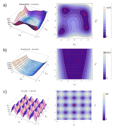
In the following, we give a short description of the optimization algorithms that are implemented in MAGIX using the analytic Himmelblau-, Rosenbrock-, and Rastrigin functions (Fig. 1) as test functions for demonstration, with multiple minima (Himmelblau, Rastrigin) and a very shallow minimum (Rosenbrock). The optimization problem is solved directly through these algorithms via stochastic searching without derivatives or gradient information (except for the Levenberg-Marquardt algorithm).

4.1 Levenberg–Marquardt algorithm

Figure 2: Results for the Rosenbrock function using the LM algorithm with start values $x_{1}=4.5$, $x_{2}=1.0$: The distribution of the parameter values after five function calls ($\chi^{2}=1.38\cdot 10^{-9}$) is indicated by green-yellow points. The sequence of iterations is color-coded (color bar on the lower right). Early points are denoted in dark green, points toward the end of the iteration are light yellow. The red dot denotes the global minimum of the Rosenbrock function.

The Levenberg–Marquardt algorithm (LM), Marquardt 1963 ; Nocedal & Wright 2006 ; Press et al. (2007) is a hybrid between the Gauss–Newton algorithm and the method of gradient descent. The Gauss–Newton algorithm is a method for solving non-linear least-squares problems. It is a modification of Newton’s method to find the minimum of a function, but is constrained so that it can only minimize a sum of square function values. It requires knowledge of the gradients in $\chi^{2}$ space, which can be obtained from differential steps for sufficiently smooth functions. The LM can find a minimum (possibly local) even if it starts very far from it, but the efficiency depends on the landscape of the parameters. On the other hand, for functions and starting values of parameters that are very close to the final minimum, the LM tends to be slower than Gauss–Newton. The LM is an algorithm that strongly depends on the starting values of the parameters that are to be optimized, and the user should choose the starting values very carefully. Otherwise the algorithm can easily become stuck in a side minimum of the global solution.

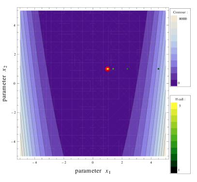
MAGIX contains a modified version of the MINPACK package implementation Garbow et al. (1980). The gradient of the $\chi^{2}$ function is calculated in a parallel environment using OpenMP. Furthermore, the user can define the variation $var$ used for the gradient determination. Because MAGIX cannot determine the gradient analytically, MAGIX has to use a numerical approximation: $(\partial/\partial x_{i})f(\@vec{x})=(f(x_{i}+h)-f(x_{i}))/h$, where the variation $h$ is defined by $h=x_{i}\cdot var$. Varying the size of the variation may be necessary if the $\chi^{2}$ function is not a smooth function and the calculation of the gradient produces awkward results. As shown in Fig. 2, the fast convergence of the LM is obvious, where the minimum is found after five (!) iterations.

4.2 Simulated annealing

Figure 3: Results for the Rastrigin function using the SA algorithm with start values $x_{1}=-1.0$, $x_{2}=-1.0$: The distribution of the parameter values after 155 function calls ($\chi^{2}=4.37\cdot 10^{-7}$) is indicated by green-yellow points. The sequence of iterations is color-coded (color bar on the lower right). Early points are denoted in dark green, points toward the end of the iteration are light yellow. The red dot denotes the global minimum of the Rastrigin function.

Simulated annealing (SA), Press et al. (2007) is a generic probabilistic computational method that is used for the problem of global optimization, i.e., to find a good approximation to the global optimum of a given function in a large parameter space. For certain problems, SA is more effective than exhaustive enumeration – provided that the goal is merely to find an acceptably good solution in a fixed amount of time, rather than the best possible solution.

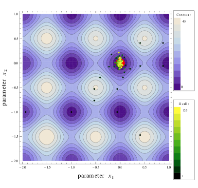
In comparison to the LM, SA is more robust. Its result does not depend so much on the neighborhood of the starting point. The LM searches for the highest (negative) gradient and stops when it detects a local minimum. In contrast, SA can check if the gradient around a local minimum is flat (low perturbation), in which case it will continue to find a better minimum, i.e., a lower value than the one found before. In Fig. 3, the SA algorithm is able to find the global minimum of the Rastrigin function at $x_{1}=0$ and $x_{2}=0$ although it starts in a local minimum at $x_{1}=-1$ and $x_{2}=-1$.

The name and inspiration of this algorithm come from the process of annealing in metallurgy. This technique involves heating and controlled cooling of a material, with the aim to gradually increase the size of its crystals and reduce their defects. The heat provides energy and causes the atoms to move from their initial position (which was a local minimum of internal energy) and wander randomly through states of higher energy. Then, a slow cooling gives them more chances of finding configurations of lower internal energy than the initial one.

By analogy to the physical process, each step of SA replaces the current solution by a random nearby solution. This nearby solution is chosen with a probability that depends both on the difference between the corresponding function values and on a global temperature, $T$. The temperature $T$ is gradually decreased (multiplied by the temperature reduction coefficient, $k<1$) during the process.

The dependency of the temperature difference between two subsequent steps is such that the solution changes almost randomly when $T$ is high, but it is modified increasingly toward lower values as $T$ becomes zero. Allowing for increasing values prevents the method from becoming stuck at local minima – which can happen with gradient methods such as the LM. Subsequent points of the SA algorithm follow a perpendicular direction.

MAGIX uses a partially parallelized implementation of the scipy algorithm using OpenMP.

4.3 Particle swarm optimization

Figure 4: Results for the Rosenbrock function using the PSO algorithm: The distribution of the parameter values after 819 function calls ($\chi^{2}=2.31\cdot 10^{-5}$) is indicated by green-yellow points. The sequence of iterations is color-coded (color bar on the lower right). Early points are denoted in dark green, points toward the end of the iteration are light yellow. The red dot denotes the global minimum of the Rosenbrock function. (The clustering of the function calls right above the global minimum is caused by the very flat gradient of the Rosenbrock function in this area.)

The particle swarm optimization (PSO) algorithm implemented in MAGIX is a hybrid Fan & Zahara (2007) between a particle swarm optimization algorithm Kennedy & Eberhart (1995) and a Nelder–Mead simplex search method Nelder & Mead (1965). The PSO optimizes a problem by iteratively trying to improve a candidate solution according to some measure of quality; the particles are sent toward a better solution flying so much faster according to the technique’s performance in previous step. The Nelder–Mead technique or downhill simplex search method is a traditional technique for the direct search of function minima; it is easy to use, does not need calculation of derivatives and therefore can converge even to non-stationary solutions.

Both techniques have been modified by Fan and Zahara Fan & Zahara (2007) and their combination is the hybrid algorithm that is available in MAGIX. The PSO algorithm performs a kind of heuristics: It starts from an initial random population of particles and searches in the neighborhood for a global optimum. The particles with the best-fit function values are updated with the simplex method, while the particles with the poorest function values are updated with the PSO.

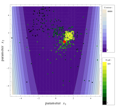
The whole procedure prevents the algorithm from being trapped locally and at the same time allows it to find the global minimum. It repeats itself until a termination criterion or the maximum number of iterations is reached. The iteration shown in Fig. 4 stops after 819 function calls because the value of $\chi^{2}$ dropped below the limit of $\chi^{2}=9\cdot 10^{-5}$. The corresponding parameter values are $x_{1}=0.9954$, and $x_{2}=0.9907$ instead of $x_{1}=1$ and $x_{2}=1$. Reducing the limit of the $\chi^{2}$ value would lead to a better description of the global minimum but it would require more function calls. The algorithm implemented in MAGIX is parallelized using OpenMP.

4.4 Bees algorithm

Figure 5: Results for the Himmelblau function using the bees algorithm: The distribution of the parameter values after 1477 function calls is indicated by green-yellow points. The sequence of iterations is color-coded (color bar on the lower right). Early points are denoted in dark green, points toward the end of the iteration are light yellow. The red dots denote the four global minima of the Himmelblau function.

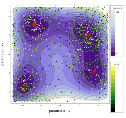
The bees algorithm Pham et al. (2005) is a swarm algorithm that performs a kind of neighborhood search combined with a random search (see, Fig. 5). This name was given to the algorithm because it tries to mimic the collection of nutriments by honey bees, in that there is always a part of the population that performs the role of scouts, traveling far away in random directions to detect new nutrition sources.

The algorithm starts with an initial set of parameter vectors (a collection of particles or scout bees, i.e., the hive of bees), randomly selected and such that it spreads throughout the entire parameter space. After the fitness of each bee is evaluated in terms of the quality ranking it just visited, the bees with the highest fitness visit the neighborhoods of the sites they currently are at. Of the remaining bees some are sent away to random sites and some are sent to search in the neighborhood of the very best sites as well (so that there are more bees searching for food in places where it is more probable to find nutrition sources). At the end of the step, the fitness of each visited site is evaluated, and the bees who just visited them move away or search in the closer vicinity of the best sites. The result is that the bees algorithm finds areas of local minima, see Fig. 5.

4.5 Genetic algorithm

Figure 6: Results for the Rosenbrock function using the GA: The distribution of the parameter values after 1112 function calls ($\chi^{2}=9.33\cdot 10^{-3}$) is indicated by green-yellow points, where the dark green points indicate function calls that are made at the beginning of the fit process and light yellow points represent function calls at the end of the fit process. The red dot denotes the global minimum of the Rosenbrock function.

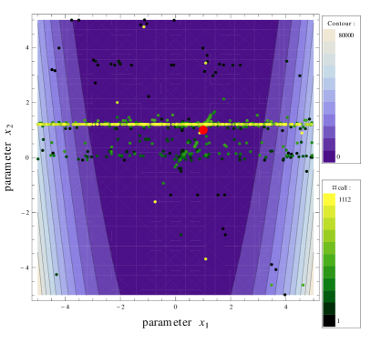
The genetic algorithm (GA) is a probabilistic search algorithm that mimics the process of natural evolution. It iteratively transforms a set of parameter vectors (population), each with an associated fitness value, into a new population of objects.

The procedure takes place using the Darwinian principle of natural selection, with operations that are patterned after naturally occurring genetic operations such as recombination and mutation. Recombination is the joined process of reproduction and crossover, i.e., mixing the genetic matter (parameter values) of the parents (parameter vector) Whitley (1994). Mutation is the complete disappearance of specific genetic material and its transformation to a completely different material; this happens especially in combinations of genetic material (parameter sets) that does not fit.

The evolution starts from a randomly selected population (of parameter sets) and proceeds in evolutionary generations (stages/iteration steps). When a generation step is completed, the fitness of all members of the population is evaluated. Then a number of parameter sets is stochastically selected for modification; the fittest members are more likely to be kept unmodified. The rest of the population members are modified; the modifications they go through are more intense because they are fit. The modified and unmodified parameter sets make up the new population whose fitness will be evaluated at the end of the step Herrera et al. (1998, 2005) (see, Fig. 6).

4.6 Nested sampling

Figure 7: Principle of the NS algorithm (taken from Skilling and MacKay (2012)): The upper part of both panels describes a contour plot of a likelihood function $\mathcal{L}(\theta)$. Left panel a): Each point $\theta$ within parameter space $\wp$ defined by the parameter ranges of $\theta_{1}$ and $\theta_{2}$ is associated with the volume that would be enclosed by the contour $L=\mathcal{L}(\theta)$. ($L(x)$ is the contour value such that the volume enclosed is $x$). If the points $\theta$ are uniformly distributed under the prior probability distribution (prior), all these volumes ($x$-values) are uniformly distributed between 0 and 1. Right panel b): Using a Markov chain method, the NS algorithm takes a point (purple dot) from $\wp$ satisfying $L\geq L(x_{1})$. Inserting the new point into this distribution, we can find the highest $x$-value $x_{2}$ used for the next iteration.

The nested sampling (NS) Skilling (2006); Feroz & Hobson (2008) algorithm included in MAGIX is a combination of a Monte Carlo method and Bayesian statistics Sivia & Skilling 2006 . The Monte Carlo methods are a family of computational algorithms that perform repeated random sampling and compute the results for every sample. The Bayesian statistics is a statistical inference technique, i.e., it attempts to draw conclusions from data subject to random variation. In particular, the Bayesian inference calculates the probability that a hypothesis is true, i.e., how probable it is that the newly calculated value of a parameter is closer to the real one (the value that best fits experimental data); if it is more probable than the previously calculated, then the parameter value is updated.

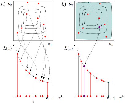
The principle of the NS algorithm is illustrated in Fig. 7: The Bayesian approach is used to obtain a set of physical parameters $\Theta=(\theta_{1};\theta_{2},\ldots,\theta_{n})$ that attempts to describe the experimental data. The Bayesian analysis is assumed to incorporate the prior knowledge with a given set of current observations to make statistical inferences. The prior information $\pi(\Theta)$ can come from observational data or from previous experiments. Bayes theorem states that the posterior probability distribution of the model parameters is given by

$${\rm Pr}(\Theta)=\frac{\mathcal{L}(\Theta)\,\pi(\Theta)}{Z},$$ (1)

where Pr$(\Theta)$ is the posterior probability distribution of the model parameters, $\mathcal{L}(\Theta)$ is the likelihood of the data for the given model and its parameters, $\pi(\Theta)$ is a prior information, and $Z$ is Bayesian evidence. The Bayesian evidence is the average likelihood of the model in parameter space. It is given by the following integral over the $n$-dimensional space:

$$Z=\int\mathcal{L}(\Theta)\pi(\Theta)\,d\Theta.$$ (2)

The NS algorithm transforms the integral (2) to the single dimension by re-parametrization to a new linear variable – a prior volume $X$. The volume of parameter space can be divided into elements $dX=\pi(\Theta)d\Theta$. The prior volume $X$ can be accumulated from its elements $dX$ in any order, so we construct it as a function of decreasing likelihood:

$$X(\lambda)=\int_{\mathcal{L}(\Theta)>\lambda}\pi(\Theta)\,d\Theta.$$ (3)

That means that the cumulative prior volume covers all likelihood values exceeding $\lambda$. As $\lambda$ increases, the enclosed volume $X$ decreases from $X(0)=1$ to $X(1)=0$. If the prior information $\pi(\Theta)$ is uniformly distributed in the parameter space, equation (2) for the evidence transforms into

$$Z=\int_{0}^{1}\mathcal{L}(X)\,dX.$$ (4)

One can calculate the partial likelihood as $L_{i}=\mathcal{L}(X_{i})$, where the $X_{i}$ is a sequence of decreasing values, such that

$$0<X_{m}<\ldots<X_{2}<X_{1}<1.$$ (5)

MAGIX uses the trapezoid rule to approximate the evidence

$$Z=\sum_{i=1}^{m}Z_{i},\quad{\rm where}\quad Z_{i}=L_{i}\,\frac{X_{i-1}-X_{i+1}}{2}.$$ (6)

The NS algorithm is targeted at calculating Bayesian evidence, but it assists in obtaining a posterior sample of points from which one can estimate uncertainties of parameter values. The prior volume $X_{i}$, which corresponds to the likelihood contour $L_{i}$, is usually evaluated with a random number generator.

The actual algorithm is based on the Markov chain Monte Carlo (MCMC) methods Press et al. (2007); Gilks et al. 1996 ; Diaconis 2009 . Those are a family of algorithms that sample from probability distributions, with the aim to construct a (Markov) chain with the desired distribution (a distribution with the desired properties) as the equilibrium distribution. The quality (how well the parameter sets fit the data) of the sample is a monotonically increasing function of the number of steps (see, Fig. 7).

Figure 8: Results for the Himmelblau function using the NS algorithm: The distribution of the parameter values after 2599 function calls is indicated by green-yellow points, where the dark green points indicate function calls which are made at the beginning of the fit process and light yellow points represent function calls at the end of the fit process. The red dots denote the four minima of the Himmelblau function.

Figure 9: Results for the Himmelblau function using the INS algorithm: Left panel: The distribution of the parameter values after 251 function calls is indicated by green-yellow points, where the dark green points indicate function calls that are made at the beginning of the fit process and light yellow points represent function calls at the end of the fit process. The red dots denote the four minima of the Himmelblau function. Right panel: Posterior weights of points after the NS process.

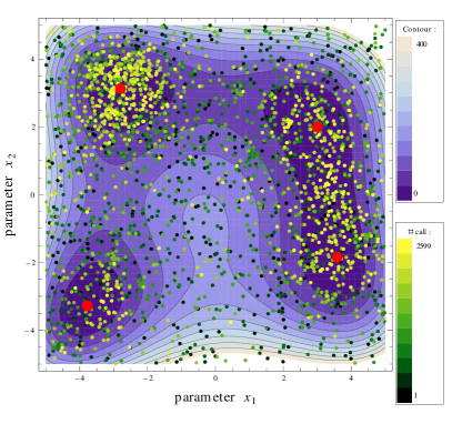
An MCMC algorithm is used to reduce the dimensionality of the parameter space through integration. The Bayesian approach to this technique allows one not only to find multiple solutions, but also to define proportional weights of parameter values and to evaluate the Bayesian evidence. The NS algorithm included in MAGIX requires fewer samples than standard MCMC methods Feroz & Hobson (2008) while also providing posterior probabilities for each one of the best parameter vectors. The NS algorithm has the following advantages: It is a non-derivative method and investigates the landscape of optimization function. Additionally, it can find multiple minima. On the other hand, the algorithm does not converge to a global minimum and depends strongly on the random number generator. The results for the Himmelblau function, shown in Fig. 8, are similar to the results of the bees algorithm. Both algorithms can be used to explore the landscape of the $\chi^{2}$ distribution and for finding areas of global minima. The implementation of the algorithm included in MAGIX is parallelized using OpenMP.

4.7 Interval nested sampling algorithm

The Interval Nested Sampling (INS) algorithm (developed by I. Bernst) included in MAGIX is an implementation of the branch-and-bound algorithm Ichida & Fujii (1979) to find the next prior volume $X_{i}$. The algorithm is based on the NS algorithm (§4.6) and uses an interval method for the definition of a next part of the prior volume. The main principle of the interval method is a division of the parameter space into interval boxes and an estimation of the optimization function value over the boxes. The estimate is called inclusion function and can be calculated by various methods. The centered form of inclusion with slopes is used in the current version of the INS algorithm Krawczyk (1985). The interval method assists in finding the next prior volume $X_{i}$ by determining the ratio of the volume of the working interval box $Z_{i}$ to the whole volume $Z$ of the parameter space. Posterior weights of points after the NS process are calculated using the Bayes theorem (see, Fig. 9):

$$w_{i}=\frac{Z_{i}}{Z}.$$ (7)

Using the sequence of posterior samples of parameter vectors we are able to determine the reliability of model parameters such as standard deviations or to construct posterior distributions of parameter values. The mean value $\mu(\theta_{j})$ of each model parameter $\theta_{j}$, $j=(1,\ldots,n)$ and its standard deviation $\sigma(\theta_{j})$ are given as

$$\mu(\theta_{j})=\sum_{i=1}^{k}w_{i}\,\theta_{j}$$ (8)

and

$$\sigma(\theta_{j})=\sqrt{\sum_{i=1}^{k}w_{i}\left(\theta_{j}-\mu(\theta_{j})\right)^{2}},$$ (9)

where $k$ indicates the number of points in the sample. The INS algorithm is capable of handling multi-modality of the optimization function, phase transitions, and strong correlations between model parameters. As shown in Fig. 9, the Interval Nested Sampling algorithm requires fewer function calls than other global optimizers. Additionally, it is used to determine the confidence intervals of parameters, which is described in the next section.

4.8 Error estimation

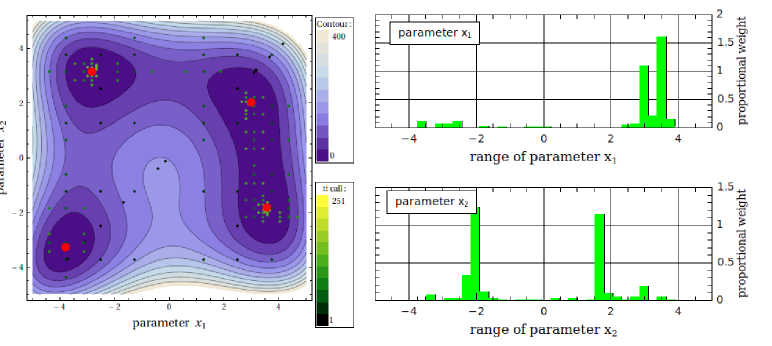
MAGIX provides an error estimation for each single parameter at the point of minimum. A schematic diagram of the error estimation module is shown in Fig. 10: After some optimization procedure MAGIX determines a point of minimum. The input values for the error estimation are given by the point of minimum and the parameter space. To determine the error of a parameter $\theta_{j}$ at the minimum, MAGIX varies this parameter within the given parameter range, while the other parameters are kept constant. The INS algorithm is applied and returns a set of parameter values with proportional weights and the logarithm of the Bayesian evidence for parameter $\theta_{j}$ for a sequence of parameter values distributed over the whole parameter space. If the distribution of parameter values has only one minimum, Eqn. (8) - (9) can be applied to calculate the mean value and the standard deviation. Sometimes there are several minima in the sequence, hence these formulas cannot be used directly because the resulting estimation of the mean value and standard deviation produces meaningless results (see Figs. 9 and  11).

Figure 10: Schematic diagram of error estimation module of MAGIX.

Figure 11: Distribution of parameter values with several minima where a direct application of Eqn. (8) - (9) is not possible. (Here, $\mu(\theta_{j})$ indicates the mean value $\mu(\theta_{j})$, $\sigma(\theta_{j})$ is the standard deviation $\sigma(\theta_{j})$, and “min” represents the value of the parameter $\theta_{j}$ of the best-fit result).

Figure 12: Schematic diagram of error estimation module of MAGIX. (Here, $\mu(\theta_{j})$ indicates the mean value $\mu(\theta_{j})$, $\sigma(\theta_{j})$ represents the standard deviation $\sigma(\theta_{j})$, and “min” the value of the parameter $\theta_{j}$ of the best-fit result).

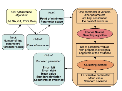
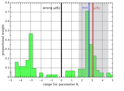
We are interested in the uncertainty around the considered minimum. Therefore, we need to estimate the mean value and the standard deviation in the minimum. This is done using a clustering method:

• Calculate the distances from the minimum to all points of the sample.

• Sort the points depending on their distances (ascending order).

• Select the points with a function value lower than the $\chi^{2}$ boundaries for the 99 percent confidence region $\Delta\chi^{2}_{\alpha,n}$ ($\alpha$ = 0.99).

Finally, the new sample of $m$ points ($m<k$) is distributed around the minimum point (Fig. 11, gray box) and the mean value of the parameter $\theta_{j}$ is calculated as follows:

$$\mu\left(\theta_{j}\right)=\frac{\sum_{i=1}^{m}w_{i}\theta_{j}}{\sum_{i=1}^{m}w_{i}}.$$ (10)

In Bayesian statistics one usually applies a credible interval (or Bayesian confidence interval) to the parameter value. For a single parameter and a sample of points that can be summarized in a single sufficient statistic, it can be shown Jaynes (1976) that the credible interval and the confidence interval coincide if the unknown parameter is a location parameter (i.e., the forward probability function has the form $Pr$($\theta_{i}|\mu(\theta_{i})$) = $f$($\theta-\mu$) ) with a uniform prior distribution. Hence credible intervals in our case are analogous to confidence intervals in frequentist statistics. Using the mean value $\mu(\theta_{j})$ and the standard deviation $\sigma(\theta_{j})$, the 3$\sigma$ confidence interval of the parameter $\theta_{j}$ is given by

$$Pr(\mu(\theta_{j})-\sigma(\theta_{j})<\theta_{j}<\mu(\theta_{j})+\sigma(\theta_{j}))\approx 0.99.$$ (11)

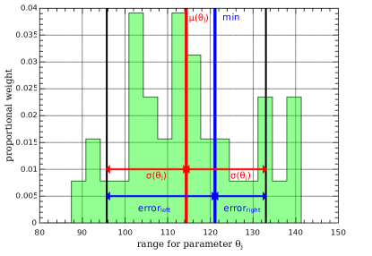
In Fig. 12 the example of a histogram of distribution of parameter values after error estimation is shown. Hence for the parameter value at the point of minimum (using the error left and the error right),

$$Pr(\theta_{i}({\rm min})-{\rm error}_{\rm left}<\theta_{j}<\theta_{i}({\rm min})+{\rm error}_{\rm right})\approx 0.99.$$ (12)

The Bayesian evidence usually plays an important role in model selection but in parameter estimation the evidence factor is ignored because it is an integrated value over the whole parameter space. The INS algorithm calculates the logarithm of the evidence and can be used to estimate the quality of the fitting procedure. A high absolute value of the evidence logarithm indicates a big uncertainty of the parameters.

4.9 Which algorithm should be used?

Figure 13: Results for the Rosenbrock function using an algorithm chain: Left panel: The distribution of the parameter values for the bees algorithm (green-yellow points, where the dark green points indicate function calls that are made at the beginning of the fit process and light yellow points represent function calls at the end of the fit process) and for the following simulated annealing algorithm (white points). The red dot indicates the global minimum of the Rosenbrock function. Right panel: Posterior weights of points after the NS process used by the error estimation module.

In principle, it is impossible to answer the question which algorithm is best. All algorithms included in MAGIX try to find the global minimum of the $\chi^{2}$ function, which depends on the observational data, on the external model, on the free and fixed parameters, and on the ranges for each free parameter. Every algorithm has a different strategy for finding the minimum of the $\chi^{2}$ function. Whether the strategy is successful depends on the $\chi^{2}$ function and many other conditions. For example, the bees algorithm requires a huge computational effort, but this algorithm explores the whole landscape of the $\chi^{2}$ function within the given ranges. It gives a good overview of the landscape of the problem and can in principle find even minima in narrow valleys. On the other hand the computational effort is heavy, and the algorithm is inefficient if computing the external model requires more than a few seconds. Here, the computation time of an algorithm depends on the number of function calls for each iteration, the computation time of the external model program, the possibility of executing the external model program more than once on the same machine at the same time and on the size of the parameter space. Other swarm algorithms such as the particle swarm or NS algorithms might be better if the $\chi^{2}$ function has a smoother shape. For example, the particle swarm algorithm included in MAGIX makes use of a Nelder–Mead simplex search method, which accelerates the whole computation if the $\chi^{2}$ function has no narrow valleys, i.e, the $\chi^{2}$ function does not change drastically when one or more parameters are varied.

Table 1: Total cost (in function evaluations) for each test function for each global optimization algorithm.

algorithm	Rastrigin	Rosenbrock	Himmelblau
name	function	function	function
	$\chi^{2}_{\rm limit}=1$	$\chi^{2}_{\rm limit}=4\cdot 10^{-3}$	$\chi^{2}_{\rm limit}=5\cdot 10^{-4}$
Bees	$1220$	$14491$	$101664$
PSO	$1317$	$535$	$770$
Genetic	$241$	$533$	$1626$
NS	$4230$	$5080$	$8720$
INS	$20$	$1144$	$168$

In Table 12 the total cost (in function evaluations) for each test function (Rastrigin, Rosenbrock, and Himmelblau function) for each global optimization algorithm is shown. As mentioned above, the total cost of an algorithm, i.e., the number of function evaluations depends strongly on many parameters. Therefore, Table 12 can give only a very rough overview of the efficiency for each algorithm. For example, the INS algorithm is quite efficient in finding the global minimum of the Rastrigin function but less efficient in finding the global minimum of the Rosenbrock function.

In general, the global optimization algorithms are more efficient in finding the areas of global minima. But they are less efficient in finding the exact properties of the global minima. For that purpose, local optimizers, such as the LM or SA are much more efficient. The combination of different algorithms is the best strategy to find the complete description of the experimental data.

4.10 Algorithm chain

Table 2: Best parameter set with the corresponding confidence intervals ($\chi^{2}=2.5576\cdot 10^{-5}$) after applying an algorithm chain.

parameter	value at	error	error	log
name	minimum	left	right	(evidence)
$x_{1}$	$0.9954$	$3.43\cdot 10^{-2}$	$2.85\cdot 10^{-2}$	$-3.309$
$x_{2}$	$0.9905$	$7.38\cdot 10^{-2}$	$8.21\cdot 10^{-2}$	$-2.846$

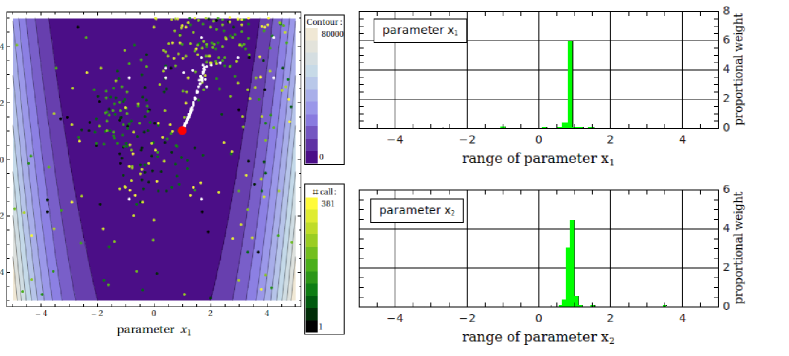
Therefore, MAGIX includes the possibility to send the results of the optimization process performed by one algorithm to another optimization loop through some different algorithm. As mentioned above, the SA as well as the LM algorithm require starting values of the parameters that are optimized, i.e., the user has to find a good fit by hand before applying these algorithms produces useful results. Often, the location of the minimum can be guessed with sufficient accuracy to give good starting values, but sometimes one is completely in the dark. Using an algorithm chain, the user can first apply one of the swarm algorithms, e.g., the bees or NS algorithm, to determine the starting values for the subsequent local optimization algorithm using SA or the LM algorithm. As shown in Fig. 13, we used an algorithm chain to determine the global minimum of the Rosenbrock function where we first applied the bees algorithm to explore the landscape of the problem. Using the best result of the bees algorithm (the parameter set that corresponds to the lowest $\chi^{2}$ value, here $x_{1}=1.7044$ and $x_{2}=2.8679$) as starting point for the SA algorithm, we find the global minimum of the Rosenbrock function. MAGIX does not only allow one to use the best but also the second best etc. result of a swarm algorithm as starting values for other algorithms. Therefore, we are able to find multiple minima of models that behave as the Himmelblau function.

To determine the confidence intervals for the parameters that are optimized, the user has to set the error estimation algorithm as the last algorithm of the algorithm chain. The confidence intervals for the parameters that are used in the example shown in Fig. 13 are given in Table 13. The upper right panel of Fig. 13 shows the probability for a minimum along the $x_{1}$ axis holding parameter $x_{2}$ fixed at $x_{2}=0.9905$. The lower right panel of Fig. 13 shows the probability for a minimum along the $x_{2}$ axis holding parameter $x_{1}$ fixed at $x_{1}=0.9954$. These two panels clearly show that there is only one minimum within the given parameter range.

5 Examples

Figure 14: Fit of H₂O⁺ using myXCLASS and MAGIX. In blue one specific component depicts the intrinsic hyperfine structure of the lines, while the green bars locate the positions of the velocity components.

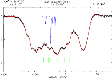
The first astrophysical application of MAGIX was fitting Herschel/HIFI spectra of an ortho-H₂O⁺ line in Band 4b with myXCLASS, in particular absorption lines toward SgrB2(M) from the HEXOS GT KP Schilke et al. (2010). Here, the line shape is determined by the hyperfine structure and the velocity structure, resulting in a complicated pattern. The fit was performed using the LM algorithm. As can be seen in Fig. 14, the match is convincing, but questions about the uniqueness of the fit and confidence intervals for the free parameters, about 100 in this case do arise.

Figure 15: Fit of ortho H₂O⁺ ground state lines in HIFI bands a) 4b and b) 5a toward SgrB2(M) with myXCLASS using an algorithm chain consisting of the genetic, the SA, and the error estimation algorithm. Owing to the high number of free parameters (78) it is not possible to show the distribution of the parameter values as in Figs. 2 - Fig. 13.

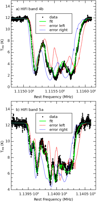
Additionally, we fit HIFI bands 4b and 5a toward SgrB2(M) Schilke et al. (2010) with myXCLASS, simultaneously using an algorithm chain starting with the genetic algorithm and 78 free parameters (we used 26 velocity components where each component has three free parameters.). Here, we used the parameter values of the best fit-result of the genetic algorithm as starting values for the SA. At the end of the algorithm chain, we applied the error estimation algorithm to determine the left and right error for each optimized parameter. The final result is shown in Fig. 15, where the dashed red (blue) lines indicate a model where we reduced (increase) the free parameter values of the best fit by the left (right) error of each free parameter. Clearly, we achieve an excellent description of the absorption lines and quantify the uncertainty of the model. In contrast to the previous fit shown in Fig. 14, where only one data set was fitted, we defined no starting values but only ranges for each free parameter and fitted two bands simultaneously.

6 Conclusions

The MAGIX package presented in this paper is a very helpful tool for modeling physical and chemical data using an arbitrary external model program. It represents a highly flexible toolbox where in principle any theoretical external model program can be plugged in. Thus, MAGIX can be used to optimize the description of even non-astrophysical data. Furthermore, MAGIX is able to explore the landscape of the $\chi^{2}$ function without the knowledge of starting values and can calculate probabilities for the occurrence of minima. Therefore, MAGIX can find multiple minima and give information about confidence intervals for the parameters. Additionally, the MAGIX package contains the possibility to combine algorithms in a so-called algorithm chain and make use of the advantages of the different algorithms included in the package. If the external model program fulfills certain requirements, MAGIX can run in a parallel mode to speed up the computation.