Precise Measurement of the Radial Baryon Acoustic Oscillation Scales in Galaxy Redshift Surveys

Abstract

In this paper we present a new method to extract cosmological parameters using the radial scale of the Baryon Acoustic Oscillations as a standard ruler in deep galaxy surveys. The method consists in an empirical parametrization of the radial 2-point correlation function, which provides a robust and precise extraction of the sound horizon scale at the baryon drag epoch. Moreover, it uses data from galaxy surveys in a manner that is fully cosmology independent and therefore, unbiased. A study of the main systematic errors and the validation of the method in cosmological simulations are also presented, showing that the measurement is limited only by cosmic variance. We then study the full information contained in the Baryon Acoustic Oscillations, obtaining that the combination of the radial and angular determinations of this scale is a very sensitive probe of cosmological parameters, able to set strong constraints on the dark energy properties, even without combining it with any other probe. We compare the results obtained using this method with those from more traditional approaches, showing that the sensitivity to the cosmological parameters is of the same order, while the measurements use only observable quantities and are fully cosmology independent.

1 Introduction

Finding the physical origin of the accelerated expansion of the Universe is one of the most important scientific problems of our time, and is driving important advances in XXIst century cosmology. Several observational probes to study the nature of the mysterious dark energy, which powers that expansion, have been proposed. Among them, the measurement of the scale of the Baryon Acoustic Oscillations (BAO) in the galaxy power spectrum as a function of redshift is one of the most robust, since it is insensitive to systematic uncertainties related to the astrophysical properties of the galaxies. Moreover, it provides information about dark energy from two different sources: the angular diameter distance, through the measurement of the BAO scale in the angular distribution of galaxies, and the Hubble parameter, through the measurement of the BAO scale in the radial distribution of galaxies.

There are some measurements of the BAO scale in the purely radial direction (Gaztañaga et al., 2009; Kazin et al., 2010; Xu et al., 2013), but most of them use mainly the monopole of the 3-D correlation function (Eisenstein et al., 2005; Hütsi, 2006a, b; Percival et al., 2007; Padmanabhan et al., 2007; Okumura et al., 2008; Sánchez et al., 2009; Anderson et al., 2012). This has been the traditional way of determining the BAO scale, trying to optimize the sensitivity when the number of galaxies in the survey is not very high, paying the price of introducing model dependence in the measurement through the use of a fiducial model. However, the new galaxy surveys which are already taking data or those proposed for the future do not suffer from this problem and new and more robust methods can be used.

In this paper we propose a new method to extract the evolution of the radial BAO scale with the redshift, and explain how to use it as a standard ruler to determine cosmological parameters. We use data from galaxy surveys in a manner that is fully cosmology independent, since only observable quantities are used in the analysis and therefore, results are unbiased. A method based on the same idea for the measurement of the angular BAO scale was described in Sánchez et al. (2011) and provided the measurement of the angular BAO scale presented in Carnero et al. (2012). Here we present how to extract the radial BAO scale using a similar approach.

The method is designed to be used as a strict standard ruler, and provides the radial BAO scale as a function of the redshift, but we do not intend to give a full description of the radial correlation function. This approach is more robust against systematic effects, and in fact we demonstrate that the measurement is only limited by cosmic variance, since the associated systematic errors are much smaller than the purely statistical errors.

2 Galaxy Clustering and Observables

One of the main statistical probes of the properties of the matter distribution in the Universe is the 2-point correlation function, $\xi(r)$, which is defined as the excess joint probability that two point sources (e.g. galaxies) are found in two volume elements $dV_{1}dV_{2}$ separated by a distance $r$ compared to a homogeneous Poisson distribution (Peebles, 1980). If the fluctuations on the matter density field are Gaussian, this function contains all the information about the large scale structure of the Universe.

However, what is observationally accesible is the distribution of galaxies in angle-redshift space, not directly the matter distribution in real space. For each galaxy we determine its angular position in the sky and its redshift. To obtain $\xi(r)$ we need to convert the measured redshift to a comoving distance, for which a cosmological model is needed. Therefore, the 3-D correlation function is not observable in a cosmology independent way for a given galaxy survey. Moreover, the observational techniques to obtain the angular position in the sky and the redshift are completely different and independent. Consequently, if we want to keep the measurement completely free of any theoretical interpretation, we should measure, on the one hand, the angular correlation function as a function of the angular separation of galaxy pairs, and on the other hand, the radial correlation function as a function of the redshift separation of galaxy pairs, and then extract the BAO scale from each function. Both of them are defined in complete analogy with the 3-D function, as the excess of probability with respect to a homogeneous Poisson distribution, and both are observable in a cosmology independent way, providing, together, information about the full 3-D large scale structure that can be described in any cosmological model. These aspects have been recently pointed out in Bonvin & Durrer (2011), and here we present a practical implementation of a cosmology independent measurement, in this case for the radial BAO scale.

Several effects must be taken into account when the large scale structure of the Universe is studied from galaxy surveys, like bias, redshift space distortions and non-linear corrections. In this paper we take all of them into account, both in the theoretical calculations and in the observational analysis. For this particular measurement, the influence of the non-linear effects is relatively small, since we are analyzing large scales, around the BAO scale. Also the influence of bias is small, because the analysis method is designed to minimize its impact on the final result. However, redshift space distortions are very important, since we are measuring along the line of sight.

3 The Sound Horizon Scale

The BAO are a consequence of the competition between gravitational attraction and gas pressure in the primordial plasma, which produced sound waves. Differences in density created by these sound waves leave a relic signal in the statistical distribution of matter in the Universe, defining a preferred scale, the sound horizon scale at the baryon drag epoch, which is a robust standard ruler from which the expansion history of the Universe can be inferred. The BAO scale is very large, $\sim 100$ Mpc/h, which poses an important challenge for observations, since surveys must cover large volumes to map such a distance. However, the very large scale of BAO also has certain advantages, because structure formation at these scales is rather well understood, and details about the description of galaxy formation and astrophysics do not compromise the accurate measurements of the standard ruler. In practice, the strength of the BAO standard ruler method relies on the potential to relate the position of the acoustic peak in the correlation function of galaxies to the sound horizon scale at decoupling.

The current measurements of the BAO scale typically use the spherically symmetric monopole contribution of the 3-D correlation function. This is a mixture of the angular and radial scales, and therefore, does not contain all the information that can be extracted from the data samples. On top of that, all analyses have been done using what is usually called a “fiducial model” in order to determine distances. Rather than full tests of the cosmology, they should be understood as precision measurements within the context of the standard $\Lambda$CDM cosmological model. Considering this way of analyzing data, what the current results have achieved is a strong confirmation of the consistency of the current data with the standard $\Lambda$CDM model, but the analysis strategy is very limited if one wants to test other non-FLRW cosmological models against data, or at least, the whole analysis must be repeated from the very begining for every cosmological model one tries to test.

On the other hand, if both the angular and the radial BAO scales are determined, which in principle is already possible with current data sets, the cosmological constraints that can be set using only the BAO scale are much stronger than the current values, since the radial and angular scales are sensitive to cosmological parameters in quite different ways, breaking degeneracies and allowing a very precise determination when combined.

4 Method to Measure the Radial BAO Scale

The method we propose relies on a parametrization of the radial correlation function which allows extracting the radial BAO scale with precision. It is based on a similar approach previously proposed for the angular correlation function (Sánchez et al., 2011). The suggested parametrization was inspired by the application of the Kaiser effect to the shape we used for the angular correlation function.

It is important to remark that the calculations we perform to check the goodness of the parametrization do include redshift space distortions using the Kaiser description (Kaiser, 1987) and also non-linearities using the RPT approach (Crocce & Scoccimarro, 2006), and we expect the result to be correct for large scales, where the neglected effects (fingers of god, mode-mode coupling) are very small. We have used a bias parameter $b=1$ throughout the calculation. The possible influence of bias is studied in the systematic errors section. We use the linear power spectrum from CAMB (Lewis et al., 2000), on top of which non-linearities and redshift space distortions are then included.

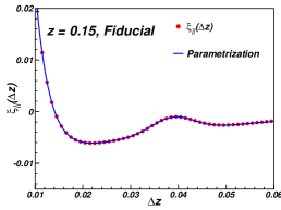
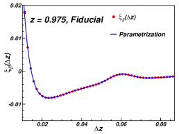
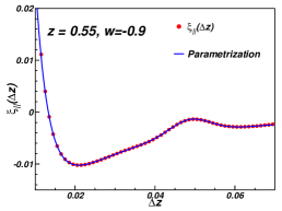
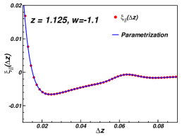
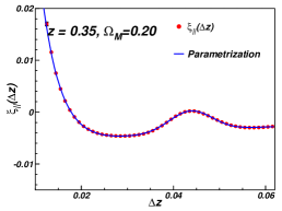
Figure 1: Some examples of the description of the different cosmological models by the proposed parametrization. Models do include redshift space distortions and non-linearities using the RPT scheme. The parametrization is a very good description of all models at all redshifts, even if the considered errors are much smaller than the cosmic variance for the full sky. Errors are smaller than the dot size. We have used this level of precision to ensure that the systematic errors associated to the theory (non-linearities, bias) are small.

The full recipe to obtain the radial BAO scale as a function of redshift for a galaxy survey is as follows:

1. Divide the full galaxy sample in redshift bins.

2. Divide each redshift bin in angular pixels.

3. Compute the radial correlation function by stacking galaxy pairs in each angular pixel, but do not mix galaxies in different angular pixels.

4. Parametrize the correlation function using the expression:

   $$\xi_{\parallel}(\Delta z)=A+Be^{-C\Delta z}-De^{-E\Delta z}+Fe^{-\frac{(\Delta z-\Delta z_{BAO})^{2}}{2\sigma^{2}}}$$ (1)

   and perform a fit to $\xi_{\parallel}(\Delta z)$ with free parameters $A$, $B$, $C$, $D$, $E$, $F$, $\Delta z_{BAO}$ and $\sigma$.

5. The radial BAO scale is given by the parameter $\Delta z_{BAO}$. The BAO scale as a function of the redshift is the only parameter needed to apply the standard ruler method. The cosmological interpretation of the other parameters is limited, since this is an empirical description, valid only in the neighborhood of the BAO peak.

6. Fit cosmological parameters to the evolution of $\Delta z_{BAO}$ with $z$.

In order to test the goodness of this parametrization, we have computed the radial correlation function for the 14 cosmological models described in Table 1 in a redshift range from 0.2 to 1.5, always including redshift space distortions and non-linearities as explained before. Then, we have applied the method to each model and each redshift. The parametrization describes the theory very accurately, since the values of the $\chi^{2}/ndof$ are close to 1, and the probabilities of the fit lie between 0.98 and 1.00 when the error in each point of the correlation function is arbitrarily fixed to 2% (or $\sim 10^{-5}$) for all bin widths and cosmological models. This error corresponds to a precision much better than the cosmic variance for the full sky, for all models in the full redshift range, but the parametrization is able to recover the correct radial BAO scale for the 14 cosmologies. We have used this level of precision because the systematic errors coming from theoretical effects (non-linearities, bias, fingers of god) only affect this method if they induce a disagreement between the models and the parametrization, giving then a wrong measurement of the BAO scale. If the description is good to this level of precision we guarantee a small contribution from these systematic effects, as will be shown in the systematic errors section below. The calculation of the realistic errors is described in the next section. Some examples of these descriptions can be seen in Figure 1.

Once we have verified the parametrization on the theoretical predictions, we are ready to apply it in more realistic environments. For this purpose, in the next section we apply this algorithm to a galaxy catalogue obtained from a N-body cosmological simulation. We will also compute the main systematic errors associated to this method.

$h$	$\Omega_{M}$	$\Omega_{b}$	$\Omega_{k}$	$w_{0}$	$w_{a}$	$n_{s}$
0.70	0.25	0.044	0.00	$-$1.00	0.0	0.95
0.68
0.72
	0.20
	0.30
		0.040
		0.048
			+0.01
			$-$0.01
				$-$0.90
				$-$1.10
					$-$0.1
					+0.1
						1.00

Table 1: Summary of the 14 cosmological models used to test the method. Where empty, the fiducial values (first line) are assumed.

5 Application to a simulated galaxy Survey

We have tested the method to recover the radial BAO scale using a large N-body simulation capable of reproducing the geometry (e.g. area, density and depth) and general features of a large galaxy survey. The simulated data were kindly provided by the MICE project team, and consisted of a distribution of dark matter particles (galaxies, from now on) with the cosmological parameters fixed to the fiducial model of Table 1. The redshift distribution of the galaxies is shown in Figure 2. The simulation covers 1/8 of the full sky (around 5000 square degrees) in the redshift range 0.1 $<$ z $<$ 1.5, and contains 55 million galaxies in the lightcone. This data was obtained from one of the largest N-body simulations completed to date , with comoving size $L_{box}=3072~{}h^{-1}$ Mpc and more than $8\times 10^{9}$ particles ($m_{p}=2.3\times 10^{11}h^{-1}M_{\odot}$). More details about this simulation can be found in Fosalba et al. (2008) and Crocce et al. (2010). The simulated catalogue contains the effect of the redshift space distortions, fundamental for the study of the radial BAO scale.

Figure 2: $N(z)$ in the used MICE catalogue. The simulation contains 55 million galaxies in the redshift range $0.1<z<1.5$. The vertical dashed lines show the limits of the redshift bins used in the analysis.

Data with similar characteristics will be obtained in future large spectroscopic surveys, such as DESpec (Abdalla et al., 2012), BigBOSS (Schlegel et al., 2011) or EUCLID (Laureijs et al., 2011).

It is important to note that the radial BAO determination needs a very large survey volume. We tried to extract the BAO peak from catalogs with smaller areas (200, 500 and 1000 sq-deg), finding a very small significance (or no detection at all) in most cases. This is due to the fact that the statistical error related to the cosmic variance is specially large for the radial correlation function, and therefore it can only be reduced by increasing the volume explored.

Thus, we have divided the simulation into 4 redshift bins. We apply the method described in the previous section for each bin and obtain the correlation functions using the Landy-Szalay estimator (Landy & Szalay, 1993). Fits are shown in Figure 3. We have used an angular pixel with of 02.5 sq-deg size, in order to retain enough number of galaxy pairs in the colliner direction. We generate the random catalogues taking into account the $N(z)$ distribution in order to obtain the correct determination of the radial correlation function. This is a very important effect, since we are measuring in the radial direction and the distributions on the redshift coordinate have a large influence in measurements. The statistical significance of the BAO observation in the first bin is very low ($\sim 1.4\sigma$) and it is consequently not considered in the cosmology analysis. Following the same approach of Sánchez et al. (2011), we have computed the statistical significance of the detection by measuring how different from zero the $F$ parameter of the fit is Eq. (1), using its statistical error.

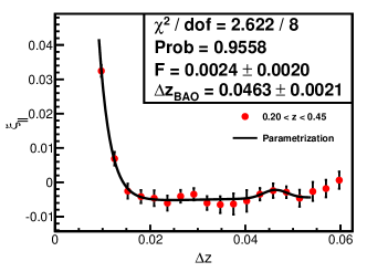
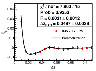
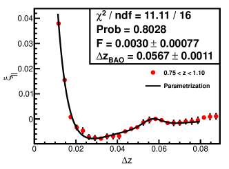
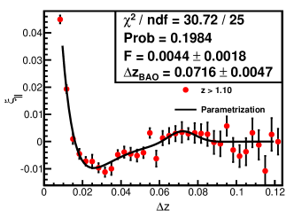
Figure 3: Radial correlation functions measured in the MICE simulation for the 4 redshift bins described in the text (dots), for an angular pixel of 0.25 sq-deg, compared with the proposed parametrization (solid line). All the fits are good. The statistical significance of the BAO detection in the first bin is very low, and it is not used to set cosmological constraints.

We have computed a theoretical estimation of the covariance matrix for the 3-D correlation function (see the Appendix A), which is then applied to the estimation of the covariance for the radial correlation function Eq. (11), taking the corresponding value for the line of sight direction. This estimate relies on the model used for the simulation, but we expect a small variation of the error with the cosmological model. In any case, to keep the method fully model independent we have validated the calculation of the covariance matrix obtaining it with an alternative method directly from the simulation, which can also be applied to any real catalogue. We have used many realizations, dividing the total area in patches of different sizes and computing the corresponding dispersions and covariance matrices. We have then obtained the error for the total area, scaling this estimates to the full area of the measurement. Both determinations agree in the region of interest for the BAO scale measurement, as is shown in Figure 4. There is a disagreement for small scales, which is coming from the incomplete description of the non-linearities in the theoretical calculation, where the mode-mode coupling effects are neglected, and from boundary effects in the realizations.

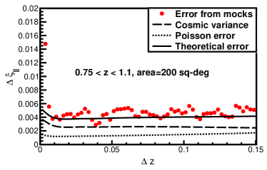
Figure 4: Comparison of the different estimates of the error in the radial correlation function are shown. The estimates are MC samples (dots) and theoretical calculation (solid line). They agree in the region of interest for the BAO analysis. The disagreement at low scales comes from the incomplete description of the non-linearities, where the mode-mode coupling effect is neglected, and from some boundary effects in the realizations, but does not affect the BAO scale measurement since it is outside the fitting region. The different contributions to the total error are shown. They come from Poisson shot noise (dotted line) and cosmic variance (dashed line). The contribution of the Poisson shot noise, proportional to the inverse of the pair counts, is not negligible.

It is important to note that the radial BAO determination needs a very large survey volume. We are not able to obtain a significant observation for the first redshift bin and the contribution to the total error of the cosmic variance and the shot noise is comparable for all the other bins, which is shown in Figure 4. As already pointed out and verified by Crocce et al. (2011), in order to obtain a correct description of the error we need to sum linearly the cosmic variance and the shot noise contribution in harmonic space. This is not surprising, since galaxy surveys are designed to have a determined and fixed galaxy density, and this fact correlates both contributions to the error.

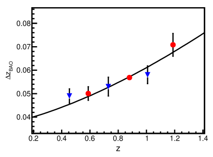
Figure 5: Measured radial BAO scale as a function of the redshift in the MICE simulation using the proposed method. Dots are the nominal bins and triangles correspond to displaced bins, and are measured only as a cross-check. All measurements are in good agreement with the theoretical prediction (solid line).

The measured values of the BAO scale as a function of the redshift can be seen in Figure 5 as dots. The results for 3 alternative bins shifted with respect to the nominal ones are also shown as triangles. These have not been used to obtain cosmology results, since they are fully correlated with the red ones and are only shown for illustration and verification of the correct behaviour of the analysis method. We have used in this analysis the center of the redshift bin to obtain the prediction of the model, although what is really observed is the average within the bin. We have verified that they are very close if the $N(z)$ distribution is smooth, as it is in this case.

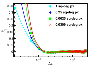
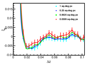
Figure 6: Effect of the angular pixel size on the radial correlation function. The finite size of the angular pixel induces a change on the slope of the correaltion function at small scales (top), but when a zoom around the position of the BAO peak is done, it is clear that this effect does not change the position of the BAO peak (bottom). The effect is shown for pixels of sizes 0.0309 (stars), 0.0625 (squares), 0.25 (crosses) and 1 (dots) square degrees. The 0.25 sq-deg pixel has been used to obtain the cosmological parameters. The change in the slope arises from the smoothing effect produced by the inclusion in the calculation of galaxy pairs which are not exactly collinear. This effect does not affect the determination of the BAO scale.

5.1 Systematic Errors

We have studied the main systematic errors that affect the determination of the radial BAO scale using this method. We have found a specific systematic effect associated to the algorithm, which is coming from the size of the angular pixel. Other systematic errors are generic and will be present in any determination of the BAO scale, namely, the influence of the non-linearities, the starting and end point of the fit to the correlation function and the possible influence of the galaxy bias in the measurement.

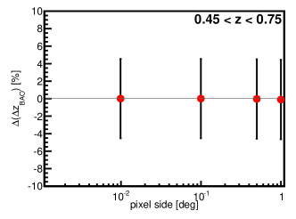
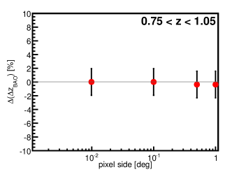
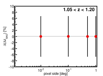
Figure 7: Variation of the radial BAO scale determination as a function of the angular pixel size for different redshifts. Results are stable, and the maximum variation is always of a few parts per mille, very well below 1%, even if the range in pixel sizes covers two orders of magnitude. The error bars indicate the size of the statistical error for the nominal pixel size of 0.25 sq-deg, including Poisson shot noise and cosmic variance, for the used simulation, that covers 1/8 of the sky.

5.1.1 Size of the Angular Pixel

One specific systematic error associated with this method is the possible influence that the size of the angular pixel has on the determination of the radial BAO scale, since it determines which galaxies are considered collinear in the analysis. The effect of different pixel sizes on the radial correlation function can be seen in Figure 6. The radial correlation function clearly changes on small scales (Figure 6, top), but this effect does not change the position of the BAO peak (Figure 6, bottom). The small scale effect comes from the smoothing of the correlation function due to the inclusion in the calculation of galaxy pairs which are not exactly collinear. For a larger angular pixel, the effect is larger. However, the scale where this effect acts is fixed by the angular pixel size, which is very far from the BAO scale, that remains, therefore, unaffected, since the parametrization is able to absorb the change in the slope of the function.

In order to quantify this influence on the determination of the BAO scale as a systematic error, we have repeated the full analysis for different pixel sizes. The obtained results are shown in Figure 7. The radial BAO scale is recovered with high precision for any angular pixel size, even for sizes as large as 1 degree, which corresponds to a range of two orders of magnitude. The associated systematic error can be estimated to be $\delta(\Delta z_{BAO})=0.20\%$, much smaller than the statistical error for the nominal pixel size of 0.25 sq-deg, which is shown as error bars.

5.1.2 Non-linearities

Also the error due to the uncertainty in the goodness of the description provided by the parametrization for different theoretical effects (non-linearities at the scale of the BAO peak) has been computed obtaining a global error of 0.10%. This was estimated in a conservative way as the difference between the $\Delta z_{BAO}$ measured using linear and non-linear $\xi_{\parallel}(\Delta z)$, for the same redshift bins of the analysis. Non-linearities are computed using the RPT formalism (Crocce & Scoccimarro, 2006), excluding mode-mode coupling, since it only affects small scales, far enough from the BAO scale. The contribution of these uncertainties to the systematic error can be estimated as $\delta(\Delta z_{BAO})=0.10\%$.

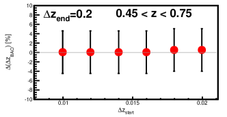
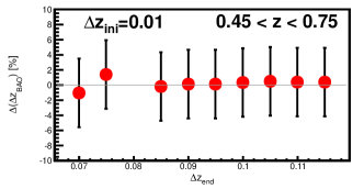
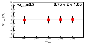
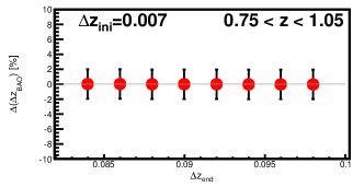
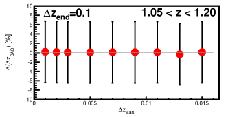
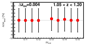
Figure 8: $\Delta z_{BAO}$ evolution as a function of the starting and end point of the fitted region. Results are stable, confirming that the systematic error is small. The error bars indicate the size of the statistical error, including Poisson shot noise and cosmic variance, for the used simulation, that covers 1/8 of the sky.

5.1.3 Galaxy Bias

At the BAO scales it is a good approximation to consider that the bias is scale independent (Cresswell & Percival, 2009; Crocce et al., 2011). It affects the radial correlation function not only as an overall normalization, but also through its effect in the redshift space distortions. Bias can influence the determination of the BAO scale only through the changes in the goodness of the parametrization of the correlation function for different biases. In order to estimate the contribution of the galaxy bias to the measurement of the radial BAO scale, we have repeated the analysis with different values of the bias, to obtain the propagation of the uncertainty in the galaxy bias for the selected galaxy population to the measured value of the radial BAO scale. The influence on the peak position is small, and we can estimate the associated systematic error as $\delta(\Delta z_{BAO})=0.15\%$.

Moreover, we have tested the effect of a scale dependent bias, introducing artificially the effect in the correlation functions, using an approximate Q-model with the determination of parameters from Cresswell & Percival (2009). The bias variation with $\Delta z$ in the fitted region of $\xi_{\parallel}(\Delta z)$ ranges from 1% to 6%, but the measurement of the BAO scale is insensitive to these changes. We estimate the systematic error in the presence of a scale dependent bias as $\delta(\Delta z_{BAO})=0.20\%$.

5.1.4 Starting and End Point of the Fit

To compute the systematic error associated to the parametrization method, we have done some further analysis on theoretical radial correlation functions with the same bin widths and central redshifts as those used in the analysis of the MICE simulation. The error associated to the method comes from the possible influence in the obtained $\Delta z_{BAO}$ of the range of $\Delta z$ used to perform the fit. To evaluate the error, we have varied this range for the 3 redshift bins where we have a significant detection of the BAO scale, and performed the fit for each range.

In the decision of the range to be fitted, we have to choose a starting point at angles smaller than the BAO peak, where the physics is determined by non-linearities, and an end point after the peak, beyond which the effects of cosmic variance may be relevant. By varying these two points we can study how much the result varies with this decision. Results can be seen in Fig. 8, where the obtained $\Delta z_{BAO}$ is shown for different starting points and end points of the fit, for the 3 redshift bins. In all cases, the uncertainty is of the order of 0.1%, which we assign as the associated systematic error. This uncertainty is much smaller than the statistical error, including Poisson shot noise and cosmic variance, which is depicted as error bars.

5.1.5 Total Systematic Error

The different sources of the systematic errors are completely independent, and therefore, we can compute the total systematic error by summing quadratically these contributions, resulting on a value of $\delta_{SYS}(\Delta z_{BAO})=0.33\%$.

There are some other potential systematic errors, the gravitational lensing magnification, which introduces a small correlation between redshift bins, or those mainly associated to the instrumental effects which could affect the used galaxy sample. However, these effects are expected to be very small and we have neglected them in this analysis.

5.2 Cosmological Constraints

The evolution of the measured radial BAO scale, including the systematic errors, with redshift is shown in Figure 5. The cosmological model of the simulation is the solid line. The recovered BAO scale is perfectly compatible with the true model, demonstrating that the method works.

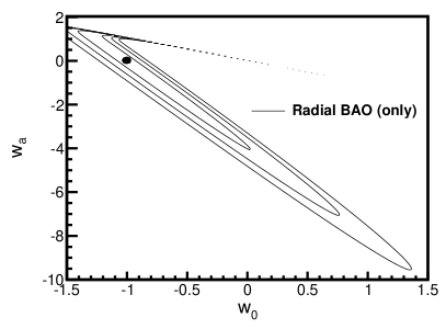
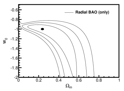
Figure 9: Contours at $1\sigma$, $2\sigma$ and $3\sigma$ C. L. on the plane $(w_{0},w_{a})$ (top) and on the plane $(\Omega_{M},w_{0})$ (bottom) obtained from the analysis of the radial BAO scale. The dot shows the value of the parameters for the MICE cosmology. No combination with any other cosmological probe is included. The other parameters have been fixed to the values of the MICE cosmology.

When these measurements are translated into constraints on the cosmological parameters, we obtain the results depicted in Figure 9, where the contours for $1\sigma$, $2\sigma$ and $3\sigma$ C. L. in the $(w_{0},w_{a})$ plane are shown at the top panel and the bottom panel shows the same contours in the $(\Omega_{M},w_{0})$ plane. To obtain the constraints on the cosmological parameters, we have performed a $\chi^{2}$ fit to the evolution of the measured radial BAO scale with the redshift to the model, where

$$\Delta z_{BAO}=r_{S}(\Omega_{M},w_{0},w_{a}...)~{}H(z,\Omega_{M},w_{0},w_{a}...),$$ (2)

where $r_{S}$ is the sound horizon scale at the baryon drag epoch and $H(z,\Omega_{M},w_{0},w_{a}...)$ is the Hubble parameter. We leave free those cosmological parameters which are shown in the figures, while all other parameters have been kept fixed to their values for the simulation. The cosmology of the simulation is recovered, and the plot shows the sensitivity of the radial BAO scale alone, since no other cosmological probe is included in these constraints.

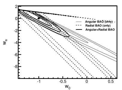
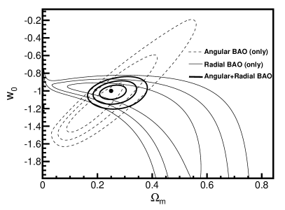
Figure 10: Contours at $1\sigma$, $2\sigma$ and $3\sigma$ C. L. on the plane $(w_{0},w_{a})$ (top) and on the plane $(\Omega_{M},w_{0})$ (bottom) from radial BAO (thin solid lines), angular BAO (thin dashed lines) and the combination of both (thick solid lines). The dot shows the value of the parameters for the MICE cosmology. No other cosmological probe is included in this result, showing the high sensitivity that the BAO standard ruler can achieve. The other parameters have been fixed to their values in the MICE cosmology.

5.3 Combination of Radial and Angular BAO Scales

We have applied the method of Sánchez et al. (2011) to determine the angular BAO scale for the same simulation. The results of this analysis are presented in the Appendix B. We have combined the results of this analysis with the radial BAO scale, using the same approach of the previous section. For the angular analysis, the BAO scale is described as

$$\theta_{BAO}=\frac{r_{S}(\Omega_{M},w_{0},w_{a}...)}{(1+z)~{}d_{A}(z,\Omega_{M},w_{0},w_{a}...)},$$ (3)

where $d_{A}(z,\Omega_{M},w_{0},w_{a}...)$ is the angular diameter distance. The constraints on the $(w_{0},w_{a})$ plane coming from this determination of the angular BAO scale can be seen in Figure 10 (top) as thin dashed lines, and correspond to the $1\sigma$, $2\sigma$ and $3\sigma$ C. L. contours. The sensitivity of the angular BAO scale is complementary to that of the radial BAO, shown as the thin solid lines. When combined, the contours represented by the thick solid lines are found. The same constraints for the $(\Omega_{M},w_{0})$ plane are shown in the bottom panel of Figure 10. These constraints are as precise as what is usually quoted for the BAO standard ruler, which is based on the use of the monopole of the 3-D correlation function. It is important to remark that these constraints are obtained ONLY with the BAO standard ruler, independently of any other cosmological probe, which shows the real power of the standard ruler method when the full information is used.

We provide also the combined result of BAO, both radial and angular, with the distance measurements from CMB using the WMAP7 covariance matrix (Komatsu et al., 2011) and assuming the measurements correspond to the MICE cosmology. The combination has been performed following the procedure as detailed in Komatsu et al. (2009). The corresponding contours at $1\sigma$, $2\sigma$ and $3\sigma$ C. L. are presented in Figure 11 both in the plane $(w_{0},w_{a})$ (top) and in the plane $(\Omega_{M},w_{0})$ (bottom) as thick solid lines, and compared with the result using only BAO (both radial and angular), which is presented as the thin lines. As before, the other parameters have been kept fixed. There is an important improvement in the precision of the determination of the corresponding parameters in both cases, larger in the $(\Omega_{M},w_{0})$ plane, showing that a precise measurement can be achieved when all the information provided by the BAO scale is included in the fit.

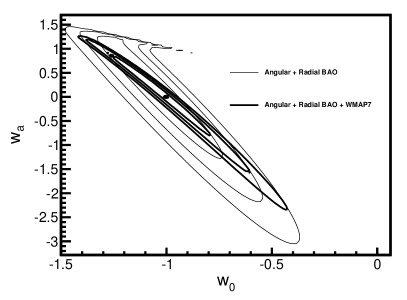
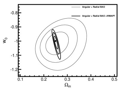
Figure 11: Contours at $1\sigma$, $2\sigma$ and $3\sigma$ C. L. on the plane $(w_{0},w_{a})$ (top) and on the plane $(\Omega_{M},w_{0})$ (bottom) from BAO (both radial and angular), depicted as thin solid lines, and adding also the CMB measurements, depicted as thick solid lines. The dot shows the value of the parameters for the MICE cosmology. The covariance matrix of WMAP7 has been used, while the central value of the measurement has been taken at the MICE cosmology. The other parameters have been fixed to their values in the MICE cosmology.

5.4 Comparison with Other Methods

In order to compare our results, obtained combining radial and angular BAO scale determinations, with the standard approach of measuring the position of the sound horizon scale in the monopole of the two-point correlation function, we performed on our mock catalogue the same analysis that was carried out to obtain the latest BAO detection by the BOSS collaboration (Anderson et al., 2012). For this we calculated the three-dimensional correlation function $\xi(r)$ using the Landy and Szalay estimator in the three wide redshift bins used for the analysis of the radial BAO ($0.45<z<0.75$, $0.75<z<1.10$ and $1.10<z$). We chose these wide bins in order to maximize the number of pairs that contribute to the measurement of the monopole, since this is one of the key advantages of the standard method. In order to calculate $\xi(r)$, redshifts must be translated into distances. We have used the true cosmology of the MICE simulation to ensure that our results will not be biased by this choice.

The covariance matrix for the monopole was calculated using the Gaussian approach described by Xu et al. (2013). This calculation was, again, validated by comparing it with the errors computed from subsamples of the total catalogue, and both estimations were found to be compatible within the range of scales needed for the analysis.

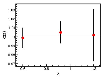
Figure 12: Values of the scaling parameter $\alpha$ measured from the three bins of the MICE mock catalogue. The input cosmology ($\alpha\equiv 1$) is recovered well within errors.

As is done in (Anderson et al., 2012), we fit the model

$$\xi_{\rm fit}(r)=B^{2}\,\xi_{\rm th}(\alpha\,r)+a_{0}+\frac{a_{1}}{r}+\frac{a_{2}}{r^{2}},$$ (4)

to the estimated correlation monopoles. Here $\xi_{\rm th}(r)$ is a template theoretical correlation function corresponding to the fiducial cosmological model used to translate redshifts into distances in the survey (in our case the MICE cosmology). This template was calculated from the CAMB linear power spectrum for the MICE cosmology, and corrected for non-linearities via the RPT damping factor. We are mainly interested in the fitting parameter $\alpha$, which relates real and fiducial scales:

$$\frac{d_{V}(z)}{r_{s}}=\alpha\,\frac{d_{V}^{\rm fid}(z)}{r_{s}^{\rm fid}},$$ (5)

where $d_{V}(z)\equiv((1+z)^{2}\,d_{A}^{2}(z)\,z/H(z))^{1/3}$ is the volume-averaged distance defined by Eisenstein et al. (2005). Since the true cosmology was used to translate redshifts into distances, the value of $\alpha$ must be compatible with 1 (within errors). The statistical uncertainty in $\alpha$ was calculated following the same method used in Anderson et al. (2012).

We have not studied the different sources of systematic errors for this measurement, and no systematic contribution has been added to the errors. On the one hand this provides a more conservative comparison with our approach, since the results quoted in section 5.3 do contain systematics. On the other hand, there exist several potential systematics that are specific for the standard method, such as the effect of the fiducial cosmology used to obtain the three-dimensional positions of the galaxies, or the choice of template used to perform the fit. Studying this effect would be extremely interesting, but we have postponed this analysis for a future work. As we have seen before, the systematic errors that are common to both approaches (bias, RSDs, non-linearities, fitting limits) are clearly subdominant compared to the statistical uncertainties.

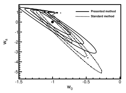
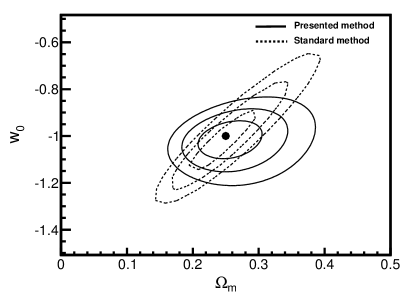
Figure 13: Contours at 1-$\sigma$, 2-$\sigma$ and 3-$\sigma$ confidence level in the planes $(w_{0},w_{a})$ (left panel) and $(\Omega_{\rm M},w_{0})$ (right panel). The solid contours correspond to our combination of independent radial and angular BAO information, while the dashed lines correspond to the results drawn from the standard analysis of the angle-averaged BAO. The different correlation between parameters is due to the different treatment of the redshift space distortions.

The cosmological constraints drawn in the $(\Omega_{\rm M},w_{0})$ and $(w_{0},w_{a})$ planes from the values of $\alpha$ measured from the correlation functions are shown in Figure 13. The figure also shows the contours corresponding to the combination of radial and angular information, described in the previous section, for comparison. Plots show that the constraining power of both methods is very similar. There is a degenerate direction in the $(\Omega_{\rm M},w_{0})$ plane for the standard method, which coincides with the orientation of the contours for the angular BAO shown in Figure 10 (bottom panel). This is a reasonable result: most of the information in the angle-averaged BAO signature comes from the angular part, since there are two transverse dimensions and only one longitudinal. On the other hand, our combined approach seems to be able to obtain better constraints on the evolution of the dark energy equation of state. This could be due to the fact that the radial BAO enables us to measure the evolution of the expansion rate alone, which is a local quantity, unlike the angular diameter distance, which is an integrated one depending on the expansion history. Although the degenerate directions are very similar for both methods, they are not exactly the same. The reason is the different treatment of the redshift space distortions, which are ignored, to first approximation, in the standard method when the angular average is performed. However, they are fully taken into account in our proposal, where the angular and radial correlation functions have very different shapes, mainly because of the redshift space distortions.

6 Conclusions

We have developed a new method to measure the BAO scale in the radial two-point correlation function. This method is adapted to the observational characteristics of galaxy surveys, where only the angular position on the sky and the redshift are measured for each galaxy. The sound horizon scale can be recovered from the non-linear radial correlation functions to a very high precision, only limited by the volume of the considered survey, since the systematic uncertainties associated to the determination of the BAO scale are very small, around 0.3%. On the other hand, the method is fully cosmology independent, since it relies only on observable quantities and, consequently, its results can be analyzed in any cosmological model.

The method has been tested with a mock catalogue built upon a large N-body simulation provided by the MICE collaboration, in the light cone and including redshift space distortions. The true cosmology is recovered within 1-$\sigma$. An evaluation of the main systematic errors has been included in this study, and we find that the method is very promising and very robust against systematic uncertainties. Note that this analysis over the MICE simulations is done on dark matter particles, instead of galaxies. We believe this simplification is not an essential limitation to the method presented here, as we have shown that both the modeling and the error analysis are quite generic.

We have compared the cosmological constraints obtained by combining radial and angular BAO information with those obtained by performing the standard analysis of the angle-averaged BAO signature on the same dataset and with the same fitting technique. Both methods seem to yield comparable constraints, with the advantage that our method is entirely based on purely observable quantities (redshifts and angles) and is therefore completely model-independent.

Appendix A Gaussian approach to estimate the covariance matrix of the 3-D correlation function

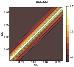
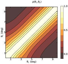
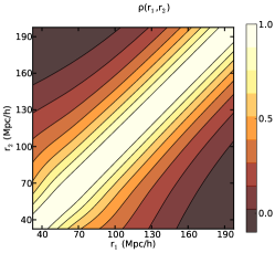
Figure 14: Reduced Gaussian covariance matrices for the radial (left), angular (center) and monopole correlation functions. The covariances in the first and last cases were computed for a survey with 5000 square-degrees in $0.45<z<0.75$, while the angular case was computed for a bin $0.5<z<0.6$. In the three cases the axis ranges correspond to similar comoving scales.

We have used a theoretical estimation of the covariance matrix for the 3-D correlation function, which is then applied to the estimation of the covariance for the radial correlation function. Our approach is based on assuming Gaussian statistics for the overdensity field, in analogy with the approach in Xu et al. (2013) for the monopole and with the method described in Crocce et al. (2011) for the angular correlation function. We have used the following convention for the power spectrum:

$$\langle\delta_{\bm{k}}\delta_{{\bm{k}}^{\prime}}\rangle =\delta^{D}(\bm{k}+\bm{k}^{\prime})\left(P({\bf k})+\bar{n}^{-1}\right)$$ (6)

$$=\frac{V}{(2\pi)^{3}}\delta^{K}_{\bm{k}-\bm{k}^{\prime}}\left(P({\bf k})+\bar{n}^{-1}\right)$$ (7)

where $\delta^{D}$ and $\delta^{K}$ are the Dirac and Kronecker deltas, $V$ is the volume and we have taken into account the Poisson contribution to the total variance as the inverse of the number density of sources $\bar{n}$.

The anisotropic power spectrum can be estimated from a given realization of $\delta_{\bf k}$ by averaging over the symmetric azimuthal angle:

$$\hat{P}(k_{\parallel},k_{\perp})\equiv\frac{1}{2\pi}\int_{0}^{2\pi}d\phi_{k}\left(\frac{(2\pi)^{3}}{V}|\delta_{\bf k}|^{2}-\frac{1}{\bar{n}}\right)$$ (8)

Assuming that $\delta_{\bm{k}}$ is Gaussianly distributed we can obtain the covariance for this estimator using Wick’s theorem:

$$C^{P}({\bf k}_{1},{\bf k}_{2})= \frac{4\pi^{2}}{V}\mathfrak{P}^{2}(k_{\parallel},k_{\perp})\frac{\delta^{\mathcal{D}}(k_{2,\perp}-k_{1,\perp})}{k_{1,\perp}}$$

$$\left[\delta^{\mathcal{D}}(k_{2,\parallel}-k_{1,\parallel})+\delta^{\mathcal{D}}(k_{2,\parallel}+k_{1,\parallel})\right],$$ (9)

where, as is done in Xu et al. (2013), the effect of a non-homogeneous number density $\bar{n}(z)$ has been taken into account by defining the volume-averaged variance

$$\mathfrak{P}^{-2}(k_{\parallel},k_{\perp})\equiv\int\frac{dV(z)}{P(k_{\parallel},k_{\perp})+\bar{n}^{-1}(z)}.$$

The anisotropic power spectrum can be related to the anisotropic correlation function using the 0-order cylindrical Bessel function $J_{0}(x)$ through

$$\xi(\pi,\sigma)=\frac{1}{4\pi^{2}}\int_{-\infty}^{\infty}dk_{\parallel}e^{i\,k_{\parallel}\pi}\int_{0}^{\infty}dk_{\perp}k_{\perp}J_{0}(k_{\perp}\sigma)P(k_{\parallel},k_{\perp}),$$

And thus the covariance matrix for $\xi$ can be calculated as

$$C^{\xi}({\bf r}_{1},{\bf r}_{2})\equiv \frac{1}{\pi^{2}}\int_{0}^{\infty}dk_{\parallel}\,\bar{\cos}(k_{\parallel}\pi_{1})\,\bar{\cos}(k_{\parallel}\pi_{2})$$

$$\int_{0}^{\infty}dk_{\perp}k_{\perp}\bar{J}_{0}(k_{\perp}\sigma_{1})\,\bar{J}_{0}(k_{\perp}\sigma_{2})\mathfrak{P}^{2}(k_{\parallel},k_{\perp}).$$ (10)

Here we have taken into account the finiteness of the bins $\Delta\pi$, $\Delta\sigma$ by defining the regularized functions $\bar{\cos}$ and $\bar{J}_{0}$:

$$\bar{\cos}(k_{\parallel}\pi)\equiv\frac{\sin(x_{2})-\sin(x_{1})}{x_{2}-x_{1}},\hskip 6.0pt(x_{1,2}\equiv k_{\parallel}(\pi\pm\Delta\pi))$$

$$\bar{J}_{0}(k_{\perp}\sigma)\equiv 2\,\frac{x_{2}\,J_{1}(x_{2})-x_{1}\,J_{1}(x_{1})}{x_{2}^{2}-x_{1}^{2}},\hskip 6.0pt(x_{1,2}\equiv k_{\perp}(\sigma\pm\Delta\sigma))$$

From this result it is straightforward to compute the covariance matrix for the radial correlation function ($\sigma_{1,2}=0$) as

$$C^{\xi}_{\parallel}(\pi_{1},\pi_{2})\equiv\frac{1}{\pi^{2}}\int_{0}^{\infty}dk_{\parallel}\,\bar{\cos}(k_{\parallel}\pi_{1})\,\bar{\cos}(k_{\parallel}\pi_{2})\,\left[\mathfrak{P}_{\parallel}(k_{\parallel},\Delta\sigma)\right]^{2},$$ (11)

where we have defined the projected $k$-space variance

$$\left[\mathfrak{P}_{\parallel}(k_{\parallel},\Delta\sigma)\right]^{2}\equiv\int^{\infty}_{0}dk_{\perp}\,k_{\perp}\left[2\frac{J_{1}(k_{\perp}\,\Delta\sigma)}{k_{\perp}\,\Delta\sigma}\right]^{2}\mathfrak{P}^{2}(k_{\parallel},k_{\perp}).$$ (12)

Here the radial coordinate $\pi$ is related to the redshift separation through $\Delta z\equiv\pi\,H(z)$, and the transverse width $\Delta\sigma$ is related to the angular pixel resolution through $\Delta\theta\equiv\Delta\sigma/r(z)$. As can be verified on closer inspection of equation 12, the covariance grows dramatically as we decrease the pixel size. This is due to the fact that the number of galaxy pairs drops and the errors become shot-noise dominated.

Throughout this work, Gaussian estimations for the covariance matrices were used. Figure 14 shows the Gaussian predictions for the reduced covariance matrix $\rho_{ij}\equiv C_{ij}/\sqrt{C_{ii}\,C_{jj}}$ of the radial correlation function (left panel), the angular correlation function (central panel) and the monopole (right panel). The axis ranges correspond to similar comoving scales in the three cases. Notice that, while the errors on the radial correlation function are almost diagonal, they are correlated over a large range of scales in the angular (transverse) case. For the monopole, the errors are also correlated over a large number of bins, which is a sensible result, since the monopole corresponds to an angular average over two transverse and one longitudinal directions.

Appendix B Angular BAO results for the Combination

The angular BAO measurements we have used for the results presented in the text have been obtained applying the method described in Sánchez et al. (2011) to the cosmological simulation used in this paper. We have used 10 redshift bins of width 0.1, starting at redshift 0.2 up to redshift 1.2. We find statistically significant results in 9 of them. Results are presented in Figure 15. These are the results we combine with the radial BAO in order to obtain the cosmological constraints presented in the text. It is important to notice that the redshifts for this galaxy sample are spectroscopic and consequently, the systematic error associated to the photometric redshift that is quoted on Sánchez et al. (2011) does not affect these measurements.

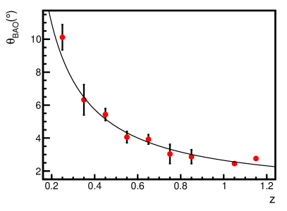
Figure 15: Measured angular BAO scale as a function of the redshift in the MICE simulation using the method described in Sánchez et al. (2011). Dots are the measured values of $\theta_{BAO}$ and the solid line is the prediction for the cosmology of the simulation.

References

- Abdalla et al. (2012) Abdalla F., et al., 2012, arXiv:1209.2451 [astro-ph]
- Anderson et al. (2012) Anderson L., et al., 2012, MNRAS, 427, 3435
- Bonvin & Durrer (2011) Bonvin C., Durrer R., 2011, PRD, 84, 063505
- Carnero et al. (2012) Carnero A., Sánchez E., Crocce M., Cabré A., Gaztañaga E., 2012, MNRAS, 419, 1689
- Cresswell & Percival (2009) Cresswell J. G., Percival W. J., 2009, MNRAS, 392, 682
- Crocce et al. (2011) Crocce M., Cabré A., Gaztañaga E., 2011, MNRAS, 414, 329
- Crocce et al. (2010) Crocce M., Fosalba P., Castander F. J., Gaztañaga E., 2010, MNRAS, 403, 1353
- Crocce & Scoccimarro (2006) Crocce M., Scoccimarro R., 2006, PRD, 73, 063519
- Eisenstein et al. (2005) Eisenstein D. J., et al., 2005, ApJ, 633, 560
- Fosalba et al. (2008) Fosalba P., Gaztañaga E., Castander F. J., Manera M., 2008, MNRAS, 391, 435
- Gaztañaga et al. (2009) Gaztañaga E., Cabré A., Hui L., 2009, MNRAS, 399, 1663
- Hütsi (2006a) Hütsi G., 2006a, A&A, 449, 891
- Hütsi (2006b) Hütsi G., 2006b, A&A, 459, 375
- Kaiser (1987) Kaiser N., 1987, MNRAS, 227, 1
- Kazin et al. (2010) Kazin E. A., Blanton M. R., Scoccimarro R., McBride C. K., Berlind A. A., Bahcall N. A., Brinkmann J., Czarapata P., Frieman J. A., Kent S. M., Schneider D. P., Szalay A. S., 2010, ApJ, 710, 1444
- Komatsu et al. (2009) Komatsu E., et al., 2009, ApJS, 180, 330
- Komatsu et al. (2011) Komatsu E., et al., 2011, ApJS, 192, 18
- Landy & Szalay (1993) Landy S. D., Szalay A. S., 1993, ApJ, 412, 64
- Laureijs et al. (2011) Laureijs R., et al., 2011, arXiv:1110.3193 [astro-ph]
- Lewis et al. (2000) Lewis A., Challinor A., Lasenby A., 2000, ApJ, 538, 473
- Okumura et al. (2008) Okumura T., Matsubara T., Eisenstein D. J., Kayo I., Hikage C., Szalay A. S., Schneider D. P., 2008, ApJ, 676, 889
- Padmanabhan et al. (2007) Padmanabhan N., et al., 2007, MNRAS, 378, 852
- Peebles (1980) Peebles P. J. E., ed. 1980, The Large-Scale Structure of the Universe. Princeton University Press
- Percival et al. (2007) Percival W. J., Cole S., Eisenstein D. J., Nichol R. C., Peacock J. A., Pope A. C., Szalay A. S., 2007, MNRAS, 381, 1053
- Sánchez et al. (2009) Sánchez A. G., Crocce M., Cabré A., Baugh C. M., Gaztañaga E., 2009, MNRAS, 400, 1643
- Sánchez et al. (2011) Sánchez E., Carnero A., García-Bellido J., Gaztañaga E., de Simoni F., Crocce M., Cabré A., Fosalba P., Alonso D., 2011, MNRAS, 411, 277
- Schlegel et al. (2011) Schlegel D., et al., 2011, arXiv: 1106.1706 [astro-ph]
- Xu et al. (2013) Xu X., Cuesta A. J., Padmanabhan N., Eisenstein D. J., McBride C. K., 2013, MNRAS, 431, 2834