Motion Control of a Spinning Disc on Rotating Earth

Abstract

This paper considers the motion control of a particle and a spinning disc on rotating earth. The equations of motion are derived using Lagrangian mechanics. Trajectory planning is studied as an optimization problem using the method referred to as Discrete Mechanics and Optimal Control.

1 Introduction

This paper considers the motion control of a particle and a spinning disc on earth. In particular, we derive the governing equations using Lagrangian mechanics and study trajectory planning as an optimization problem using the method referred to as Discrete Mechanics and Optimal Control, see [4, 5].

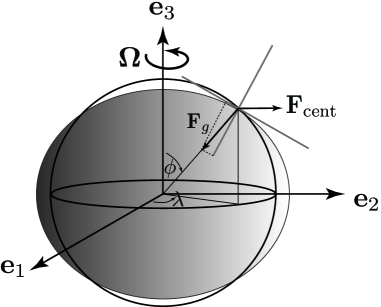
Figure 1: The earth (oblate spheroid) is modeled as a rotating sphere with an added potential used to emulate the effect of the eccentricity which produces a non-zero horizontal component of gravity.

1.1 Problem Description

Consider the horizontal motion on earth in the absence of friction and pressure gradient forces. A perfect sphere model fails to capture the dynamical effects associated with the horizontal component of gravity due to the eccentricity of the earth, as shown in Figure 1 and discussed in [1, 10, 11, 12, 13] for a particle moving on rotating earth. It also plays an important role in the unsteady dynamics of a spinning disc on rotating earth as investigated in [6, 14, 15] as a model for geophysical vortex motion. In both problems, the authors emulated the effect of the earth eccentricity by adding an artificial potential to the perfect sphere model. In this paper, we use the same model to address the problem of planning the motion on earth as an optimization problem based on a Lagrangian formulation. More specifically, we investigate optimal trajectories that steer the particle or the spinning disc from an initial position and velocity to a final position and velocity while minimizing a prescribed cost function such as the control effort.

1.2 Motivation

The main motivation for these problems comes from atmospheric sciences where one needs to track atmospheric drifters over periods of days, weeks, or even months. In the simplest case, these drifters are high altitude balloons which, to a first order approximation, can be thought of as passive tracers. However, if complex dynamical maneuvers are required, it is useful to include more complicated internal dynamics, such as rotational motion, which adds interesting new effects. These kinds of finite-dimensional models have also been used as mechanical models of vortex motion in some geophysical settings [6] and one could imagine thinking of the spinning disc model, in the limit as the ratio of the disc radius to the radius of the sphere goes to zero, as a “point-vortex”, a collection of which might approximate a distribution of vorticity [8]. Interestingly, systems of interacting rotating millimeter-sized discs floating on a liquid-air interface have been used recently [3] to study self-assembly of patterns in models that have some of the same pattern forming features as a wide range of vortex lattice systems. We consider the optimal control problems treated in this paper as a first step in the process of attempting to implement control and motion strategies in these contexts.

1.3 Organization of the Paper

In Section 2, we formulate the dynamics of a particle and a spinning disc moving on earth, and address the question of motion planning in Section 3. The numerical implementation and discussion of the results are presented in Section 4.

2 Dynamics on Rotating Earth

Consider a particle of mass $m$ moving on a sphere of radius $R$ and subject only to a gravitational force pointing towards the center of the sphere and a supporting force normal to the surface of the sphere (i.e., pointing in the opposite direction of gravity). One distinguishes two types of behavior relative to a fixed inertial frame $\{\mathbf{E}_{i}\}_{i=1,2,3}$ as follows: if the initial velocity is zero, the particle remains at rest for all time, otherwise, it moves along a great circle which passes through the starting position and is tangent to the direction of the initial velocity at the starting point. If the sphere is rotating, say with an angular velocity vector $\bm{\Omega}=\Omega\,\mathbf{E}_{3}$ where $\Omega=2\pi/1$day, the motion of the particle can be described relative to either a fixed inertial frame or a frame rotating with the sphere $\{\mathbf{e}_{i}\}_{i=1,2,3}$ with $\mathbf{e}_{3}=\mathbf{E}_{3}.$ In the inertial frame, one sees the same types of trajectories as in the stationary sphere case. The motion appears more complicated in the rotating frame where Coriolis and centrifugal forces need to be taken into consideration. An important observation here is that a particle starting at rest relative to the moving frame does not remain at rest due to the horizontal component of the centrifugal force, i.e., the component in the direction tangent to the earth surface. However, a particle starting at rest relative to the rotating earth remains at rest for all time. Indeed, in a more accurate model of the earth where the effect of eccentricity is taken into account, the horizontal component of the centrifugal force $\mathbf{F}_{\rm cent}$ is counterbalanced by the horizontal component of the gravitational force $\mathbf{F}_{g}$. Recall that $\mathbf{F}_{\rm cent}$ is given by:

$$\mathbf{F}_{\rm cent}=-m\,\bm{\Omega}\times(\bm{\Omega}\times\mathbf{R}),$$ (1)

where $\mathbf{R}$ denotes the position vector of the particle on the sphere. It is convenient to introduce spherical coordinates $(\phi,\lambda)$ measured relative to the moving frame $\{\mathbf{e}_{i}\}$, see Figure 1, and an associated right-handed orthonormal basis $\{\mathbf{e}_{\phi},\mathbf{e}_{\lambda},\mathbf{e}_{R}\}.$ The centrifugal force $\mathbf{F}_{\rm cent}$ can then be expressed as follows:

$$\mathbf{F}_{\rm cent}=mR\,\Omega^{2}\sin\phi\,(\sin\phi\,\mathbf{e}_{R}+\cos\phi\,\mathbf{e}_{\phi}).$$ (2)

To cancel the horizontal component of $\mathbf{F}_{\rm cent}$, the particle should be subject to a horizontal force opposite in direction and of magnitude equal to $mR\Omega^{2}\sin\phi\cos\phi$. One way to incorporate this effect yet retain the obvious advantages of spherical coordinates with constant radius is to introduce a potential function $V_{a}$ whose gradient in the horizontal direction produces such force, [13], namely,

$$V_{a}=\frac{1}{2}\,mR^{2}\,\Omega^{2}\,\sin^{2}\phi.$$ (3)

2.1 Equations of Motion for a Particle

The Lagrangian function for the system is given by:

$$L(q,\dot{q})=T-V,$$ (4)

where $T$ and $V$ denote the kinetic and potential energies, respectively, while $q$ parameterizes the position of the particle on earth and can be chosen as $q=(\phi,\lambda)$. Lagrange’s equations of motion are given by Hamilton’s principle (also known as the least action principle). This principle amounts to taking variations of the action, between a fixed initial time $t_{0}$ and a fixed final time $t_{f}$,

$$S=\int_{t_{0}}^{t_{f}}L\,{\rm d}t$$ (5)

with respect to arbitrary variations $\delta q$ of the path that keep the endpoints $q(t_{0})$ and $q(t_{f})$ fixed. The point-wise equations of motion thus obtained are of the form:

$$\dfrac{{\rm d}}{{\rm d}t}\dfrac{\partial L}{\partial\dot{q}}-\dfrac{\partial L}{\partial{q}}=0.$$ (6)

The kinetic energy $T$ of the particle can be expressed in terms of spherical coordinates as:

$$T=\frac{1}{2}\,mR^{2}\left[{\dot{\phi}}^{2}+(\dot{\lambda}+\Omega)^{2}\sin^{2}\phi\right].$$ (7)

The potential energy is the sum of two parts, the gravitational potential $V_{g}$ which is a constant and therefore can be set to zero, and the artificial potential $V_{a}$ introduced in (3). Lagrange’s equations (6) read as:

$$\begin{cases}\ddot{\phi}-\dot{\lambda}\Omega\sin 2\phi-\dfrac{1}{2}\,{\dot{\lambda}}^{2}\sin 2\phi=0,\\[4.30554pt] \ddot{\lambda}+2\,\dot{\phi}\,(\dot{\lambda}+\Omega)\cot\phi=0.\end{cases}$$ (8)

Finally, note that, since $L$ is not an explicit function of longitude $\lambda$ and time $t$, by Noether’s theorem, one has two integrals of motion (conserved quantities) associated with these symmetries. The angular momentum in the $\mathbf{e}_{\lambda}$-direction is conserved,

$$\pi_{\lambda}=mR^{2}(\dot{\lambda}+\Omega)\sin^{2}\phi={\rm constant},$$

and the total energy $E$ is conserved

$$E=\frac{1}{2}mR^{2}\left[{\dot{\phi}}^{2}+(\dot{\lambda}+\Omega)^{2}\sin^{2}\phi\right]+\frac{1}{2}mR^{2}\Omega^{2}\sin^{2}\phi={\rm constant}.$$

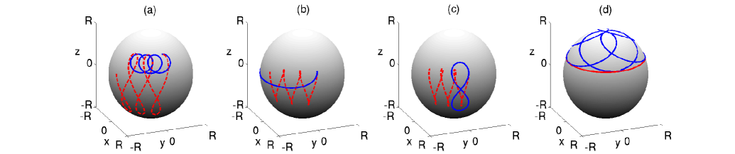
Figure 2: Free motion of a particle of mass $m$ on a rotating earth and rotating sphere, the solid line is the trajectory on earth, dashed line is on sphere. End time is 3 days for all examples, initial conditions are: (a) $(\phi_{0},\lambda_{0})=(\pi/4,0)$, $(\dot{\phi}_{0},\dot{\lambda}_{0})=(0,2)$; (b) $(\phi_{0},\lambda_{0})=(3\pi/8,0)$, $(\dot{\phi}_{0},\dot{\lambda}_{0})=(0.92,0)$; (c) $(\phi_{0},\lambda_{0})=(3\pi/8,0)$, $(\dot{\phi}_{0},\dot{\lambda}_{0})=(1.366,0)$; (d) $(\phi_{0},\lambda_{0})=(3\pi/8,0)$, $(\dot{\phi}_{0},\dot{\lambda}_{0})=(0,-2\pi)$.

2.2 Equations of Motion for a Spinning Disc

Consider a thin disc, of radius $a$ and uniformly distributed mass $m$, tangent to the earth surface such that its center of mass lies on earth and can be parameterized by $(\phi,\lambda)$. The disc is free to rotate or spin about its axis of symmetry which, by assumption, remains normal to the earth surface at all time. That is, the disc is free to spin about the $\mathbf{e}_{R}$-axis.

The Lagrangian function of the spinning disc is given by (4). The kinetic energy can be decomposed into a translation kinetic energy which has the same form as in (7) and a rotational kinetic energy $T_{\rm rot}$, which can be expressed as:

$$T_{\rm rot}=\frac{1}{2}I_{h}\,\omega_{\phi}^{2}+\frac{1}{2}I_{h}\,\omega_{\lambda}^{2}+\frac{1}{2}I_{v}\,\omega_{\psi}^{2},$$ (9)

where $I_{v}=\frac{1}{2}ma^{2}$ and $I_{h}=\frac{1}{4}ma^{2}$ are the moments of inertia of the disc about $\mathbf{e}_{R}$ and about the horizontal axes $\mathbf{e}_{\phi}$ and $\mathbf{e}_{\lambda}$, respectively. In (9), the components of the angular velocity relative to the spherical basis $\{\mathbf{e}_{\phi},\mathbf{e}_{\lambda},\mathbf{e}_{R}\}$ are given by:

$$\omega_{\phi}=\dot{\phi},\quad\omega_{\lambda}=(\dot{\lambda}+\Omega)\sin\phi,\quad\omega_{\psi}=\dot{\psi}+(\dot{\lambda}+\Omega)\cos\phi.$$ (10)

Now, use $M=mR^{2}$, substitute (10) in (9) and add (7) to get the total kinetic energy

$$T=\frac{1}{2}\,(M+I_{h})\left[{\dot{\phi}}^{2}+(\dot{\lambda}+\Omega)^{2}\sin^{2}\phi\right]+\frac{1}{2}\,I_{v}\left[\dot{\psi}+(\dot{\lambda}+\Omega)\cos\phi\right]^{2}.$$ (11)

To simplify the expression for the potential energy, we assume that $a\ll R$ and treat the gravitational and artificial potentials, $V_{g}$ and $V_{a}$, as functions of the center of mass only. In addition to $V_{g}$ and $V_{a}$, the disc is subject to a potential function $V_{d}$ of the form

$$V_{d}=\frac{1}{2}\,I_{v}\,\Omega^{2}\cos^{2}\phi,$$ (12)

which, as $V_{a}$, is due to the fact that the dynamics is described in a rotating frame. To better understand the potential $V_{d}$, consider the special case when the disc is stationary in inertial frame and its center of mass is placed at the north pole $\phi=0$. Clearly, relative to the rotating frame, the disc is not stationary and has total energy $\frac{1}{2}I_{v}\Omega^{2}$, which is exactly $V_{d}|_{\phi=0}$. The total potential energy $V=V_{g}+V_{a}+V_{d}$ can then be expressed as

$$V\ =\ \frac{1}{2}\,\Omega^{2}(M\sin^{2}\phi+I_{v}\cos^{2}\phi),$$ (13)

where, as before, $V_{g}$ is constant and is set equal to zero. Lagrange’s equations (6) for the spinning disc, with $q=(\phi,\lambda,\psi)$ and $I_{v}=2I_{h}=2I$, yield

$$\begin{cases}(M+I)\ddot{\phi}=-2I\dot{\psi}(\dot{\lambda}+\Omega)\sin\phi+\dfrac{1}{2}\left[(M-I)(\dot{\lambda}+\Omega)^{2}-(M-2I)\Omega^{2}\right]\sin 2\phi,\\[4.30554pt] (M+I)\ddot{\lambda}\sin\phi=2I\dot{\psi}\dot{\phi}-2M(\dot{\lambda}+\Omega)\dot{\phi}\cos\phi,\\[4.30554pt] (M+I)\ddot{\psi}\sin\phi=-2I\dot{\psi}\dot{\phi}\cos\phi+\left[M(1+\cos^{2}\phi)+I\sin^{2}\phi\right](\dot{\lambda}+\Omega)\dot{\phi}.\end{cases}$$ (14)

The Lagrangian function $L$ does not depend explicitly on $\lambda$, $\psi$ and time $t$ which implies the existence of three integrals of motion. The angular momenta $\pi_{\lambda}$ and $\pi_{\psi}$ in the $\mathbf{e}_{\lambda}$ and $\mathbf{e}_{R}$ directions are conserved,

$$\begin{cases}\pi_{\lambda}=(M+I)(\dot{\lambda}+\Omega)\sin^{2}\phi+2I\left[\dot{\psi}\cos\phi+(\dot{\lambda}+\Omega)\cos^{2}\phi\right]={\rm constant},\\[4.30554pt] \pi_{\psi}=I_{v}\left[\dot{\psi}+(\dot{\lambda}+\Omega)\cos\phi\right]={\rm constant},\end{cases}$$

as well as the total energy

$$E=\frac{1}{2}M\Omega^{2}\sin^{2}\phi+\frac{1}{2}(M+I)\left[{\dot{\phi}}^{2}+(\dot{\lambda}+\Omega)^{2}\sin^{2}\phi\right]+I\left\{\left[\dot{\psi}+(\dot{\lambda}+\Omega)\cos\phi\right]^{2}+\Omega^{2}\cos^{2}\phi\right\}={\rm constant}.$$

An approximate solution to (14) can be sought under the assumption that the disc translational velocity is much smaller than the velocity of the earth, i.e. $\dot{\phi}\ll\Omega$ and $\dot{\lambda}\ll\Omega$. The approximate solution, referred to as “steady drift” in [6], is:

$$\phi\approx\phi_{0},\quad\dot{\psi}\approx\dot{\psi}_{0},\quad\dot{\lambda}\approx\frac{1}{2}\frac{I_{v}}{M}\frac{\dot{\psi}_{0}}{\cos\phi_{0}}.$$ (15)

The comparison between this approximate solution and our direct numerical integration of (14) suggests that this is a good approximation under additional conditions (see Section 4 for more details). Namely, $\dot{\psi}$ has to be much larger than $\Omega$, say of the order $O(10\Omega)$. Also, it should be clear that the latitude $\phi$ must not be chosen close to the equator where $\dot{\lambda}$ obtained above is not accurate and the motions in $\phi$ and $\psi$ are too significant to ignore.

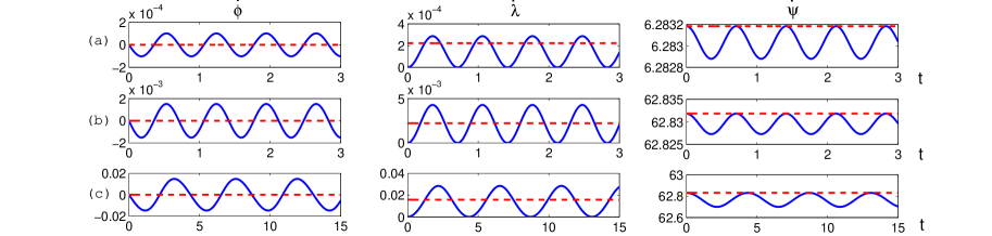
Figure 3: Free motion of a spinning disc on rotating earth, the solid line is the result of direct numerical integration, dashed line is an approximate solution. We present $\dot{\phi}$, $\dot{\lambda}$ and $\dot{\psi}$ in three columns respectively. Initial conditions and end times are: (a) $(\phi_{0},\lambda_{0})=(\pi/4,0)$, $(\dot{\phi}_{0},\dot{\lambda}_{0},\dot{\psi}_{0})=(0,0,\Omega)$, end time 3 days; (b) $(\phi_{0},\lambda_{0})=(\pi/4,0)$, $(\dot{\phi}_{0},\dot{\lambda}_{0},\dot{\psi}_{0})=(0,0,10\Omega)$, end time 3 days; (c) $(\phi_{0},\lambda_{0})=(\pi/2-0.1,0)$, $(\dot{\phi}_{0},\dot{\lambda}_{0},\dot{\psi}_{0})=(0,0,10\Omega)$, end time 15 days.

3 Motion Planning

The main point of this article is to investigate the problem of motion planning for the particle and the spinning disc moving on earth. In the case of the particle, we introduce control forces in both $\mathbf{e}_{\phi}$ and $\mathbf{e}_{\lambda}$ direction and solve for optimal control forces that steer the particle from an initial position and velocity to a desired final position and velocity. For the spinning disc, we apply a control torque about the axis of symmetry of the disc, i.e., a torque that controls the spin $\psi$ of the disc. Clearly, this spinning disc is under-actuated and questions of solvability and controllability are important.

3.1 Solvability and Controllability

The problem for the spinning disc is to find optimal torques that steer $\bigl{(}\phi(t_{0}),\lambda(t_{0}),\lambda(t_{0})\bigr{)}$ to $\bigl{(}\phi(t_{f}),\lambda(t_{f}),\lambda(t_{f})\bigr{)}.$ For some given initial and final conditions, there may be no control torque that achieves the desired motion. In this case the optimization problem has no solution.

In Section 4, we provide numerical evidence that the spinning disc can achieve a net motion on the earth surface under control mechanism. This suggests that the problem may be controllable or, at least, controllable in some finite regions of the earth surface. For a rigorous proof of controllability, one needs to appeal to controllability theorems for systems with drift, see, e.g., [9]. Such undertaken, although very important, is beyond the scope of the present paper.

3.2 Motion Control as an Optimization Problem

Take $q$ to be the state variables and let $f$ be the control force. For the case of a particle, one has $q=(\phi,\lambda)$ and $f=(f_{\phi},f_{\lambda})$ while for the spinning disc $q=(\phi,\lambda,\psi)$ and $f=(0,0,f_{\psi})$. The motion planning problem can then be stated as follows. Given the boundary conditions $q(t_{0})=q_{0}$, $\dot{q}(t_{0})=\dot{q}_{0}$ and $q(t_{f})=q_{f}$, $\dot{q}(t_{f})=\dot{q}_{f}$, find $f$ that minimizes the cost function

$$\int_{t_{0}}^{t_{f}}C(q,\dot{q},f)\,\rm{d}t$$ (16)

subject to the Lagrange-D’Alembert principle

$$\delta\int_{t_{0}}^{t_{f}}L(q,\dot{q})\,{\rm d}t\,+\int_{t_{0}}^{t_{f}}f\cdot\delta q\,{\rm d}t\,+\,p_{0}\cdot\delta q_{0}\,-\,p_{f}\cdot\delta q_{f}=0,$$ (17)

for all arbitrary variations $\delta q$. That is, the least action principle outlined in Section 2 is restated here as the Lagrange-d’Alembert principle (to account for external control forces) and without the a priori assumption that the variations vanish at the end points $t_{0}$ and $t_{f}$. Rather, this condition is imposed using the boundary constraints

$$\delta{q}_{0}=q(t_{0})-q_{0}=0\ ,\quad\delta q_{f}=q(t_{f})-q_{f}=0,$$ (18)

and their associated Lagrange multipliers

$$\left.p_{0}=\frac{\partial L}{\partial\dot{q}}\right|_{t_{0}},\quad\left.p_{f}=\frac{\partial L}{\partial\dot{q}}\right|_{t_{f}}.$$ (19)

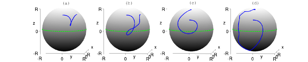
Figure 4: Optimal control results of particle on rotating earth, the solid line is trajectory under control, and dashed line is equator. Initial and final conditions for case (a) and (b) are: $(\phi_{0},\lambda_{0})=(\pi/4,0)$, $(\dot{\phi}_{0},\dot{\lambda}_{0})=(0,0)$, $(\phi_{f},\lambda_{f})=(\pi/4,\pi/3)$, $(\dot{\phi}_{f},\dot{\lambda}_{f})=(0,0)$, and the end times: (a) $t_{f}=$1 day, (b) $t_{f}$=3 days. Initial and final conditions for case (c) and (d) are: $(\phi_{0},\lambda_{0})=(\pi/3,0)$, $(\dot{\phi}_{0},\dot{\lambda}_{0})=(0,0)$, $(\phi_{f},\lambda_{f})=(\pi/8,0)$, $(\dot{\phi}_{f},\dot{\lambda}_{f})=(0,0)$, and the end times: (c) $t_{f}=$1 day, (d) $t_{f}$=3 days.

3.3 Discretization

We discretize the optimal control problem using the novel method devised by [4] where the idea is to discretize the cost function (16) and the variational principle (17) directly using global discretization of the states and the controls. To this end, a path $q(t)$, where $t\in[t_{0},t_{f}]$, is replaced by a discrete path $q_{d}:\{0,h,2h,\ldots,Nh=t_{f}]$, $N\in\mathbb{N}$. Here, $q_{d}(nh):=q_{n}$ is viewed as an approximation to $q(t_{n}=nh)$, $n\in\mathbb{N}$ and $n\leq N$. Similarly, the continuous force $f$ is approximated by a discrete force $f_{d}$ such that $f_{n}=f_{d}(nh)$.

The cost function (16) is approximated on each time interval $[nh,(n+1)h]$ by

$$C_{d}(q_{n},q_{n+1},f_{n},f_{n+1})\approx\int_{nh}^{(n+1)h}C(q,\dot{q},f)\,{\rm d}t,$$ (20)

which yields the discrete cost function

$$J_{d}(q_{d},f_{d})=\sum_{n=0}^{N-1}C_{d}(q_{n},q_{n+1},f_{n},f_{n+1}).$$ (21)

The action integral (17) is approximated on each time interval $[nh,(n+1)h]$ by a discrete Lagrangian

$$L_{d}(q_{n},q_{n+1})\approx\int_{nh}^{(n+1)h}L(q,\dot{q})\,{\rm d}t.$$ (22)

We also approximate $\int_{t_{n}}^{t_{n+1}}f\cdot\delta q\approx f_{n}^{-}\cdot\delta q_{n}+f_{n}^{+}\cdot\delta f_{n+1}$, where $f^{-}_{n}$ and $f^{+}_{n}$ are called left and right discrete torques, respectively. The discrete version of (17) requires one to find paths $\{q_{n}\}_{n=0}^{N}$ such that for all variations $\{\delta q_{n}\}_{n=0}^{N}$, one has

$$\delta\sum_{n=0}^{N-1}L_{d}(q_{n},q_{n+1})+\sum_{n=0}^{N-1}(f_{n}^{-}\cdot\delta q_{n}+f_{n}^{+}\cdot\delta q_{n+1})+p_{0}\cdot\delta q_{0}-p_{f}\cdot\delta q_{f}=0.$$ (23)

The discrete variational principle (23) yields the following equality constraints

$$\begin{cases}D_{2}L_{d}(q_{n-1},q_{n})+D_{1}L_{d}(q_{n},q_{n+1})+f_{n-1}^{+}+f_{n}^{-}=0,\\[4.30554pt] p_{0}+D_{1}L_{d}(q_{0},q_{1})+f_{0}^{-}=0,\\[4.30554pt] -p_{f}+D_{2}L_{d}(q_{N-1},q_{N})+f_{N}^{+}=0.\end{cases}$$ (24)

4 Implementation and Numerical Results

We now present some numerical results for free motion and motion planning of a particle and a spinning disc on earth.

4.1 Direct Numerical Integration

The free motion of a particle on rotating earth is shown in Figure 2. In order to illustrate the effect of the artificial potential $V_{a}$, we integrated (8) for $V_{a}=0$ and for $V_{a}$ given in (3) and plotted trajectories for the same initial conditions in Figure 2. The solid line corresponds to trajectories on earth while the dashed line is for trajectories on the sphere ($V_{a}=0$). The end time is 3 days in all examples. One can observe that due to the existence of $V_{a}$, with some initial conditions (Figure 2(a)) the particle doesn’t have enough momentum in the latitudinal direction to overcome the peak of $V_{a}$ on the equator, therefore the trajectories are constrained within one hemisphere, while the trajectories on the sphere always cross the equator when $\dot{\phi}_{0}\neq 0$. In Figure 2(b), the trajectories asymptotically approach the equator. In Figure 2(c), the trajectories appear to have an “8” shape and the cross point is always on the equator (also mentioned in Paldor and Sigalov [11]), note this is also observed in the sphere model but with different initial conditions. Note that, since the motion on earth is actually motion on a sphere under a potential $V_{a}$, the trajectories are similar to those of a spherical pendulum, see Figure 2(d). Here, for the same initial conditions, the particle under no potential ($V_{a}=0$) moves along a latitudinal circle.

Equations (14) for the free motion of a spinning disc on earth are integrated numerically and the results are shown in Figure 3. All examples are chosen to have zero initial translational velocity, which in the particle case will lead to a stationary state for all time. By comparing all three sets of initial conditions, we affirm our conclusions in Section 2.2 on the validity of the approximate solution. Namely, if $\dot{\psi}$ is too small (Figure 3(a)), the “steady drift” velocity is not as good an average of $\dot{\lambda}$ as the case where $\dot{\psi}$ is larger (Figure 3(b)). If the motion takes place near the equator (Figure 3(c)), oscillations in all directions become too large to be ignored.

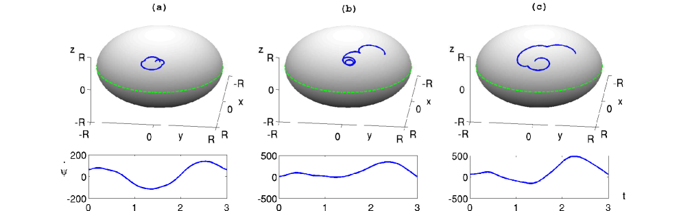
Figure 5: Optimal control results of the spinning disc on rotating earth. In the first row, we show trajectories in solid line and the equator in dotted line. In the second row, we present the spinning velocities correspondingly. End time is 3 days for all examples. Initial and final conditions are: (a) $(\phi_{0},\lambda_{0})=(\pi/4,0)$, $(\dot{\phi}_{0},\dot{\lambda}_{0},\dot{\psi}_{0})=(0,0,10\Omega)$, $(\phi_{f},\lambda_{f})=(\pi/4,0.1)$, $(\dot{\phi}_{f},\dot{\lambda}_{f},\dot{\psi}_{f})=(0,0,10\Omega)$; (b) $(\phi_{0},\lambda_{0})=(\pi/4,0)$, $(\dot{\phi}_{0},\dot{\lambda}_{0},\dot{\psi}_{0})=(0,0,\Omega)$, $(\phi_{f},\lambda_{f})=(\pi/4,\pi/3)$, $(\dot{\phi}_{f},\dot{\lambda}_{f},\dot{\psi}_{f})=(0,0,\Omega)$; (c) $(\phi_{0},\lambda_{0})=(\pi/4,0)$, $(\dot{\phi}_{0},\dot{\lambda}_{0},\dot{\psi}_{0})=(0,0,10\Omega)$, $(\phi_{f},\lambda_{f})=(\pi/4,\pi/3)$, $(\dot{\phi}_{f},\dot{\lambda}_{f},\dot{\psi}_{f})=(0,0,10\Omega)$.

4.2 Implementation of the Optimization Problem

We employ the mid-point approximation to obtain the discrete quantities in Section 3. The cost function is a measure of total control effort, defined by

$$J=\int_{t_{0}}^{t_{f}}(f_{\phi}^{2}+f_{\lambda}^{2}){\rm d}t,\quad J=\int_{t_{0}}^{t_{f}}f_{\psi}^{2}{\rm d}t,$$ (25)

for the particle and the spinning disc, respectively. The left and right discrete forces are approximated by $f^{-}_{n}=f^{+}_{n}=\frac{4}{h}(f_{n}+f_{n+1})$ and the discrete Lagrangian is given by

$$L_{d}(q_{n},q_{n+1})=hL\left(\frac{q_{n}+q_{n+1}}{2},\frac{q_{n+1}-q_{n}}{h}\right).$$ (26)

The discrete cost function for the particle is of the form

$$J_{d}=\sum^{N-1}_{n=0}\frac{h}{4}\left[(f_{\phi,n}+f_{\phi,n+1})^{2}+(f_{\lambda,n}+f_{\lambda,n+1})^{2}\right],$$ (27)

while that for spinning disc is

$$J_{d}=\sum^{N-1}_{n=0}\frac{h}{4}(f_{\psi,n}+f_{\psi,n+1})^{2}.$$ (28)

The solution procedure is as follow: (i) guess the trajectory for a small number of discrete steps, often the geodesic connecting starting and ending positions; (ii) solve the discrete optimization problem using sequential quadratic programming (SQP) method to obtain optimized trajectory and cost, done in Matlab; (iii) use result in (ii) as a reference in generating initial condition for more discrete steps, repeat (ii); (iv) compare the results, if the difference is small enough, numerical solution is obtained, otherwise repeat (iii).

4.3 Numerical Results of Motion Planning

The results for particle motion under optimal control are shown in Figure 4. Initial and final velocities are set to be zero for these simulations. Clearly, the optimal trajectories depend not only on the initial and final conditions but also on the time period $t_{f}-t_{0}$. In Figures 4(a) and 4(c), the time period is 1 day while the trajectories in 4(b) and 4(d) correspond to the same initial and final conditions but with a time period equal to 3 days. In order to arrive at final positions on time for 4(b) and 4(d), the particle must travel further, while for 4(a) and 4(c) the trajectories are obviously shorter. Yet the shorter trajectories come with the price of larger control efforts, $J_{d}|_{a}=66.2$, $J_{d}|_{b}=23.4$, $J_{d}|_{c}=54.7$ and $J_{d}|_{d}=14.3,$ which can be interpreted physically as follows: although the particle in 4(b) and 4(d) cover more distance, the fact that it has more time to reach its final destination means that it can better exploit the rotation of the earth.

The examples for a spinning disc under optimal control are shown in Figure 5. The first row illustrates the trajectories while the second row shows the corresponding spinning velocities $\dot{\psi}$. The initial and final conditions are: $\phi_{0}=\phi_{f}=\pi/4$, $\lambda_{0}=0$, and $\lambda_{f}$ are chosen to be $0.1$, $\pi/3$ and $\pi/3$ respectively, also $\dot{\phi}_{0}=\dot{\lambda}_{0}=\dot{\phi}_{f}=\dot{\lambda}_{f}=0$, and $\dot{\psi}_{0}=\dot{\psi}_{f}$ are chosen to be $10\Omega$, $\Omega$ and $10\Omega$ respectively. Since the control torque is only applied in $\psi$ direction, the disc is under-actuated and motion planning is harder than in the particle case. Comparing 5(a) with 5(c), one can observe that the trajectories have very similar behavior in the first half period. However, in the second half period, in order to travel further in 5(c), $\dot{\psi}$ needs to be increased more than that in 5(a), i.e. the control effort needs to be larger. Meanwhile, trajectories in 5(b) and 5(c) have similar behavior in the second half period, yet in the first half, the trajectories are quite different because of the different initial conditions. It is important to note that these examples result in net latitudinal changes. A net longitudinal motion seems not to be achievable by applying a control torque in $\psi$ only. This issue will be investigated in future work.

5 Summary

The motion planning for a particle and a spinning disc on earth was considered using an optimal control approach. These models are relevant for understanding geophysical vortex motion as well as for controlling the motion of atmospheric drifters such as high altitude balloons. In this paper, we employed an existing model of earth as a perfect sphere with an additional potential, then derived the equations governing the motion of a particle and a spinning disc moving on earth using Lagrangian mechanics, and showed solutions using direct numerical integration. We also examined the steady drift obtained in [6], and gave conditions for its validity. Motion planning for the particle and spinning disc was examined using discrete mechanics and optimal control. Rigorous proof of controllability of the spinning disc via one control torque about its spin axis remains an open question to be addressed in future work. Future directions include application of the earth model and the control methods used in this paper to the problem of multiple vortices on a sphere discussed in [8].

References

- [1] Cushman-Roisin, B. [1982], Motion Of A Free Particle On A Beta-Plane, Geophys, Astrophys, Fluid Dynamics, 22,85-102.
- [2] Durran, D.R. [1993], Is the Coriolis Force Really Responsible for the Inertial Oscillation?, Bull. Amer. Meteor. Soc., 74, 2179-2184
- [3] Grzybowski, B.A., H.A. Stone, G.M. Whitesides [2000], Dynamic Self-assembly of Magnetized, Millimeter-sized Objects Rotating at a Liquid-air Interface, Nature 405 pp 1033–1036.
- [4] Junge, O., Marsden, J.E. and Ober-Blobaum, S. [2005], Discrete Mechanics And Optimal Control, Proc. 16 IFAC Congr..
- [5] Kanso, E., Marsden, J.E. [2005], Optimal motion of an articulated body in a perfect fluid, Proc. CDC, 44, 2511-2516.
- [6] McDonald, N.R. [1998], The Time-Dependent Behaviour Of A Spinning Disc On A Rotating Planet: A model For Geophysical Vortex Motion, Geophys, Astrophys, Fluid Dynamics, 87, 253-272.
- [7] McIntyre, D.H. [2000], Using Great Circles To Understand Motion On A Rotating Sphere, Am. J. Phys., 68(12).
- [8] Newton, P.K. [2001], The -Vortex Problem: Analytical Techniques, Applied Mathematical Sciences, Vol. 145, Springer-Verlag.
- [9] Nijmeijer, H., Schaft, A.J.van der [1990], Nonlinear Dynamical Control Systems, Springer-Verlag
- [10] Paldor, N., Killworth, P.D. [1988], Inertial Trajectories On A Rotating Earth, J. Atmos. Sci., 45, 4013-4019.
- [11] Paldor, N., Sigalov, A. [2001], The Mechanics Of Inertial Motion On The Earth And On A Rotating Sphere, Physica D, 160, 29-53.
- [12] Paldor, N. [2005], Inertial Particle Dynamics On The Rotating Earth, earth.huji.ac.il
- [13] Ripa, P. [1997], ”Inertial” Oscillations and the -plane approximation(s), J. Phys. Oceanogr., 27, 633-647.
- [14] Ripa, P. [2000], Effects of the Earth’s Curvature on the Dynamics of Isolated Objects. Part I: The Disk, J. Phys. Oceanogr., 30, 2072-2087.
- [15] Ripa, P. [2000], Effects of the Earth’s Curvature on the Dynamics of Isolated Objects. Part II: The Uniformly Translating Vortex, J. Phys. Oceanogr., 30, 2504-2514.